Stanza: Layer Separation for Distributed Training in Deep Learning

Abstract

The parameter server architecture is prevalently used for distributed deep learning. Each worker machine in a such system trains the complete model, which leads to a large amount of network data transfer between workers and servers. We empirically observe that the data transfer has a major impact on training time.

We present a new distributed training system called Stanza to tackle this problem. Stanza exploits the fact that in many models such as convolution neural networks, most data exchange is attributed to the fully connected layers, while most computation is carried out in convolutional layers. Thus, we propose layer separation in distributed training: most nodes of the cluster train only the convolutional layers, while the rest train the fully connected layers. Gradients and parameters of the fully connected layers no longer need to be exchanged across the entire cluster, thereby substantially reducing the data transfer volume. We implement Stanza on PyTorch and evaluate its performance on Azure and EC2. Results show that Stanza accelerates training significantly over current parameter server systems: on EC2 instances with Tesla V100 GPU and 10Gb bandwidth for example, Stanza is 1.34x–13.9x faster for common deep learning models.

1 Introduction

Deep learning (DL) has recently achieved prominent success in many problem domains, particularly image classification [25, 39, 43, 18] and speech recognition [42]. As DL models are made more complicated and data are procured from more sources at a faster pace, distributed training becomes increasingly common in large organizations. Most distributed DL systems follow the parameter server architecture first proposed in [40] and later refined in [27, 19, 50, 6]. A parameter server system has two types of machines: workers and servers. Workers perform training on local data shards they are assigned to, and send the gradients of the model parameters to the corresponding servers. Servers update the parameters based on aggregated gradients from all workers, and push the latest parameters back to them for the next iteration.

In current parameter server systems workers train the complete DL model, and exchange the entire set of parameters with the servers in each iteration. This is termed the data parallelism paradigm. Given the sheer size of DL models with hundreds of millions of parameters [53, 25, 39, 43, 18], this approach produces an substantial amount of network data transfer. For example VGG-16 [39], Inception-V3 [43], and ResNet [18] have over 1100MB, 210MB, and 480MB data, respectively, that each worker has to exchange with servers in each iteration. Even with 40G or 100G interconnects the parameter exchange has a non-negligible impact on training time, especially when modern GPUs with tens of TFLOPs computation capacity are deployed [4].

Most DL models, in particular convolutional neural networks (CNNs), are composed of two basic building blocks: convolutional (CONV) layers and fully connected (FC) layers. More interestingly, we find that CONV and FC layers exhibit distinct characteristics (§ 3.1). CONV layers are essentially small filters that extract features through convolution over the training data. Thus they usually have a very small number of parameters ($<$10% of the total), but need a lot of computation ($>$90%). On the contrary, FC layers have full connectivity between layers in order to perform high-level reasoning. They generally use most of the parameters in the model, but only require a small amount of computation.

Motivated by these observations, we propose to decouple the training of CONV and FC layers instead of bundling them as in current parameter server architecture (§ 3.2). The idea is simple: We use most machines in the cluster as convolutional workers, or CONV workers, whose job is to train just the CONV layers that are computationally demanding. A few remaining machines then act as FC workers that train the FC layers and update their parameters. The FC layer gradient and parameter exchange, which accounts for most of the communication cost as discussed, now only happens among a few FC workers, which reduces the amount of data transfer and training time considerably.

To demonstrate the feasibility of our idea, we design and implement a new distributed DL system called Stanza (§ 4). Stanza’s design addresses two new challenges introduced by the separate training of models.

Communication Strategy. In order for training (with stochastic gradient descent [8, 23, 54]) to work, CONV workers now need to send activations of the last CONV layer to FC workers to complete the forward pass. Similarly FC workers need to push the gradients of the last CONV layer to CONV workers for backpropagation. Further, without centralized servers, CONV (resp. FC) workers need to exchange among themselves CONV (resp. FC) layer gradients.

Stanza adopts hybrid communication strategies to minimize the cost of these communication patterns (§ 4.1). For CONV-FC communication, since the number of activations of the last CONV layer is very small compared to the complete model, Stanza simply uses many-to-one and one-to-many communication here. For the more expensive gradient exchange among CONV (resp. FC) workers themselves, Stanza adopts efficient algorithms for the allreduce operation in the MPI literature [44] to fully parallelize the duplex communication among nodes. Stanza also overlaps the CONV worker and FC worker gradient exchange to further reduce the training time.

Node Assignment. The second design challenge is how to determine the node assignment in Stanza. That is, how many nodes in the cluster should be used as CONV/FC workers. We take a principled approach here (§ 4.2). First we develop a performance model to characterize Stanza’s training throughput for a given node assignment scheme based on the hybrid communication strategies. We then cast the node assignment problem as an optimization program that aims to maximize the training performance given the total number of nodes, which can be solved offline efficiently.

We implement Stanza on PyTorch [33] (§ 5) and evaluate it with small-scale deployments on Azure and AWS EC2 (§ 6). Our evaluation uses modern GPUs such as Nvidia Tesla V100 and widely used CNNs in image classification including AlexNet [25], VGG-16 and VGG-19 [39], Inception-V3 [43], and ResNet-152 [18]. We show that Stanza delivers significant speedup in training and saves up to 10x data transfer compared to parameter server systems. With 10 CONV workers and 1 FC worker for example, Stanza provides 13.9x and 8.2x speedups for AlexNet and VGG-16, respectively, using a 10G network. Even with 40G or 100G network bandwidth, our numerical simulation in § 7 shows that Stanza still provides salient benefits: it achieves 1.55x and 1.72x speedups for AlexNet and VGG-16, respectively, with 100G bandwidth.

2 Background

We start by introducing background on deep learning and the parameter server architecture.

2.1 Deep Learning

Deep learning (DL) is a class of machine learning algorithms that uses a large number of connected layers of different processing functions to handle complex tasks. The layered structure of DL models composes a large artificial neural network which resembles the biological structure of the human brain [26]. The objective of DL is to find a model that minimizes the difference between the inference result from the model and the ground truth, which is usually represented by a loss function. This is effectively an optimization problem and thus many optimization algorithms are used to iteratively train the DL models.

Particularly, stochastic gradient descent (SGD) is widely used in DL [8, 23, 41, 54]. The process consists of two phases with mini-batch SGD: forward pass and backpropagation. In the forward pass of the $t$-th iteration, a batch of input data $D_{t}$ is fed to the model, and a loss value $l(x,w_{t})$ is computed as the result for each sample $x$. Here $w_{t}$ represents model parameters. Then in backpropagation, the parameters are revised according to the loss so that the model “learns” about the correct answers. Mathematically, the parameter update rule is:

$$w_{t+1}\longleftarrow w_{t}-\frac{\eta}{n}\sum_{x\in D_{t}}\nabla l(x,w_{t}),$$ (1)

where $\eta$ is the learning rate and $n$ the batch size. The loss value is calculated at the output layer of the neural network, and gradients are generated from the output layer all the way back using the chain rule, so that parameters at each layer can be updated.

2.2 Parameter Server Systems

DL Training is usually done in a distributed setting with a cluster of machines in order to cope with the increasingly large datasets and complex models. The parameter server architecture has emerged as the de facto solution for distributed training since its inception [27, 50, 6], and is implemented in almost all DL frameworks [5, 10, 1].

Figure 1: The parameter server system. Each worker trains the complete model using its local data.

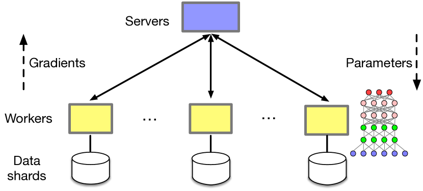
The parameter server (PS) system is a centralized design as shown in Figure 1. There are two types of nodes, servers and workers. A server node maintains a partition of the globally shared model parameters. Server nodes communicate with each other to replicate and/or to migrate parameters for reliability and scaling.A worker node performs training using data parallelism [54], and is responsible for one partition or shard of the training dataset. Each worker goes through a mini-batch (or simply batch) of its local data shard in parallel to compute gradients as discussed in § 2.1, and push them to the corresponding servers. Servers then aggregate the gradients from all workers to perform a global update of the model, and disseminate the new parameters to each worker. This completes one iteration of training. When workers go through all the samples in their shards in multiple iterations, they complete one epoch of training. Servers and workers are usually distinct machines for better fault-tolerance and performance.

2.3 Sizable Data Exchange in Training

Most DL models contain a large number of parameters in order to capture the complex features of the input data and their impact on the prediction results. Further, each worker needs to push the gradient of every parameter, and pull every updated parameter from the servers in each iteration. As a result, distributed training in a PS system entails a substantial amount of data exchange between workers and servers.

Table 1 shows the number of parameters for common DL models in image classification, and the corresponding data exchange volume per iteration in a PS system with 4 workers and 1 server. All workers send gradients to and receive parameters from the server. With tens or hundreds of millions of parameters, the PS server has to transfer about 0.8GB to 4.4GB data over the network. The bulky data transfer incurs non-negligible overhead to training time performance. The impact can be considerable especially as GPUs are now prevalently used to train large DL models. Owing to the high memory bandwidth and massive number of cores, GPU accelerates the matrix computation in DL tremendously, leaving the system more susceptible to other overheads such as the network data transfer.

Model	# Para.	Data Size (MB)	Measured	Estimated
			Training Time	Comm. Time
AlexNet [25]	61.1M	488.8 $\times$ 4	1.99s	1.56s
VGG-16 [39]	138M	1104 $\times$ 4	4.93s	3.53s
VGG-19 [39]	143M	1144 $\times$ 4	5.15s	3.66s
Inception-V3 [43]	27M	216 $\times$ 4	0.83s	0.69s
ResNet-152 [18]	60.2M	481.6 $\times$ 4	1.86s	1.54s

Table 1: Number of model parameters of popular DL models and its impact on training time per iteration with ImageNet-12 [35] and p3.2xlarge instances in AWS EC2. Each instance has a Nvidia Tesla V100 GPU and 10Gb bandwidth. Training time results are averaged over 100 iterations. Our PyTorch based PS implementation is used here with 1 server and 3 workers. Data size includes both gradients and parameters. Comm. time is estimated by dividing total data size over 10G. Other hyperparameters are explained in § 6.1.

To demonstrate the problem, we implement a PS system on PyTorch [33] and use an EC2 GPU cluster with the same setup above (4 workers and 1 server). We use p3.2xlarge instances each with a state-of-the-art Nvidia Tesla V100 datacenter GPU [4] and 10Gbps bandwidth, and train the DL models listed in Table 1. More details of the implementation and testbed setup can be found in the evaluation section § 6. We measure the per iteration training time by inserting timestamps before and after each iteration in the Python code. Note operations in PyTorch are executed immediately when the Python statements are invoked due to its dynamic graph design [33]; we do not add any extra barriers. The results averaged over 100 iterations are shown in Table 1. We also show the estimated communication time to complete the data transfer at the single server, which is calculated simply by dividing the data size by the 10G bandwidth.

Observe from Table 1 that the estimated communication time takes $\sim$70%–80% of the measured training time for all models. Note that actual impact of communication time may be less severe due to various optimization techniques such as overlapping communication with computation. Nonetheless, the results reflect that data transfer has a critical impact on distributed training with GPUs in PS systems. Prior work [53, 49, 38] has reported similar observations and the problem has attracted increasing attention recently in both DL [29, 47] and systems [53, 21] communities.

The impact of data transfer certainly can be mitigated with higher network bandwidth, which would require additional time and investment for the infrastructure overhaul. On the other hand the problem may also aggravate with the rapidly improving GPU or special-purpose hardware (ASIC, FPGA) that slashes computation time. We therefore ask, is the massive data transfer unavoidable in distributed training? Can we take a more fundamental approach to minimize the data transfer and the training time in turn without affecting the convergence or accuracy of the model?

Note that some ML frameworks such as MXNet [10] designate each node as both a worker and a server [49]. Each node is responsible for $1/N$ of the model parameters. This can mitigate the bandwidth bottleneck at the servers. However, the amount of parameters each node needs to send and receive is still massive ($4(N-1)/N$ parameters), which does not fundamentally overcome the issue. It is estimated that for such a system, the network bandwidth has to be at least 26Gbps in order for it not to become the bottleneck when training AlexNet on Titan X GPU [53], which is slower than the state-of-the-art GPUs now. Shi et al. [38] also report that MXNet has relatively high communication overhead when scaling to multiple nodes even with 56Gb Infiniband.

3 Separating the Layers

To answer our quest, we examine the characteristics of DL models, and propose to separately train the layers in order to substantially reduce the data transfer in distributed training. We focus on convolutional neural networks (CNNs) which are arguably the most widely used class of DL models.

3.1 Layers are Remarkably Different

(a) AlexNet

(b) VGG-16

Figure 2: Two common CNNs. AlexNet [25] has 5 CONV layers and 3 FC layers; VGG-16 [39] has 13 CONV layers and 3 FC layers. Other types of layers such as the pooling layer do not contain parameters; they just compute a fixed function of the inputs from the previous layer. Numbers of parameters are indicated in parentheses.

CNNs have been successfully applied in image recognition [25, 39, 43, 18], video analysis [50], natural language processing [22], drug discovery [14], etc. A CNN typically consists of two core building blocks, convolutional (CONV) layers and fully connected (FC) layers [25, 39, 43, 18]. A CONV layer has a set of learnable filters each of which is spatially small (e.g. 5$\times$5 along width and height). During the forward pass of training, each filter is convolved across the input data to extract certain features at some spatial position of the input. The neural network learns filters that activate when they detect certain features (e.g. pointy ears, curled tails), which are then passed on to the successive layers. Thus CONV layers are usually positioned right after the input layer. After CONV layers, the high-level reasoning is performed by the FC layers. Neurons in an FC layer have connections to all outputs in the previous layer. FC layers employ classifiers such as softmax to classify the output.

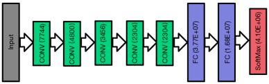
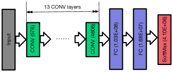
As a result of their functionality distinctions, CONV and FC layers exhibit remarkably different characteristics. CONV layers have a small number of parameters due to the small filters, but carry out a large amount of convolution computations. On the contrary, FC layers usually have a very large number of parameters due to its fully connected nature, but only require a small amount of simple calculations. As shown in Table 2 for example, for AlexNet and VGG-16, CONV layers incur most of the computations ($>$90%), while FC layers account for most of the parameters ($\sim$90%).

# FLOPs	CONV Layers	FC Layers
AlexNet	1.35E+09 / 92.0%	1.17E+08 / 8.0%
VGG-16	1.09E+10 / 98.9%	1.21E+08 / 1.1%

# Parameters	CONV Layers	FC Layers
AlexNet	2.47E+06 / 4.04%	5.86E+07 / 95.96%
VGG-16	1.47E+07 / 10.60%	1.24E+08 / 89.4%

Table 2: Estimated numbers of FLOPs and model parameters in AlexNet [25] and VGG-16 [39]. Data source: [52].

3.2 Separating CONV and FC Layers

The distinction between CONV and FC layers presents salient opportunities for us to optimize the communication cost of PS systems.

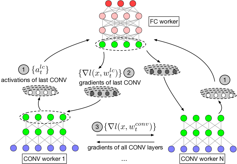
Specifically, it is now clear that much of the data transfer between workers and servers in a PS system is for FC layer parameters and gradients. Since CONV layers require most computation, we can assign most of the machines to train just the CONV layers, and the rest to train just the FC layers, as shown in Figure 3. With the separation of the layers, in the forward pass the CONV workers send the output of the last CONV layer, i.e. the activations, to the FC workers. The FC workers in turn send gradients of the last CONV layer back to CONV workers to continue backpropagation. FC layer gradients are now irrelevant to CONV workers, and no long need to be pushed over the network to each worker. As a result, a significant part of the communication in the traditional PS system can be eliminated to accelerate training. This is our key idea.

Figure 3: Training of CONV and FC layers are separated to reduce the data transfer, particularly for the FC gradients and parameters.

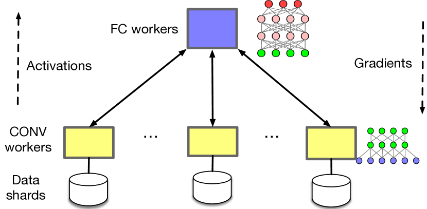
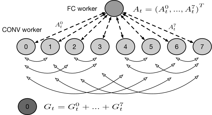
Training Process with Layer Separation. Figure 4 illustrates the training process with more detail. Suppose there is one FC worker now since most computation concentrates on CONV layers. In each iteration $t$, each CONV worker processes a sample up to the last CONV layer, and sends the activations from the last CONV layer to the FC worker. The FC worker collects all activations $a^{lc}_{t}$ for a batch of samples, and continues the forward pass to compute the loss values. It then starts backpropagation and computes gradients for all FC layers and the last CONV layer. It pushes gradients of the last CONV layer $\nabla l(x,w^{lc}_{t})$ to the CONV workers, and updates FC layer parameters. CONV workers then continue the backpropagation to compute their gradients in parallel, exchange them among all CONV workers to get global information $\sum_{x\in D_{t}}\nabla l(x,w^{conv}_{t})$ from all samples of the batch $D_{t}$, and perform CONV layer parameter update accordingly. This completes one iteration of training. The process is effectively equivalent to SGD in PS systems as explained in § 2.1.

Figure 4: The training process with the separation of CONV and FC layer training. At iteration $t$, CONV workers send activations of the last CONV layer $\{a^{lc}_{t}\}$ for a batch of samples to the FC worker. Then FC worker pushes gradients of the last CONV layer $\nabla l(x,w^{lc}_{t})$. Lastly CONV workers exchange gradients of all CONV layers to update parameters.

Note that a (max) pooling layer may follow the last CONV layer to reduce the number of activations. As discussed pooling layer does not have any parameters. Thus in this case we separate the model by the last pooling layer and include it in CONV workers to reduce communication between FC and CONV workers. This does not change the training process.

Benefits Overview. Now compared to PS, we eliminate the FC layer parameter exchange at the expense of: (1) sending activations and gradients of the last CONV layer, and (2) exchanging CONV layer gradients among CONV workers. First, comparing with the number of parameters of the entire model, the number of activations and gradients of the last CONV layer is small. For example, the number of activations from the last pooling layer in AlexNet is just 9216 for each sample [25]. With a typical batch size of 128, a CONV worker sends a total of $\sim$1.2M activations compared to 61.1M parameters for the entire model in each iteration. Second, the number of CONV layer parameters (gradients as well) is much smaller than that of large FC layers as discussed in § 3.1, and we can optimize the exchange with parallel communication to further reduce the time (§ 4.1). Thus, training time can be significantly improved by separating the CONV and FC layers.

Essentially, our idea of separating the training of CONV and FC layers, and using activations to replace gradients, can be regarded as a mixed use of both data parallelism and model parallelism in the DL literature [13]. Data parallelism—where each node trains the complete model with different data partitions—is prevalent in current DL systems due to implementation simplicity. We also employ data parallelism among CONV workers which train the same CONV layers independently with different data partitions. At the same time, training of FC layers is done on a separate group of workers which is an example of model parallelism. Amid the discussion about the two paradigms in the community [48, 13], our hybrid approach represents a promising alternative to the common conception of using one in lieu of the other exclusively.

4 Design

To demonstrate the feasibility of our idea, we design a new distributed DL system called Stanza. With the separate training of CONV and FC layers, Stanza needs to address two new challenges in system design: First, how to design the communication strategies between CONV and FC workers, and amongst CONV workers themselves in the backpropagation phase? Particularly, the CONV workers now need to synchronize parameters among themselves, and it is critical that Stanza minimizes such overhead. Second, how to assign the nodes to perform CONV or FC training, in order to ensure that the system performance is optimized in terms of training throughput?

4.1 Hybrid Communication

Stanza utilizes hybrid communication strategies to address the first design challenge we just presented. For simplicity, we start the discussion assuming only one FC worker in the system. We discuss the case of multiple FC workers in § 4.1.3. With one FC worker, communication in Stanza happens (1) between the CONV workers and the FC worker, and (2) among CONV workers themselves.

4.1.1 CONV-FC Communication

Activations of CONV workers are different since they process different input data. Thus gradients are also distinct for each CONV worker and has to be sent to the corresponding CONV worker in order for backpropagation to work. It is thus not possible to combine the activations or gradients to reduce the transmission volume. The number of activations and gradients of the last CONV layer is very small (a few MBs with a batch size of 128) and does not consume much bandwidth, as explained in § 3.2. Therefore, Stanza just uses simple many-to-one and one-to-many transmissions for CONV-FC communication as shown in Figure 5. This is also easy to implement.

Figure 5: Hybrid communication in Stanza. Dashed lines represent the many-to-one transmission from CONV workers to the FC worker, and one-to-many from FC worker to CONV workers. Solid lines represent the allreduce communication among CONV workers in backpropagation, which is orchestrated by the recursive doubling algorithm [44].

4.1.2 CONV Worker Communication

CONV worker communication is more demanding since most nodes in the cluster are CONV workers. The number of gradients of all CONV layers is also larger than activations: AlexNet for example has 2.3M CONV layer parameters compared to 1.2M activations with a batch size of 128. Moreover, performing the gradient exchange in an all-to-all manner generates a large volume of data transfer that scales quadratically with the number of workers, and is clearly not efficient. Note that the objective of CONV worker communication is to disseminate the global average gradients among all CONV workers, which is essentially an allreduce operation in MPI of parallel computing. Therefore we adopt an efficient implementation of allreduce called the recursive doubling algorithm [44] to schedule the communication. In recursive doubling, neighboring workers exchange data in the first round. Then workers that are two nodes away from each other exchange the reduced data from the first round. Generally workers exchange cumulative data with nodes $2i-1$ spots away in round $i$, as illustrated in Figure 5. In this case it requires $\log_{2}8$, i.e. 3 rounds to complete allreduce with 8 CONV workers.

If the number of CONV workers $n_{c}$ is not a power of two, we first randomly pick $n_{c}-2^{\lfloor\log_{2}n_{c}\rfloor}$ “surplus” nodes and have them send their gradients to another $n_{c}-2^{\lfloor\log_{2}n_{c}\rfloor}$ nodes randomly in parallel. Then recursive doubling can be applied on the $2^{\lfloor\log_{2}n_{c}\rfloor}$ nodes without the surplus ones. Finally the result is sent to surplus nodes in one round in parallel by $n_{c}-2^{\lfloor\log_{2}n_{c}\rfloor}$ random nodes. In other words it takes $\lfloor\log_{2}n_{c}\rfloor+2$ rounds to finish the allreduce.

4.1.3 FC Worker Communication

Finally in the case of multiple FC workers, each is responsible for an equal number of the CONV workers. Many-to-one and one-to-many communication strategies are then used between the corresponding FC and CONV workers. Each FC worker maintains a complete set of FC layers. Among the FC workers, Stanza relies on the same recursive doubling algorithm described above to exchange gradients and parameters efficiently. Further, FC worker communication is overlapped with CONV worker communication to reduce training time, since FC workers can start the parameter exchange after sending gradients to CONV workers.

4.2 Node Assignment

We now proceed to discuss how Stanza allocates the number of FC and CONV workers.

There are many tradeoffs involved in node assignment. For example, the number of CONV workers determines the total batch size: more CONV workers enables more images to be trained in parallel at each iteration. At the same time, more activations have to be sent to the FC workers who also need to send back more gradients as well, and the communication among CONV workers also takes longer to complete. Thus we rely on a principled approach to tackle this challenge: First we develop a performance model to characterize the key tradeoffs and their impact on Stanza’s training throughput, given a particular node assignment scheme. Then the optimal node assignment is obtained by solving the throughput maximization problem given the total number of nodes.

4.2.1 A Performance Model

We consider a homogeneous setting where each node has identical hardware resources. The key notations in our model are summarized in Table 3. Lower case notations denote unknowns and upper case notations are known constants. For tractability, our model only captures the ideal case performance without considering various overheads in for example node synchronization and parallelization, which are rather difficult to model explicitly.

$N$	total number of nodes
$n_{c},n_{f}$	number of CONV workers and FC workers
$K$	per-node batch size
$P$	total number of parameters in the DL model
$A$	number of activations of the last CONV layer
$P_{c}$	number of parameters in all CONV layers
$B$	bandwidth at each node
$t^{c}_{s}$	computation time per iteration Stanza
$T_{c}$	single worker CONV layer computation time per iteration
$T_{f}$	single worker FC layer computation time per iteration for one CONV worker’s activations
$t_{s}$	total training time per iteration for PS and Stanza

Table 3: Notation in the performance model.

We first characterize the computation time per iteration in Stanza $t^{c}_{s}$. There are two components: (1) CONV computation time $T_{c}$, including time to compute activations in the forward pass, and time to compute CONV layer gradients in backpropagation. This term only depends on the per-node batch size and a node’s GPU resources, and is constant with respect to node assignment since CONV workers work in parallel. (2) FC computation time, including the time to finish the forward pass based on activations, and then generate gradients for the FC layers. Denote the FC computation time to handle activations from one CONV worker on one FC worker as $T_{f}$. It is also constant since $T_{f}$ only depends on the per-node batch size and a node’s GPU resources. With $n_{c}$ CONV workers, the FC computation time grows to $n_{c}T_{f}$ due to the increase in activations, and with $n_{f}$ FC workers it becomes $\frac{n_{c}}{n_{f}}T_{f}$ due to parallel processing. Taken everything together, we have:

$$t^{c}_{s}=T_{c}+\frac{n_{c}}{n_{f}}T_{f}.$$ (2)

Now consider communication time in each iteration, which includes (1) CONV-FC communication time, (2) FC worker communication time, and (3) CONV worker communication time. Notice that (2) and (3) overlap in time as explained in § 4.1.3. Thus we do not consider FC worker communication here.

CONV workers send $n_{c}AK$ activations of the last CONV layer to the FC workers, which in turns send back $n_{c}AK$ gradients. Thus, CONV-FC communication takes ${2n_{c}AK}/{n_{f}B}$. CONV worker communications takes ${log_{2}n_{c}}$ rounds if $n_{c}$ is a power of 2, and $\lfloor log_{2}n_{c}\rfloor+2$ rounds if otherwise as explained in § 4.1.2. Each round takes $P_{c}/B$. Therefore, training time per iteration in Stanza, including communication and computation, can be written as:

$$t_{s}=\begin{cases}t_{s}^{c}+\frac{2n_{c}AK}{n_{f}B}+\frac{P_{c}log_{2}n_{c}}{B},&\text{if }n_{c}\text{ is a power of 2,}\\ t_{s}^{c}+\frac{2n_{c}AK}{n_{f}B}+\frac{P_{c}\left(\lfloor log_{2}n_{c}\rfloor+2\right)}{B},&\text{otherwise.}\end{cases}$$ (3)

The performance of a distributed DL system is characterized by training throughput, i.e. how many samples can be processed in unit time. We know that the total batch size is $n_{c}K$ in Stanza, i.e. with $n_{c}$ CONV workers it processes $n_{c}K$ samples in one iteration. Hence, its training throughput can be expressed as:

$$throughput_{s}(n_{c},n_{f})=\frac{n_{c}K}{t_{s}}.$$ (4)

4.2.2 Node Assignment

Observe from the performance model that a larger $n_{c}$ increases the total batch size, but also increases the computation time $t_{s}$ and communication time. Node assignment then strives to maximize the throughput of the cluster given the total number of nodes $N$. Mathematically, the optimal node assignment solves the following program:

$$\underset{n_{c},n_{f}}{\text{maximize}} throughput_{s}(n_{c},n_{f})$$ (5)

subject to $$N=n_{c}+n_{f},$$

$$n_{c}>0,n_{f}>0.$$

The optimization program can be solved offline by an exhaustive search over all possible values of $n_{c}$, as the total number of nodes is at most hundreds or thousands in practice and the computational cost is very small. More discussion on searching for the optimal deployment policy is in § 8. Note that for a given CNN model, the constants $T_{c}$ and $T_{f}$ depend on the node’s GPU resources and can be profiled offline fairly accurately.

5 Implementation

We implement Stanza based on the popular DL framework PyTorch [33] and its distributed communication package with TCP as the backend. Our prototype has two main components: a controller that maintains the model and cluster configuration, and a communication library that can be used in PyTorch programs to handle parameter communication for both PS and Stanza. The software architecture is similar to prior implementation of distributed DL training [53].

Method	Owner	Description
push	Worker in PS	Send gradients to the corresponding servers in PS
pull	Worker in PS	Receive updated parameters from the corresponding servers in PS
push_activation	CONV worker	Send activations of the last CONV layer to FC workers in Stanza
pull_fc	CONV worker	Receive gradients of the last CONV layer from the corresponding FC workers in Stanza
pull_grad	CONV/FC worker	Exchange gradients of all CONV/FC layers among CONV/FC workers in Stanza

Table 4: Communication APIs in our PyTorch prototype for both PS and Stanza.

5.1 Controller

The client program in PyTorch first instantiates our prototype by creating a controller within its process, and passing information about the entire CNN model and hyperparameters (e.g. batch size) to it. The program also specifies which architecture is to be used for distributed training, PS or Stanza.

For PS, the controller obtains the list of server and worker nodes, partitions the parameters equally across the servers by hashing, sends the mapping to each worker, and partitions the training data equally into data shards. It also sends the entire CNN model to workers to prepare for training.

For Stanza, the controller collects information about the throughput maximization program (5) in § 4.2.2 such as available bandwidth, single worker CONV/FC computation times ($T_{c}$ and $T_{f}$), etc., and solves the problem to compute the number of FC and CONV workers needed. It sends all FC layers and the last CONV layer to the FC workers, and all CONV layers to CONV workers. In case of multiple FC workers, the CONV workers are equally partitioned into $n_{f}$ groups and the mapping is maintained and synchronized by each CONV worker.

5.2 Communication Library

The communication library can be plugged into the training program. It provides APIs to support parameter communication with Stanza and PS as shown in Table 4. The push and pull methods are used by workers in PS to send gradients to servers, and acquire parameters from servers, respectively, based on the parameter mapping information. The pull method is called immediately after push, and blocks until it receives all parameter updates. The push method is nonblocking. The push and pull are implemented using PyTorch’s send and receive primitives, respectively, with the widely used bulk synchronous parallel (BSP) model [9].

For Stanza, the CONV workers invoke the push_activation method, which collects only activations from the last CONV layer for a batch of samples, then uses PyTorch’s send primitive to perform many-to-one communication to the corresponding FC workers. They then immediately call the blocking pull_fc method to obtain gradients of the last CONV layer from the corresponding FC workers. Finally, the pull_grad method is called by each CONV worker to perform gradient exchange with the recursive doubling algorithm discussed in § 4.1. It uses PyTorch’s all_reduce primitive. It blocks until the operation is finished for all CONV workers. It is also called by each FC worker to exchange gradients when there are more than one FC worker. The APIs for Stanza also apply BSP for model consistency.

5.3 Fault-Tolerance

For fault-tolerance, we use checkpointing throughout the system. Each node regularly creates checkpoints for current parameters and training state. In Stanza, there are very few FC workers. Thus a FC worker will create additional checkpoints for its FC parameters in a randomly chosen CONV worker. The redundant checkpoint is sent when both CONV and FC workers are training the model on GPUs, creating little overhead on training time.

6 Evaluation

We conduct testbed experiments on GPU clusters to assess the performance of the Stanza. We first verify its effectiveness with small datasets, by showing that Stanza achieves the same training accuracy as PS using 2x to 3.8x less time. Then we demonstrate the performance benefit of Stanza in production settings with large datasets and models, by showing that it achieves 1.34x to 13.9x speedup over PS, and the gain is more salient as the cluster grows.

6.1 Setup

Testbed in Public Clouds. To understand Stanza’s performance in a realistic environment, we deploy our PyTorch-based prototype on GPU clusters from two cloud providers, Azure and EC2. (1) We use standard_NC6 VMs from Azure as our first cluster. Each node is equipped with 6-core vCPUs, 56GB RAM, and a Nvidia Tesla K80 GPU (half of a physical card). Nodes are interconnected with high bandwidth, which we find to be $\sim$2.6Gbps. (2) For the EC2 cluster we use p3.2xlarge instances. Each node has 8-core vCPUs, 61GB RAM, and a Nvidia Tesla V100 GPU with 16GB RAM. The network bandwidth across nodes is 10Gbps. All nodes run Ubuntu 16.04, Nvidia driver version 384.13, CUDA 9.0, cuDNN 7.0, and PyTorch 0.3.1.

Stanza and PS always use the same number of nodes as CONV workers and workers, respectively, for fairness. Stanza uses 1 FC worker in all settings here. This does not imply that node assignment in § 4.2 is not useful. Instead, one FC worker is indeed optimal for throughput maximization when the cluster is smaller than 10 nodes in our testbeds. For larger clusters we need to use multiple FC workers as will be shown in § 7. PS also uses 1 server for fairness unless otherwise stated. Thus the total batch size is identical for the two systems, and we focus on training time per iteration as the performance metric here.

Datasets. We use two image classification datasets that are widely used in prior work [27, 53, 12, 5, 28]. (1) CIFAR-10 [24]: It is a small dataset consisting of 60K 32$\times$32 color images in 10 classes, with 50K training images and 10K validation images. (2) ImageNet-12 [35]: This is a large dataset used in the annual ImageNet Large Scale Visual Recognition Challenge (ILSVRC), with 1.28 million training images and 50K validation images in 1K classes.

Model	# Params	Dataset	Batch size
VGG-16 [39]	33.6M	CIFAR-10 [24]	128
AlexNet [25]	61.1M	ImageNet-12[35]	128
VGG-16 [39]	138M	ImageNet-12	64
VGG-19 [39]	143M	ImageNet-12	64
Inception-V3 [43]	27M	ImageNet-12	32
ResNet-152 [18]	60.2M	ImageNet-12	32

Table 5: Combinations of models and datasets used in the evaluation. Batch size is for each worker.

Models and Hyperparameters. We evaluate Stanza across many common CNNs for image classification. We list the model configurations in Table 5. We use the momentum SGD [15] as the optimization algorithm in both Stanza and PS. Small weight decay and dropouts are used to get better performance.

6.2 Baseline Performance

We first evaluate the baseline performance of Stanza using the small CIFAR-10 dataset and VGG-16. We modify the last softmax layer in the original VGG-16 in order to use CIFAR-10 with less classes, which reduces the number of parameters to 33.6M as shown in Table 5. Since the dataset and model are small, the experiments are done on the Azure cluster with less bandwidth. The same hyperparameters in Table 6 are used. Consistent with [39] we decrease the learning rate by 0.1 every 30 epochs. We train the model for 40 epochs. Recall that as in § 2.2, one epoch is one pass of the full training set and consists of many iterations during which each worker processes one batch of samples.

# (CONV)	Base	Total	System	Training	Accuracy
Workers	LR	batchsize		time (h)
2	0.2	256	Stanza	1.78	92.21%
			PS	3.64	90.95%
4	0.4	512	Stanza	1.22	91.52%
			PS	3.76	90.54%
8	0.8	1024	Stanza	0.93	89.80%
			PS	3.52	89.95%

Table 6: Baseline performance of Stanza with VGG-16 on CIFAR-10 using the Azure GPU cluster. We use 2, 4, and 8 CONV workers for Stanza and the same numbers of workers for PS, respectively. Per-node batchsize is 128. We use the same hyper-parameters and deployment policies for Stanza and PS in the same setting. We train for 40 epochs in each setting.

Table 6 shows the performance. Stanza effectively achieves the same (slightly better actually) accuracy of $\sim$90% compared to PS in all cases after 40 epochs. Further, Stanza brings significant savings in training time (at least 2x speedup), and the savings are more salient when the cluster grows. With 8 workers, Stanza obtains about 3.8x speedup compared to PS.

We also note that as the cluster grows the total training time for PS barely improves. The main reason is that network bandwidth is the bottleneck here, and though adding workers reduces the number of iterations per epoch, the amount of gradient and parameter transfer to/from the server also increases proportionally in PS. The total amount of gradient and parameter exchange per iteration stays the same as a result. We measure the time spent on computation in PS over 40 epochs, which is 0.47h and 0.25h for 4 and 8 workers, respectively. The numbers are reasonable, and they imply that the communication time is 3.29h and 3.27h with 4 and 8 workers, respectively.

Quick recap: The experiments here verify Stanza’s effectiveness: It improves training time by up to 3.8x compared to PS without trading off training accuracy, in settings with limited bandwidth.

(a) Speedup

(b) FC-Data

(c) Total-Data

Figure 6: Performance comparison with ImageNet-12 on large CNNs using the EC2 GPU cluster. PS uses one server and Stanza uses one FC worker for fairness. FC-Data and Total-Data are shown in log scale.

6.3 Performance for Large CNNs

We now use large CNNs to evaluate Stanza with the ImageNet-12 dataset. The experiments are done on the EC2 cluster with Tesla V100 GPUs and 10Gb bandwidth, which represent typical production settings for training DL models. One node is used as the server in PS and FC worker in Stanza, and up to 10 nodes are used as workers in PS and CONV workers in Stanza. The same hyperparameters in the previous section are used here, and the learning rate is linearly scaled with the cluster size. Training lasts for 30 epochs and both PS and Stanza achieve same accuracy, and we omit the accuracy results for brevity.

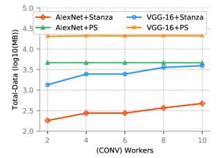
We focus on three performance metrics now: (1) Speedup: This is the ratio between training times of PS and Stanza. Larger speedup indicates better training time improvements. (2) FC-Layer Data Transfer (FC-Data): This is the amount of data transfer needed (in MB) to update the FC layer parameters in each iteration. Since we use 1 FC worker, FC-Data for Stanza effectively includes the number of activations and corresponding gradients only. (3) Total Data Transfer (Total-Data): Total-Data is defined as the total amount of data transfer (in MB) across all nodes in the system in an epoch. We use different time granularities for Total-Data and FC-Data to provide more insights into the performance analysis. Note that with the ImageNet-12 dataset an epoch has many iterations now. For example from Table 5, an epoch has 1251 iterations when we train AlexNet with 8 workers and a per-worker batch size of 128.

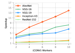
Figure 6 depicts the performance results with a varying number of (CONV) workers. We make two interesting observations here. First Stanza consistently shows salient speedups from 1.34x to 13.9x over PS as shown in Figure 6a. Among all models, AlexNet has the best speedup, and Inception-V3 and ResNet-152 the smallest. This is because Inception-V3 and ResNet-152 have proportionally more parameters in the CONV layers than other models, so the benefit of eliminating FC layer parameter exchange is not as substantial.

Second, the speedup in general increases as the cluster size grows. The main reason is that network is the bottleneck for PS even with 10Gb bandwidth, and adding workers to accelerate computation only slightly reduces the total training time. On the contrary, Stanza cuts the communication time significantly by replacing gradients with activations, and thus the benefit of parallelism from adding workers prevails.

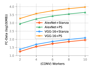
Figure 6b and 6c corroborate the above analysis. We only show the results for AlexNet and VGG-16 for brevity. Figure 6b shows that PS requires $\sim$100x larger data transfer than Stanza for FC layers, which is the main reason for Stanza’s training time improvement. FC-Data increases with more workers because in one iteration, the amount of FC layer data transfer depends on the total batch size and scales with the number of workers. Figure 6c shows the Total-Data comparison. Observe that PS’s total data transfer per epoch is over 4x larger than Stanza’s for all cluster sizes (the figure is in log-scale). In other words, PS needs to perform data transfer that is at least 4 times larger than Stanza. Total-Data of PS does not change with number of workers because although FC-Data per iteration increases with more workers, the number of iterations decreases proportionally. Essentially Total-Data in PS only depends on the total number of samples. Total-Data of Stanza increases slightly with more CONV workers because the CONV worker communication takes more rounds to complete based on the analysis in § 4.2.1.

Quick recap: We demonstrate that in production settings with 10G bandwidth and state-of-the-art data center GPU, Stanza provides significant improvements in training time over PS, which increases as the cluster size grows.

7 Numerical Results

Our evaluation so far covers small and medium clusters with typical GPU and bandwidth settings in public clouds. In reality, companies may use larger clusters for training with huge data. Also some clusters may deploy faster networks (40GbE, 100GbE, or RDMA) [2]. Yet it is difficult for us to access these hardware resources especially in a large scale.

Therefore in this section, we numerically evaluate Stanza in large-scale settings based on the empirical data from testbed experiments in § 6 and the performance model in § 4.2.1. We first develop a performance model for PS systems, similar to the one for Stanza, to estimate the training time and throughput. Then we verify the fidelity of the two models with experiments in public clouds. Finally, we estimate the throughput of both systems in large-scale settings using the performance models.

7.1 Performance Models and Verification

The performance model for Stanza is explained in detail in § 4.2.1. Here we develop a similar model for PS. Denote the computation time to process a batch of samples on one worker, including the forward pass and backpropagation, as $T_{ps}$. With $n_{s}$ servers, each is responsible for an equal share of ${P}/{n_{s}}$ parameters. The communication time in each iteration composes of (1) each server receiving ${P}/{n_{s}}$ gradients from each worker, which takes $n_{w}{P}/{n_{s}}B$ time, and then (2) each server sending ${P}/{n_{s}}$ parameters to each worker, which takes $n_{w}{P}/{n_{s}}B$ as well. Thus, training time per iteration is

$$t_{ps}=\frac{2n_{w}P}{n_{s}B}+T_{ps}.$$ (6)

Training throughput is then

$$throughput_{ps}(n_{w},n_{s})=\frac{n_{w}K}{t_{ps}}.$$ (7)

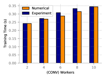
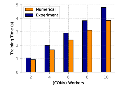
We measure $T_{ps}$ in PS and the single worker computation times $T_{c}$ and $T_{f}$ for Stanza in our EC2 GPU cluster, and feed them to the performance models to estimate the per-iteration training time. The model estimation is compared against the empirical data to verify their fidelity. We use AlexNet on ImageNet-12 with the same setup in § 6.1 here. Figure 7 shows the results with varying number of (CONV) workers. Observe that our models are fairly accurate. Comparing to experimental results, our model in (3) estimates the per-iteration training time of Stanza with $\sim$5% errors, and Equation (6) estimates PS training time with $\sim$20% errors. The errors may be attributed to an array of factors our models do not capture, such as fluctuating network bandwidth, memory copy time between CPU and GPU, etc. More importantly, they are acceptable for our purpose here because our model underestimates PS’s training time, and thus serves as a conservative lower bound for the speedup comparison against Stanza.

(a) Stanza

(b) Parameter Server

Figure 7: Accuracy of the performance models using AlexNet on ImageNet-12 in the EC2 cluster.

(a) AlexNet

(b) VGG-16

(c) VGG-19

Figure 8: Numerical results for different CNNs in large-scale clusters using the performance models. Stanza and PS use 5, 10, 20, 40, and 80 nodes in total. The y-axis shows throughput in $10^{3}$ samples per second. The x-axis is not in linear scale.

7.2 Numerical Simulation

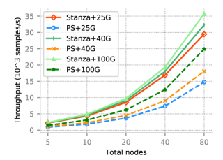
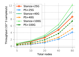
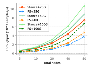
We now proceed to estimate the throughput performance of Stanza and PS in large-scale clusters. We use AlexNet, VGG-16, and VGG-19 on ImageNet-12, and obtain empirical data from our EC2 experiments for the model constants $T_{ps}$, $T_{c}$ and $T_{f}$. They reflect the computation performance on ImageNet-12 with Tesla V100 GPU, the fastest data center GPU presently. We assume each node has a single GPU. We vary the network bandwidth from 25G to 40G and 100G.

Stanza and PS use the same number of nodes in total, which varies from 5 to 80. Stanza applies the node assignment algorithm in § 4.2 to determine the optimal number of FC workers in each setting, which can be larger than one especially for large clusters. Similarly PS also uses the model in § 7.1 to obtain the throughput-maximizing node assignment in each case. For this reason the two systems may have different total batch sizes, and thus we focus on throughput instead of training time as the performance metric.

Figure 8 shows the numerical results. We make several observations. First, Stanza still outperforms PS significantly in a large cluster with fast network. With 80 nodes and 40G bandwidth for example, the throughput improvement is $\sim$1.79x for AlexNet, $\sim$1.97x for VGG-16, and $\sim$1.87x for VGG-19. Second, as the network bandwidth increases, communication becomes less of a problem, and Stanza’s improvement decays. At 25G bandwidth, training AlexNet, VGG-16, and VGG-19 can be improved by $\sim$2.29x, $\sim$2.35x, and $\sim$2.33x, respectively using Stanza with 40 nodes. When the bandwidth is 100G, Stanza’s benefit decreases to $\sim$1.55x, $\sim$1.72x, and $\sim$1.84x, respectively for the three CNNs.

Third, Stanza enjoys better scalability compared to PS. With 100G bandwidth, Stanza delivers 2x throughput improvement for AlexNet (resp. VGG-19) when the number of nodes increases from 40 to 80; PS only achieves 1.85x (resp. 1.73x) improvement in the same scenario. Lastly, a related observation is that PS’s scalability largely depends on the network bandwidth. Without enough bandwidth PS scales poorly due to again the communication bottleneck. For example with 25G bandwidth, PS has 1.73x, 1.81x, and 1.70x throughput benefits from 40 nodes to 80 for AlexNet, VGG-16, and VGG-19, respectively. With 100G bandwidth, the gains are better at 1.85x, 1.91x, and 1.73x, respectively. Stanza on the other hand consistently delivers 2x throughput scalability even with 25G bandwidth for all three CNNs.

Quick recap: Our numerical study shows that Stanza achieves $\sim$2x better throughput over PS in large-scale clusters with up to 100G bandwidth. Stanza also has better scalability due to its ability to remove the communication bottleneck.

8 Discussion

We discuss several concerns one may have about Stanza.

Beyond Parameter Server. Recently, to cope with the scalability issue of PS systems, new communication strategies for distributed training have been proposed and deployed in some cases. Uber proposes Horovod [37] which uses ring-reduce communication. Baidu’s internal system uses optimized allreduce communication [3]. This is orthogonal to our approach of reducing data transfer by layer separation, because both systems still rely on data parallelism with each node going through the complete model. For example we can use Horovod on the CONV workers to accelerate their communication. Stanza also applies to these non-PS systems to further improve training time, though we leave it as future work the implementation and evaluation of such an extension.

Beyond 10G Network Bandwidth. High bandwidth networks at 40G or 100G are deployed in some private data centers to speed up distributed training. However, 10Gbps network is the mainstream in public clouds and most private DL clusters. Clearly Stanza’s gain is less substantial with higher bandwidth since the impact of data transfer is smaller. Yet as we have numerically shown in § 7, Stanza still provides over 55% gain over the current PS systems with 100G bandwidth. As GPUs are improving at a rapid pace, we believe Stanza is instrumental for many deployment scenarios.

Beyond CNNs. We have focused on CNNs in this paper. The idea of layer separation works for many other DL models, where nodes exchange only the activations of the boundary layer instead of the full set of model parameters. For example, recurrent neural networks (RNNs) [17, 34] have recently received much attention with many applications [31, 16, 30]. Generally, an RNN model consists of cells each with the same multilayer perceptron (MLP) models, which have multiple FC layers without CONV layers. To show that our idea is also beneficial for RNNs, we consider the MLP in the RNN cells without dependency. We conduct a simple experiment, where an MLP is separated after the first 2 hidden layers, and we use just one node to train the last hidden layer and the output layer while the rest of nodes to train the first two hidden layers. As Table 7 shows, layer separation achieves 3.1x to 4.2x speedups over PS under the same resource and hyperparameter settings without sacrificing the accuracy. We plan to investigate in future work how to deal with the dependency between RNN cells in order to fully extend Stanza to RNN and other DL models.

Nodes	Base	Total	System	Training	Speedup	Accuracy
	LR	batchsize		time (s/epoch)
2	0.02	256	LS	16.8	3.1	53.37%
			PS	52.2		52.04%
4	0.04	512	LS	14.7	3.7	49.83%
			PS	54.6		48.97%
8	0.08	1024	LS	12.7	4.2	44.49%
			PS	53.0		45.79%

Table 7: Statistics for training MLP with layer separation (LS in the table) and PS. We use an MLP with 3 hidden layers each with 1024, 1024, and 4096 hidden units. We separate the model after the second hidden layer. We train the last hidden layer and the output layer with only one node, and the first two hidden layers with the rest of nodes. We use vanilla SGD to train the MLP for 100 epochs with learning rate decaying every 30 epochs. We use the Azure testbed as described in § 6.1 and CIFAR-10 as the dataset.

9 Related Work

We survey related work in this section.

Parameter Server Architecture. Parameter server has attracted much attention in both academia and industry since Distbelief [13]. Li et al. [27] propose a general PS system design that supports flexible model consistency, elastic scalability, and fault tolerance. Its variants and extensions have since been widely deployed. Examples include popular DL frameworks such as Tensorflow [5] and MXNet [10].

Several approaches have been proposed to deal with the communication problem in distributed training. We discuss some important ones other than those mentioned in § 8 now.

Communication Strategies. Xie et al. [49] propose sufficient factor broadcasting that transmits vectors to fully re-construct the parameter matrix. The amount of data transfer thus scales linearly instead of quadratically with the dimensions of the parameter matrix. Poseidon [53] exploits layered structures of DL models to overlap communication and computation and hide the communication cost. Both strategies can be applied in Stanza to further reduce the communication bottleneck.

Another approach is to use decentralized SGD algorithm [28] instead of centralized SGD. Nodes can be arranged in a ring topology. Each node only communicates with its neighbors instead of the entire cluster to exchange gradients and parameters at each iteration. This approach certainly speeds up the training time per iteration. Yet it demands multiple iterations to populate the parameters across the entire cluster, and the convergence speed may degrade in the end in practice.

Synchronization. Current PS systems generally use Bulk Synchronous Parallel (BSP) [45] to ensure model consistency among workers. BSP tends to prolong training time when stragglers are present. Asynchronous Parallel (ASP) and Stale Synchronous Parallel (SSP) [19, 46] alleviates the impact of stragglers by removing the barriers in BSP. Yet they deteriorate the convergence speed and model performance due to the staled parameter information [9]. How to achieve a good tradeoff between convergence and synchronization is still an open problem. Stanza adopts BSP in order to achieve fast convergence and better performance. It can also be readily extended to use ASP or SSP.

Gradient Compression. Another interesting approach is to compress the gradients and parameters. Gradient sparsification exploits the fact that the parameter matrix is sparse and some weights are small. Aji et al. [7] propose to truncate the insignificant gradients and only transmit the larger ones. Hsieh et al. [20] use a similar method that only sends important gradients to servers in a WAN setting. Gradient quantization reduces the number of bits to represent gradients and parameters [29]. CNTK [51] reduces the size of gradients via 1-bit quantization, which performs fairly well in speech recognition [36]. TernGrad [47] uses 2-bit quantization and is shown to have little accuracy loss. Stanza is orthogonal to these efforts, and can use them to further alleviate the communication cost.

10 Conclusion and Future Work

We have presented the design and implementation of Stanza, a communication-efficient DL system for distributed training. Stanza utilizes the unique characteristics of CNNs to separate the training of CONV and FC layers. FC layer parameter exchange is limited to among a few FC workers as a result, and the bulky data transfer across the network in conventional parameter server systems is largely removed. Testbed experiments in Azure and EC2 show that Stanza improves training time substantially over parameter server systems with latest datacenter GPUs and 10G bandwidth. Numerical studies also indicate that Stanza still provides modest speedup even with 100G bandwidth in large-scale clusters.

In this work we decouple the DL model at the boundary of CONV and FC layers, which is intuitive and easy to implement. As future work, other strategies of model decomposition [11] can be considered to further re-distribute computation. For example multiple decompositions can be realized by using additional machine groups to train the specific model partitions. The performance model may also be modified correspondingly for optimal node assignment. Other than layer based model decomposition, it is also possible to use more fine-grained model decomposition. For example it has been shown that scheduling the different operations of DL training to different computing devices can also improve training speed, though finding the optimal device placement itself is computationally expensive [32]. Extending Stanza to non-PS systems and general DL models is also a promising direction of future work as detailed in § 8.

References

- [1] Paddlepaddle. http://paddlepaddle.org.
- [2] Top-3 Ethernet Interconnect Considerations for your Machine Learning Infrastructure. http://www.mellanox.com/blog/2018/03/ethernet-interconnect-consi-derations-machine/-learning-infrastructure/.
- [3] Baidu-Research/Tensorflow-Allreduce. https://github.com/baidu-research/tensorflow-allreduce/, 2017.
- [4] Nvidia Tesla V100. https://www.nvidia.com/en-us/data-center/tesla-v100/, 2018.
- [5] M. Abadi, P. Barham, J. Chen, Z. Chen, A. Davis, J. Dean, M. Devin, S. Ghemawat, G. Irving, M. Isard, M. Kudlur, J. Levenberg, R. Monga, S. Moore, D. G. Murray, B. Steiner, P. Tucker, V. Vasudevan, P. Warden, M. Wicke, Y. Yu, and X. Zheng. TensorFlow: A System for Large-Scale Machine Learning. In Proc. OSDI, 2016.
- [6] A. Ahmed, M. Aly, J. Gonzalez, S. Narayanamurthy, and A. J. Smola. Scalable inference in latent variable models. In Proc. ACM WSDM, 2012.
- [7] A. F. Aji and K. Heafield. Sparse Communication for Distributed Gradient Descent. https://arxiv.org/abs/1704.05021, 2017.
- [8] L. Bottou. Large-scale machine learning with stochastic gradient descent. In Proc. COMPSTAT. 2010.
- [9] J. Chen, X. Pan, R. Monga, S. Bengio, and R. Jozefowicz. Revisiting distributed synchronous SGD. 2016.
- [10] T. Chen, M. Li, Y. Li, M. Lin, N. Wang, M. Wang, T. Xiao, B. Xu, C. Zhang, and Z. Zhang. MXNet: A flexible and efficient machine learning library for heterogeneous distributed systems. https://arxiv.org/abs/1512.01274, 2015.
- [11] A. Coates, B. Huval, T. Wang, D. Wu, B. Catanzaro, and N. Andrew. Deep learning with COTS HPC systems. In Proc. ICML, 2013.
- [12] A. Coates, A. Ng, and H. Lee. An analysis of single-layer networks in unsupervised feature learning. In Proc.International Conference on Artificial Intelligence and Statistics, 2011.
- [13] J. Dean, G. Corrado, R. Monga, K. Chen, M. Devin, M. Mao, A. Senior, P. Tucker, K. Yang, Q. V. Le, et al. Large scale distributed deep networks. In Proc. NIPS, 2012.
- [14] E. Gawehn, J. A. Hiss, and G. Schneider. Deep learning in drug discovery. Molecular informatics, 35(1):3–14, 2016.
- [15] P. Goyal, P. Dollár, R. Girshick, P. Noordhuis, L. Wesolowski, A. Kyrola, A. Tulloch, Y. Jia, and K. He. Accurate, large minibatch SGD: training imagenet in 1 hour. https://arxiv.org/abs/1706.02677, 2017.
- [16] A. Graves and N. Jaitly. Towards end-to-end speech recognition with recurrent neural networks. In Proc. ACM ICML, 2014.
- [17] A. Hannun, C. Case, J. Casper, B. Catanzaro, G. Diamos, E. Elsen, R. Prenger, S. Satheesh, S. Sengupta, A. Coates, et al. Deep speech: Scaling up end-to-end speech recognition. https://arxiv.org/abs/1412.5567, 2014.
- [18] K. He, X. Zhang, S. Ren, and J. Sun. Identity mappings in deep residual networks. In Proc. ECCV, 2016.
- [19] Q. Ho, J. Cipar, H. Cui, S. Lee, J. K. Kim, P. B. Gibbons, G. A. Gibson, G. Ganger, and E. P. Xing. More effective distributed ml via a stale synchronous parallel parameter server. In Proc. NIPS, 2013.
- [20] K. Hsieh, A. Harlap, N. Vijaykumar, D. Konomis, G. R. Ganger, P. B. Gibbons, and O. Mutlu. Gaia: Geo-Distributed Machine Learning Approaching LAN Speeds. In Proc. NSDI, pages 629–647, 2017.
- [21] F. N. Iandola, M. W. Moskewicz, K. Ashraf, and K. Keutzer. Firecaffe: near-linear acceleration of deep neural network training on compute clusters. In Proceedings of the IEEE Conference on Computer Vision and Pattern Recognition, pages 2592–2600, 2016.
- [22] Y. Kim. Convolutional neural networks for sentence classification. https://arxiv.org/abs/1408.5882, 2014.
- [23] S. Klein, J. P. Pluim, M. Staring, and M. A. Viergever. Adaptive stochastic gradient descent optimisation for image registration. International journal of computer vision, 81(3):227, 2009.
- [24] A. Krizhevsky, V. Nair, and G. Hinton. The CIFAR-10 Dataset. http://www.cs.toronto.edu/kriz/cifar, 2014.
- [25] A. Krizhevsky, I. Sutskever, and G. E. Hinton. Imagenet classification with deep convolutional neural networks. In Proc. NIPS, 2012.
- [26] Y. LeCun, Y. Bengio, and G. Hinton. Deep Learning. Nature, 521(7553):436, 2015.
- [27] M. Li, D. G. Andersen, J. W. Park, A. J. Smola, A. Ahmed, V. Josifovski, J. Long, E. J. Shekita, and B.-Y. Su. Scaling Distributed Machine Learning with the Parameter Server. In Proc. ACM OSDI, 2014.
- [28] X. Lian, C. Zhang, H. Zhang, C.-J. Hsieh, W. Zhang, and J. Liu. Can Decentralized Algorithms Outperform Centralized Algorithms? A Case Study for Decentralized Parallel Stochastic Gradient Descent. In Proc. NIPS, 2017.
- [29] Y. Lin, S. Han, H. Mao, Y. Wang, and W. J. Dally. Deep Gradient Compression: Reducing the Communication Bandwidth for Distributed Training. In Proc. ICLR, 2018.
- [30] S. Liu, N. Yang, M. Li, and M. Zhou. A recursive recurrent neural network for statistical machine translation. In Proceedings of the 52nd Annual Meeting of the Association for Computational Linguistics (Volume 1: Long Papers), volume 1, pages 1491–1500, 2014.
- [31] T. Mikolov, M. Karafiát, L. Burget, J. Černockỳ, and S. Khudanpur. Recurrent neural network based language model. In Eleventh Annual Conference of the International Speech Communication Association, 2010.
- [32] A. Mirhoseini, H. Pham, Q. V. Le, B. Steiner, R. Larsen, Y. Zhou, N. Kumar, M. Norouzi, S. Bengio, and J. Dean. Device Placement Optimization with Reinforcement Learning. https://arxiv.org/abs/1706.04972, 2017.
- [33] A. Paszke, S. Gross, S. Chintala, and G. Chanan. PyTorch: Tensors and dynamic neural networks in Python with strong GPU acceleration, 2017.
- [34] O. Press and L. Wolf. Using the output embedding to improve language models. https://arxiv.org/abs/1608.05859, 2016.
- [35] O. Russakovsky, J. Deng, H. Su, J. Krause, S. Satheesh, S. Ma, Z. Huang, A. Karpathy, A. Khosla, M. Bernstein, A. C. Berg, and L. Fei-Fei. ImageNet Large Scale Visual Recognition Challenge. International Journal of Computer Vision (IJCV), 115(3):211–252, 2015.
- [36] F. Seide, H. Fu, J. Droppo, G. Li, and D. Yu. 1-bit stochastic gradient descent and its application to data-parallel distributed training of speech dnns. In Fifteenth Annual Conference of the International Speech Communication Association, 2014.
- [37] A. Sergeev and M. Del Balso. Horovod: fast and easy distributed deep learning in tensorflow. https://arxiv.org/abs/1802.05799, 2018.
- [38] S. Shi and X. Chu. Performance Modeling and Evaluation of Distributed Deep Learning Frameworks on GPUs. https://arxiv.org/abs/1711.05979, 2017.
- [39] K. Simonyan and A. Zisserman. Very deep convolutional networks for large-scale image recognition. In Proc. ICLR, 2015.
- [40] A. Smola and S. Narayanamurthy. An architecture for parallel topic models. Proc. VLDB, 2010.
- [41] I. Sutskever, J. Martens, G. Dahl, and G. Hinton. On the importance of initialization and momentum in deep learning. In Proc. ICML, 2013.
- [42] P. Swietojanski, A. Ghoshal, and S. Renals. Convolutional neural networks for distant speech recognition. IEEE Signal Processing Letters, 21(9):1120–1124, 2014.
- [43] C. Szegedy, V. Vanhoucke, S. Ioffe, J. Shlens, and Z. Wojna. Rethinking the inception architecture for computer vision. In Proc. IEEE CVPR, 2016.
- [44] R. Thakur, R. Rabenseifner, and W. Gropp. Optimization of collective communication operations in MPICH. The International Journal of High Performance Computing Applications, 19(1):49–66, 2005.
- [45] L. G. Valiant. A bridging model for parallel computation. Communications of the ACM, 33(8):103–111, 1990.
- [46] J. Wei, W. Dai, A. Qiao, Q. Ho, H. Cui, G. R. Ganger, P. B. Gibbons, G. A. Gibson, and E. P. Xing. Managed communication and consistency for fast data-parallel iterative analytics. In Proc. ACM SoCC, 2015.
- [47] W. Wen, C. Xu, F. Yan, C. Wu, Y. Wang, Y. Chen, and H. Li. TernGrad: Ternary Gradients to Reduce Communication in Distributed Deep Learning. In Proc. NIPS, 2017.
- [48] R. Wu, S. Yan, Y. Shan, Q. Dang, and G. Sun. Deep image: Scaling up image recognition. https://arxiv.org/abs/1501.02876, 2015.
- [49] P. Xie, J. K. Kim, Y. Zhou, Q. Ho, A. Kumar, Y. Yu, and E. Xing. Lighter-communication Distributed Machine Learning via Sufficient Factor Broadcasting. In Proc. UAI, 2016.
- [50] E. P. Xing, Q. Ho, W. Dai, J. K. Kim, J. Wei, S. Lee, X. Zheng, P. Xie, A. Kumar, and Y. Yu. Petuum: A new platform for distributed machine learning on big data. IEEE Transactions on Big Data, 1(2):49–67, 9 2015.
- [51] D. Yu and X. Huang. Microsoft computational network toolkit (cntk). 2015. A Tutorial Given at NIPS, 2015.
- [52] H. Zhang, Z. Hu, J. Wei, P. Xie, G. Kim, Q. Ho, and E. P. Xing. Poseidon: A System Architecture for Efficient GPU-based Deep Learning on Multiple Machines. https://arxiv.org/abs/1512.06216, 2015.
- [53] H. Zhang, Z. Zheng, S. Xu, W. Dai, Q. Ho, X. Liang, Z. Hu, J. Wei, P. Xie, and E. P. Xing. Poseidon: An Efficient Communication Architecture for Distributed Deep Learning on GPU Clusters. In Proc. USENIX ATC, 2017.
- [54] M. A. Zinkevich, M. Weimer, A. Smola, and L. Li. Parallelized stochastic gradient descent. In Proc. NIPS, 2010.