Asymptotic Distribution of Centralized $r$ When Sampling from Cauchy

Abstract

Assume that $X$ and $Y$ are independent random variables, each having a Cauchy distribution with a known median. Taking a random independent sample of size $n$ of each $X$ and $Y$, one can then compute their centralized empirical correlation coefficient $r$. Analytically investigating the sampling distribution of this $r$ appears possible only in the large $n$ limit; this is what we have done in this article, deriving several new and interesting results.

1 Introduction

It can be easily shown, based on Central Limit Theorem, that the sampling distribution of the usual sample correlation coefficient further multiplied by $\sqrt{n}$ i.e.

$$\frac{\sqrt{n}\cdot\sum_{i=1}^{n}\left(X_{i}Y_{i}-\frac{\sum_{i=1}^{n}X_{i}\cdot\sum_{i=1}^{n}Y_{i}}{n}\right)}{\sqrt{\sum_{i=1}^{n}X_{i}^{2}-\frac{\left(\sum_{i=1}^{n}X_{i}\right)^{2}}{n}}\sqrt{\sum_{i=1}^{n}Y_{i}^{2}-\frac{\left(\sum_{i=1}^{n}Y_{i}\right)^{2}}{n}}}$$

tends to, when $n\to\infty$ and $X_{i}$ and $Y_{i}$ are independent (both within and between), the standard Normal distribution whenever both $X$ and $Y$ have finite means and variances. The situation changes dramatically when sampling from a Cauchy distribution. Investigating what happens in that case is rather difficult; to simplify the task, we assume that the medians of $X$ and $Y$ are known, and can therefore be subtracted from the $X_{i}$ and $Y_{i}$ values. This amounts to assuming that the two Cauchy distributions have zero medians and it is then sufficient to define what we call the centralized sample correlation coefficient as

$$r_{c}=\frac{\sum_{i=1}^{n}X_{i}Y_{i}}{\sqrt{\sum_{i=1}^{n}X_{i}^{2}}\sqrt{\sum_{i=1}^{n}Y_{i}^{2}}}$$ (1)

It is obvious that the second parameter (the quartile deviation) of each of the two Cauchy distributions cancels out of the last expression; we can thus assume (without a loss of generality), that both the $X_{i}$ and $Y_{i}$ are drawn independently from a Cauchy distribution with median equal to 0 and the quartile deviation equal to 1. The objective of this article is to find the asymptotic (i.e. large-$n$) behaviour of $r_{c}$. This centralized $r_{c}$ is also known to others in the computer science, big data and data science fields as the cosine similarity measure. It has applications in text mining, data mining and information retrieval [1, 2]; an investigation of the statistical distribution related to this centralized $r_{c}$ has been done by [3].

2 Related Sampling Distributions

To obtain its asymptotic distribution, we must first explore the distribution of the individual terms of $r_{c}$. We start by quoting the probability density function (PDF) and the characteristic function (CF) of each $X_{i}$ and $Y_{i}$:

$$f\left(x\right)=\frac{1}{\pi\left(x^{2}+1\right)}$$

and

$$\varphi\left(t\right)=\exp{\left(-\left|t\right|\right)}$$

respectively (these are well-known results [4]).

This implies that the PDF each $X_{i}^{2}$ and $Y_{i}^{2}$ (denoted $Z$) is given by

$$f\left(z\right)=\begin{cases}\frac{\displaystyle 1}{\displaystyle\pi\sqrt{z}\left(z+1\right)}&z>0\\ 0&\textrm{elsewhere}\end{cases}$$ (2)

and the distribution function of $Z$ is given by

$$F_{X^{2}}\left(z\right)=\Pr\left(X^{2}\leq z\right)=\frac{1}{\pi}\int_{-\sqrt{z}}^{\sqrt{z}}\frac{\operatorname{d}\!{x}}{1+x^{2}}=\frac{2}{\pi}\arctan\sqrt{z}$$

The corresponding CF is then

$$\varphi_{X^{2}}\left(t\right)=\exp\left(-it\right)\left[1-\textrm{erf}{\left(\sqrt{-it}\right)}\right]$$ (3)

and can be found by taking the appropriate Fourier transform of the PDF [5]; here we rely on computer software (such as Maple or Mathematica) to provide these.

To obtain the asymptotic CF of each $\lim_{n\to\infty}\frac{\sum_{i=1}^{n}X_{i}^{2}}{n^{2}}$ and $\lim_{n\to\infty}\frac{\sum_{i=1}^{n}Y_{i}^{2}}{n^{2}}$ (denoted $W$), we have to raise $\eqref{eq:cf_cauchy_sq}$ to the power of $n$, replace $t$ by $\frac{t}{n^{2}}$ and then take the $n\to\infty$ limit of the resulting expression (note that only by dividing by $n^{2}$ can one reach a finite limit - that is how these ‘normalizing factors’ are found in general).

This yields

$$\varphi_{W}\!\left(t\right)=\exp\left(-2\sqrt{\frac{-it}{\pi}}\right)$$

since $\textrm{erf}{\left(x\right)}\simeq\frac{2x}{\sqrt{\pi}}$ for small $x$. The appropriate inverse Fourier transform converts this CF to the corresponding PDF, namely

$$f\!\left(w\right)=\begin{cases}\frac{\displaystyle\exp\left(-\frac{1}{\pi w}\right)}{\displaystyle\pi w^{\frac{3}{2}}}&w>0\\ 0&\textrm{elsewhere}\end{cases}$$ (4)

One can show via Monte Carlo simulation that this constitutes a fairly accurate approximation for the PDFs of $\frac{\sum_{i=1}^{n}X_{i}^{2}}{n^{2}}$ and $\frac{\sum_{i=1}^{n}Y_{i}^{2}}{n^{2}}$ even for relatively small $n$ values ($n\geq 30$). This is due to the fact that the corresponding CF can be expanded in increasing powers of $\frac{1}{n}$. The error of the approximation is thus of the $O\left(\frac{1}{n}\right)$ type which is faster than $O\left(\frac{1}{\sqrt{n}}\right)$ of the Central Limit Theorem.

The PDF of W can be readily converted into the (asymptotic) PDF of each $\lim_{n\to\infty}\frac{n}{\sqrt{\sum_{i=1}^{n}X_{i}^{2}}}$ and $\lim_{n\to\infty}\frac{n}{\sqrt{\sum_{i=1}^{n}Y_{i}^{2}}}$ (denoted $U$ and equal to $\frac{1}{\sqrt{W}}$) using a simple univariate transformation, yielding

$$f\!\left(u\right)=\begin{cases}\frac{\displaystyle\exp{\left(-\frac{u^{2}}{\displaystyle\pi}\right)}}{\displaystyle\pi}&u>0\\ 0&\textrm{elsewhere}\end{cases}$$ (5)

resulting in a half-normal distribution.

Finally, each of the $X_{i}Y_{i}$ (denoted $S$) has a CF found by

$$\int_{-\infty}^{\infty}\int_{-\infty}^{\infty}\exp(ixyt)\cdot\frac{1}{\pi\left(x^{2}+1\right)}\cdot\frac{1}{\pi\left(y^{2}+1\right)}\operatorname{d}\!{x}\operatorname{d}\!{y}$$

resulting in

$$\varphi_{S}\left(t\right)=\begin{cases}\frac{\displaystyle 2\left(\sin{\left|t\right|}\textrm{Ci}{\left|t\right|}-\cos{\left|t\right|}\textrm{Si}{\left|t\right|}\right)}{\displaystyle\pi}+\cos{\left|t\right|}&t\neq 0\\ 1&t=0\end{cases}$$

which corresponds to the relatively simple PDF

$$f\!\left(s\right)=\begin{cases}\frac{\displaystyle\ln\left(s^{2}\right)}{\displaystyle\pi^{2}\left(s^{2}-1\right)}&v=\mathbb{R}\setminus\left\{-1,0,1\right\}\\ \frac{\displaystyle 1}{\displaystyle\pi^{2}}&v=\left\{-1,1\right\}\\ 0&\textrm{elsewhere}\\ \end{cases}$$ (6)

Assuming that each $X_{i}Y_{i}$ (and also their sum) are asymptotically independent of $\frac{n}{\sqrt{\sum_{i=1}^{n}X_{i}^{2}}}$ and $\frac{n}{\sqrt{\sum_{i=1}^{n}Y_{i}^{2}}}$ (something we have been able to verify only empirically), we now find the CF of

$$X_{i}Y_{i}\cdot\frac{n}{\sqrt{\sum_{i=1}^{n}X_{i}^{2}}}\cdot\frac{n}{\sqrt{\sum_{i=1}^{n}Y_{i}^{2}}}\simeq S\cdot U_{1}\cdot U_{2}$$ (7)

where $U_{1}$ and $U_{2}$ are independent random variables, each having an asymptotic PDF of $\eqref{eq:pdf_denom_asymp}$. This resulting approximate CF is computed by

$$\frac{4}{\pi^{4}}\int_{0}^{\infty}\int_{0}^{\infty}\int_{-\infty}^{\infty}\cos\left(u_{1}u_{2}st\right)\cdot\exp\!\left(-\frac{u_{1}^{2}+u_{2}^{2}}{\pi}\right)\cdot\frac{\ln{s^{2}}}{s^{2}-1}\operatorname{d}\!{s}\operatorname{d}\!{u}_{1}\operatorname{d}\!{u}_{2}$$

where the usual $\exp(iu_{1}u_{2}st)$ has beeen replaced by $\cos(u_{1}u_{2}st)$, since the resulting distribution is symmetric, implying that it is CF has no imaginary part.

To simplify the $\operatorname{d}\!{u}_{1}\operatorname{d}\!{u}_{2}$ integration, we perform it in the usual polar coordinates (denoted $R$ and $\Theta$) getting

$$\frac{4}{\pi^{4}}\int_{0}^{\infty}int_{0}^{\frac{\pi}{2}}\int_{-\infty}^{\infty}R\cos\!\left(stR^{2}\frac{\sin{2\Theta}}{2}\right)\cdot\exp\left(-\frac{R^{2}}{\pi}\right)\cdot\frac{\ln{s^{2}}}{s^{2}-1}\operatorname{d}\!{s}\operatorname{d}\!{\Theta}\operatorname{d}\!{R}$$

$$=\frac{2}{\pi^{3}}\int_{0}^{\frac{\pi}{2}}\int_{-\infty}^{\infty}\frac{1}{1+\left(\pi st\frac{\sin{2\Theta}}{2}\right)^{2}}\cdot\frac{\ln{s^{2}}}{s^{2}-1}\operatorname{d}\!{s}\operatorname{d}\!{\Theta}$$

$$=\frac{2}{\pi}\int_{0}^{\frac{\pi}{2}}\frac{1+\left|t\right|\sin{2\Theta}\ln{\left(\pi\left|t\right|\frac{\sin 2\Theta}{2}\right)}}{1+\left(\pi t\frac{\sin{2\Theta}}{2}\right)^{2}}\operatorname{d}\!{\Theta}$$ (8)

3 Asymptotic PDF of $r_{c}$

To get an approximate CF of

$$\frac{\sum_{i=1}^{n}X_{i}Y_{i}}{n\ln n}\cdot\frac{n}{\sqrt{\sum_{i=1}^{n}X_{i}^{2}}}\cdot\frac{n}{\sqrt{\sum_{i=1}^{n}Y_{i}^{2}}}.$$ (9)

Note the unusual normalizing factor – the only way to achieve a finite limit. We need to first raise $\eqref{eq:cf_rc_term}$ to the power of $n$ while simultaneously replacing $t$ by $\frac{t}{n\ln{n}}$, taking the $n\to\infty$ limit and finally evaluating the remaining integral. These operations can be carried out in any order in this particular case - something not true in general.

This yields before the $\operatorname{d}\!{\Theta}$ integration

$$\exp\left(-\left|t\right|\sin{2\Theta}\right)+\mathcal{O}\!\left(\frac{1}{\ln{n}}\right)$$ (10)

Since the error of this approximation is proportional to $\frac{1}{\ln{n}}$, the actual convergence of the subsequent result is expected to be rather slow (reaching a good accuracy only when $n$ is at least a few hundred). One can recover a part of this error (trying to recover the full $\frac{1}{\ln{n}}$ proportional term would make the resulting expression too cumbersome) by replacing $\eqref{eq:cf_rc_asymp}$ with the more accurate

$$\exp\left(-a\left|t\right|\sin{2\Theta}\right)$$

where

$$a=1-\frac{\ln{\pi}}{\ln{n}}.$$

To complete the computation, we evaluate

$$\varphi_{r_{c}}\left(t\right)=\frac{2}{\pi}\int_{0}^{\frac{\pi}{2}}\exp{\left(-a\left|t\right|\sin{2\Theta}\right)}\operatorname{d}\!{\Theta}=I_{0}{\left(a\left|t\right|\right)}-L_{0}{\left(a\left|t\right|\right)}$$

where $I_{0}$ and $L_{0}$ are the Bessel and modified Struve functions respectively. Converting to PDF results in:

$$f\!\left(r_{c}\right)=\frac{2\ln\left(a+\sqrt{a^{2}+r_{c}^{2}}\right)-\ln r_{c}^{2}}{\pi^{2}\sqrt{a^{2}+r_{c}^{2}}}$$ (11)

which is our final answer for the approximate distribution of the sum of $\eqref{eq:rv_rc_sum}$ terms, which is the same as

$$\frac{n\cdot r_{c}}{\ln{n}}.$$ (12)

Note that similarly to the Cauchy distribution itself $\eqref{eq:pdf_rc_aymp}$ has an indefinite mean and an infinite variance.

4 Monte Carlo Verification

We will now verify the accuracy of our approximation by randomly generating $100,000$ values of $\eqref{eq:rv_rc_normalized}$, using $n=400$. The following Mathematica program does this and plots the corresponding histogram together with our approximate PDF $\eqref{eq:pdf_rc_aymp}$.

G[x_, y_] := x.y/Sqrt[x.y y.y]
n = 400;
superN = 100 000;
data = {};
Do[SeedRandom[];
  dataX = RandomReal[CauchyDistribution[], n];
  dataY = RandomReal[CauchyDistribution[], n];
  AppendTo[data, (n/Log[n]) * Apply[G, {dataX, dataY}]], {superN} ]

a = 1 - Log[Pi]/Log[n];
pdf = (2*Log[a + Sqrt[a^2 + x^2]] - Log[x^2]) / (Pi^2*Sqrt[a^2 + x^2]);
Show[Histogram[data, {-4, 4, 0.25}],
  Plot[0.25*superN*pdf, {x,-4,-4}, PlotRange -> {0,0.2*superN}]]

The two results are in good agreement, as can be seen in the Figure 1.

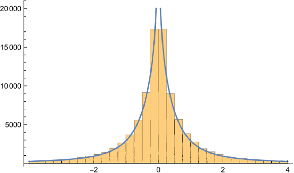
Figure 1: Histogram vs. Approximate PDF.

5 Conclusion

We have derived an asymptotic distribution of the centralized sample correlation coefficient when sampling from Cauchy distribution, discovering some of its unusual properties. As a byproduct, several other interesting distributions have been introduced in the process.

References

• [1] Tan, P-N, Steinbach, M, Kumar, Vipin: Introduction to Data Mining. Pearson Addison Wesley, Boston (2005)
• [2] Singhal, A: Modern Information Retrieval: A Brief Overview. Bul. IEEE on Data Engineering Vol 24. No 4. 35-43 (2001)
• [3] Giller, L. G: The Statistical Properties of Random Bitstreams and the Sampling Distribution of Cosine Similarity. (2012) doi:10.2139/ssrn.2167044
• [4] Johnson, N. L, Kotz, S, Balakrishnan, N: Continuous Univariate Distributions, Volume 1, Second Edition. Wiley, New York (1994)
• [5] Billingsley, P: Probability and Measure, 3rd Edition. John Wiley & Sons, New York (1995)