On the Beta Transformation

Abstract

The beta transformation is the iterated map $\beta x\,\mod 1$; it generates the base-$\beta$ expansion of a real number $x$. Every iterated piece-wise monotonic map is topologically conjugate to the beta transformation. For all but a countable subset of $\beta$, the orbits of $x$ are ergodic; yet it is the finite orbits that determine overall behavior.

This is a large text; it splits into four parts. The first part provides a review of general concepts and properties associated with the beta shift. The second part examines the spectrum of the Ruelle–Frobenius–Perron operator, and gives explicit expressions for a set of bounded eigenfunctions. These form a discrete spectrum, accumulating on a circle of radius $1/\beta$ in the complex plane.

The third part examines the finite and the periodic orbits. These are in one-to-one correspondence with monic integer polynomials. They are “quasi-cyclotomic” and can be counted with Moreau’s necklace-counting function; curiously, they do not have any obvious relation to other systems countable by the necklace function. The positive real roots are dense in the reals; they include the Golden and silver ratios, the Pisot numbers, the n-bonacci (tribonacci, tetranacci, etc.) numbers. The beta-polynomials yoke all of these together into a regular structure. An explicit bijection to the rationals is presented.

The fourth part of this text examines small perturbations. These introduce Arnold tongues, which inflate the finite orbits, a set of measure zero, to finite size.

This text assumes very little mathematical sophistication on the part of the reader, and should be approachable for any enthusiast with minimal or no prior experience in ergodic theory. Most of the development is casual. As a side effect, the introductory sections are perhaps a fair bit longer than strictly needed to present the new results.

linasvepstas@gmail.com

1 Introduction

Given a real number $x$, it can be written down in base-ten, decimal notation, as a string of digits 0-9. Each successive digit is given by an iterated formula. Starting with $y_{0}=x$, let

$$y_{n+1}=\left(10y_{n}\right)\mod 1$$

The $n$’th digit in the decimal expansion is $d_{n}=\left\lfloor y_{n}\right\rfloor$. Here, mod is the modulo (or remainder) function, so that $a\mod b$ is the remainder of $a$ after dividing by $b$. The bracket $\left\lfloor z\right\rfloor$ is the floor function, returning the largest integer less than $z$. The decimal expansion of $x$ is then $d_{0}.d_{1}d_{2}d_{3}\cdots$ with all digits $d_{n}$ (except for the first) running between 0 and 9. The iteration has the form of a shift; it shifts over by one digit, and repeats the process. The shift is ergodic over the reals: any and every decimal expansion will occur.

The same idea can be applied by replacing ten by any number $\beta$; this gives the base-$\beta$ expansion. The $\beta$ does not need to be an integer; the rest of this text is focused on exploring the expansions coming from $1<\beta\leq 2$, so “base two or less”.

The beta transformation is the map

$$t_{\beta}\left(x\right)=\beta x\mod 1$$

iterated on the unit interval $\left[0,1\right]$ of the reals, and $\beta$ taken to be a real positive constant. For the special case of $\beta=2$, this is the Bernoulli process, the ergodic process of random coin flips. The Bernoulli shift is solvable in more ways than one; it is well-understood, and provides a canonical model of ergodic behavior. The beta transformation is less well-known and less carefully scrutinized. A full review of previous results is presented at the end of this introduction. The goal of this text is two-fold: to expand the collection of known properties, and to present them in the simplest, most accessible fashion possible.

One primary driver of interest in iterated functions is that they generate fractals, and that they provide simple models of chaotic dynamics. The $\beta$-transform is the simplest possible map that exhibits all of the hallmarks of chaotic dynamical systems: a non-trivial, nonuniform invariant measure, with both periodic and non-periodic orbits. It is also “generic”, in that any other piecewise-monotonic map of the unit interval is topologically conjugate to it. If one can understand the $\beta$-transform, one has gone a long ways towards understanding iterated maps in general.

There are two broad approaches for studying iterated functions. One is to examine the point dynamics and orbits: “where does the point $x$ go, when iterated?”. The other is in terms of distributions: “how does a scattered dust of points evolve over time?”. Within the context of physics, these give two broad philosophical views of reality. The first is of microscopic, time-reversible systems whose future is deterministic and known with infinite precision. The second is of macroscopic, time-irreversible thermodynamics, where time can only go forward, and the future is unknown and unknowable. Of these two approaches, the first is commonplace and inescapable; the second remains obscure, poorly-recognized and opaque. Thus, a large part of this text is devoted to this second approach.

If iterating a map $x\mapsto f\left(x\right)\mapsto f\left(f\left(x\right)\right)\mapsto\cdots$ pulls a point $x$ through $f$, through time, then the action of the map $f$ on a distribution $\rho$ is a pushforward:

$$\rho\left(A\right)\mapsto\rho\left(f^{-1}\left(A\right)\right)\mapsto\rho\left(f^{-1}\left(f^{-1}\left(A\right)\right)\right)\mapsto\cdots$$

The proper definition of a pushforward requires a significant development of the concepts of measurable spaces and Borel sigma algebras, topics that will be gently reviewed a bit further in this introductory section. For the present, it is enough to take $\rho:\left[0,1\right]\to\mathbb{R}$ to be some function defined on the unit interval. In the above, $A\subset\left[0,1\right]$ is a subset of the unit interval, so that $\rho\left(A\right)=\int_{A}\rho\left(x\right)dx$ is an ordinary integral, the “size” of the set $A$ with respect to the distribution.

The challenge is to find an explicit expression for the pushforward $\rho\left(f^{-1}\left(A\right)\right)$. This can be obtained as a change of variable $y=f\left(x\right)$ under integration. Start with any function $h$; it’s integral over the set $A$ is as above: $h\left(A\right)=\int_{A}h\left(y\right)dy$. Under the change of variable, this becomes

$$h\left(A\right)=\int_{A}h\left(y\right)dy=\int_{f^{-1}\left(A\right)}h\left(f\left(x\right)\right)\left|f^{\prime}\left(x\right)\right|dx$$

Writing the integrand as $\rho\left(x\right)=h\left(f\left(x\right)\right)\left|f^{\prime}\left(x\right)\right|$ and working backwards, one recovers

$$h\left(y\right)=\frac{\rho\left(f^{-1}\left(y\right)\right)}{\left|f^{\prime}\left(f^{-1}\left(y\right)\right)\right|}$$

Plugging this back through gives the identity

$$\int_{A}\frac{\rho\left(f^{-1}\left(y\right)\right)}{\left|f^{\prime}\left(f^{-1}\left(y\right)\right)\right|}dy=\int_{f^{-1}\left(A\right)}\rho\left(x\right)dx=\rho\left(f^{-1}\left(A\right)\right)$$

The right-hand-side is the desired pushforward; the left-hand side is an explicit expression for it. There was a minor sleight-of-hand in the above derivation: the map $y=f\left(x\right)$ may not be one-to-one. Thus, there may be several distinct points $x=f^{-1}\left(y\right)$. In this case, the above needs to be amended as

$$h\left(y\right)=\sum_{x\in f^{-1}\left(y\right)}\frac{\rho\left(x\right)}{\left|f^{\prime}\left(x\right)\right|}$$

As $h$ depends only on $\rho$ and $f$, the sum construction on the right-hand side can be thought of as an operation $\mathcal{L}$, defined by $f$, acting on $\rho$; in short-hand, $h=\mathcal{L}_{f}\rho$.

The symbol $\mathcal{L}$ is used to remind that this is a linear operator: $\mathcal{L}\left(a\rho+b\sigma\right)=a\mathcal{L}\rho+b\mathcal{L}\sigma$ for any pair of real numbers $a,b$ and any functions $\rho,\sigma$. The pushforward sequence now becomes

$$\rho\left(A\right)\mapsto\left[\mathcal{L}_{f}\rho\right]\left(A\right)\mapsto\left[\mathcal{L}_{f}\mathcal{L}_{f}\rho\right]\left(A\right)\mapsto\cdots$$

Thus, we’ve defined a linear operator $\mathcal{L}_{f}$ that depends only on the iterated function $f$, and has the property of mapping distributions to other distributions as it is iterated. It is the result of commuting with function composition: $\mathcal{L}_{f}\circ\rho=\rho\circ f^{-1}$; it’s a kind of a trick with function composition. Indeed, one can define an analogous operator $\mathcal{K}_{f}\circ\rho=\rho\circ f$, the “composition operator” or “Koopman operator”, that acts as a kind of (one-sided) inverse to $\mathcal{L}_{f}$.

Formally, the pushforward $\mathcal{L}_{f}$ is called the “transfer operator” or the “Ruelle–Frobenius–Perron operator”. As a linear operator, the full force of operator theory comes into play. The primary task is to describe it’s spectrum (it’s eigenfunctions and eigenvalues). Two aspects of this spectrum are interesting. The first is the so-called “invariant measure”, the distribution $\mu:\left[0,1\right]\to\mathbb{R}$ that defines a density on the unit interval that is invariant under the application of the pushforward: $\mathcal{L}_{f}\mu=\mu$. An informal example of such an invariant measure are the rings of Saturn: an accumulation of dust and gravel, orbiting Saturn, coupled by gravitation to both Saturn and orbiting moons, yet in a stable dynamical distribution. This is the physical meaning and importance of the invariant measure; more generally, it appears as the “ground state” or “thermodynamic equilibrium state” in a vast variety of dynamical systems.

Aside from the invariant measure, there is also the question of the rest of the spectrum. These are described by the eigenfunctions $\rho$ satisfying $\mathcal{L}\rho=\lambda\rho$. By the theorem of Frobenius–Perron, all these other solutions have eigenvalue $\left|\lambda\right|<1$. In physics, these correspond to the decaying modes, to the distributions that disappear over time. For the example of Saturn, these are anything not orbiting in the plane of the rings: tidal forces and perturbations from the moons will force such orbits either into the ring, or crash into the planet, or possibly fly away to infinity. The other orbits are not stable. Thus, a characterization of the decaying spectrum is of general interest.

A much stronger conception is that the decaying spectrum has something to do with the irreversibility of time. In the macroscopic world, this is plainly obvious. In the microscopic world, the laws of physics are manifestly time-reversible. Somehow, complex dynamical systems pass through a region of chaotic and turbulent motion, culminating in thermodynamic equilibrium. The decaying spectrum provides a conceptual framework in which one can ponder this transition.

This is where the mathematical fun begins. The spectrum is not a “fixed thing”, but depends strongly on the space of functions on which $\mathcal{L}_{f}$ is allowed to act. If one limits oneself to $\rho$ drawn from the space of piece-wise continuous and smooth functions, i.e. polynomials, then $\mathcal{L}_{f}$ will in general have a discrete spectrum. If instead, $\rho\in L^{2}\left[0,1\right]$ the space of functions that are square-integrable on the unit interval, then the spectrum will often be continuous, and perhaps may have a large kernel. Larger spaces exhibit even wilder behavior: if one asks only that $\rho$ be $L^{1}$-integrable (not square-integrable), then it is possible for continuous-nowhere functions to appear as eigenfunctions of $\mathcal{L}_{f}$. An explicit example of the latter is the Minkowski measure for the transfer operator of the Minkowski Question Mark function: it vanishes on the rationals, but can be integrated just fine; it’s integral is the Question Mark function. In short, a rich variety can often be found. In the present case, it seems, nothing quite this rich, but getting there.

1.1 Summary

This text is quite long and large, as it is a summary of the results from a multi-year investigation into the $\beta$-transform. It ranges over a variety of disparate topics.

Part one continues with a general overview of basic concepts, including the Bernoulli shift, the definition of shift spaces in a relatively abstract fashion, some basics about the $\beta$-shift, and a collection of pretty visualizations to anchor and motivate. Part one concludes with a short review of prior research into the $\beta$-shift.

Part two defines and works with the transfer operator $\mathcal{L}_{\beta}$ for the $\beta$-shift. The concept of “analytic algorithmics” is introduced, by analogy to the idea of “analytic combinatorics”. The Heaviside theta function $\Theta\left(x\right)$ can be viewed as the algorithmic snippet “if $x>0$ then 1 else 0”; eigenfunctions of the transfer operator are series summations over $\Theta\left(\beta t_{n}-1\right)$ for a sequence of iterates $t_{n}$. A countable number of eigenvalues $\lambda$ of $\mathcal{L}_{\beta}$ are shown to accumulate on the circle $\left|\lambda\right|=1/\beta$ in the complex plane.

The description is incomplete. Examples of eigenvalues with $\left|\lambda\right|<1/\beta$ can be found, but a comprehensive description is elusive. Iterating $\mathcal{L}_{\beta}$ shows that there are almost-resonances: distributions that are almost, but not quite stable under repeated application of $\mathcal{L}_{\beta}$. These remain uncharacterized.

Part three takes a close look at those $\beta$ values which are characterized by finite orbits. These $\beta$ values have the curious property of being “self-describing”: they occur as roots of a polynomial generated by the orbit of $x=1$ under the iteration of $t_{\beta}\left(x\right)=\beta x\mod 1$. The orbit produces a bit-string $b_{0}b_{1}\cdots b_{k-1}$ of binary bits. When these are arranged into a polynomial $p_{n}\left(z\right)=z^{k+1}-b_{0}z^{k}-b_{1}z^{k-1}-\cdots-b_{k-1}z-1$, the unique real positive root of $p_{n}\left(z\right)$ is then the $\beta$ that generated the orbit: thus, “self-describing”.

The polynomial $p_{n}\left(z\right)$ is an odd beast. It is “quasi-cyclotomic”, in that the (complex) roots are approximately evenly distributed in an approximately circular fashion on the complex plane. It is a generator of number sequences that generalize the Fibonacci numbers; indeed, the first polynomial in the series, $p_{1}\left(z\right)=z^{2}-z-1$ has the Golden mean $\varphi=\left(1+\sqrt{5}\right)/2$ as the (real, positive) root. The assortment of popular “generalized Fibonacci numbers” are all special cases of this class. There seems to be a rich associated number theory to go with this, but it does not seem to align with any known “conventional” combinatorics. For example, the $p_{n}\left(z\right)$ vaguely resemble polynomials over the field $\mathbb{F}_{2}$, but that is as far as things seem to go: a vague resemblance. It is tempting to guess that ideas, concepts and theorems from Galois theory might go through, but they don’t: the polynomials don’t fit that mold in any obvious way. It seems to be a large class, but there is no existing theory that it maps to.

Such self-describing $\beta$ values are dense in the reals, and can be placed in one-to-one correspondence with the dyadic rationals. This is not as easy as it sounds: not all possible bit-sequences occur, and thus much of the work is to describe the “valid” bit-sequences. An explicit formula is presented: it provides a bijection between the set of valid bit-sequences and the set of all bit-sequences. This bijection is articulated; since the bit-sequences are countable and dense, and the reals are seperable, the mapping extends to a monotonically increasing continuous, nowhere-differentiable function on the reals.

The non-terminating orbits fall into two classes: the ultimately-periodic orbits, and the ergodic orbits. The ultimately-periodic orbits correspond to rationals, but again, not all rationals are “valid”; they don’t form self-describing orbits. The above-mentioned bijection saves the day: it maps all rationals to valid rationals.

Part four explores perturbations of the $\beta$-map. The exploration is driven by the idea that the periodic orbits re-materialize as the “islands of stability” in other iterated systems. In the $\beta$-map, the periodic orbits are dense in $\beta$, but they form a set of measure zero: they are countable. Small perturbations of the $\beta$-map give rise to Arnold tongues. These are now finite-sized regions occupied by the periodic orbits: these are the “mode-locked” regions. As noted earlier, the $\beta$-map is topologically conjugate to all piece-wise continuous maps of the unit interval; but this is a very abstract statement. Explicit examples of mode-locking and Arnold tongues illustrates exactly what this conjugacy actually looks like. Literally; this section is filled with pretty pictures.

1.2 Bernoulli shift

The Bernoulli shift, also known as the bit-shift map, the dyadic transform and the full shift, is an iterated map on the unit interval, given by

$$b(x)=\begin{cases}2x&\mbox{ for }0\leq x<\frac{1}{2}\\ 2x-1&\mbox{ for }\frac{1}{2}\leq x\leq 1\end{cases}$$ (1)

It can be written much more compactly as $b(x)=2x\mod 1$. The symbolic dynamics of this map gives the binary digit expansion of $x$. That is, write

$$b^{n}(x)=(b\circ b\circ\cdots\circ b)(x)=b(b(\cdots b(x)\cdots))$$

to denote the $n$-fold iteration of $b$ and let $b^{0}(x)=x$. The symbolic dynamics is given by the bit-sequence

$$b_{n}\left(x\right)=\begin{cases}0&\mbox{ if }0\leq b^{n}(x)<\frac{1}{2}\\ 1&\mbox{ if }\frac{1}{2}\leq b^{n}(x)\leq 1\end{cases}$$ (2)

Attention: $n$ is a subscript on the left, and a superscript on the right! The left is a sequence, the right is an iteration. Using the letter $b$ one both sides is a convenient abuse of notation. Notation will be abused a lot in this text, except when it isn’t. The symbolic dynamics recreates the initial real number:

$$x=\sum_{n=0}^{\infty}b_{n}\left(x\right)2^{-n-1}$$ (3)

All of this is just a fancy way of saying that a real number can be written in terms of it’s base-2 binary expansion. That is, the binary digits for $x$ are the $b_{n}=b_{n}\left(x\right)$, so that

$$x=0.b_{0}b_{1}b_{2}\cdots$$

is a representation of a real number with a bit-string.

1.3 Bijections

A variety of mathematical objects that can be placed into a bijection with collections of bit-strings, and much of this text is an exploration of what happens when this is done. There will be several recurring themes; these are reviewed here.

The collection of all infinitely-long bit-strings $\left\{0,1\right\}^{\omega}=\left\{0,1\right\}\times\left\{0,1\right\}\times\cdots$ is known as the Cantor space; $\omega$ denotes countable infinity, so this is a countable product of repeated copies of two things. Closely related is the Cantor set, which is famously the collection of points $y=\sum_{n=0}^{\infty}b_{n}\left(x\right)3^{-n-1}$ that results from taking the binary expansion of a real number, and re-expressing it as a base-three expansion. The Cantor set can also be constructed by repeatedly removing the middle-third. If one is careful that the middle-third is always an open set, what remains after a single subtraction is a closed set. What remains after infinite repetition is a “perfect set”, and a key theorem is that this perfect set is identical to the collection of points obtained with the sum above. Bouncing between these two distinct constructions requires the definition of the product topology on Cantor space, and thence the Borel sigma algebra, so that one can work in a consistent way with set complements. These ideas will be reviewed as the need arises.

Associated with Cantor space is the infinite binary tree. Any given location in the tree can be specified by giving a sequence of left-right moves, down the tree, starting at the root. Such left-right moves can (of course) be interpreted as bit-strings. After a finite number of moves, one arrives at a node, and under that node extends another infinite binary tree, just like the original. If one has a function $f\left(b\right)$ that is defined on every node $b$ of the binary tree, then one can compare this function to $f\left(Lb\right)$ and $f\left(Rb\right)$ that result from a left move and a right move. If these are equal to each other, or scale in some way when compared to the original, or if there exist two other functions $g_{L}$ and $g_{R}$ such that $f\left(Lb\right)=g_{L}\left(f\left(b\right)\right)$ for all $b$, and likewise, that $f\left(Rb\right)=g_{R}\left(f\left(b\right)\right)$, then one has fractal self-similarity. More explicitly, whenever one has a pair of commuting diagrams, $f\circ L=g_{L}\circ f$ and , $f\circ R=g_{R}\circ f$, then one has a dyadic monoid self-symmetry. This is the symmetry of a large class of fractals.

1.3.1 Formalities

The last paragraph is a bit glib, and so some formalities and examples are in order. These are all very straightforward and conventional, almost trivial, belaboring the obvious. Despite the seeming triteness of the next handful of paragraphs, these formal definitions will be needed, so as to avoid future ambiguities and confusions.

Let $\mathbb{M}=\left\{L,R\right\}^{<\omega}$ denote the collection of finite-length binary strings. These can be graded by the length $\nu$ of the string, so that

$$\mathbb{M}=\left\{L,R\right\}^{<\omega}=\bigcup_{\nu=0}^{\infty}\left\{L,R\right\}^{\nu}=\epsilon\cup\left\{L,R\right\}\cup\left(\left\{L,R\right\}\times\left\{L,R\right\}\right)\cup\cdots$$

with $\epsilon$ denoting the empty (zero-length) string. This can be turned into a monoid by defining multiplication as string concatenation: given $\gamma\in\left\{L,R\right\}^{n}$ some sequence of $L,R$ moves of length $n$, and $\gamma^{\prime}\in\left\{L,R\right\}^{m}$ some other sequence of length $m$, then $\gamma\gamma^{\prime}\in\left\{L,R\right\}^{n+m}$ is some other string of length $m+n$.

This set is in bijection to the integers in a straight-forward way. This bijection, written as $\kappa:\left\{L,R\right\}^{<\omega}\to\mathbb{N}$, can be defined recursively, by a simple commuting diagram. Define $\kappa\left(\epsilon\right)=1$ and ask that $\kappa\left(L\gamma\right)=2\kappa\left(\gamma\right)$ and that $\kappa\left(R\gamma\right)=2\kappa\left(\gamma\right)+1$ for every $\gamma\in\left\{L,R\right\}^{n}$. Thus, $\kappa\left(L\right)=2$ and $\kappa\left(R\right)=3$ and $LL,LR,RL,RR$ map to $4,5,6,7$ respectively.

This bijection commutes with the canonical $L,R$ moves on the natural numbers. Write these as a pair of functions $L:\mathbb{N}\to\mathbb{N}$ and $R:\mathbb{N}\to\mathbb{N}$, defined as $L:m\mapsto 2m$ and $R:m\mapsto 2m+1$. Interpreting these as strings, one promptly has a pair of commuting diagrams $\kappa\circ L=L\circ\kappa$ and $\kappa\circ R=R\circ\kappa$. True formality would have required writing $\kappa\circ L_{s}=L_{\mathbb{N}}\circ\kappa$ or even that $\kappa\left(L_{s}\gamma\right)=L_{\mathbb{N}}\left(\kappa\left(\gamma\right)\right)$ in order to remind us that $L_{s}$ is a string (of length one) concatenated onto some other string $\gamma$, while $L_{\mathbb{N}}$ is a map of the natural numbers. It is convenient to drop these labels, as they mostly serve to clutter the text. The intended meaning is always clear from context.

Associated with the set $\left\{L,R\right\}^{<\omega}$ is a binary tree $\mathbb{B}$. It can be defined as a graph of vertexes $v_{j}$ and edges $e_{ij}$ connecting vertex $v_{i}$ to vertex $v_{j}$. Formally, it is the graph $\mathbb{B}=\left\{v_{i},e_{ij}:i\in\mathbb{N},j\in\left\{2i,2i+1\right\}\right\}$. Every vertex $v_{i}\in\mathbb{B}$ can be given an integer label: it is just the integer $i$ itself. To formalize this, there is a map $\eta:\mathbb{N}\to\mathbb{B}$ that provides this labeling. The canonical labeling gives the root node a label of 1, the left and right sub-nodes 2,3, and so on.

The canonical moves on this binary tree are $L:\mathbb{B}\to\mathbb{B}$ and $R:\mathbb{B}\to\mathbb{B}$ defined by $L:v_{i}\mapsto v_{2i}$ and $L:v_{i}\mapsto v_{2i+1}$. Just as above, these commute with the left and right moves on the integers. So, $\eta\circ L=L\circ\eta$ and $\eta\circ R=R\circ\eta$.

The pattern repeats. Consider the set $\mathbb{D}$ of dyadic rationals between zero and one. These are fractions that can be written as $\left(2n+1\right)/2^{m}$ for some non-negative integers $m,n$. These are in one-to-one correspondence with the integers: there is a canonical bijection is $\delta:\mathbb{D}\to\mathbb{N}$ given by $\delta:\left(2n+1\right)/2^{m}\mapsto 2^{m-1}+n$. There are obvious left and right moves, given by $\delta\circ L=L\circ\delta$ and $\delta\circ R=R\circ\delta$. So, for example, $L\left(1/2\right)=1/4$ and $R\left(1/2\right)=3/4$. Viewed as a tree, this places 1/2 at the root of the tree, and 1/4 and 3/4 as the nodes to the left and right.

All of these maps were bijections: they are all invertable. They place elements of all four objects $\mathbb{M},\mathbb{N},\mathbb{B},\mathbb{D}$ in one-to-one correspondence with each other. The commutation of the $L,R$ moves guarantees that the multiplication on $\mathbb{M}$, i.e. string concatenation, allows elements $\gamma\in\mathbb{M}$ to act on $\mathbb{N},\mathbb{B},\mathbb{D}$ in the obvious, intended way.

1.3.2 Example: Julia Sets

As a practical example of the above machinery, consider the Julia set of the Mandelbrot map. Recall the Mandelbrot map is an iterated map on the complex plane, given by $z\mapsto z^{2}+c$. The Julia set is the set of points of “where things came from” in the Mandelbrot map; it is the inverse “map” $z\mapsto\pm\sqrt{z-c}$. The word “map” is in scare quotes, as the plus-minus in front of the square root indicate that each $z$ maps to either one of two distinct predecessors. The choice of the plus-minus signs can be interpreted as left-right moves, and so the Julia set can be interpreted as a representation of the binary tree, with it’s elements labeled by integers, or dyadic fractions, or nodes in the binary tree, or strings of ones and zeros.

We take a moment to make this explicit. Fix a point $c\in\mathbb{C}$ in the complex plane. Define a function $j_{c}:\mathbb{N}\to\mathbb{C}$ recursively, by writing $j_{c}\left(1\right)=0$ and then $j_{c}\left(2m\right)=-\sqrt{j_{c}\left(m\right)-c}$ and $j_{c}\left(2m+1\right)=+\sqrt{j_{c}\left(m\right)-c}$. Equivalently, there are a pair of moves on the complex plane, $L_{c}:\mathbb{C}\to\mathbb{C}$ and $R_{c}:\mathbb{C}\to\mathbb{C}$ given by $L_{c}:z\to-\sqrt{z-c}$ and $R_{c}:z\to+\sqrt{z-c}$ which commute with the Julia map: $j_{c}\circ L=L_{c}\circ j_{c}$ and $j_{c}\circ R=R_{c}\circ j_{c}$.

The skeleton of the Julia set is a set of points in the complex plane:

$$\mathbb{J}_{c}=\left\{z\in\mathbb{C}:z=j_{c}\left(n\right),n\in\mathbb{N}\right\}$$

The full Julia set is the closure $\overline{\mathbb{J}}_{c}$ which includes all of the limit points of $\mathbb{J}_{c}$. The set $\mathbb{J}_{c}$ is countable; the closure $\overline{\mathbb{J}}_{c}$ is uncountable.

1.3.3 Example: de Rham Curves

The above construction generalizes. Given any pair of functions $f:X\to X$ and $g:X\to X$ and a point $x_{0}\in X$ for any space $X$, the dyadic monoid induces a map $j:\mathbb{N}\to X$ given recursively as $j\left(1\right)=x_{0}$ and $j\left(2m\right)=f\left(j\left(m\right)\right)$ and $j\left(2m+1\right)=g\left(j\left(m\right)\right)$. As a commuting diagram, one has that $j\circ L=f\circ j$ and $j\circ R=g\circ j$. This in turn induces a set $\mathbb{J}=\left\{x\in X:x=j\left(n\right),n\in\mathbb{N}\right\}$. If the space $X$ is a topological space, so that limits can be meaningfully taken, then one also has the closure $\overline{\mathbb{J}}$.

In 1957, Georges de Rham notes that if $X$ is a topological space, so that continuity can be defined, and if there exist two points $x_{a},x_{b}\in X$ such that $g\left(x_{a}\right)=f\left(x_{b}\right)$, then the set $\overline{\mathbb{J}}$ is a continuous curve.[DeRham57] The original proof also requires that $X$ be a metric space, and that the two functions $f,g$ be suitably contracting, so that the set $\mathbb{J}$ remains compact. More precisely, so that the Banach fixed-point theorem can be applied, giving two fixed points $x_{a}=f\left(x_{a}\right)$ and $x_{b}=g\left(x_{b}\right)$. Without compactness, the curve wanders off to infinity, where conceptions of continuity break down. It is no longer a curve, “out there”.

The continuity condition $g\left(x_{a}\right)=f\left(x_{b}\right)$ and the fixed points have a direct interpretation from the viewpoint of the binary tree $\mathbb{B}$. Pick a point $x\in X$, any point at all, and make nothing but left moves: the infinite string $LLL\cdots$. The map converts this to the iteration $f\left(f\left(\cdots\left(x\right)\right)\right)$ which converges onto the fixed point $x_{a}=f\left(x_{a}\right)$. Likewise, all right-moves converge onto $x_{b}=g\left(x_{b}\right)$. In between, there all other branches in $\mathbb{B}$; but there are also the “gaps” in between the branches.

Consider the two paths $RLLL\cdots$ and $LRRR\cdots$ down the tree. Both start at the root, but end up at different places. Yet, they are immediate neighbors: there are no other branches “in between” these two. Such immediate neighbors always lie at either end of a “gap”. Each gap is headed up by the root that sits immediately above them, so that each gap can be labeled by the node from which these two distinct branches diverged. The continuity condition asks that these gaps be closed up: the requirement that $g\left(x_{a}\right)=f\left(x_{b}\right)$ is the requirement that the two sides of the central gap converge to the same point. The curve becomes continuous at this point. By self-similarity, each gap in the tree closes up; the curve is continuous at all such gaps.

As a specific example, consider $X=\mathbb{R}$ and $f\left(x\right)=x/2$ and $g\left(x\right)=\left(x+1\right)/2$. The fixed points are $f\left(0\right)=0$ and $g\left(1\right)=1$ and the continuity condition is satisfied: $g\left(0\right)=f\left(1\right)$. Iteration produces a curve that is just all of the real numbers of the unit interval. This curve is just the standard mapping of the Cantor space to the unit interval: it is one-to-one for all points that are not dyadic rationals, and it is two-to-one at the dyadic rationals, as the continuity condition explicitly forces the two-to-one mapping.

Note that Julia sets are not de Rham curves: they don’t satisfy the continuity criterion.

1.3.4 Shifts

Adjoint to the left and right moves is a shift $\tau$ that undoes what the L and R moves do. It cancels them out, so that $\tau\circ L=\tau\circ R=e$ with $e$ the identity function.

Given a string $\gamma\in\mathbb{M}$ of length $\nu$, consisting of letters $a_{0}a_{1}\cdots a_{\nu-1}$ so that each $a_{k}\in\left\{L,R\right\}$ is a single letter, define the shift $\tau:\mathbb{M}\to\mathbb{M}$ as the function that lops off a single letter from the front, so that $\tau:a_{0}a_{1}\cdots a_{\nu-1}\mapsto a_{1}a_{2}\cdots a_{\nu-1}$ is a string that is one letter shorter. This shift is adjoint to the moves $L,R$, which prepend either L or R to the string. That is, $L:\mathbb{M}\to\mathbb{M}$ which acts on strings as $L:\gamma\mapsto L\gamma$, and likewise, $R:\gamma\mapsto R\gamma$. Then, taken as functions, $\tau\circ L=\tau\circ R=e$ with $e$ being the identity function on $\mathbb{M}$, the function that does nothing. The shift $\tau$ is only an adjoint, not an inverse, since there is no way to reattach what was lopped off, at least, not without knowing what it was in the first place. Thus $L\circ\tau\neq e\neq R\circ\tau$. The maps $L,R$ were one-to-one but not onto; the map $\tau$ is onto but not one-to-one.

The shift can be composed with either $\kappa$ or with $\delta$, to have the obvious effect. It’s handy to introduce a new letter and a new function $T:\mathbb{N}\to\mathbb{N}$ so that one has $T\circ\kappa=\kappa\circ\tau$ acting as $T\left(2m\right)=T\left(2m+1\right)=m$. Since $\tau$ applied to the empty string returns the empty string, so also $T\left(1\right)=1$. Recycling the same letter $T:\mathbb{D}\to\mathbb{D}$ and defining it so that $\delta\circ T=T\circ\delta$ one can infer that $Tx=2x\mod 1$ for any $x\in\mathbb{D}$. So, for example, $T\left(1/4\right)=T\left(3/4\right)=1/2$.

On the binary tree $\mathbb{B}$, the shift moves back up the tree, from either the left or the right side. That is, given a vertex $v\in\mathbb{B}$, it is the map $\tau:v_{2m}\mapsto v_{m}$ and likewise $\tau:v_{2m+1}\mapsto v_{m}$.

For the Julia set example, it has a meaningful form: $\tau:z=j_{c}\left(n\right)\mapsto z^{2}+c$. It re-does what the two Julia set maps undid. It is onto: it maps $\mathbb{J}_{c}$ into all of $\mathbb{J}_{c}$, and likewise $\overline{\mathbb{J}}_{c}$ onto $\overline{\mathbb{J}}_{c}$. For the de Rham curve example, it maps the curve back onto itself. In all three examples, these sets are fixed points of $\tau$. Taking $\mathbb{J}_{c}\subset\mathbb{C}$ as a subset of the complex plane, it is invariant under the action of $\tau$, so that one has $\tau\left(\mathbb{J}_{c}\right)=\mathbb{J}_{c}$ and likewise $\tau\left(\mathbb{\overline{\mathbb{J}}}_{c}\right)=\mathbb{\overline{\mathbb{J}}}_{c}$. Likewise, the de Rham curve stays fixed in $X$. These are all examples of invariant subspaces.

1.3.5 Completions

The previous section defined a binary tree $\mathbb{B}$, but this tree is not the “infinite binary tree” alluded to in the opening paragraphs. It is incomplete, in that it does not go “all the way down” to it’s leaves. It is not compact, in the same sense that the dyadic fractions $\mathbb{D}$ are not compact: the limit points are absent. The Cantor tree $\overline{\mathbb{B}}$ is the closure or completion ore compactification of $\mathbb{B}$; it contains all infinitely-long branches, all the way down to the “leaves” of the tree. The Cantor tree $\overline{\mathbb{B}}$ is in one-to-one correspondence with the Cantor space $\left\{0,1\right\}^{\omega}$, and both can be mapped down to the reals on the unit interval, using eqn 3. None of this is particularly deep, but a few paragraphs to articulate these ideas will help avoid later confusion and imprecision.

To convert letter strings to binary strings, define a function $b:\mathbb{M}\to\left\{0,1\right\}$ such that it returns 0 if the first letter of a string is L, and otherwise it returns 1. If the string is of zero length, then one has a choice: one can take $b$ to be undefined, or let it be 0, or 1, or introduce a wild-card character $*=0\vee 1$ denoting “either zero or one”. For the present, any of these choices is satisfactory. The wildcard is appealing when working with the product topology; but, at the moment, we have no topologies at play.

To extract the $n$’th letter from a string, define $b_{n}:\mathbb{M}\to\left\{0,1\right\}$ as $b_{n}=b\circ\tau^{n}$. Thus, given $\gamma\in\mathbb{M}$ of length $\nu$, one can create a bitstring $b_{0}b_{1}\cdots b_{\nu-1}$. It can be assigned the obvious numerical value:

$$\left[\delta^{-1}\circ\kappa\right]\left(\gamma\right)=\sum_{n=0}^{\nu-1}b_{n}\left(\gamma\right)2^{-n-1}$$

Comparing this to eqn 3, the completion is obvious: $\mathbb{M}=\left\{L,R\right\}^{<\omega}$ is completed as $\overline{\mathbb{M}}=\left\{L,R\right\}^{\omega}$ so that it contains all strings of infinite length. This is consistent with the completion of the dyadic rationals $\mathbb{D}$ being the entire real unit interval: $\overline{\mathbb{D}}=\left[0,1\right]$. There is no completion $\overline{\mathbb{N}}$ of the countable numbers, at least, not unless one wishes to say that it is the uncountable infinity. This could be done, but then the games gets even more circular, as this completion is just the Cantor set, and we already have that. It seems best to leave $\overline{\mathbb{N}}$ undefined, to avoid circular confusions. The completion $\overline{\mathbb{B}}$ engenders similar confusion. In the original definition, $\mathbb{B}$ was defined as a graph with a countable number of vertexes, each labeled with an integer. This labeling must be abandoned: $\overline{\mathbb{B}}$ is a graph with an uncountable number of vertexes, each labeled by an element from $\overline{\mathbb{M}}$.

The distinction between $\overline{\mathbb{M}}$, $\overline{\mathbb{B}}$ and $\left\{0,1\right\}^{\omega}$ becomes hard to maintain at this point: they are all isomorphic. The distinction between $\overline{\mathbb{M}}$ and $\left\{0,1\right\}^{\omega}$ is particularly strained: they are both collections of strings in two symbols. The primary purpose of trying to maintain this distinction is to remind that $\overline{\mathbb{M}}$ should be though of as a collection of actions that can be applied to sets, while $\left\{0,1\right\}^{\omega}$ is a set, a collection of points that sometimes act as labels for things. This distinction is useful for avoiding off-by-one mistakes during calculations; it is a notational convenience. This is a variant of common practice in textbooks: after showing that two things are isomorphic, only rarely is the notation collapsed into one big tangle. One maintains a Rosetta Stone of different ways of writing the same thing. And so here: a distinction without a difference.

1.4 Shift space

The shift $\tau$ was defined above as an operator that takes a sequence of letters, and lops off the left-most symbol, returning a new sequence that is the remainder of the string. A shift space $S$ is any subset of the set of all infinite strings that remains invariant under the shift: $\tau S=S$.

In general settings, one considers a vocabulary of $N$ letters, and the set of infinite sequences $N^{\omega}$, so that a shift space $S\subseteq N^{\omega}$ is a subset of the “full shift” $N^{\omega}$ (which is trivially invariant under $\tau$). Shifts that are proper subsets of a full shift will be called subshifts. For the Bernoulli shift, there are $N=2$ letters, and the Bernoulli shift is by definition the full shift $2^{\omega}=\left\{0,1\right\}^{\omega}$. A trivial example of a subshift that is not a full shift is the set $S=\left\{0^{\omega},1^{\omega}\right\}$; it has two elements, and is obviously invariant; both $0^{\omega}$ and $1^{\omega}$ are fixed points of $\tau$. Another example is $S=\left\{\left(01\right)^{\omega},\left(10\right)^{\omega}\right\}$, where $\left(01\right)^{\omega}=0101\cdots$ is a repeating periodic string. Any collection of such periodic strings forms a subshift.

Clearly, the union of two subshifts is a subshift, and so, to classify subshifts, one wants to find all of the indecomposable pieces, and characterize those. Factors include periodic strings of fixed period; but not all of these are unique: so, the period-4 string $\left(0101\right)^{\omega}$ is really just the period-two string in disguise.

Subshifts consisting entirely of periodic strings can be characterized in terms of Lyndon words. Lyndon words are fixed length strings that are not decomposable into shorter sequences. Thus, each one characterizes a periodic subshift. Cyclic permutations of a Lyndon word give the same subshift; for example, both $\left(01\right)^{\omega}$ and $\left(10\right)^{\omega}$ belong to the same subshift. The number of distinct, unique subshifts of length $\nu$ is given by Moreau’s necklace counting function: it counts the number of distinct sequences of a given length, modulo cyclic permutations thereof.

Characterizing the subshifts that do not consist of periodic orbits is considerably harder. For example, consider the string $s=010^{\omega}$. It has an orbit: $\tau s=10^{\omega}$ and $\tau^{2}s=0^{\omega}$ and so one can write down a set $\left\langle s\right\rangle=\left\{010^{\omega},10^{\omega},0^{\omega}\right\}$ which has the property that $\tau\left\langle s\right\rangle\subset\left\langle s\right\rangle$. However, it is not a subshift, because $\tau\left\langle s\right\rangle\neq\left\langle s\right\rangle$. The first two points “wander away” under the application of the shift; they are part of the “wandering set”. What remains is the fixed point $\tau 0^{\omega}=0^{\omega}$. The ergodic decomposition theorem states that all such sets $X$ having the property that $\tau X\subset X$ can be decomposed into two pieces: $X=S\cup W$ with $S$ a subshift, $\tau S=S$ and $W$ the wandering set or dissipative set, that eventually dissipates into the empty set: $\lim_{n\to\infty}\tau^{n}W=\varnothing$. Subshifts are fixed-points; everything else disappears.

Given some real number $x\in\left[0,1\right]$, and it’s binary expansion $x=0.b_{0}b_{1}\cdots$, defined in eqn 2, what is the nature of $\left\langle s\right\rangle$ for $s=b_{0}b_{1}\cdots$ ? That is, defining

$$\left\langle s\right\rangle=\left\{\gamma=\tau^{n}s:n\in\mathbb{N}\right\}$$

what portion of $\left\langle s\right\rangle$ is wandering, and which part is a subshift? If $x=p/q$ is a rational number, the answer is easy: rational numbers have binary expansions that are eventually periodic. They consist of some finite-length prefix of non-repeating digits, followed by an infinite-length cyclic orbit. The finite-length prefix is the wandering set; the cyclic part is a subshift. If the period of the cyclic part is $\nu$, then the subshift contains precisely $\nu$ elements.

For the Bernoulli shift $\tau x=2x\mod 1$, for the real numbers, the answer is provided by the ergodic theorem. For all real numbers $x\in\left[0,1\right]\backslash\mathbb{Q}$, that is, the unit interval excluding the rationals, the orbit of $x$ is ergodic: given any real number $\varepsilon>0$ and any $y\in\left[0,1\right]$ there exists some $n\in\mathbb{N}$ such that $\left|y-\tau^{n}x\right|<\varepsilon$. Iteration takes $x$ arbitrarily close to any location on the unit interval. In terms of symbolic dynamics, the binary expansion of $y$ and the binary expansion of $\tau^{n}x$ will have $m=\left\lfloor\log_{2}\varepsilon\right\rfloor$ digits in common. The number $m$ can be made arbitrarily large; the subsequence will occur somewhere in the expansion. Put differently, every finite-length string $\gamma\in\left\{0,1\right\}^{<\omega}$ occurs as a prefix of (uncountably many) of the strings in $\left\langle x\right\rangle$.

In essence, that takes care of that, for the Bernoulli shift, at least, if one is looking at it from the point of view of point dynamics. As long as one thinks with the mind-set of points and their orbits, there is not much more to be said. The above is, in a sense, a complete description of the Bernoulli shift. But the introduction to this text gave lie to this claim. If one instead looks at the shift in terms of it’s transfer operator acting on distributions, then much more can be said. The spectrum of the transfer operator is non-trivial, and the eigenfunctions are fractal, in general. This will be examined more carefully, later; but for now, the topic of point dynamics in the Bernoulli shift is exhausted. This is the end of the line.

The Bernoulli shift is not the only shift on Cantor space. And so, onward ho.

1.5 Beta shift

The beta shift is similar to the Bernoulli shift, replacing the number 2 by a constant real-number value $1<\beta\leq 2$. It can be defined as

$$T_{\beta}(x)=\begin{cases}\beta x&\mbox{ for }0\leq x<\frac{1}{2}\\ \beta\left(x-\frac{1}{2}\right)&\mbox{ for }\frac{1}{2}\leq x\leq 1\end{cases}$$ (4)

This map, together with similar maps, is illustrated in figure 6 below.

Just as the Bernoulli shift generates a sequence of digits, so does the beta shift: write

$$k_{n}=\begin{cases}0&\mbox{ if }0\leq T_{\beta}^{n}\left(x\right)<\frac{1}{2}\\ 1&\mbox{ if }\frac{1}{2}\leq T_{\beta}^{n}\left(x\right)\leq 1\end{cases}$$ (5)

Given the symbolic dynamics, one can reconstruct the original value whenever $1<\beta$ as

$$x=\frac{k_{0}}{2}+\frac{1}{\beta}\left(\frac{k_{1}}{2}+\frac{1}{\beta}\left(\frac{k_{2}}{2}+\frac{1}{\beta}\left(\frac{k_{3}}{2}+\frac{1}{\beta}\left(\cdots\right)\right)\right)\right)$$

Written this way, the $T_{\beta}(x)$ clearly acts as a shift on this sequence:

$$T_{\beta}\left(x\right)=\frac{k_{1}}{2}+\frac{1}{\beta}\left(\frac{k_{2}}{2}+\frac{1}{\beta}\left(\frac{k_{3}}{2}+\frac{1}{\beta}\left(\frac{k_{4}}{2}+\frac{1}{\beta}\left(\cdots\right)\right)\right)\right)$$

In this sense, this shift is “exactly solvable”: the above provides a closed-form solution for iterating and un-iterating the sequence.

Multiplying out the above sequence, one obtains the so-called “$\beta$-expansion” of a real number $x$, namely the series

$$x=\frac{1}{2}\,\sum_{n=0}^{\infty}\frac{k_{n}}{\beta^{n}}$$ (6)

The bit-sequence that was extracted by iteration can be used to reconstruct the original real number. Setting $\beta=2$ in eqn 5 gives the Bernoulli shift: $T_{2}\left(x\right)=b\left(x\right)$.

Unlike the Bernoulli shift, not every possible bit-sequence occurs in this system. It is a subshift of the full shift: it is a subset of $\left\{0,1\right\}^{\omega}$ that is invariant under the action of $T_{\beta}$. The structure of this shift is explored in detail in a later section.

1.6 Associated polynomial

The iterated shift can also be written as a finite sum. A later section will be devoted entirely to the properties of this sum. Observe that

$$T_{\beta}(x)=\beta\left(x-\frac{k_{0}}{2}\right)$$

and that

$$T_{\beta}^{2}(x)=\beta^{2}x-\frac{\beta}{2}\left(\beta k_{0}+k_{1}\right)$$

and that

$$T_{\beta}^{3}(x)=\beta^{3}x-\frac{\beta}{2}\left(\beta^{2}k_{0}+\beta k_{1}+k_{2}\right)$$

The general form is then:

$$T_{\beta}^{p}(x)=\beta^{p}x-\frac{\beta}{2}\sum_{m=0}^{p-1}k_{m}\beta^{p-m-1}$$ (7)

Since the $k_{m}$ depend on both $\beta$ and on $x$, and are only piece-wise continuous functions, this is not a true polynomial. It does provide a polynomial-like representation with a range of interesting properties.

1.7 Density Visualizations

The long-term dynamics of the $\beta$-shift can be visualized by means of a bifurcation diagram. The idea of a bifurcation diagram gained fame with the Feigenbaum map (shown in figure 5). The same idea is applied here: track orbits over long periods of time, and see where they go. This forms a density, which can be numerically explored by histogramming. This is shown in figure 2.

When this is done for the $\beta$-shift, one thing becomes immediately apparent: there are no actual “bifurcations”, no “islands of stability”, no extended period-doubling regions, none of the stuff normally associated with the Feigenbaum map. Although there are periodic orbits, these form a set of measure zero: the iteration produces purely chaotic motion for almost all values of $x$ and all values of $\beta>1$. In this sense, the beta transform provides a clean form of “pure chaos”, without the pesky “islands of stability” popping up intermittently.

The visualization of the long-term dynamics is done by generating a histogram and then taking the limit. The unit interval is divided into a fixed sequence of equal-sized bins; say, a total of $N$ bins, so that each is $1/N$ in width. Pick a starting $x$, and then iterate: if, at the $n$’th iteration, one has that $j/N\leq b_{\beta}^{n}(x)<(j+1)/N$, then increment the count for the $j$’th bin. After a total of $M$ iterations, let $c(j;M)$ be the count in the $j$’th bin. This count is the histogram. In the limit of a large number of iterations, as well as small bin sizes, one obtains a distribution:

$$\rho(y;x)=\lim_{N\to\infty}\lim_{M\to\infty}\frac{c(j;M)}{M}\mbox{ for }\frac{j}{N}\leq y<\frac{j+1}{N}$$

This distribution depends on the initial value $x$ chosen for the point to be iterated; a “nice” distribution results when one averages over all starting points:

$$\rho(y)=\int_{0}^{1}\rho(y;x)\,dx$$

Numerically, this integration can be achieved by randomly sampling a large number of starting points. By definition, $\rho(y)$ is a probability distribution:

$$1=\int_{0}^{1}\rho(x)\,dx$$

Probability distributions are the same thing as measures; they assign a density to each point on the unit interval. It can be shown that this particular distribution is invariant under iteration, and thus is often called the invariant measure, or sometimes the Haar measure.

For each fixed $\beta$, one obtains a distinct distribution $\rho_{\beta}(y)$. The figure 1 illustrates some of these distributions for a selection of fixed $\beta$. Note that, for $\beta<1$, the distribution is given by $\rho_{\beta}(y)=\delta(y)$, a Dirac delta function, located at $y=0$.

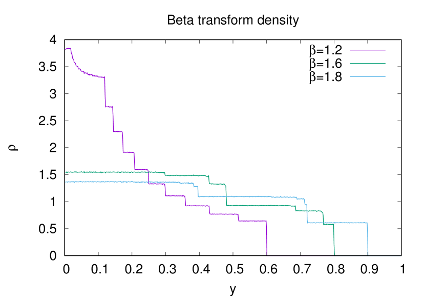
Figure 1: Beta-shift Density Distribution

The above figure shows three different density distributions, for $\rho_{1.2}(y)$, $\rho_{1.6}(y)$ and $\rho_{1.8}(y)$, calculated numerically. These are obtained by histogramming a large number of point trajectories, as described in the text. The small quantities of jitter are due to a finite number of samples. To generate this figure, a total of $M=4000$ iterations were performed, using randomly generated arbitrary-precision floats (using the Gnu GMP package), partitioned into $N=800$ bins, and sampled 24000 times (or 30 times per bin) to perform the averaging integral. It will later be seen that the discontinuities in this graph occur at the “iterated midpoints” $m_{p}=T_{\beta}^{p}\left(\beta/2\right)$. The flat plateaus are not quite flat, but are filled with microscopic steps. There is a discontinuous step at every $p$; these are ergodically distributed, i.e. dense in the interval, so that there are steps everywhere. This is the general case; for special cases, when the midpoint has a finite orbit, then there are a finite number of perfectly flat plateaus. The first such example occurs at $\beta=\left(1+\sqrt{5}\right)/2=\varphi$ the Golden Ratio. In this case, there are only two such plateaus.

 

The general trend of the distributions, as a function of $\beta$, can be visualized with a Feigenbaum-style “bifurcation diagram”, shown in figure 2. This color-codes each distribution $\rho_{\beta}(y)$ and arranges them in a stack; a horizontal slice through the diagram corresponds to $\rho_{\beta}(y)$ for a fixed value of $\beta$. A related visualization is in 3, which highlights the discontinuities in 2. Periodic orbits appear wherever the traceries in this image intersect. A characterization of these orbits occupies a large portion of this text.

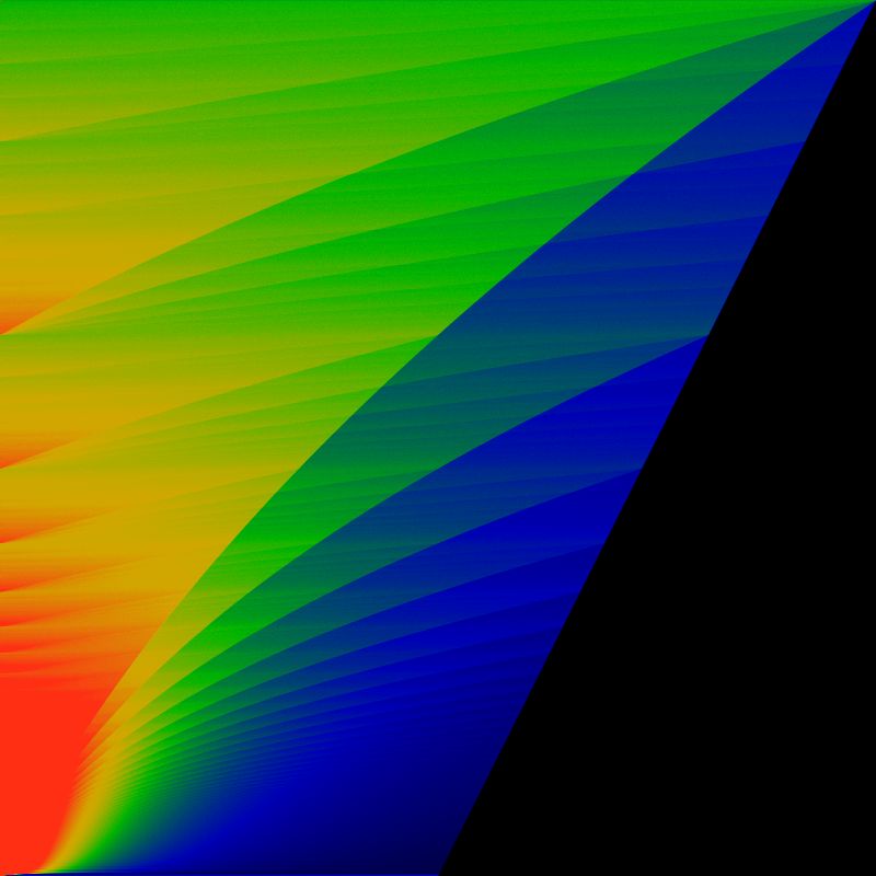
Figure 2: Beta-shift Bifurcation Diagram

This figure shows the density $\rho_{\beta}(y)$, rendered in color. The constant $\beta$ is varied from 1 at the bottom to 2 at the top; whereas $y$ runs from 0 on the left to 1 on the right. Thus, a fixed value of $\beta$ corresponds to a horizontal slice through the diagram. The color green represents values of $\rho_{\beta}(y)\approx 1.0$, while red represents $\rho_{\beta}(y)\gtrsim 2$ and blue-to-black represents $\rho_{\beta}(y)\apprle 0.5$. The lines forming the fan shape are not straight. The precise form is examined in a later section, given by a variant of the polynomial in eqn 7. The discontinuities in this figure are more clearly highlighted in the next figure, 3.

 

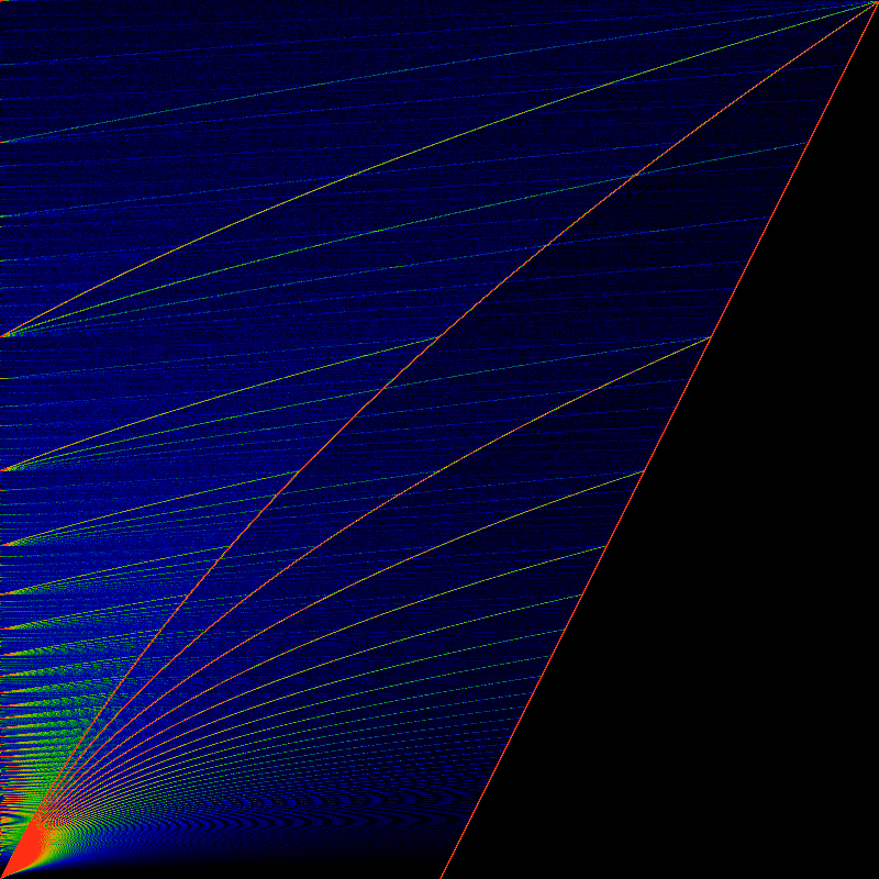
Figure 3: Midpoint Trace

Traces of midpoint iteration. Each horizontal line corresponds to a fixed $\beta$, with $\beta$ running fom 1 at the bottom, to 2 at the top. At each fixed $\beta$, the midpoint $x=1/2$ is iterated to generate $T_{\beta}^{n}(1/2)$. At each such location (from left to right, of 0 to 1), the corresponding pixel is given a color assignment, fading from red, through a rainbow, to black, as $n$ increases. This is a variant of 2, highlighting the edges. A formal analysis of the traceries begins with figure 11

 

1.8 Tent Map

The tent map is a closely related iterated map, given by iteration of the function

$$v_{\beta}(x)=\begin{cases}\beta x&\mbox{ for }0\leq x<\frac{1}{2}\\ \beta\left(1-x\right)&\mbox{ for }\frac{1}{2}\leq x\leq 1\end{cases}$$

Its similar to the beta shift, except that the second arm is reflected backwards, forming a tent. The bifurcation diagram is shown in figure 4. Its is worth contemplating the similarities between this, and the corresponding beta shift diagram. Clearly, there are a number of shared features.

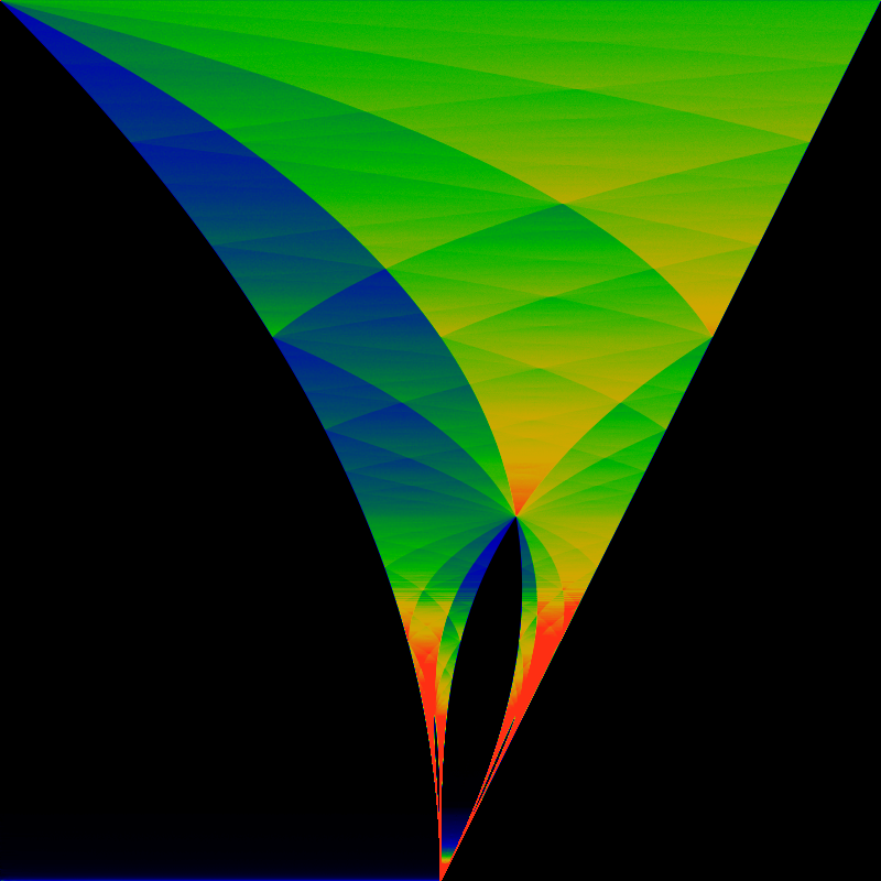
Figure 4: Tent Map Bifurcation Diagram

The bifurcation diagram for the tent map. The value of $\beta$ runs from 1 at the bottom of the image, to 2 at the top. The color scheme is adjusted so that green represents the average value of the distribution, red represents areas of more than double the average value, while blue shows those values that are about half the average value. Note that this is a different color scheme than that used in figure 2; that scheme would obliterate the lower half of this figure in red.

The black areas represent parts of the iterated range that are visited at most a finite number of times. To the right, the straight boundary indicates that after one iteration, points in the domain $\beta/2\leq x\leq 1$ are never visited. To the left, points in the domain $0\leq x\leq\beta\left(1-\beta/2\right)$ are never visited more than a finite number of times.

The figure can be imagined to be a superposition of a countable number of copies of figure 2, each drawn out so as to terminate in a point, but separated into distinct arms. Each copy is recapitulated in the Feigenbaum bifurcation diagram.

 

1.9 Logistic Map

The logistic map is related to the tent map, and is given by iteration of the function

$$f_{\beta}\left(x\right)=2\beta x(1-x)$$

It essentially replaces the triangle forming the tent map with a parabola of the same height. That is, the function is defined here so that the the same value of $\beta$ corresponds to the same height for all three maps. Although the heights of the iterators have been aligned so that they match, each exhibits rather dramatically different dynamics. The $\beta$-transform has a single fixed point for $\beta<1$, and then explodes into a fully chaotic regime above that. By contrast, the logistic map maintains a single fixed point up to $\beta=3/2$, where it famously starts a series of period-doubling bifurcations. The onset of chaos is where the bifurcations come to a limit, at $\beta=3.56995/2=1.784975$. Within this chaotic region are “islands of stability”, which do not appear in either the $\beta$-transform, or in the tent map. The tent map does show a period-doubling regime, but in this region, there are no fixed points: rather, the motion is chaotic, but confined to multiple arms. At any rate, the period doubling occurs at different values of $\beta$ than for the logistic map.

The bifurcation diagram is shown in figure 5. Again, it is worth closely examining the similarities between this, and the corresponding tent-map diagram, as well as the $\beta$-transform diagram. Naively, it would seem that the general structure of the chaotic regions are shared by all three maps. Thus, in order to understand chaos in the logistic map, it is perhaps easier to study it in the $\beta$-transform.

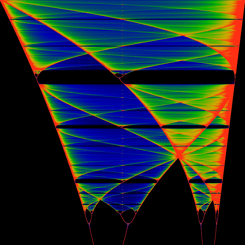
Figure 5: Logistic Map Bifurcation Diagram

The logistic map bifurcation diagram. The value of $\beta$ runs from 1.75 at the bottom of the image, to 2 at the top. The color scheme is adjusted so that green represents the average value of the distribution, red represents areas of more than double the average value, while blue shows those values that are about half the average value. Clearly, the orbits of the iterated points spend much of their time near the edges of the diagram.

This is a very widely reproduced diagram. The goal here is not to waste space reproducing it yet again, but to draw attention to the similarities between this diagram, and figure 4. The tent can be smoothly deformed into the parabola; doing so separates the multiple legs visible at the bottom of 4, with each leg becoming a bifurcation branch. The central point, where all legs come together, is preserved in both images. The curving arcs, highlighted in figure 3, are retained as well. The legs of 4 are chaotic regions, and remain so as the tent is deformed into a parabola. They are merely separated from one-another. The legs do not shrink to zero width.

 

The general visual similarity between the figures 2, 4 and 5 should be apparent, and one can pick out and find visually similar regions among these three illustrations. Formalizing this similarity is a bit harder, but it can be done: all three of these maps are topologically conjugate to one-another. This is perhaps surprising, but is based on the observation that the “islands of stability” in the logistic map are countable, and are in one-to-one correspondence with certain “trouble points” in the iterated beta transformation. These are in turn in one-to-one correspondence with rational numbers. With a slight distortion of the beta transformation, the “trouble points” can be mapped to the islands of stability, in essentially the same way that phase locking regions (Arnold tongues) appear in the circle map. This is examined in a later section; it is mentioned here only to whet the appetite.

1.10 Beta Transformation

After exactly one iteration of the beta shift, all initial points $\beta/2\leq x\leq 1$ are swept up into the domain $0\leq x<\beta/2$, and never leave. Likewise, the range of the iterated beta-shift is $0\leq x<\beta/2$. Thus, an alternative representation of the beta shift, filling the entire unit square, can be obtained by dividing both the domain and range by $\beta/2$ to obtain the function

$$t_{\beta}(u)=\begin{cases}\beta u&\mbox{ for }0\leq u<\frac{1}{\beta}\\ \beta u-1&\mbox{ for }\frac{1}{\beta}\leq u\leq 1\end{cases}$$ (8)

This can be written more compactly as $t_{\beta}\left(x\right)=\beta x\mod 1$. In this form, the function is named “the beta-transform”, written as the $\beta$-transformation, presenting a typesetting challenge to search engines when used in titles of papers. The orbit of a point $x$ in the beta-shift is identical to the orbit of a point $u=2x/\beta$ in the beta-transformation. Explicitly comparing to the beta-shift of eqn 4:

$$T_{\beta}^{n}\left(x\right)=\frac{\beta}{2}t_{\beta}^{n}\left(\frac{2x}{\beta}\right)$$ (9)

The beta-shift and the $\beta$-transformation are essentially the same function; this text works almost exclusively with the beta-shift, and is thus idiosyncratic, as it flouts the more common convention of working with the $\beta$-transformation. The primary reason for this is a historical quirk, as this text was started before the author became aware of the $\beta$-transformation.

After a single iteration of the tent map, a similar situation applies. After one iteration, all initial points $\beta/2\leq x\leq 1$ are swept up into the domain $0\leq x<\beta/2$. After a finite number of iterations, all points $0<x\leq\beta\left(1-\beta/2\right)$ are swept up, so that the remaining iteration takes place on the domain $\beta\left(1-\beta/2\right)<x<\beta/2$. It is worth defining a “sidetent” function, which corresponds to the that part of the tent map in which iteration is confined. It is nothing more than a rescaling of the tent map, ignoring those parts outside of the above domain that wander away. The sidetent is given by

$$s_{\beta}(u)=\begin{cases}\beta\left(u-1\right)+2&\mbox{ for }0\leq u<\frac{\beta-1}{\beta}\\ \beta\left(1-u\right)&\mbox{ for }\frac{\beta-1}{\beta}\leq u\leq 1\end{cases}$$

Performing a left-right flip on the side-tent brings it closer in form to the beta-transformation. The flipped version, replacing $u\to 1-u$ is

$$f_{\beta}(u)=\begin{cases}\beta u&\mbox{ for }0\leq u<\frac{1}{\beta}\\ 2-\beta u&\mbox{ for }\frac{1}{\beta}\leq u\leq 1\end{cases}$$

The tent map (and the flipped tent) exhibits fixed points (periodic orbits; mode-locking) for the smaller values of $\beta$. These can be eliminated by shifting part of the tent downwards, so that the diagonal is never intersected. This suggests the “sidetarp”:

$$a_{\beta}(u)=\begin{cases}\beta u&\mbox{ for }0\leq u<\frac{1}{\beta}\\ \beta\left(1-u\right)&\mbox{ for }\frac{1}{\beta}\leq u\leq 1\end{cases}$$

The six different maps under consideration here are depicted in figure 6. It is interesting to compare three of the bifurcation diagrams, side-by-side. These are shown in figure 7.

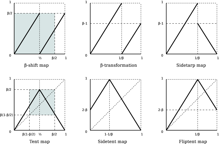
Figure 6: Iterated piece-wise linear maps

The beta shift map, shown in the upper left, generates orbits that spend all of their time in the shaded area: a box of size $\frac{\beta}{2}\times\frac{\beta}{2}$. Enlarging this box to the unit square gives the $\beta$-transformation. The tent map resembles the beta shift, except that one arm is flipped to make a tent-shape. After a finite number of iterations, orbits move entirely in the shaded region; enlarging this region to be the unit square gives the sidetent map. Flipping it left-right gives the fliptent map. Although it is not trivially obvious, the fliptent map and the sidetent map have the same orbits, and thus the same bifurcation diagram.

The bottom three maps all have prominent fixed points and periodic orbits, essentially because the diagonal intersects the map. The top three maps have periodic orbits, but these occur only for a countable number of $\beta$ values. General orbits are purely chaotic, essentially because the diagonal does not intersect them. Note that the slopes and the geometric proportions of all six maps are identical; they are merely rearrangents of the same basic elements.

 

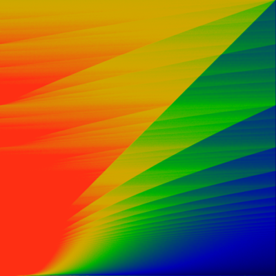
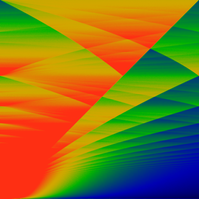
Figure 7: Beta transform and Side-tent

The left figure shows the bifurcation diagram for the $\beta$-transform, as it is normally defined as the $\beta x\mod 1$ map. It is the same map as the beta shift, just rescaled to occupy the entire unit square. In all other respects, it is identical to 2.

The middle figure is a similarly-rescaled tent map, given the name “side tent” in the main text. It is essentially identical to 4, with the middle parts expanded and the sides removed. In both figures, $\beta$ runs from 1 at the bottom to 2 at the top. The right-hand-side figure is the “sidetarp”, clearly its an oddly-folded variant of the beta transform.

 

1.11 Dynamical Systems

A brief review of dynamical systems is in order, as it provides a coherent language with which to talk about and think about the beta-shift. The technical reason for this is that a subshift $S\subset\left\{0,1\right\}^{\omega}$ provides a more natural setting for the theory, and that a lot of the confusion about what happens on the unit interval is intimately entangled with the homomorphism 3 (or 6 as the case may be). Disentangling the subshift from the homomorphism provides a clearer insight into what phenomena are due to which component.

The review of dynamical systems here is more-or-less textbook-standard material; it is included here only to provide a firm grounding for later discussion.

The Cantor space $\left\{0,1\right\}^{\omega}$ can be given a topology, the product topology. The open sets of this topology are called “cylinder sets”. These are the infinite strings in three symbols: a finite number of 0 and 1 symbols, and an infinite number of * symbols, the latter meaning “don’t care”. Set union is defined location-by-location, with $0\cup*=1\cup*=*$ and set intersection as $0\cap*=0$ and $1\cap*=1$. Set complement exchanges 0 and 1 and leaves * alone: $\overline{0}=1$, $\overline{1}=0$ and $\overline{*}=*$. The topology is then the collection of all cylinder sets. Note that the intersection of any finite number of cylinder sets is still a cylinder set, as is the union of an infinite number of them. The product topology does not contain any “points”: strings consisting solely of just 0 and 1 are not allowed in the topology. By definition, topologies only allow finite intersections, and thus don’t provide any way of constructing “points”. Of course, points can always be added “by hand”, but doing so tends to generate a topology (the “box topology”) that is “too fine”; in particular, the common-sense notions of a continuous function are ruined by fine topologies. The product topology is “coarse”.

The Borel algebra, or sigma-algebra, takes the topology and also allows set complement. This effectively changes nothing, as the open sets are still the cylinder sets, although now they are “clopen”, as they are both closed and open.

Denote the Borel algebra by $\mathcal{B}$. A shift is now a map $T:\mathcal{B}\to\mathcal{B}$ that lops off the leading symbol of a given cylinder set. This is provides strong theoretical advantages over working with “point dynamics”: confusions about counting points and orbits and defining densities go away. This is done by recasting discussion in terms of functions $f:\mathcal{B}\to\mathbb{R}$ from Borel sets to the reals (or the complex numbers $\mathbb{C}$ or other fields, when this is interesting). An important class of such functions are the measures. These are functions $\mu:\mathcal{B}\to\mathbb{R}$ that are positive, and are “compatible” with the sigma algebra, in that $\mu\left(A\cup B\right)=\mu\left(A\right)+\mu\left(B\right)$ whenever $A\cap B=\varnothing$ and (for product-space measures) that $\mu\left(A\cap B\right)=\mu\left(A\right)\mu\left(B\right)$ for all $A,B\in\mathcal{B}$. The measure of the total space $\Omega=\left\{0,1\right\}^{\omega}$ is by convention unity: $\mu\left(\Omega\right)=1$.

The prototypical example of a measure is the Bernoulli measure, which assigns probability $p$ to any string containing a single 0 and the rest all *’s. By complement, a string containing a single 1 and the rest all *’s has probability $1-p$. The rest follows from the sigma algebra: a cylinder set consisting of $m$ zeros and $n$ ones has measure $p^{m}\left(1-p\right)^{n}$. It is usually convenient to take $p=1/2$, the “fair coin”; the Bernoulli process is a sequence of coin tosses.

The map given in equation 3 is a homomorphism from the Cantor space to the unit interval. It extends naturally to a map from the Borel algebra $\mathcal{B}$ to the algebra of intervals on the unit interval. It is not an isomorphism: cylinder sets are both open and closed, whereas intervals on the real number line are either open, or closed (or half-open). It is convenient to take the map as a map to closed intervals, so that it’s a surjection onto the reals, although usually, this detail does not matter. What does matter is if one takes $p=1/2$, then the Bernoulli measure is preserved: it is mapped onto the conventional measure on the real-number line. Thus, the cylinder set $0***\cdots$ is mapped to the interval $\left[0,1/2\right]$ and $1***\cdots$ is mapped to $\left[1/2,1\right]$ and both have a measure of $1/2$ and this extends likewise to all intersections and unions. Points have a measure of zero. That is, the homomorphism 3 preserves the fair-coin Bernoulli measure.

Much of what is said above still holds for subshifts. Recall, a subshift $S$ is a subspace $S\subset\left\{0,1\right\}^{\omega}$ that is invariant under the shift $T$, so that $TS=S$. The space $S$ inherits a topology from $\left\{0,1\right\}^{\omega}$; this is the subspace topology. The Borel algebra $\mathcal{B}$ is similarly defined, as are measures. One can now (finally!) give a precise definition for an invariant measure: it is a measure $\mu$ such that $\mu\circ T^{-1}=\mu$, or more precisely, for which $\mu\left(T^{-1}\left(\sigma\right)\right)=\mu\left(\sigma\right)$ for almost all cylinder sets $\sigma\in S$. This is what shift invariance looks like. Note carefully that $T^{-1}$ and not $T$ is used in the definition. This is because $T^{-1}$ is a surjection while $T$ is not: every cylinder set $\sigma$ in the subshift “came from somewhere”; we want to define invariance for all $\sigma$ and not just for some of them.

The $T^{-1}$ is technically called a “pushforward”, and it defines a linear operator $\mathcal{L}_{T}$ on the space $\mathcal{F}$ of all functions $f:\mathcal{B}\to\mathbb{R}$. It is defined as $\mathcal{L}_{T}:\mathcal{F\to\mathcal{F}}$ by setting $\mathcal{L}_{T}:f\mapsto f\circ T^{-1}$. It is obviously linear, in that $\mathcal{L}_{T}\left(af+bg\right)=a\mathcal{L}_{T}\left(f\right)+b\mathcal{L}_{T}\left(g\right)$. This pushforward is canonically called the “transfer operator” or the “Ruelle-Frobenius-Perron operator”. Like any linear operator, it has a spectrum. The precise spectrum depends on the space $\mathcal{F}$.

The canonical example is again the Bernoulli shift. For this, we invoke the inverse of the mapping of eqn 3 so that $f:\left[0,1\right]\to\mathbb{R}$ is a function defined on the unit interval, instead of $f:\mathcal{B}\to\mathbb{R}$. When $\mathcal{F}$ is the space of real-analytic functions on the unit interval, that is, the closure of the space of all polynomials in $x\in\left[0,1\right]$, then the spectrum of $\mathcal{L}_{T}$ is discrete. It consists of the Bernoulli polynomials $B_{n}\left(x\right)$ corresponding to an eigenvalue of $2^{-n}$. That is,$\mathcal{L}_{T}B_{n}=2^{-n}B_{n}$. Note that $B_{0}\left(x\right)=1$ is the invariant measure on the full shift. For the space of square-integrable functions $f:\left[0,1\right]\to\mathbb{R}$, the spectrum of $\mathcal{L}_{T}$ is continuous, and consists of the unit disk in the complex plane; the corresponding eigenfunctions are fractal. Even more interesting constructions are possible; the Minkowski question mark function provides an example of a measure on $\left\{0,1\right\}^{\omega}$ that is invariant under the shift defined by the Gauss map $h\left(x\right)\mapsto\frac{1}{x}-\left\lfloor\frac{1}{x}\right\rfloor$. That is, as a measure, it solves $\mathcal{L}_{T}?^{\prime}=?^{\prime}$ with $?$ the Minkowski question mark function, and $?^{\prime}$ it’s derivative; note that the derivative is “continuous nowhere”. This rather confusing idea (of something being “continuous nowhere”) can be completely dispelled by observing that it is well-defined on all cylinder sets in $\mathcal{B}$ and is finite on all of them – not only finite, but less than one, as any good measure must obey.

These last examples are mentioned so as to reinforce the idea that working with $\mathcal{B}$ instead of the unit interval $\left[0,1\right]$ really does offer some strong conceptual advantages. They also reinforce the idea that the Bernoulli shift is not the only “full shift”. In the following text, we will be working with subshifts, primarily the beta-shift, but will draw on ideas from the above so as to make rigorous statements about measurability and invariance, without having to descend into either ad hoc hand-waving or provide painfully difficult (and confusing) reasoning about subsets of the real-number line.

1.12 Beta Transformation Literature Review and References

The $\beta$-transformation, in the form of $t_{\beta}\left(x\right)=\beta x\mod 1$ has been well-studied over the decades. The beta-expansion 5 was introduced by A. Renyi[Renyi57] in 1957, who demonstrates the existence of the invariant measure. The ergodic properties of the transform were proven by W. Parry[Parry60] in 1960, who also shows that the system is weakly mixing.

An explicit expression for the invariant measure was obtained independently by A.O. Gel’fond[Gelfond59] in 1959, and by W. Parry[Parry60], as a summation of step functions

$$\nu_{\beta}\left(y\right)=\frac{1}{F}\sum_{n=0}^{\infty}\frac{\varepsilon_{n}\left(y\right)}{\beta^{n}}$$ (10)

where $\varepsilon_{n}$ is the digit sequence

$$\varepsilon_{n}\left(y\right)=\begin{cases}1&\mbox{ if }y<t_{\beta}^{n}\left(1\right)\\ 0&\mbox{ otherwise}\end{cases}$$ (11)

and $F$ is a normalization constant. By integrating $\varepsilon_{n}\left(y\right)$ under the sum, the normalization is given by

$$F=\sum_{n=0}^{\infty}\frac{t_{\beta}^{n}\left(1\right)}{\beta^{n}}$$

Analogous to the way in which a dyadic rational $p/2^{n}$ has two different binary expansions, one ending in all-zeros, and a second ending in all-ones, so one may also ask if and when a real number $x$ might have more than one $\beta$-expansion (for fixed $\beta$). In general, it can; N. Sidorov shows that almost every number has a continuum of such expansions![Sidorov03] This signals that the beta shift behaves rather differently from the Cantor set in it’s embedding.

Conversely, the “univoke numbers” are those values of $\beta$ for which there is only one, unique expansion for $x=1$. These are studied by De Vries.[DeVries06]

The $\beta$-transformation has been shown to have the same ergodicity properties as the Bernoulli shift.[Dajani97] The fact that the beta shift, and its subshifts are all ergodic is established by Climenhaga and Thompson.[Clim10]

An alternative to the notion of ergodicity is the notion of universality: a $\beta$-expansion is universal if, for any given finite string of bits, that finite string occurs somewhere in the expansion. This variant of universality was introduced by Erdös and Komornik[Erdos98]. Its is shown by N. Sidorov that almost every $\beta$-expansion is universal.[Sidorov02] Conversely, there are some values of $\beta$ for which rational numbers have purely periodic $\beta$-expansions;[Adamczewski10] all such numbers are Pisot numbers.[Schmidt80]

The symbolic dynamics of the beta-transformation was analyzed by F. Blanchard[Blanchard89]. A characterization of the periodic points are given by Bruno Maia[Maia07]. A discussion of various open problems with respect to the beta expansion is given by Akiyama.[Akiyama09]

When the beta expansion is expanded to the entire real-number line, one effectively has a representation of reals in a non-integer base. One may ask about arithmetic properties, such as the behavior of addition and multiplication, in this base - for example, the sum or product of two $\beta$-integers may have a fractional part! Bounds on the lengths of these fractional parts, and related topics, are explored by multiple authors.[Guimond01, Julien06, Hbaib13]

Certain values of $\beta$ – generally, the Pisot numbers, generate fractal tilings,[Thurston89, Berthe05, Ito05, Adamczewski10, Akiyama09] which are generalizations of the Rauzy fractal. An overview, with common terminology and definitions is provided by Akiyama.[Akiyama17] The tilings, sometimes called (generalized) Rauzy fractals, can be thought of as living in a direct product of Euclidean and $p$-adic spaces.[Berthe04]

The set of finite beta-expansions constitutes a language, in the formal sense of model theory and computer science. This language is recursive (that is, decidable by a Turing machine), if and only if $\beta$ is a computable real number.[Simonsen11]

The zeta function, and a lap-counting function, are given by Lagarias[Lagarias94]. The Hausdorff dimension, the topological entropy and general notions of topological pressure arising from conditional variational principles is given by Daniel Thompson[Thompson10]. A proper background on this topic is given by Barreira and Saussol[Barreira01].

None of the topics or results cited above are made use of, or further expanded on, or even touched on in the following. This is not intentional, but rather a by-product of different goals.

2 Transfer operators

Given any map from a space to itself, mapping points to points, the pushforward maps distributions to distributions. The pushforward is a linear operator, called the transfer operator or the Ruelle–Frobenius–Perron operator. The spectrum of this operator, broken down into eigenfunctions and eigenvalues, can be used to understand the time evolution of a given density distribution. The invariant measure is an eigenstate of this operator, it is the eigenstate with eigenvalue one. There are other eigenstates; these are explored in this section.

Restricting to the unit interval, given an iterated map $f:\left[0,1\right]\to\left[0,1\right]$, the transfer operator acting on a distribution $\rho:\left[0,1\right]\to\mathbb{R}$ is defined as

$$\left[\mathcal{L}_{f}\rho\right]\left(y\right)=\sum_{x=f^{-1}(y)}\frac{\rho(x)}{\left|f^{\prime}(x)\right|}$$

The next subsection gives an explicit expression for this, when $f$ is the $\beta$-transform. After that, a subsection reviewing the invariant measure, and then a discussion of some other eigenfunctions.

2.1 The $\beta$-shift Transfer Operator

This text works primarily with the $\beta$-shift, instead of the more common $\beta$-transform. These two are more-or-less the same thing, differing only by scale factors, as given in eqn. 9. The transfer operators are likewise only superficially different, being just rescalings of one-another; both are given below.

The transfer operator the beta-shift map $T_{\beta}(x)$ is

$$\left[\mathcal{L}_{\beta}f\right]\left(y\right)=\begin{cases}\frac{1}{\beta}\left[f\left(\frac{y}{\beta}\right)+f\left(\frac{y}{\beta}+\frac{1}{2}\right)\right]&\mbox{ for }0\leq y\leq\beta/2\\ 0&\mbox{ for }\beta/2<y\leq 1\end{cases}$$

or, written more compactly

$$\left[\mathcal{L}_{\beta}f\right]\left(y\right)=\frac{1}{\beta}\left[f\left(\frac{y}{\beta}\right)+f\left(\frac{y}{\beta}+\frac{1}{2}\right)\right]\Theta\left(\frac{\beta}{2}-y\right)$$ (12)

where $\Theta$ is the Heaviside step function. The transfer operator for the beta-transform map $t_{\beta}(x)$ is

$$\left[\mathcal{M}_{\beta}f\right]\left(y\right)=\frac{1}{\beta}\left[f\left(\frac{y}{\beta}\right)+f\left(\frac{y}{\beta}+\frac{1}{\beta}\right)\Theta\left(\beta-1-y\right)\right]$$

The density distributions graphed in figure 1 are those functions satisfying

$$\left[\mathcal{L}_{\beta}\mu\right]\left(y\right)=\mu\left(y\right)$$ (13)

That is, the $\mu\left(y\right)$ satisfies

$$\mu\left(y\right)=\frac{1}{\beta}\left[\mu\left(\frac{y}{\beta}\right)+\mu\left(\frac{y}{\beta}+\frac{1}{2}\right)\right]\Theta\left(\frac{\beta}{2}-y\right)$$ (14)

Likewise, the Gelfond-Parry measure of eqn 10 satisfies

$$\left[\mathcal{M}_{\beta}\nu_{\beta}\right]\left(y\right)=\nu_{\beta}\left(y\right)$$

Recall that $\mu\left(y\right)=\frac{2}{\beta}\nu_{\beta}\left(\frac{2y}{\beta}\right)\Theta\left(\frac{\beta}{2}-y\right)$; the two invariant measures are just scaled copies of one-another. Both are normalized so that $\int_{0}^{1}\mu\left(y\right)dy=\int_{0}^{1}\nu_{\beta}\left(y\right)dy=1$.

Both of these invariant measures are the Ruelle-Frobenius-Perron (RFP) eigenfunctions of the corresponding operators, as they correspond to the largest eigenvalues of the transfer operators, in each case being the eigenvalue one.

More generally, one is interested in characterizing the spectrum

$$\left[\mathcal{L}_{\beta}\rho\right]\left(y\right)=\lambda\rho\left(y\right)$$

for eigenvalues $\left|\lambda\right|\leq 1$ and eigenfunctions $\rho\left(y\right)$. Solving this equation requires choosing a space of functions in which to work. Natural choices include piece-wise continuous smooth functions (piece-wise polynomial functions), any of the Banach spaces, and in particular, the space of square-integrable functions. In general, the spectrum will be complex-valued: eigenvalues will be complex numbers.

If a distribution $\rho\left(y\right)$ is nonzero on the interval $\left[\beta/2,1\right]$, the operator $\mathcal{L}_{\beta}$ will map it to one that is zero on this interval. Thus, it makes sense to restrict oneself to densities that are nonzero only on $\left[0,\beta/2\right]$. When this is done, eqn 12 has the slightly more convenient form

$$\left[\mathcal{L}_{\beta}f\right]\left(y\right)=\frac{1}{\beta}\left[f\left(\frac{y}{\beta}\right)\Theta\left(m_{0}-y\right)+f\left(\frac{y}{\beta}+\frac{1}{2}\right)\Theta\left(m_{1}-y\right)\right]$$

with $m_{0}=\beta/2$ and $m_{1}=\beta\left(\beta-1\right)/2=T_{\beta}\left(m_{0}\right)$. It is always the case that $m_{1}<m_{0}$ and so the second term above vanished on the interval $\left[m_{1},m_{0}\right]$. This can be gainfully employed in a variety of settings; typically to write $\mathcal{L}_{\beta}f$ on $\left[m_{1},m_{0}\right]$ as a simple rescaling of $\mathcal{L}_{\beta}f$ on $\left[0,m_{1}\right]$.

This equation can be treated as a recurrence relation; setting $\mathcal{L}_{\beta}f=f$ gives the $\lambda=1$ eigenstate. Performing this recursion gives exactly the densities shown in figure 1. Computationally, these are much cheaper to compute than trying to track a scattered cloud of points; the result is free of stochastic sampling noise. This density is the Ruelle–Frobenius–Perron eigenstate; an explicit expression was given by Gelfond and by Parry, as described in the next section.

2.2 The Gelfond–Parry measure

An explicit expression for the solution to $\mathcal{M}_{\beta}\nu=\nu$ was given by Gelfond[Gelfond59] and by Parry[Parry60]. It is the expression given by eqn 10. Unfortunately, I find the Russian original of Gelfond’s article unreadable, and Parry’s work, stemming from his PhD thesis, is not available online. Therefore, it is of some interest to provide a proof suitable for the current text. A generalization of this proof, stated in terms of a Borel algebra, is used in the subsequent section to construct general eigenfunctions.

There are two routes: either a direct verification that eqn 10 is correct, or a derivation of eqn 10 from geometric intuition. The direct verification is useful for practical purposes; the geometric construction, as a stretch-cut-stack map, provides insight. Both are given.

The Gelfond–Parry measure includes a normalization factor. It will be of recurring interest, and so a graph f it is presented in figure 8.

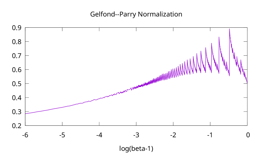
Figure 8: Gelfond–Parry Normalization

The above figure shows $1/F$ for the normalization constant $F=\sum_{n=0}^{\infty}t_{n}\beta^{-n}$ as a function of $\beta$. The horizonal axis is stretched out using $\log\left(\beta-1\right)$ so as to amplify the behavior as $\beta\to 1$. One has that $F\to\infty$ in this limit (so $1/F\to 0$); the curve suggests just how catastrophic that limit is. A graph of $F$ vs. $\beta$, without the rescaling of the horizontal axis, is shown in figure LABEL:fig:Normalization-Integral.

 

2.2.1 Direct verification

A direct verification of correctness is done below, explicitly showing all steps in laborious detail. It’s not at all difficult; just a bit hard on the eyes.

As before, let $t\left(x\right)\equiv t_{\beta}\left(x\right)=\beta x\mod 1$ be the $\beta$-transformation of eqn 8, and $t^{n}\left(x\right)$ the iterated transformation. Let $\Theta(x)$ be the Heaviside step function as always, and to keep notation brief, let $t_{n}\equiv t^{n}\left(1\right)$. The Gelfond-Parry measure is then

$$\nu\left(y\right)=\frac{1}{F}\sum_{n=0}^{\infty}\frac{\Theta\left(t_{n}-y\right)}{\beta^{n}}$$

where the normalization $F$ is given by

$$F=\sum_{n=0}^{\infty}\frac{t_{n}}{\beta^{n}}$$

The transfer operator $\mathcal{M}$ for the beta-transformation is slightly more convenient to work with than $\mathcal{L}$ for this particular case. It is given by

$$\left[\mathcal{M}f\right]\left(y\right)=\frac{1}{\beta}\left[f\left(\frac{y}{\beta}\right)+f\left(\frac{y+1}{\beta}\right)\Theta\left(\beta-1-y\right)\right]$$

and we wish to verify that $\mathcal{M}\nu=\nu$. Plugging in directly,

$$P=\nu\left(\frac{y}{\beta}\right) +\nu\left(\frac{y+1}{\beta}\right)\Theta\left(\beta-1-y\right)=$$

$$=\frac{1}{F}\sum_{n=0}^{\infty}\frac{1}{\beta^{n}}\left(\Theta\left(t_{n}-\frac{y}{\beta}\right)+\Theta\left(t_{n}-\frac{y+1}{\beta}\right)\Theta\left(\beta-1-y\right)\right)$$

$$=\frac{1}{F}\sum_{n=0}^{\infty}\frac{1}{\beta^{n}}\left(\Theta\left(\beta t_{n}-y\right)+\Theta\left(\beta t_{n}-1-y\right)\right)$$

The second line follows from the first, since $\Theta\left(ax\right)=\Theta\left(x\right)$ for all constants $a$, and the $\Theta\left(\beta-1-y\right)$ can be safely dropped, since $t_{n}\leq 1$ for all $n$. These terms simplify, depending on whether $t_{n}$ is small or large. Explicitly, one has

$$\Theta\left(\beta t_{n}-1-y\right)=0 \mbox{ if }\beta t_{n}-1<0$$

$$\Theta\left(\beta t_{n}-y\right)=1 \mbox{ if }\beta t_{n}-1>0$$

and so

$$P=\frac{1}{F}\sum_{n=0}^{\infty}\frac{1}{\beta^{n}}\left(\Theta\left(1-\beta t_{n}\right)\Theta\left(\beta t_{n}-y\right)+\Theta\left(\beta t_{n}-1\right)\left(1+\Theta\left(\beta t_{n}-1-y\right)\right)\right)$$

These can be collapsed by noting that

$$\beta t_{n}=t_{n+1} \mbox{ if }\beta t_{n}-1<0$$

$$\beta t_{n}-1=t_{n+1} \mbox{ if }\beta t_{n}-1>0$$

and so

$$P =\frac{1}{F}\sum_{n=0}^{\infty}\frac{1}{\beta^{n}}\left(\Theta\left(1-\beta t_{n}\right)\Theta\left(t_{n+1}-y\right)+\Theta\left(\beta t_{n}-1\right)\left(1+\Theta\left(t_{n+1}-y\right)\right)\right)$$

$$=\frac{1}{F}\sum_{n=0}^{\infty}\frac{1}{\beta^{n}}\left(\Theta\left(t_{n+1}-y\right)\left[\Theta\left(1-\beta t_{n}\right)+\Theta\left(\beta t_{n}-1\right)\right]+\Theta\left(\beta t_{n}-1\right)\right)$$

$$=\frac{1}{F}\sum_{n=0}^{\infty}\frac{1}{\beta^{n}}\left(\Theta\left(t_{n+1}-y\right)+\Theta\left(\beta t_{n}-1\right)\right)$$

$$=\beta\nu\left(y\right)-\frac{\beta}{F}+\frac{1}{F}\sum_{n=0}^{\infty}\frac{\Theta\left(\beta t_{n}-1\right)}{\beta^{n}}$$

$$=\beta\nu\left(y\right)$$

The last sum on the right is just the $\beta$-expansion for 1. That is, the $\beta$-expansion of $x$ is

$$x=\sum_{n=0}^{\infty}\frac{\Theta\left(\beta t^{n}\left(x\right)-1\right)}{\beta^{n+1}}$$

This is just eqn 6 written in a different way (making use of the equivalence 9). Thus $P=\beta\nu\left(y\right)$ and so $\mathcal{M}\nu=\nu$ as claimed.

2.2.2 Stretch–Cut–Stack Map

The measure can be geometrically constructed and intuitively understood as the result of the repeated application of a bakers-map-style stretch and squash operation. The idea is to iterate $\nu_{n+1}=\mathcal{M}_{\beta}\nu_{n}$, starting with $\nu_{0}=1$ and then take the limit $n\to\infty$; the result is $\nu_{n}\to\nu$ in the limit, given as above. The basic stretch-cut-stack operation provides intuition as to why $\nu$ is invariant. The proof that it converges as desired is nearly identical to the (shorter) proof above.

Consider a first approximation that $\nu_{0}$ is constant on the interval $\left[0,1\right]$, so that $\nu_{0}\left(y\right)=1$. The operation of $\mathcal{M}$ acting on this is to stretch it out to the interval $\left[0,\beta\right]$, chop off the $\left[1,\beta\right]$ part, move it to $\left[0,\beta-1\right]$, stack it on top, thus doubling the density in this region. The doubling, though, is partly counteracted by the stretching, which thins out the density to $1/\beta$ uniformly over the entire interval $\left[0,\beta\right]$. This operation preserves the grand-total measure on the unit interval. Writing $\beta-1=t_{1}=t\left(t_{0}\right)=t\left(1\right)$ for the first iterate of the endpoint $t_{0}=1$, this stretch, cut and stack operation should result in

$$\nu_{1}\left(y\right)=\begin{cases}\frac{2}{\beta}&\mbox{for }y\in\left[0,t_{1}\right]\\ \frac{1}{\beta}&\mbox{for }y\in\left[t_{1},t_{0}\right]\end{cases}$$

The stretch–cut–stack operation is the intuitive, geometrical explanation for obtaining the first iterate. The same result is obtained algebraically, by writing $\nu_{1}=\mathcal{M}\nu_{0}$ and then plugging and chugging:

$$\nu_{1}\left(y\right)=\frac{1}{\beta}\left[1+\Theta\left(t_{1}-y\right)\right]$$

The derivation of a recursive formula for $\nu_{n}$ follows along the line of the algebraic proof given in the previous section, this time, limiting the sums to finite order. The general form is

$$\nu_{n}=\rho_{n}-\sum_{k=0}^{n-1}c_{n-k}\nu_{k}$$

which is preserved under iteration as $\nu_{n+1}=\mathcal{M}\nu_{n}$. The two parts are $\rho_{n}$ defined as

$$\rho_{n}=\sum_{k=0}^{n}\frac{1}{\beta^{k}}\Theta\left(t_{k}-y\right)$$

This converges, up to overall normalization, to the invariant measure: $\rho_{n}\to F\nu$ with $F$ the normalization constant from before. The $c_{n}$ are constants, defined as

$$c_{n}=1-\sum_{k=0}^{n-1}\frac{\Theta\left(\beta t_{k}-1\right)}{\beta^{k+1}}$$ (15)

The sum in $c_{n}$ is a partial $\beta$-expansion for 1. Each term can be recognized as a bit from the bit-expansion:

$$\Theta\left(\beta t_{k}-1\right)=d_{n}\left(\frac{1}{2}\right)=k_{n}\left(\frac{\beta}{2}\right)=\varepsilon_{n}\left(\frac{1}{\beta}\right)$$

with $k_{n}$ as defined in eqn 5, $\varepsilon_{n}$ defined as in eqn 11 and $d_{n}$ as in eqn 19 (apologies for the variety of notations; each is “natural” in a specific context.) The $\beta$-expansion of a real number $x$ is as given in eqn 6. In the present context, this is the expansion for $x=\beta/2$, or, after rescaling, the expansion for $x=1$:

$$1=\sum_{k=0}^{\infty}\frac{\Theta\left(\beta t_{k}-1\right)}{\beta^{k+1}}$$

Thus, $\left|c_{n}\right|<\beta^{-n+1}$ and $c_{n}\to 0$ as $n\to\infty$. The sum in $c_{n}$ is a partial $\beta$-expansion for 1. Thus, $\left|c_{n}\right|<\beta^{-n+1}$ and $c_{n}\to 0$ as $n\to\infty$.

Each iteration preserves the measure; this is built into the construction. That is, $\int_{0}^{1}\nu_{n}\left(y\right)dy=1$ for all $n$. Plugging through gives a curious identity:

$$1=\int_{0}^{1}\nu_{n}\left(y\right)dy=\sum_{k=0}^{n}\frac{t_{k}}{\beta^{k}}-\sum_{k=1}^{n}c_{k}$$

which holds for all $n$. This is readily verified by further plugging through; the underlying identity is that

$$t_{n}=\beta^{n}c_{n}$$

This follows by noticing that each $\Theta\left(\beta t_{k}-1\right)$ records a decision to decrement, or not, the product $\beta t_{k}$ occurring in the iteration $t_{k+1}=\beta t_{k}\mod 1$.

The Gelfond–Parry normalization was the $n\to\infty$ limit of the first sum: $F=\sum_{k=0}^{\infty}\beta^{-k}t_{k}$.

2.2.3 Stacking Generic Functions

A slightly different calculation results if one works with an an arbitrary function $\nu_{0}\left(y\right)$. The iteration to obtain $\nu_{n}=\mathcal{M}^{n}\nu_{0}$ proceeds much as before, with only minor modifications needed to obtain the general form.

The trick is to track two distinct travellers: one that travels with $\Theta\left(t_{k}-y\right)$ and another that travels with the bitsequence $b_{k}=\Theta\left(\beta t_{k}-1\right)$. The general solution has the form

$$\nu_{n}\left(y\right) =a_{n}\left(y\right)+\sum_{k=1}^{n}h_{nk}\left(y\right)\Theta\left(t_{k}-y\right)$$

$$a_{n}\left(y\right) =\sum_{k=0}^{n-1}b_{k}e_{nk}\left(y\right)$$ (16)

The functions $h_{nk}$ and $e_{nk}$ can be solved for recursively; the recursive relations are simple enough that they can be rolled up as series summations. These are given by

$$h_{nk}\left(y\right) =\frac{1}{\beta^{k}}a_{n-k}\left(t_{1}-\frac{\beta t_{k}-1}{\beta^{k}}+\frac{y}{\beta^{k}}\right)\quad\mbox{ for }n\geq k$$

which express $h_{nk}$ in terms of the function $a_{n}$. This is given as a recursive series, obtained by iterating

$$e_{nk}\left(y\right)=\frac{1}{\beta^{n}}\left[\nu_{0}\left(1-\frac{t_{k}}{\beta^{k}}+\frac{y}{\beta^{n}}\right)+\Theta\left(k\right)\sum_{m=1}^{n-k-1}\beta^{m}a_{m}\left(t_{1}-\frac{\beta t_{k}-1}{\beta^{k}}+\frac{\beta^{m}y}{\beta^{n}}\right)\right]$$

The starting point for iteration is $a_{0}=\nu_{0}$.

The function $a_{n}$ is polynomial if $\nu_{0}$ is, and of the same degree; $a_{n}$ is analytic, if $\nu_{0}$ is, and so on. The function $h_{nk}$ is likewise, on the domain $0\leq y\leq t_{k}$; the discontinuities in $\nu_{n}$ are entirely due to the $\Theta\left(t_{k}-y\right)$ term.

The proper calculation of the $n\to\infty$ limit of $a_{n}$ remains a mystery. This is the primary obstacle to constructing general eigenfunctions from this series.

Verification

When $\nu_{0}=1$, all three functions $a_{n},e_{nk}$ and $h_{nk}$ become constants. In this case, $a_{n}\to 1/F$ as $n\to\infty$, with $F$ the normalization constant as before. Defining $\alpha_{n}=\beta^{n}a_{n}$, the recursion relation takes the curious form

$$\alpha_{n}=1+\sum_{k=1}^{n-1}b_{k}\sum_{m=0}^{n-k-1}\alpha_{m}$$

This is an integer sequence: each $\alpha_{n}$ is an integer, starting with $\alpha_{0}=\alpha_{1}=1$. This has the form of a generalized Fibonacci sequence. Denote the partial sum as $s_{i}=\sum_{m=0}^{i}\alpha_{m}$. This implies $\alpha_{i}=s_{i}-s_{i-1}$ and so

$$\alpha_{n} =1+b_{1}s_{n-2}+b_{2}s_{n-3}+\cdots$$

$$s_{n} =1+s_{n-1}+b_{1}s_{n-2}+b_{2}s_{n-3}+\cdots$$

If the orbit is of finite length $p$, so that $b_{k}=0$ for $k>p$, then this can be recast directly into generalized Fibonacci form, by defining $f_{n}=s_{n}+\sum_{k=1}^{p}b_{k}$. The recursion relation is then

$$f_{n}=f_{n-1}+b_{1}f_{n-2}+\cdots+b_{p}f_{n-p}$$

For example, the orbit generated by $\beta=\varphi=1.618\cdots$ the golden mean has $p=1,b_{1}=1$ and the sequence is $\alpha_{m}=1,1,2,3,5,8,13,\cdots$. Finite orbits and generalized Fibonacci sequences will be treated at length in the next chapter. One of the interesting properties is that $\beta=\lim_{n\to\infty}f_{n}/f_{n-1}$ holds in the general case, and not just for the golden mean. The bitsequences are self-describing; this is byproduct from the identity $\beta=\sum_{k=0}^{\infty}b_{k}\beta^{-k}$.

2.2.4 Scaled iteration

It is convenient to rescale the iterate $\mathcal{M}^{n}$ by a constant factor, so that instead, one is examining a sequence of functions $\mathcal{M}\mu_{n}=\lambda\mu_{n+1}$. The iterated operator then has the form

$$\mu_{n}\left(y\right) =c_{n}^{\prime}\left(y\right)+\sum_{k=1}^{n}\frac{\Theta\left(t_{k}-y\right)}{\left(\lambda\beta\right)^{k}}c_{n-k}^{\prime}\left(t_{1}-\frac{\beta t_{k}-1}{\beta^{k}}+\frac{y}{\beta^{k}}\right)$$

$$c_{n}^{\prime}\left(y\right) =\nu_{0}\left(y\right)+\frac{1}{\left(\lambda\beta\right)^{n}}\sum_{k=1}^{n-1}b_{k}\left[\nu_{0}\left(1-\frac{t_{k}}{\beta^{k}}+\frac{y}{\beta^{n}}\right)+\sum_{m=1}^{n-k-1}\left(\lambda\beta\right)^{m}c_{m}^{\prime}\left(t_{1}-\frac{\beta t_{k}-1}{\beta^{k}}+\frac{\beta^{m}y}{\beta^{n}}\right)\right]$$

This is identical to the earlier forms when $\lambda=1$. The starting point for iteration is $c_{0}^{\prime}=\nu_{0}$. For For $\nu_{0}=1$ and $\lambda=1$, one regains the Gelfond–Parry distribution in the limit of $n\to\infty$. In this limit, $c_{n}^{\prime}\to 1/F$.

2.3 Analytic Gelfond–Parry function

The technique above can be repeated verbatim for a “rotated” or “coherent” function

$$\nu_{\beta;z}\left(y\right)=\sum_{n=0}^{\infty}z^{n}\frac{\Theta\left(t_{n}-y\right)}{\beta^{n}}$$ (17)

for a given complex-valued $z$. No changes are required, and the result can be read off directly:

$$\left[\mathcal{M}\nu_{\beta;z}\right]\left(y\right) =\frac{\nu_{\beta;z}\left(y\right)}{z}-\frac{1}{z}+\sum_{n=0}^{\infty}z^{n}\frac{\Theta\left(\beta t_{n}-1\right)}{\beta^{n+1}}$$

$$=\frac{\nu_{\beta;z}\left(y\right)}{z}+C\left(\beta;z\right)$$

with $C\left(\beta;z\right)$ being a constant independent of $y$. If there are values of $\beta$ and/or $z$ at which $C\left(\beta;z\right)=0$, then this becomes the eigenequation for $\mathcal{M}$.

The eigenfunction for $\mathcal{L}$ is the same, up to rescaling of $y\mapsto\beta x/2$. Recycling notation slightly, write

$$v_{\beta;z}\left(x\right)=\sum_{n=0}^{\infty}\frac{d_{n}\left(x\right)}{\beta^{n}}z^{n}$$ (18)

where the $d_{n}\left(x\right)$ are exactly the same digits as defined by Parry, just rescaled for the beta-shift. That is,

$$d_{n}\left(x\right)=\varepsilon_{n}\left(\frac{2x}{\beta}\right)=\Theta\left(\frac{\beta}{2}t_{n}-x\right)=\Theta\left(T^{n}\left(\frac{\beta}{2}\right)-x\right)=\begin{cases}1&\mbox{if }x<T^{n}\left(\frac{\beta}{2}\right)\\ 0&\mbox{otherwise}\end{cases}$$ (19)

where $T$ the beta-shift map of eqn 4 and eqn 9 is used. The iterated end-point becomes the iterated midpoint:

$$t^{n}\left(1\right)=\frac{2}{\beta}T^{n}\left(\frac{\beta}{2}\right)$$

Holding both $\beta$ and $x$ fixed, the summation is clearly convergent (and holomorphic in $z$) for complex numbers $z$ within the disk $\left|z\right|<\beta$. The eigenequation has the same form:

$$\left[\mathcal{L}_{\beta}v_{\beta;z}\right]\left(x\right)=\frac{1}{z}v_{\beta;z}\left(x\right)+C\left(\beta;z\right)$$

where $C\left(\beta;z\right)$ is a constant independent of $x$. Numeric verification reveals we were a bit glib: $C\left(\beta;z\right)$ is a constant for $x\leq\beta/2$ and is zero otherwise! (This is normal; $\mathcal{L}$ was defined in such a way that it is always exactly zero for $x>\beta/2$.)

The interesting limit is where $\left|z\right|\to\beta$ and so its convenient to re-express $C$ in terms of $\zeta=z/\beta$, so that everything is mapped to the unit disk. With some rearrangements, one obtains

$$E\left(\beta;\zeta\right)\equiv\zeta\beta C\left(\beta;\zeta\beta\right)=-1+\zeta\sum_{n=0}^{\infty}\zeta^{n}d_{n}\left(\frac{1}{2}\right)$$ (20)

Given that $d_{n}\left(1/2\right)=\Theta\left(\beta t_{n}-1\right)$, the above can be recognized as the rotated/coherent form of eqn 15 in the $n\to\infty$ limit. The primary task is to characterize the zeros of $E\left(\beta;\zeta\right)$. This is a straight-forward sum to examine numerically; results will be presented in the section after the next.

2.4 Analytic ergodics

This section proposes that the entire $\beta$-subshift can be tied together with a single holomorphic equation. The holomorphic equation effectively provides a continuum (i.e. uncountable number) of distinct relationships between different parts of the subshift. This can be interpreted either as a form of interaction across the subshift, or as a kind of mixing. Given the nature of the relationship, the moniker of “fundamental theorem of analytic ergodics” is an amusing name to assign to the result.

The constant term can be independently derived through a different set of manipulations. Explicitly plugging in eqn 18 into the transfer operator yields

$$C\left(\beta;z\right)= \left[\mathcal{L}_{\beta}v_{\beta;z}\right]\left(y\right)-\frac{v_{\beta;z}\left(y\right)}{z}$$

$$= \sum_{n=0}^{\infty}\frac{z^{n}}{\beta^{n}}\left[\frac{1}{\beta}\left[d_{n}\left(\frac{y}{\beta}\right)+d_{n}\left(\frac{y}{\beta}+\frac{1}{2}\right)\right]\Theta\left(\frac{\beta}{2}-y\right)-\frac{1}{z}d_{n}\left(y\right)\right]$$

Replacing $z$ by $\zeta=z/\beta$ gives

$$E\left(\beta;\zeta\right)= \zeta\beta C\left(\beta;\zeta\beta\right)$$

$$= \sum_{n=0}^{\infty}\zeta^{n}\left[\zeta\left[d_{n}\left(\frac{y}{\beta}\right)+d_{n}\left(\frac{y}{\beta}+\frac{1}{2}\right)\right]\Theta\left(\frac{\beta}{2}-y\right)-d_{n}\left(y\right)\right]$$

This is holomorphic on the unit disk $\left|\zeta\right|<1$, as each individual $d_{n}$ is either zero or one; there won’t be any poles inside the unit disk. Note that $d_{n}\left(y\right)=0$ for all $y>\beta/2$, and so one may pull out the step function to write

$$E\left(\beta;\zeta\right)=\sum_{n=0}^{\infty}\zeta^{n}\left[\zeta d_{n}\left(\frac{y}{\beta}\right)+\zeta d_{n}\left(\frac{y}{\beta}+\frac{1}{2}\right)-d_{n}\left(y\right)\right]\Theta\left(\frac{\beta}{2}-y\right)$$

confirming the earlier observation that $E\left(\beta;\zeta\right)$ vanishes for all $y>\beta/2$.

The bottom equation holds without assuming that $E\left(\beta;\zeta\right)$ is independent of $y$. However, we’ve already proven that it is; and so a simplified expression can be given simply by picking a specific $y$. Setting $y=0$, noting that $d_{n}\left(0\right)=1$ and canceling terms, one obtains eqn. 20 again.

Staring at the right-hand side of the sum above, it is hardly obvious that it should be independent of $y$. In a certain sense, this is not “one equation”, this holds for a continuum of $y$, for all $0\leq y\leq 1$. It is an analytic equation tying together the entire subshift. For each distinct $y$, it singles out three completely different bit-sequences out of the subshift, and ties them together. It is a form of mixing. Alternately, a form of interaction: the bit-sequences are not independent of one-another; they interact. This section attempts to make these notions more precise.

The tying-together of seemingly unrelated sequences seems somehow terribly important. It is amusing to suggest that this is a kind of “fundamental theorem of analytic ergodics”.

For such a claim, it is worth discussing the meaning at length, taking the effort to be exceptionally precise and verbose, perhaps a bit repetitive. Equation 4 defined a map, the $\beta$-shift. Equation 5 defined a bit-sequence, the $\beta$-expansion of a real number $0\leq x\leq 1$, where equation 6 is the definition of the $\beta$-expansion. The set of all such bit-sequences defines the shift. To emphasize this point, its best to compare side-by-side. Copying equation 5, one bitsequence records the orbit of $x$ relative to the midpoint:

$$k_{n}\left(x\right)=\begin{cases}0&\mbox{ if }0\leq T_{\beta}^{n}(x)<\frac{1}{2}\\ 1&\mbox{ if }\frac{1}{2}\leq T_{\beta}^{n}(x)\leq 1\end{cases}$$

while a different bitsequence records the orbit of the midpoint, relative to $x$:

$$d_{n}\left(x\right)=\begin{cases}1&\mbox{if }x<T^{n}\left(\frac{\beta}{2}\right)=T^{n+1}\left(\frac{1}{2}\right)\\ 0&\mbox{otherwise}\end{cases}$$

The iterations are running in opposite directions; this is as appropriate, since the the transfer operator was a pushforward.

It is useful to return to the language of sigma algebras and cylinder sets, as opposed to point dynamics. Recall that the Borel algebra $\mathcal{B}$ was defined as the sigma algebra, the collection of all cylinder sets in the product topology of $\left\{0,1\right\}^{\omega}$. A subshift is a subset $\mathcal{S}\subset\mathcal{B}$ together with a map $T:\mathcal{S}\to\mathcal{S}$ that lops off the leading symbol of a given cylinder set but otherwise preserves the subshift: $T\mathcal{S}=\mathcal{S}$. The inverted map $T^{-1}$ is a pushforward, in that it defines the transfer operator, a linear operator $\mathcal{L}_{T}:\mathcal{F\to\mathcal{F}}$ on the space $\mathcal{F}$ of all functions $f:\mathcal{S}\to\mathbb{R}$; explicitly, it is given by $\mathcal{L}_{T}:f\mapsto f\circ T^{-1}$. Insofar as the $d_{n}$ arose in the exploration of the transfer operator, it is not surprising that the shift is acting “backwards”.

The problem with the language of point dynamics is that one cannot meaningfully write $T^{-n}\left(x\right)$ for a real number, a point $x$, at least, not without severe contortions that lead back to the Borel algebra. Not for lack of trying; the $T^{-n}\left(x\right)$ is called the “Julia set” (to order $n$) of $x$: it is the preimage, the set of all points that, when iterated, converge onto $x$.

Can the analytic relation be restated in terms of cylinder sets? Yes, and it follows in a fairly natural way. The first step is to extend $d_{n}$ to a map $d_{n}:\mathcal{S}\to\left[0,1\right]$ into the unit interval, as opposed to being a single bit. Let $\mu:\mathcal{B}\to\left[0,1\right]$ be the canonical Bernoulli measure. Using the Bernoulli mapping 3, the interval $\left[0,T^{n}\left(\beta/2\right)\right]$ maps to some cylinder; call it $\Delta_{n}$. Then, given some cylinder $A\in\mathcal{S}$, define

$$d_{n}\left(A\right)=\mu\left(A\cap\Delta_{n}\right)$$

The rotated (pre-)measure is extended likewise:

$$\nu\left(A\right)=\sum_{n=0}^{\infty}\zeta^{n}d_{n}\left(A\right)$$

with $\zeta=z/\beta$ as before, recovering the Parry measure by setting $z=1$.

The Parry measure should be invariant under the action of $T^{-1}:\mathcal{S}\to\mathcal{S}$, and otherwise yield eqn 20. Let’s check. The proof will mirror the one of the previous section. Again, it is convenient to use the $\beta$-transform $t_{\beta}$ instead of the $\beta$-shift $T_{\beta}$. This is primarily a conceptual convenience; the subshift is more easily visualized in terms of the mod 1 map. Otherwise, the same notation is used, but rescaled, so that $\Delta_{n}$ is the cylinder corresponding to the interval $\left[0,t^{n}\left(1\right)\right]$.

Recall that for every $A\in\mathcal{S}$ and every $y\in A$, one will find that $y/\beta\in t^{-1}\left(A\right)$ and, whenever $y\leq\beta-1$ that also $\left(y+1\right)/\beta\in t^{-1}\left(A\right)$. Thus, $t^{-1}\left(A\right)$ naturally splits into two parts: the cylinder that maps to $\left[0,1/\beta\right]$, call it $D$, and the complement $\overline{D}$.

The pushforward action is then

$$\nu\left(t^{-1}\left(A\right)\right)= \sum_{n=0}^{\infty}\zeta^{n}\mu\left(\Delta_{n}\cap t^{-1}\left(A\right)\right)$$

$$= \sum_{n=0}^{\infty}\zeta^{n}\left[\mu\left(\Delta_{n}\cap D\cap t^{-1}\left(A\right)\right)+\mu\left(\Delta_{n}\cap\overline{D}\cap t^{-1}\left(A\right)\right)\right]$$

Two distinct cases emerge. When $t^{n}\left(1\right)<1/\beta$ then one has that $\Delta_{n}\cap\overline{D}=\varnothing$. Thus, the second term can be written as

$$\mu\left(\Delta_{n}\cap\overline{D}\cap t^{-1}\left(A\right)\right) =\Theta\left(t_{n}-\frac{1}{\beta}\right)\mu\left(\Delta_{n}\cap\overline{D}\cap t^{-1}\left(A\right)\right)$$

$$=\Theta\left(t_{n}-\frac{1}{\beta}\right)\frac{1}{\beta}\mu\left(\Delta_{n+1}\cap A\right)$$

where the second line follows from the first by linearity, and that $\overline{D}$ selected out one of the two branches of $t^{-1}\left(A\right)$. Meanwhile, when $t^{n}\left(1\right)>1/\beta$, then $D\subset\Delta_{n}$ so that $D\cap\Delta_{n}=D$. Thus, the first term splits into two:

$$\Theta\left(t_{n}-\frac{1}{\beta}\right)\mu\left(\Delta_{n}\cap D\cap t^{-1}\left(A\right)\right) =\Theta\left(t_{n}-\frac{1}{\beta}\right)\mu\left(D\cap t^{-1}\left(A\right)\right)$$

$$=\Theta\left(t_{n}-\frac{1}{\beta}\right)\frac{1}{\beta}\mu\left(A\right)$$

while

$$\Theta\left(\frac{1}{\beta}-t_{n}\right)\mu\left(\Delta_{n}\cap D\cap t^{-1}\left(A\right)\right)=\Theta\left(\frac{1}{\beta}-t_{n}\right)\frac{1}{\beta}\mu\left(\Delta_{n+1}\cap A\right)$$

Reassembling these pieces and making use of $\Delta_{0}\cap A=A$ one gets

$$\nu\left(t^{-1}\left(A\right)\right) =\sum_{n=0}^{\infty}\frac{\zeta^{n}}{\beta}\left[\mu\left(A\right)\Theta\left(t_{n}-\frac{1}{\beta}\right)+\mu\left(\Delta_{n+1}\cap A\right)\right]$$

$$=\frac{1}{z}\nu\left(A\right)-\frac{\mu\left(A\right)}{z}+\mu\left(A\right)\sum_{n=0}^{\infty}\frac{\zeta^{n}}{\beta}\Theta\left(t_{n}-\frac{1}{\beta}\right)$$

$$=\frac{1}{z}\nu\left(A\right)+\frac{\mu\left(A\right)}{z}E\left(\beta;z\right)$$

with the constant term as before, in eqn 20:

$$E\left(\beta;z\right) =-1+\zeta\sum_{n=0}^{\infty}\zeta^{n}\Theta\left(t_{n}-\frac{1}{\beta}\right)$$

$$=-1+\zeta\sum_{n=0}^{\infty}\zeta^{n}d_{n}\left(\frac{1}{2}\right)$$

As before, one has for $z=1$ that $E\left(\beta;1\right)=0$ and so $\nu\circ t^{-1}=\nu$ is indeed the measure invariant under $t^{-1}$. Other eigenvalues can be found for those values of $z$ for which $E\left(\beta;z\right)=0$. The task at hand is then to characterize $E\left(\beta;z\right)$.

2.5 Exploring $E\left(\beta;z\right)$

The function is easily explored numerically. It is clearly convergent in the unit disk $\left|\zeta\right|<1$ and has no poles in the disk. For almost all $\beta$, there seem to be a countable number of zeros within the disk, accumulating uniformly on the boundary as $\left|\zeta\right|\to 1$. An example is shown in figure 10. The notion of “uniformly” will be made slightly more precise in the next section, where it is observed that, for certain special values of $\beta$, the bit-sequence $d_{n}\left(\frac{1}{2}\right)$ is periodic, and thus is a polynomial. When it is polynomial, there are a finite number of zeros (obviously; the degree of the polynomial), which are distributed approximately uniformly near the circle $\left|\zeta\right|=1$. As the degree of the polynomial increases, so do the number of zeros; but they remain distributed approximately evenly. In this sense, the limit of infinite degree seems to continue to hold.

A handful of selected zeros are listed in the table below. The numbers are accurate to about the last decimal place.

$\beta$	$z$	$\left|z\right|$	$1/z$
1.8	-1.591567859	1.59156785	-0.6283112558
1.8	-1.1962384 +i 1.21602223	1.70578321	-0.41112138 - i 0.41792066
1.8	0.99191473 +i 1.44609298	1.75359053	0.32256553 -i 0.47026194
1.6	-1.06365138 +i 1.00895989	1.46606764	-0.49487018 -i 0.46942464
1.4	0.55083643 +i 1.17817108	1.30057982	0.32564816 -i 0.69652119
1.2	0.95788456 +i 0.60733011	1.13419253	0.74462841 -i -0.47211874

These are not particularly meaningful numbers; they just give a flavor for some locations of eigenvalues. Given a zero, the corresponding eigenfunction is also very easily computed. A typical eigenfunction is shown in figure 9; this is for the zero listed in the last row of the table above. Although it is unlike the figure 1, in that it is not strictly decreasing, it does have the same general plateau-like regions. Note that all such eigenfunctions are bounded and generally, differentiable-nowhere.

Figure 9: Typical Eigenfunction

A typical eigenfunction $v_{\beta;z}\left(x\right)$ solving $\mathcal{L}_{\beta}v=\lambda v$ for $\beta=1.2$. This is the eigenfunction is as defined in eqn 18. This eigenfunction corresponds to the zero $z=1.1342\exp i\pi 0.1799$ of $E\left(\beta;z\right)$, alternately of $C\left(\beta;z\right)$, as defined in eqn 20. The eigenvalue is $\lambda=1/z$. Since the eigenvalue is complex, so is the eigenfunction. The real and imaginary parts are paired in a way that vaguely resembles sine and cosine; such phased offsets are generic.

 

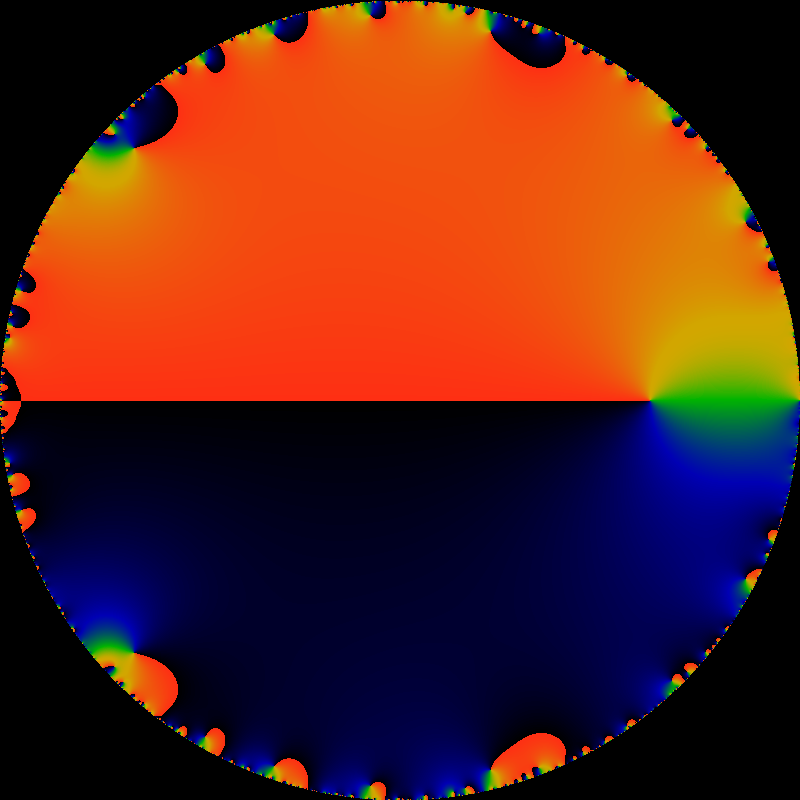
Figure 10: Disk of $E\left(\beta;z\right)$

The above shows a visualization of $E\left(\beta;z\right)$ for $\beta=1.6$ in the complex $\zeta=z/\beta$ plane. The disk consists of all $\zeta$ values with $\left|\zeta\right|\leq 1$. The plot is a phase plot, showing the argument $\arg E\left(\beta;z\right)\in\left[-\pi,\pi\right]$. The color-coding of blue-black puts the phase just above $-\pi$, green near 0, and red just below $+\pi$. Locations where the phase wraps around counter-clockwise (right-handed) are zeros of $E\left(\beta;z\right)$; this follows from Cauchy’s principle. The most prominent zero at the right-hand side of the image corresponds to $z=1$, located at $\zeta=1/\beta$ so well inside the circle. This corresponds to the Gelfond–Parry invariant measure. Other zeros are seen at the end of black-red whiskers, wrapping through green. These accumulate at the $\zeta=1$ boundary; in general, there are a countable number of such zeros. The corresponding eigenvalues are located at $\lambda=1/z=1/\beta\zeta$, so the accumulation ring of zeros occurs at $\left|\lambda\right|=1/\beta$.

 

As the zeros accumulate onto the circle $\left|\zeta\right|\to 1$, there appears to be no way to holomorphically continue the function $E\left(\beta;z\right)$ outside of the unit circle. This indicates that there is a lower bound on the possible eigenvalues that can be reached via the eigenfunctions of eqn 18. The lower bound is $\left|\lambda\right|=1/\beta$; the eigenfunctions with smaller eigenvalue do not arise from eqn 18.

The apparent reason for this is that the coherent state was constructed as a deformed version of the repeated iteration of $\nu_{0}=1$ a constant, as described in earlier sections. Iterating on $\nu_{0}\left(y\right)$ a polynomial appears to generate eigenfunctions with eigenvalue bounded by $1/\beta^{p}$ for a polynomial of degree $p$. One explicit example, generated by a parabola, is given in the next section. A simple, direct construction remains elusive.

A different derivation of this same holomorphic form will be given in the next chapter. There, the beta shift is shown to be conjugate to an infinite shift matrix, in explicit upper-Hessenberg form. Thus, the shift is explicitly a shift on the monomials $\zeta^{n}$ as the basis elements.

2.6 Other eigenfunctions

Eigenfunctions with eigenvalues $\lambda$ less than $1/\beta$ clearly exist. Below is an example with $\lambda=1/\beta^{2}$ for $\beta=\varphi=1.618\cdots$ the golden mean. It appears that similar constructions can be performed for any value of $\beta$ corresponding to a finite length orbit. Despite this, exhibiting an explicit form remains difficult, verbose and unsatisfactory. A precise and compact description is desirable, but remains undiscovered. Turgid details can be found in the research diary accompanying this text.

2.6.1 Piecewise quadratic eigenfuntions

To portray the problem, a piece-wise parabolic presentation is pursued. For $\beta=\varphi$, the function

$$\rho\left(y\right) =\begin{cases}\varphi y^{2}-y+\frac{1}{8}&\mbox{for }0\leq y<\frac{1}{2}\\ y^{2}-y+\frac{\varphi}{8}&\mbox{for }\frac{1}{2}\leq y<\frac{\varphi}{2}\\ 0&\mbox{for }\frac{\varphi}{2}\leq y\leq 1\end{cases}$$

satisfies $\mathcal{L}_{\varphi}\rho=\lambda\rho$ for $\lambda=\varphi^{-2}$.

2.6.2 Quasi-resonances

Returning to the expression for $\mathcal{M}\mu_{n}=\mu_{n+1}$ given in section 2.2.4, one might search for resonances by hypothesizing $\mu_{0}$ to be some polynomial, and then look for sequences $\lambda^{n}\mu_{n}\to\mu$ that converge uniformly in the $n\to\infty$ limit. Performing such a search reveals surprises. The following was observed.

Fix $\beta=1.6$. Then:

• If $\mu_{0}\left(x\right)=x-1/2$ then $\mu_{n}$ converges to $\approx-0.0869229\,\nu$ with $\nu$ the Gelfond–Parry invariant measure.

• If $\mu_{0}\left(x\right)=x-1/2+0.0869229$ (so that the convergent above is subtracted), then the $\mu_{n}$ appear to bounce around ergodically, maintaining a bounded norm. Three behaviors are apparent: $\beta^{n}\int\mu_{n}=\mbox{const}\approx 0.2767$. The $L_{1}$ and $L_{2}$ norms bounce around but remain bounded: $0.3<\beta^{n}\int\left|\mu_{n}\right|<0.8$ and $0.1<\beta^{n}\int\left|\mu_{n}\right|^{2}<1.0$. Each iterate is approximately orthogonal to the prior one: $\beta^{2n+1}\int\mu_{n}\mu_{n+1}\approx 0$. Here, $\int f=\int_{0}^{1}f\left(x\right)dx$ is just short-hand notation.

So there are two questions: what is this magic constant $0.0869229$ ? What is this ergodic bouncing? One obvious hypothesis for an answer to the second question does not bear out. From general principles, it is reasonable to assume that the bouncing behavior is due to a complex eigenvalue and eigenfunction. Assume $\mathcal{M}\left(a+ib\right)=\lambda e^{i\phi}\left(a+ib\right)$ for some unknown real functions $a,b$ and unknown real phase angle $\phi$. Assume $\int ab=0$ (the real and imaginary parts are orthogonal.) Assume further that $\mu_{n}\to K\left(a\cos\theta+b\sin\theta\right)$ for some unknown normalization $K$ and unknown mixing angle $\theta$. These assumptions imply that $\int\mu_{n}\mu_{n+1}=K^{2}\lambda\cos\phi$ and so one should observe that $\int\mu_{n}\mu_{n+1}\to\mbox{const}$. This is not born out by numerics.

If one considers instead a polynomial $\mu_{0}\left(x\right)=x^{n}+c_{n-1}x^{n-1}+\cdots+c_{0}$, one can find an analogous behavior: $\mu_{n}\to K\nu$. The leading divergence can be subtracted, so that iterating on $\mu_{0}\left(x\right)=x^{n}+c_{n-1}x^{n-1}+\cdots+c_{0}-K$ gives a sequence of $\mu_{n}$ whose length diminishes uniformly, in that $\beta^{n}\int\mu_{n}=\mbox{const}$, but otherwise bounce around ergodically. The relationship between $K$ and the polynomial is opaque. Of course, it can be computed exactly; the polynomial can be inserted into eqn 16, binomials can be expanded with binomial coefficients, and one obtains $K$. However, these formulas are very tangled; an intuitive description of the manifold or variety is absent.

It has been shown that the beta transform is weak mixing. Is the above a symptom of this? Is this how mixing manifests itself? If so, then it seems that thre should be a descriptive framework that makes this explicit.

2.7 Conclusion

It appears that a complete description of the transfer operator remains elusive. For larger eigenvalues, the analytic approach given above appears to be sufficient, at least for the case where the transfer operator acts on a sufficiently tame space of functions. A cohesive description of the spectrum for $\left|\lambda\right|<1/\beta$ remains absent. Worse, there appear to be a variety of almost-resonances that are relatively easy to discover and explore numerically, but defy coherent explanation. Particularly annoying is the lack of a theoretical framework that articulates how mixing manifests itself in the structure of the transfer operator.

3 Finite Orbits

The iteration of the midpoint $m_{0}=\beta/2$, that is, the iterated series $m_{n}=T_{\beta}^{n}\left(\beta/2\right)$ is ergodic in the unit interval, for almost all values of $\beta$. However, for certain values of $\beta$, the midpoint iterates will hit the point $x=1/2$ where the $\beta$-shift map has a discontinuity. Here, iteration stops: at the next step, this point is defined to iterate to zero, in eqn 4. Zero is a fixed point, and so there is nowhere further to go. This section explores these special values of $\beta$.

Aside from the definition in eqn 4, one can consider the modified map, where the less-than sign has been altered to a less-than-or-equals:

$$T_{\beta}^{\leq}\left(x\right)=\begin{cases}\beta x&\mbox{ for }0\leq x\leq\frac{1}{2}\\ \beta\left(x-\frac{1}{2}\right)&\mbox{ for }\frac{1}{2}<x\leq 1\end{cases}$$

In this map, the point $x=1/2$ iterates to $\beta/2$, which is just the initial midpoint itself. In this case, the halted orbits become periodic orbits.

The $\beta$ values at which the midpoint has a periodic or terminating orbit will be called “trouble spots”, for lack of a better term. They can be imagined to be prototypes of a bifurcation point, “depending delicately on initial conditions”: where two choices are possible, depending on infinitesimally small perturbations of $m_{0}$, or, alternately, of $\beta$.

Before the end of the section, it will be shown that these “trouble spots” are dense in the interval $1\leq\beta\leq 2$, that they can be placed in a one-to-one bijection with the dyadic rationals, and that this bijection can be extended to the rationals (describing ultimately-periodic orbits) and then the reals. The map is monotonically increasing, continuous but not differentiable; it vaguely resembles the blancmange curve. Of course, it has a peculiar fractal self-similarity, as all maps to the infinite binary tree do.

3.1 The $\beta$-generalized Golden Ratio

Trouble spots occur whenever the $p$’th iterate $m_{p}=T_{\beta}^{p}\left(m_{0}\right)$ lands at the discontinuity, so that one may take either $m_{p}=0$ or $m_{p}=m_{0}$. The iteration immediately before corresponds to $m_{p-1}=1/2$. The length of the orbit is $p$.

The first finite orbit can be found when $\beta=\varphi=\left(1+\sqrt{5}\right)/2$ the Golden Ratio. In this situation, one has that $m_{0}=\varphi/2$ and $m_{1}=1/2$. The length of the orbit is $\nu=2$. For $\nu=3$, there are two such trouble spots, which occur when either $\beta^{3}-\beta^{2}-1=0$ or when $\beta^{3}-\beta^{2}-\beta-1=0$. These correspond to the values of $\beta=1.465571231876768\cdots$ and $\beta=1.839286755214161\cdots$.

Where else are such spots located? Consider, for example, $m_{4}=T_{\beta}^{4}\left(m_{0}\right)$, and consider the movement of $m_{4}$ as $\beta$ is swept through the range $1<\beta<2$. This is shown in figure 11. As made clear in the image, three new degenerate points appear. These are located at $\beta=1.380327757\cdots$ and $\beta=1.754877666\cdots$ and $\beta=1.927561975\cdots$, which are the real roots of $\beta^{4}-\beta^{3}-1=0$ and $\beta^{4}-\beta^{3}-\beta^{2}-1=0$ and $\beta^{4}-\beta^{3}-\beta^{2}-\beta-1=0$ respectively.

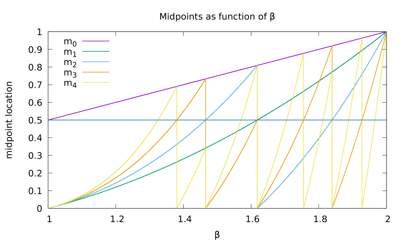
Figure 11: Location of Midpoints

This chart illustrates the location of the first five midpoints, $m_{0},m_{1},\cdots,m_{4}$ as a function of $\beta$. When $m_{k}=0.5$, further iteration is ambiguous, as this is the location of the discontinuity in the shift map, and the next iteration leaves the midpoint bifurcated. These are the “trouble spots”. The first trouble spot is visible for $m_{1}=1/2$, corresponding to $\beta=\varphi$ and a length of $\nu=2$. The midpoint $m_{2}$ crosses $1/2$ (in the ascending direction) at $\beta=1.465\cdots$ and $\beta=1.839\cdots$, corresponding to orbits of length $\nu=3$. It also crosses discontinuously downwards at $\beta=\varphi$. This crossing point has already been assigned to a shorter orbit. The midpoint $m_{3}$ has three new crossings. It also rises to touch $1/2$ at $\beta=\varphi$; but this has already been assigned to shorter orbits. The midpoint $m_{4}$ has six new crossings. Crossings will generally fall to the left and right of earlier crossings, and so are related in a bracketing relationship. The bracketing is not the full binary tree; it is pruned, as shorter orbit assignments can knock out longer one. For example, $m_{4}$ falls back down at the $m_{2}$ crossing at $\beta=1.465\cdots$, and so, here, $m_{4}$ never even gets close to $1/2$; it won’t bracket until later. This is a formalized version of figure 3, which shows midpoints of all orders.