Hierarchical Clustering for Euclidean Data

Abstract

Recent works on Hierarchical Clustering (HC), a well-studied problem in exploratory data analysis, have focused on optimizing various objective functions for this problem under arbitrary similarity measures. In this paper we take the first step and give novel scalable algorithms for this problem tailored to Euclidean data in $\mathbb{R}^{d}$ and under vector-based similarity measures, a prevalent model in several typical machine learning applications. We focus primarily on the popular Gaussian kernel and other related measures, presenting our results through the lens of the objective introduced recently by Moseley and Wang (2017). We show that the approximation factor in Moseley and Wang (2017) can be improved for Euclidean data. We further demonstrate both theoretically and experimentally that our algorithms scale to very high dimension $d$, while outperforming average-linkage and showing competitive results against other less scalable approaches.

1 Introduction

Hierarchical clustering is a popular data analysis method, with various applications in data mining (Berkhin, 2006), phylogeny (Eisen et al., 1998), and even finance (Tumminello et al., 2010). In practice, simple agglomerative procedures like average-linkage, single-linkage and complete-linkage are often used for this task (See the book by Manning, Raghavan, and Schütze (2008) for a comprehensive discussion). While the study of hierarchical clustering has focused on algorithms, there was a lack of objective functions to measure the quality of the output and compare the performance of algorithms. To remedy this, Dasgupta (2016) recently introduced and studied an interesting objective function for hierarchical clustering for similarity measures.

The input to the above problem is a set of points $V$ with a similarity measure $w_{ij}$ between $i$ and $j$. Given a hierarchical clustering represented by a tree $\mathcal{T}$ whose leaves correspond to points in $V$, Dasgupta’s objective is defined as $\mathcal{F}^{-}(\mathcal{T})=\sum_{(i,j)\in E}w_{ij}|\{x\in T(i,j)\}|,$ where $T(i,j)$ is the subtree of $\mathcal{T}$ rooted in the least common ancestor of $i$ and $j$ in $\mathcal{T}$. Dasgupta showed that solutions obtained from minimizing this objective has several desirable properties, which prompted a line of work on objective driven algorithms for hierarchical clustering, resulting in new algorithms as well as shedding light on the performance of classical methods (Roy and Pokutta, 2016; Charikar and Chatziafratis, 2017; Cohen-Addad et al., 2018).

Recently, this viewpoint has been applied to understand the performance of average linkage agglomerative clustering, one of the most popular algorithms used in practice. Moseley and Wang (2017) introduced a new objective, in some sense dual to the objective introduced by Dasgupta:

$$\mathcal{F}^{+}(\mathcal{T})=\sum_{(i,j)\in E}w_{ij}(|V|-|\{x\in T(i,j)\}|),$$

They showed that Average-Linkage obtains a $\frac{1}{3}$-approximation for maximizing this objective function.

It turns out that a random solution also achieves a $\frac{1}{3}$-approximation ratio for this problem. Recently Charikar, Chatziafratis, and Niazadeh (2019) showed that in the worst case, the approximation ratio achieved by Average-Linkage is no better than $\frac{1}{3}$ for maximizing $\mathcal{F}^{+}(\mathcal{T})$. They also gave an SDP based algorithm that achieves a ($\frac{1}{3}+\epsilon$)-approximation for the problem, for small constant $\epsilon$.

One drawback of the prior work on these hierarchical clustering objectives is the fact that they all consider arbitrary similarity scores (specified as an $n\times n$ matrix); however, there is much more structure to such similarity scores in practice. In this paper, we initiate the study of the commonly encountered case of Euclidean data, where the similarity score $w_{ij}$ is computed by applying a monotone decreasing function to the Euclidean distance between $i$ and $j$. Roughly speaking, we show how to exploit this structure to design improved approximation/faster algorithms for hierarchical clustering, and how to re-analyze algorithms commonly used in practice. In this paper, we focus on the problem of maximizing $\mathcal{F}^{+}(\mathcal{T})$, introduced by Moseley and Wang (2017).

Arguably the most common distance-based similarity measure used for Euclidean data is the Gaussian kernel. Here we use the spherical version $w_{ij}\sim\exp(-\|v_{i}-v_{j}\|/2\sigma^{2})$. The parameter $\sigma^{2}$, referred to as the bandwidth, plays an important role for applications and a large body of literature exists on selection of this parameter (Zelnik-Manor and Perona, 2005).

As discussed above, devising simple practical algorithms that improve on the $\frac{1}{3}$-approximation for general similarity measures appears to be a major challenge as observed in Moseley and Wang (2017); Charikar et al. (2019). In this paper, we show that this approximation can be improved for Euclidean data, through fast algorithms that can be scaled to very large datasets. While it might seem that the case of Euclidean data with the Gaussian kernel is a very restricted class of inputs to the HC problem, we show that for suitably high dimensions and suitable small choice of bandwidth $\sigma^{2}$ it can simulate arbitrary similarity scores (scaled appropriately). Thus any improvements to approximation guarantees for the Euclidean case (that do not apply to general similar scores) must necessarily involve assumptions about the dimension of the data (not very high) or on $\sigma^{2}$ (not pathologically small). Such assumptions on $\sigma^{2}$ are consistent with common methods for computing the bandwidth parameter based on data (e.g., (Zelnik-Manor and Perona, 2005)).

Contributions.

We start with the simplest case of 1-dimensional Euclidean data. Even in this seemingly simple setting, obtaining an efficient algorithm that produces an exactly optimum solution seems non-trivial, motivating the study of approximation algorithms. In Section 3 we prove that two algorithms – Random Cut (RC) and Average-Linkage (AL) – obtain $\frac{1}{2}$-approximation of the optimal solution, i.e., tree maximizing $\mathcal{F}^{+}(\mathcal{T})$ (AL achieves this deterministically, while RC only in expectation). This beats the best known approximation for the general case, which is $0.336$ (Charikar et al., 2019). Here RC is substantially faster than AL, with a running time of $O(n\log n)$ vs. $O(n^{2})$.

We next consider the high-dimensional case with the Gaussian Kernel and show that Average-Linkage cannot beat the factor $\frac{1}{3}$ even in poly-logarithmic dimensions. We propose the Projected Random Cut (PRC) algorithm that gets a constant improvement over $\frac{1}{3}$, irrespective of the dimension $d$ (the improvement is a function of the ratio of the diameter to $\sigma^{2}$, and drops as this ratio gets large).

Furthermore, PRC runs in $O(n(d+\log n))$ time while Average-Linkage runs in $O(dn^{2})$ time. Even single-linkage runs in almost-linear time only for constant $d$ and has exponential dependence on the dimension (see e.g., Yaroslavtsev and Vadapalli (2018)) and it is open whether it can be scaled to large $d$ when $n$ is large.

Experiments.

Many existing algorithms have time efficiency shortcomings, and none of them can be used for really large datasets. On the contrary, our Projected Random Cut (see Section 4) is a fast HC algorithm that scales to the largest ML datasets. The running time scales almost linearly and the algorithm can be implemented in one pass without needing to store similarities, so the memory is $O(n)$. We also evaluate its quality on a small dataset (Zoo).

Further related work.

HC has been extensively studied across different domains (we refer the reader to Berkhin (2006) for a survey). One killer application in biology is in phylogenetics Sneath and Sokal (1962); Jardine and Sibson (1968) and actually popular algorithms, like Average-Linkage are originating in this field. HC is also widely used to perform community detection in social networks (Leskovec et al., 2014; Mann et al., 2008), is used in bioinformatics (Diez et al., 2015) and even in finance (Tumminello et al., 2010). Other important applications include image and text classification (Steinbach et al., 2000b).

After a formal optimization HC objective was introduced, many works studied HC from an approximation algorithms perspective. The original top-down Sparsest Cut algorithm by Dasgupta, was later shown that it achieves an $O(\log n)$ approximation by Roy and Pokutta (2016); this was finally improved to $O(\sqrt{\log n})$ by Charikar and Chatziafratis (2017); Cohen-Addad et al. (2018). Subsequent work on beyond-worst-case analysis (Cohen-Addad et al., 2017) proposes a hierarchical stochastic block model under which an older spectral algorithm of McSherry (2001) combined with linkage steps gets a $O(1)$-approximation. Finally, alongside the objective of scaling HC to large graphs, the work of Bateni et al. (2017) presents two MapReduce implementations with a focus on minimum-spanning-tree based clusterings that scales to graphs with trillions of edges.

Open problems.

Here is a list of open questions that we remain unanswered in this paper: (1) Can one get an improvement over $\frac{1}{3}$ for the problem of maximizing $\mathcal{F}^{+}(\mathcal{T})$ as a function of $d$ for small $d$? (2) Can projection on low-dimensional subspaces be used to improve the approximation ratio for the high-dimensional case further? (3) Does Average-Linkage achieve a $3/4$-approximation for 1-dimensional data?

2 Preliminaries

Euclidean data.

We consider data sets represented as sets of $d$-dimensional feature vectors. Suppose these vectors are $v_{1},\ldots,v_{n}\in\mathbb{R}^{d}$. We focus on similarity measures between pairs of data points, denoted by $[w_{ij}]_{i,j\in[n]}$, where the similarities only depend on the underlying vectors, i.e., $w_{ij}=f(v_{i},v_{j})$ for some function $f:\mathbb{R}^{d}\times\mathbb{R}^{d}\rightarrow[0,1]$ and furthermore are fully determined by monotone functions of distances between them.

Definition 2.1 (Distance-based similarity measure).

A similarity measure $w_{ij}=f(v_{i},v_{j})$ is “distance-based” if $f(v_{i},v_{j})=g(\|v_{i}-v_{j}\|_{2})$ for some function $g\colon\mathbb{R}\to[0,1]$, and is “monotone distance-based” if furthermore $g\colon\mathbb{R}\to[0,1]$ is a monotone non-increasing function.

As an example of the monotone similarity measure it is natural to consider the Gaussian kernel similarity, i.e.,

$$w_{ij}=(\sqrt{2\pi}\sigma)^{-n}e^{-\frac{\|v_{i}-v_{j}\|_{2}^{2}}{2\sigma^{2}}},$$ (Gaussian Kernel)

where $\sigma$ is a normalization factor determining the bandwidth of the Gaussian kernel (Gärtner, 2003). For simplicity, we ignore the multiplicative factor $(\sqrt{2\pi}\sigma)^{-n}$ (unless noted otherwise), as our focus is on multiplicative approximations and scaling has no effects.

Linkage-based hierarchical clustering.

Among various algorithms popular in practice for HC, we focus on two very popular ones: single-linkage and average-linkage, which are two simple agglomerative clustering algorithms that recursively merge pairs of nodes (or super nodes) to create the final binary tree. Single-linkage picks the pair of super nodes with the maximum similarity weight between their data points, i.e., merges $A$ and $B$ maximizing $\max_{i\in A,j\in B}w_{ij}$. On the contrary, average-linkage picks the pair of super-nodes with maximum average similarity weight at each step, i.e., merges $A$ and $B$ maximizing $\frac{w_{AB}}{\lvert A\rvert\cdot\lvert B\rvert}$, where $w_{AB}:=\sum_{i\in A,j\in B}w_{ij}$. Average-linkage has an approximation ratio of $1/3$ for maximizing the $\mathcal{F}^{+}$ objective function (Moseley and Wang, 2017), and this factor is tight (Charikar et al., 2019).

General upper bounds.

In order to analyze the linkage-based clustering algorithms and our proposed algorithms, we propose a natural upper bound on the value of the $\mathcal{F}^{+}$ objective function. The idea is to decompose the objective function $\mathcal{F}^{+}$ into contributions of triple of vertices:

$$\mathcal{F}^{+}(\mathcal{T})=\sum_{i<j<k}\left(w_{ij}\mathbbm{1}\left[\mathcal{E}^{k}_{ij}\right]+w_{jk}\mathbbm{1}\left[\mathcal{E}^{i}_{jk}\right]+w_{ik}\mathbbm{1}\left[\mathcal{E}^{j}_{ik}\right]\right)$$

where $\mathcal{E}^{x}_{yz}$ denotes the event that $x$ is separated first among the vertices of triple $\{x,y,z\}$ in tree $\mathcal{T}$. Note that the final tree scores only one of the similarity weights between the triple $\{i,j,k\}$. Given this observation, we define the following benchmark:

$$\texttt{MAX-upper}\triangleq\sum_{i<j<k}\max(w_{ij},w_{jk},w_{ik}),$$

Clearly, for all trees $\mathcal{T}$, $\mathcal{F}^{+}(\mathcal{T})\leq\texttt{MAX-upper}$.

One-dimensional benchmarks.

Consider the special case of 1D data points (with any monotone distance-based similarity measure as in Definition 2.1), and suppose $v_{1}\leq v_{2}\leq\ldots\leq v_{n}\in\mathbb{R}$. Now, for any triple $i<j<k$, as a simple observation we have $w_{ik}\leq\min(w_{ij},w_{jk})$. Hence we can modify the above benchmark to obtain two refined new benchmarks:

$$\texttt{1D-MAX-upper}\triangleq\sum_{i<j<k}\max(w_{ij},w_{jk}),$$

$$\texttt{1D-SUM-upper}\triangleq\sum_{i<j<k}\left(w_{ij}+w_{jk}\right).$$

Again, clearly for all trees $\mathcal{T}$ we have:

$$\mathcal{F}^{+}(\mathcal{T})\leq\texttt{1D-MAX-upper}\leq\texttt{1D-SUM-upper}$$

3 Hierarchical Clustering in 1D

In this section we look at the extreme case where the feature vectors have $d=1$, and we try to analyze the popular/natural algorithms existing in this domain by evaluating how well they approximate the objective function $\mathcal{F}^{+}$. We focus on average-linkage and Random Cut (will be formally defined later). In particular, Random Cut is a building block of our algorithm for high-dimensional data given in Section 4.

We show (1) average-linkage gives a $1/2$-approximation, and can obtain no better than $3/4$ fraction of the optimal objective value in the worst-case. We then show (2) Random Cut also is a $1/2$-approximation (in expectation) and this factor is tight. In the Appendix A, we discuss other simple algorithms: single-linkage and greedy cutting (will be defined formally later). We start by the observation that greedy cutting and single-linkage output the same tree (and so are equivalent). We finish by showing (3) there is an instance where single-linkage attains only $\frac{1}{2}$ of the optimum objective value. We further show on this instance both average-linkage and random cutting are almost optimal.

For the rest of this section, suppose we have 1D points $x_{1}\leq\ldots,\leq x_{n}\in\mathbb{R}$, where $w_{ij}=g(\lVert x_{i}-x_{j}\rVert)$ for some monotone non-increasing function $g:\mathbb{R}\rightarrow[0,1]$.

Average-linkage.

In order to simplify the notation, we define $w_{AB}$ to be $\sum_{i\in A,j\in B}w_{ij}$ for any two sets $A$ and $B$. We first prove a simple structural property of average-linkage in 1D.

Lemma 3.1.

For $d=1$, under any monotone distance-based similarity measure $w_{ij}=g(\lVert x_{i}-x_{j}\rVert)$, average-linkage can always merge neighbouring clusters.

Proof.

We do the proof by induction. This property holds at the first step of average-linkage (base of induction). Now suppose up to a particular step of average-linkage, the algorithm has always merged neighbours. At this step, we have an ordered collection of super nodes $(C_{1},\ldots,C_{m})$, where for every $i<j$ and for all $(x,y)\in C_{i}\times C_{j}$, $x\leq y$. If at this step average-linkage doesn’t merge two neighbouring super nodes, then there exists $i<j<k$, where

$$\frac{w_{C_{i}C_{j}}}{\lvert C_{i}\rvert\lvert C_{j}\rvert}<\frac{w_{C_{i}C_{k}}}{\lvert C_{i}\rvert\lvert C_{k}\rvert}\Rightarrow\frac{\sum_{x\in C_{i}}w_{xC_{j}}}{\lvert C_{j}\rvert}<\frac{\sum_{x\in C_{i}}w_{xC_{k}}}{\lvert C_{k}\rvert}$$

But note that because of the monotone non-increasing distance-based similarity weights, for any triple $(x,y,z)\in C_{i}\times C_{j}\times C_{k}$ we have $w_{xy}\geq w_{xz}$, This is a contradiction to the above inequality, which finishes the inductive step. ∎

Theorem 3.2.

For $d=1$, under any monotone distance-based similarity measure $w_{ij}=g(\lVert x_{i}-x_{j}\rVert)$, average-linkage obtains at least $\tfrac{1}{2}$ of the 1D-SUM-upper, and hence is a $\frac{1}{2}$-approximation for the objective $\mathcal{F}^{+}$.

Proof.

The proof uses a potential function argument. Given a partitioning of points $x_{1}\leq x_{2}\leq\ldots\leq x_{n}$ into sets $S_{1},\ldots,S_{m}$, a triple of points $i<j<k$ is called separated if no pair of these three points belong to the same set. Now, the potential function $\Phi$ gets $\{S_{1},\ldots,S_{m}\}$ as input, and maps it to a summation over all separated triples by $\{S_{i}\}_{i\in[m]}$ as below:

$$\Phi(S_{1},\ldots,S_{m})=\sum_{i<j<k:~{}\textrm{$(i,j,k)$ is separated}}{\left(w_{ij}+w_{jk}\right)}$$

Note that $\Phi(\{x_{1}\},\ldots,\{x_{n}\})=\texttt{1D-SUM-upper}$, and $\Phi(\{x_{1},\ldots,x_{n}\})=0$.

We now run average-linkage. Based on the definition of $\mathcal{F}^{+}$, every time that average-linkage merges two super nodes $A$ and $B$ it scores $w_{AB}\cdot(n-\lvert A\rvert-\lvert B\rvert)$, and sum over of all these per-step scores is equal to its final objective value. Let Score-AL denotes the variable that stores of the score of average-linkage over time. At every step we keep track of (1) the change in the potential function, denoted by $\Delta\Phi$ and (2) how much progress average-linkage had towards the final objective value, denoted by $\Delta\texttt{Score-AL}$. In order to prove $1/2$-approximation, it suffices to show that at every step of average-linkage we have:

$$\Delta\texttt{Score-AL}+\frac{1}{2}\Delta\Phi\geq 0. \star$$ ()

To see this note that average-linkage starts with all points separated, and ends with one cluster/super node with all the points. Therefore, by summing eq. $\star$ over all merging steps of average-linkage and canceling the terms in the telescopic sum, we have:

$$(\mathcal{F}^{+}(\mathcal{T}_{\textrm{AL}})-0)+$$

$$\frac{1}{2}\left(\Phi(\{x_{1},\ldots,x_{n}\})-\Phi(\{x_{1}\},\ldots,\{x_{n}\})\right)\geq 0.$$

Plugging values of $\Phi$ at the start and the end, we get:

$$\mathcal{F}^{+}(\mathcal{T}_{\textrm{AL}})\geq\frac{1}{2}(\texttt{1D-SUM-upper}),$$

which implies the $1/2$-approximation factor.

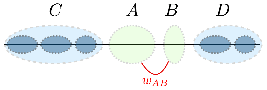
To prove eq. $\star$, we focus on a single step of average-linkage where by Lemma 3.1 some two neighboring clusters denoted as $A$ and $B$ get merged. Let $C$ denote the nodes on the left of $A$ and let $D$ denote the nodes on the right of $B$ (Figure 1). By merging two clusters $A,B$, the change in the score of average-linkage is:

$$\Delta\texttt{Score-AL}=w_{AB}(\lvert C\rvert+\lvert D\rvert)$$

Moreover, any separated triple $i<j<k$ such that either $i\in C,j\in A,k\in B$ or $i\in A,j\in B,k\in D$ will not be separated anymore after this merge. For each such triple, the potential function drops by $w_{ij}+w_{jk}$. Therefore:

$$-\Delta\Phi=\left(w_{AB}|C|+w_{AC}|B|\right)+\left(w_{AB}|D|+w_{BD}|A|\right)$$

To compare the two, we show that $w_{AB}(|C|+|D|)\geq w_{AC}|B|+w_{BD}|A|$, and hence:

$$\Delta\texttt{Score-AL} =w_{AB}(|C|+|D|)\geq w_{AC}|B|+w_{BD}|A|$$

$$=-\Delta\Phi-\Delta\texttt{Score-AL}~{},$$

which implies eq. $\star$ as desired. To prove the last claim, note that average-linkage picks the pair $(A,B)$ over both $(A,C)$ and $(B,D)$. Therefore, by definition of average-linkage:

$$\dfrac{w_{AB}}{|A||B|}\geq\dfrac{w_{AC}}{|A||C|}\implies w_{AB}|C|\geq w_{AC}|B|$$

$$\dfrac{w_{AB}}{|A||B|}\geq\dfrac{w_{BD}}{|B||D|}\implies w_{AB}|D|\geq w_{BD}|A|$$

By summing above inequalities, we get $w_{AB}(|C|+|D|)\geq w_{AC}|B|+w_{BD}|A|$, which finishes the proof. ∎

Figure 1: Illustration of the merging process in 1D.

As a final note, in Section 5 we discuss hard instances for average-linkage under Gaussian kernels when $d=1$, where we essentially show the result of Theorem 3.2 is tight when comparing against 1D-SUM-upper, and there is no hope to get an approximation factor better than $\frac{3}{4}$ for average-linkage in general for $d=1$.

Random Cut.

The following algorithm (termed as Random Cut) picks a uniformly random point $r$ in the range $[x_{1},x_{n}]$ and divides the set of points into left and right using $r$ as the splitter. The same process is applied recursively until the leaves are reached.

Algorithm 1 Random Cut

  Input: Integer $n$, points $x_{1}\leq\dots\leq x_{n}$. 

  Output: Binary tree with leaves $(x_{1},\dots,x_{n})$ 

   

  if $n==1$ then

     return  New leaf containing $x_{1}$.

  end if

  Pick $r\sim U([x_{1},x_{n}])$  

  Let $m$ be the largest integer such that $x_{m}\leq r$.  

  Create new internal tree node $x$.  

  $x.left=\textsc{Random Cut}(m,x_{1},\dots,x_{m})$ 

  $x.right=\textsc{Random Cut}(n-m,x_{m+1},\dots,x_{n})$ 

  return  $x$

Lemma 3.3.

For $d=1$ under any monotone distance-based similarity measure $w_{ij}=g(x_{i},x_{j})$ the algorithm Random Cut obtains at least $1/2$ fraction of the 1D-MAX-upper, and hence gives a $\frac{1}{2}$-approximation for the objective $\mathcal{F}^{+}$ in expectation.

Proof.

For every triple $i<j<k$ conditioned on partitioning the interval $[i,k]$ for the first time the longer edge amongst $(x_{i},x_{j})$ and $(x_{j},x_{k})$ gets cut with probability $p_{1}\geq 1/2$ and the shorter with probability $p_{2}\leq 1/2$ so that $p_{1}+p_{2}=1$. W.l.o.g let’s assume that $(x_{i},x_{j})$ is the longer edge. Then the algorithm Random Cut scores $w_{jk}p_{1}+w_{ij}(1-p_{1})$ in expectation for the $(i,j,k)$ triple. Note that:

$$w_{jk}p_{1}+w_{ij}(1-p_{1})=(w_{jk}-w_{ij})\left(p_{1}-\frac{1}{2}\right)+\frac{1}{2}(w_{ij}+w_{jk})\geq\frac{1}{2}(w_{ij}+w_{jk})$$

By the linearity of expectation taking the sum over all triples $i<j<k$ Random Cut scores at least $1/2$ of 1D-MAX-upper in expectation and hence gives $\frac{1}{2}$-approximation for the objective $\mathcal{F}^{+}$. ∎

4 Hierarchical Clustering in High Dimensions

We now describe an algorithm Projected Random Cut which we use for high-dimensional data. This algorithm is given as Algorithm 2. It first projects on a random spherical Gaussian vector and then clusters the resulting projections using Random Cut.

Algorithm 2 Projected Random Cut

  Input: Integer $n$, vectors $v_{1},\dots,v_{n}\in\mathbb{R}^{d}$. 

  Output: Binary tree with leaves $(v_{1},\dots,v_{n})$ 

   

  Pick a random Gaussian vector $\mathbf{g}\sim N_{d}(0,1)$ 

  Compute dot products $x_{i}=\langle v_{i},\mathbf{g}\rangle$  

  $x_{i_{1}},\dots x_{i_{n}}=\textsc{Sort}(x_{1},\dots,x_{n})$  

  return  $\textsc{Random Cut}(n,x_{i_{1}},\dots,x_{i_{n}})$ 

Theorem 4.1.

For any input set of vectors $v_{1},\dots,v_{n}\in\mathbb{R}^{d}$ the algorithm Projected Random Cut gives an $\alpha$-approximation (in expectation) for the objective $\mathcal{F}^{+}$ under the Gaussian kernel similarity measure $w_{ij}\sim e^{-\|v_{i}-v_{j}\|_{2}^{2}/2\sigma^{2}}$ where $\alpha=(1+\delta)/3$ for $\delta=\min_{i,j}\exp(-\frac{\|v_{i}-v_{j}\|_{2}^{2}}{2\sigma^{2}})$.

Proof.

Recall an upper bound on the optimum:

$$OPT\leq\texttt{MAX-upper}=\sum_{i<j<k}\max(w_{ij},w_{ik},w_{jk}).$$

Fix any triple $(i,j,k)$ where $i<j<k$. Note that the objective value achieved by the algorithm Projected Random Cut can also be expressed as $ALG=\sum_{i<j<k}ALG_{i,j,k}$ where $ALG_{i,j,k}$ is the contribution to the objective from the triple $(i,j,k)$ defined as follows. Consider the tree constructed by the algorithm. If $v_{k}$ is the first vector in the triple $(v_{i},v_{j},v_{k})$ to be separated from the other two in the hierarchical partition (starting from the root) then $A_{i,j,k}$ is defined to be $w_{ij}$ (in the other two cases when $i$ or $j$ are separated first the definition is analogous). Note that since Projected Random Cut is a randomized algorithm $ALG_{i,j,k}$ is a random variable. By the linearity of expectation we have $\mathbb{E}[ALG]=\sum_{i<j<k}\mathbb{E}[ALG_{i,j,k}]$. Thus in order to complete the proof it suffices to show that for every $i<j<k$ it holds that:

$$\mathbb{E}[ALG_{i,j,k}]\geq\alpha\max(w_{ij},w_{ik},w_{jk}).$$

Fix any triple $(v_{i},v_{j},v_{k})$ which forms a triangle in $\mathbb{R}^{d}$. Conditioned on cutting this triangle for the first time let $(p_{ij},p_{ik},p_{jk})$ be the vector of probabilities corresponding to the events that the corresponding edge is not cut. I.e. this is the probability that we score the contribution of this edge in the objective. Note that $p_{ij}+p_{ik}+p_{jk}=1$.

Consider any triangle whose vertices are $v_{i},v_{j},v_{k}$. To simplify presentation we set $i=1,j=2,k=3$. We can assume that $\|v_{2}-v_{1}\|\geq\|v_{2}-v_{3}\|\geq\|v_{1}-v_{3}\|$. Let $\theta_{1}=\angle\left(v_{1}-v_{3},v_{2}-v_{3}\right)$, $\theta_{2}=\angle\left(v_{2}-v_{1},v_{3}-v_{1}\right)$ and $\theta_{3}=\angle\left(v_{1}-v_{2},v_{3}-v_{2}\right)$ so that $\theta_{1}\geq\theta_{2}\geq\theta_{3}$. See Figure 2. Note that the probability that the $i$-th longest side of the triangle has the longest projection is then $\theta_{i}/\pi$.

Figure 2: Projecting the triangle $(v_{1},v_{2},v_{3})$ on $\mathbf{g}$.

Lemma 4.2.

If $(v_{1},v_{3})$ is the shortest edge in the triangle $(v_{1},v_{2},v_{3})$ then it holds that $p_{13}\geq\frac{1}{3}$

Proof.

Suppose that $\mathbf{g}$ forms an angle $\pi/2-\theta$ with $(v_{3}-v_{1})$, i.e. the vector $\mathbf{g}^{\perp}$ orthogonal to $\mathbf{g}$ forms angle $\theta$ with $v_{3}-v_{1}$. We define three auxiliary points $x,y,z$ as follows (see also Figure 2.). Let $\ell_{1}$ be a line parallel to $\mathbf{g}^{\perp}$ going through $v_{3}$, let $\ell_{2}$ to be a line parallel to $\mathbf{g}$ going through $v_{2}$ and let $\ell_{3}$ be the line parallel to $\ell_{1}$ going through $v_{1}$. We then let $x$ be the intersection of $\ell_{1}$ and $(v_{1},v_{2})$, $y$ be the intersection of $\ell_{1}$ and $\ell_{2}$ and $z$ be the intersection of $\ell_{2}$ and $\ell_{3}$ (see Fig 2).

Thus the projections of $v_{3}-v_{1}$, $v_{2}-v_{1}$ and $v_{2}-v_{3}$ on $\mathbf{g}$ are $y-z$, $v_{2}-z$ and $v_{2}-y$. Hence conditioned on $(v_{1},v_{2})$ having the longest projection the probability of scoring the contribution of $(v_{2},v_{3})$ is given as $p_{23}^{12}(\theta)=\frac{\|y-z\|}{\|y-v_{2}\|}$ since we are applying the Random Cut algorithm after the projection. Note that by Thales’s theorem we have $p_{23}^{12}(\theta)=\frac{\|y-z\|}{\|y-v_{2}\|}=\frac{\|x-v_{1}\|}{\|v_{2}-v_{1}\|}$. Applying the law of sines to the triangles $(v_{1},v_{2},v_{3})$ and $(x,v_{1},v_{3})$ we have:

$$\frac{\sin\theta_{1}}{\|v_{1}-v_{2}\|}=\frac{\sin(\theta_{1}+\theta_{2})}{\|v_{1}-v_{3}\|},\quad\frac{\sin\theta}{\|v_{1}-v_{3}\|}=\frac{\sin(\theta+\theta_{2})}{\|v_{1}-x\|},$$

where we used the fact that $\sin\theta_{3}=\sin(\pi-\theta_{1}-\theta_{2})=\sin(\theta_{1}+\theta_{2})$. Similarly, we use the fact that $\sin(\angle\left(v_{3}-x,v_{1}-x\right))=\sin(\theta+\theta_{2})$. Using the above we can express $p_{23}^{12}(\theta)$ as:

$$p_{23}^{12}(\theta)=\frac{\sin\theta}{\sin(\theta+\theta_{2})}\frac{\sin(\theta_{1}+\theta_{2})}{\sin\theta_{1}}$$

Thus the overall probability of scoring the contribution of the edge $(v_{1},v_{3})$ conditioned on $(v_{1},v_{2})$ having the longest projection which we denote as $p_{13}^{12}$ is given as:

$$p_{23}^{12} =\frac{1}{\theta_{1}}\int_{0}^{\theta_{1}}p_{23}^{12}d\theta$$

Similarly, consider the probability $p_{13}^{12}$ of scoring the contribution of $(v_{1},v_{3})$ conditioned on $(v_{1},v_{2})$ having the longest projection. We can express it as:

$$p_{13}^{12} =\frac{1}{\theta_{1}}\int_{0}^{\theta_{1}}p_{13}^{12}(\theta)d\theta,$$

where

$$p_{13}^{12}(\theta)=\frac{\sin\theta}{\sin(\theta+\theta_{3})}\frac{\sin(\theta_{1}+\theta_{3})}{\sin\theta_{1}}.$$

Below we will show that $p_{13}^{12}\geq p_{23}^{12}$. In fact, we will show that for any fixed $\theta\in[0,\theta_{1}]$ it holds that $p_{13}^{12}(\theta)\geq p_{23}^{12}(\theta)$. Comparing the expressions for both it suffices to show that $\frac{\sin(\theta_{1}+\theta_{3})}{\sin(\theta+\theta_{3})}\geq\frac{\sin(\theta_{1}+\theta_{2})}{\sin(\theta+\theta_{2})}$ for all $\theta\in[0,\theta_{1}]$. Since $\theta_{1}=\pi-\theta_{2}-\theta_{3}$ this is equivalent to:

$$\frac{\sin\theta_{3}}{\sin(\theta+\theta_{2})}\leq\frac{\sin\theta_{2}}{\sin(\theta+\theta_{3})}$$

It suffices to show that:

$$\sin\theta_{3}\sin(\theta+\theta_{3})\leq\sin\theta_{2}\sin(\theta+\theta_{2})$$

Using the formula $\sin\alpha\sin\beta=\frac{1}{2}(\cos(\alpha-\beta)-\cos(\alpha+\beta))$ it suffices to show that:

$$\cos(\theta+2\theta_{3})\geq\cos(\theta+2\theta_{2}).$$

The above inequality follows for all $\theta\in[0,\pi-\theta_{2}-\theta_{3}]$ since $\theta_{3}\leq\theta_{2}$ . This shows that $p_{13}^{12}\geq p_{23}^{12}$. Since the probability that $(v_{1},v_{2})$ has the longest projection is $\theta_{1}/\pi$ we have that the probability of scoring $(v_{1},v_{3})$ and $(v_{1},v_{2})$ having the longest projection is at least $\frac{\theta_{1}}{2\pi}$. An analogous argument shows that the probability of scoring $(v_{1},v_{3})$ and $(v_{2},v_{3})$ having the longest projection is at least $\frac{\theta_{2}}{2\pi}$.

Putting things together:

$$p_{13}\geq\frac{1}{2}\frac{\theta_{1}+\theta_{2}}{\pi}=\frac{1}{2}\frac{\pi-\theta_{3}}{\pi}\geq\frac{1}{3},$$

where we used that $\theta_{3}\leq\pi/3$ since $\theta_{3}\leq\theta_{2}\leq\theta_{1}$. ∎

We are now ready to complete the proof of Theorem 4.1. Let $\gamma=\frac{\frac{2}{3}\delta}{(1+\delta)}$ and note that $\gamma\geq\delta/3$ since $\delta\leq 1$. If $p_{13}\geq 1/3+\gamma$ then the desired guarantee follows immediately. Otherwise, if $p_{13}\leq 1/3+\gamma$ then we have:

$$\frac{\mathbb{E}[ALG_{1,2,3}]}{OPT_{1,2,3}} =\frac{p_{13}w_{13}+p_{12}w_{12}+p_{23}w_{23}}{w_{13}}$$

$$\geq\frac{1}{3}+\left(\frac{2}{3}-\gamma\right)\frac{w_{12}}{w_{13}}\geq\frac{1}{3}+\left(\frac{2}{3}-\gamma\right)\delta$$

$$=\frac{1}{3}+\frac{2}{3}\frac{\delta}{1+\delta}\geq\frac{1+\delta}{3},$$

where we used the fact that

$$\frac{w_{12}}{w_{13}}=e^{\frac{\|v_{1}-v_{3}\|_{2}^{2}-\|v_{1}-v_{2}\|_{2}^{2}}{2\sigma^{2}}}\geq e^{\frac{-\|v_{1}-v_{2}\|_{2}^{2}}{2\sigma^{2}}}\geq\delta.$$

∎

4.1 Gaussian Kernels with small $\delta$

Theorem 4.1 only provides an improved approximation guarantee for Projected Random Cut compared to the factor $1/3$ (i.e., the tight approximation guarantees of average-linkage in high dimensions; see Section 5) if $\delta$ is not too small, where $\delta=\min_{i,j}\exp(-\frac{\|v_{i}-v_{j}\|_{2}^{2}}{2\sigma^{2}})$. In particular, we get constant improvement if $\delta=\Omega(1)$. Is this a reasonable assumption? Interestingly, we answer this question in the affirmative by showing that if we have $\delta=\exp(-\tilde{\Omega}(n))$, then the Gaussian kernel can encode arbitrary similarity weights (up to scaling, which has no effects on multiplicative approximations). For simplicity, we only prove this result for $\{\epsilon,1\}$ weights here, while it can be generalized to arbitrary weights.

Theorem 4.3.

Given any undirected graph $G=(V,E)$ on $n$ nodes and $\epsilon>0$, there exist unit vectors $\{k_{v}\}_{v\in V}$ in $\mathbb{R}^{d}$ and bandwidth parameter $\sigma\in\mathbb{R}_{+}$, such that $d=O(n^{2})$, $\frac{1}{\sigma^{2}}=\Omega(n\log(1/\epsilon))$, and for some $\alpha>0$ we have:

$$\forall(u,v)\in E:e^{-\frac{\lVert k_{u}-k_{v}\rVert_{2}^{2}}{2\sigma^{2}}}=\alpha,$$

$$\forall(u,v)\notin E:e^{-\frac{\lVert k_{u}-k_{v}\rVert_{2}^{2}}{2\sigma^{2}}}=\alpha\epsilon.$$

Proof.

Our proof is constructive. Let $d=\binom{n}{2}$. Pick orthogonal vectors $\{x_{e}\}_{e\in E}$ in $\mathbb{R}^{d}$ such that $\lVert x_{e}\rVert_{2}=\frac{1}{d_{u}d_{v}}$, where $d_{u}$ is the degree of node $u$ in graph $G$. For each $v\in V$, define $y_{v}\in\mathbb{R}^{d}$ as follows:

$$y_{v}\triangleq\sum_{(u,v)\in E}(d_{u}d_{v})x_{uv}.$$

Note that $\lVert y_{v}\rVert_{2}^{2}=\sum_{(u,v)\in E}d_{u}^{2}d_{v}^{2}\frac{1}{d_{u}^{2}d_{v}^{2}}=d_{v}$ As the next step, pick a set of $n$ orthonormal vectors $\{z_{v}\}$ in the null space of $\{y_{v}\}_{v\in V}$. Finally, for each $v\in V$, define the final vector $k_{v}\in\mathbb{R}^{d}$ as follows:

$$k_{v}\triangleq\sqrt{1-\frac{d_{v}}{n}}z_{v}+\sqrt{\frac{1}{{n}}}y_{v}$$

First, note that these vectors have unit length:

$$\lVert k_{v}\rVert_{2}^{2}=1-\frac{d_{v}}{n}+\frac{\lVert y_{v}\rVert_{2}^{2}}{n}=1-\frac{d_{v}}{n}+\frac{d_{v}}{n}=1$$

Now, pick any two vertices $u$ and $v$. If $(u,v)\notin E$, then:

$$\langle k_{u},k_{v}\rangle =\langle\sqrt{1-\frac{d_{v}}{n}}z_{u}+\sqrt{\frac{1}{{n}}}y_{u},\sqrt{1-\frac{d_{v}}{n}}z_{v}+\sqrt{\frac{1}{{n}}}y_{v}\rangle$$

$$=\frac{1}{n}\langle y_{u},y_{v}\rangle=0~{},$$

where we used the fact that $\langle z_{u},z_{v}\rangle=0$ , $\langle z_{u},y_{v}\rangle=\langle z_{v},y_{u}\rangle=0$ and the fact that $\langle x_{e},x_{e^{\prime}}\rangle=0$ for every edge $e$ incident to $u$ and every edge $e^{\prime}$ incident to $v$, as $e\neq e^{\prime}$ when $(u,v)\notin E$. Similarly, when $(u,v)\in E$:

$$\langle k_{u},k_{v}\rangle=\frac{1}{n}\langle y_{u},y_{v}\rangle=\frac{1}{n}(d_{u}^{2}d_{v}^{2}\lVert x_{uv}\rVert_{2}^{2})=\frac{1}{n}$$

Now, consider a Gaussian kernel with bandwidth $\sigma=(n\log(1/\epsilon))^{-\frac{1}{2}}$ and vectors $\{k_{v}\}_{v\in V}$. Since $\|k_{u}-k_{v}\|_{2}^{2}=2(1-\langle k_{u},k_{v}\rangle)$ from the above calculations of the inner products it follows that:

$$\forall(u,v)\in E:e^{-\frac{\lVert k_{u}-k_{v}\rVert_{2}^{2}}{2\sigma^{2}}}=e^{\frac{1-1/n}{\sigma^{2}}},$$

$$\forall(u,v)\notin E:e^{-\frac{\lVert k_{u}-k_{v}\rVert_{2}^{2}}{2\sigma^{2}}}=e^{\frac{1}{\sigma^{2}}}.$$

Thus the ratio is $e^{-\frac{1}{n\sigma^{2}}}=\epsilon$, as desired. ∎

5 Hard Instances for Average-Linkage under Gaussian Kernel Similarity

High-dimensional case.

We embed the construction of Charikar et al. (2019) shown in Figure 3 into vectors with similarities given by the Gaussian kernel.

Theorem 5.1.

There exists a set of vectors $v_{1},\dots,v_{n}\in\mathbb{R}^{d}$ for $d=poly(\log n)$ for which the average-linkage clustering algorithm achieves an approximation at most $\frac{1}{3}+o(1)$ for $\mathcal{F}^{+}$ under the Gaussian kernel similarity measure.

Proof of Theorem 5.

We start by this theorem:

Theorem 5.2 (Charikar et al. (2019)).

For any constant $\epsilon\in(0,1)$ the instance $\mathcal{I}$ average-linkage clustering achieves the value of $\mathcal{F}^{+}$ at most $\frac{1}{6}n^{8/3}+O(n^{7/3})$ while the optimum is at least $\frac{1}{2}n^{8/3}-O(n^{7/3})$.

Figure 3: Hard instance $\mathcal{I}$ from Charikar et al. (2019). Vertices in orange blocks form cliques of size $n^{2/3}$ connected by edges of similarity $1-\epsilon$, vertices in blue blocks form cliques of size $n^{1/3}$ connected by edges of similarity $1$, all other pairs have similarity $0$.

Let $\Delta,\tau>0$ be real-valued parameters to be chosen later. We use indices $i$ and $j$ to index our set of vectors. For $i\in\{1,2,\dots,n^{1/3}\}$, $j\in\{1,2,\dots,n^{2/3}\}$ let

$$v_{i,j}=\Delta(e_{i}+(1+\tau)e_{k+j}),$$

where $k=n^{1/3}$ and $e_{i}$ is the $t$-th standard unit vector $e_{t}=(0\dots,1,\dots,0)$ with the $1$ in the $t$-th entry. Then it is easy to see that for any fixed $i\in[n^{1/3}]$ and $j_{1}\neq j_{2}\in[n^{2/3}]$ it holds that:

$$\|v_{i,j_{1}}-v_{i,j_{2}}\|_{2}^{2}=2(1+\tau)^{2}\Delta^{2}$$

Similarly, for any fixed $j\in[n^{2/3}]$ and $i_{1}\neq i_{2}\in[n^{1/3}]$ it holds that:

$$\|v_{i_{1},j}-v_{i_{2},j}\|_{2}^{2}=2\Delta^{2}.$$

Otherwise if $i_{1}\neq i_{2}\in[n^{1/3}]$ and $j_{1}\neq j_{2}\in[n^{2/3}]$ then:

$$\|v_{i_{1},j_{1}}-v_{i_{2},j_{2}}\|_{2}^{2}=2\Delta^{2}+2(1+\tau)^{2}\Delta^{2}\geq 4\Delta^{2}.$$

By setting $\Delta^{2}=2\sigma^{2}c\log n$ for a sufficiently large constant $c$ the contribution of pairs of vectors with $i_{1}\neq i_{2}$ and $j_{1}\neq j_{2}$ can be made negligible. Let $2(1+\tau)^{2}\Delta^{2}=\alpha$ and $2\Delta^{2}=\beta$. The rest of the pairs correspond to an hard instance $\mathcal{I}$ for which average-linkage only achieves a $\frac{1}{3}+o(1)$-approximation compared to the optimum. By setting $\tau=1/poly(\log(n))$ we have $e^{(\beta^{2}-\alpha^{2})/2\sigma^{2}}=\Omega(1)$ and hence by Theorem 5.2 it follows that average-linkage clustering can’t achieve better than $1/3+o(1)$ approximation for this instance.

Finally, note that by applying the Johnson-Lindenstrauss transform we can reduce the dimension required for the above reduction to $d=poly(\log n)$. Indeed, projecting on a random subspace of dimension $O(\frac{\log n}{\xi^{2}})$ would preserve $\ell_{2}^{2}$-distances between all pairs of vectors up to a multiplicative factor of $(1\pm\xi)$ setting $\xi=\frac{\tau}{10}=1/poly(\log n)$ it follows that our hard instance can be embedded in dimension $d=poly(\log n)$. ∎

Low-dimensional case.

For $d=1$ a hard instance for average-linkage clustering can also be constructed.

Lemma 5.3.

For points $x_{1},\dots,x_{n}\in\mathbb{R}$ average-linkage clustering achieves approximation at most $3/4$ for $\mathcal{F}^{+}$ under the Gaussian kernel similarity measure.

Proof.

Consider the instance consisting of four equally spaced points on a line, i.e. $0,\Delta,2\Delta,3\Delta$. Then (after shifting the two middle points slightly) the average-linkage clustering algorithm might first connect the two middle points and then connect the two other points in arbitrary order. We denote the cost of this solution as $AVG$. An alternative solution would be to create two groups $(0,\Delta)$ and $(2\Delta,3\Delta)$ and then merge them together. We denote the cost of this solution as $OPT$. By making $\Delta$ sufficiently large the contribution of pairs at distance more than $\Delta$ from each other can be ignored. We thus have $AVG\leq(\sqrt{2\pi}\sigma)^{-n}(3e^{-\Delta^{2}/2\sigma^{2}}+o(e^{-\Delta^{2}/2\sigma^{2}}))$ and $OPT\geq(\sqrt{2\pi}\sigma)^{-n}4e^{-\Delta^{2}/2\sigma^{2}}$, which gives the ratio of $3/4$ for sufficiently large $\Delta$. ∎

Corollary 5.4.

In the four-point instance of the proof of Lemma 5.3, the 1D-SUM-upper evaluates to
$(\sqrt{2\pi}\sigma)^{-n}6e^{-\Delta^{2}/2\sigma^{2}}$, and hence average-linkage cannot obtain more than $1/2$ of 1D-SUM-upper.

6 Experimental Results

In this section we demonstrate the quality of the solution returned by Projected Random Cut (PRC) on a small dataset, and highlight that running time only scales linearly on a large dataset. PRC does not compute the similarity weights (i.e., it only takes one pass over the feature vectors with dimension-free memory requirements) and then sorts the projected points in time $O(n\log n)$. Hence, it is fast even in use-cases with over millions of datapoints (in contrast to average-linkage, spectral clustering, or even single-linkage which all have superlinear running times in high dimensions).

We run PRC algorithm on two real datasets from the UCI ML repository (Lichman, 2013): (1) the Zoo dataset (Lichman, 2013; Vikram and Dasgupta, 2016) (the small dataset) that contains 100 animals given as 16D feature vectors (this dataset comes from applications in biology), and (2) the SIFT10M dataset (Fu et al., 2014) (the large dataset) that contains around 10M datapoints, where each datapoint is a 128D Scale Invariant Feature Transform (SIFT) vector (this dataset comes from applications in computer vision). For more details, refer to the Appendix B.

Small dataset (Zoo).

We compare PRC to (1) the recursive spectral clustering using the second eigenvector of the normalized Laplacian of the weight matrix (Spectral) (Chatziafratis et al., 2018), (2) average-linkage (AL), and (3) MAX-upper, an upper-bound on the objective value of the optimum tree; see Section 2. In contrast to PRC, these three benchmarks need to compute the weights and are slow on large datasets.

Table 1 summarizes the results of this experiment for various choices of the parameter $\sigma$ (first column). The second, third and fourth columns report the objective values (i.e., $\mathcal{F}^{+}$) of the trees returned by PRC, Spectral and AL respectively, and the fifth column gives an empirically observed approximation guarantee for PRC by comparing it against the upper bound on optimum MAX-upper. We observe that PRC attains high approximation factors of $\approx[0.73,\ldots,0.92]$ compared to MAX-upper . Moreover, PRC obtains competitive objective values compared to Spectral and AL, although it runs faster (in almost linear-time).

$\sigma$	PRC	Spectral	AL	MAX-upper	$\tfrac{\textsc{PRC}}{\texttt{MAX-upper}}$
1.5	48	61	28	64	0.75
2	64	83	47	87	0.74
2.5	83	100	66	105	0.79
3	100	112	82	117	0.85
3.5	111	121	95	126	0.87
4	117	128	105	132	0.88
4.5	123	133	114	137	0.91
5	129	137	120	140	0.92

Table 1: Values of the objective (times $10^{-3}$) on the Zoo dataset (averaged over 10 runs).

On the choice of bandwidth parameter $\sigma$, as a rule of thumb, we find an interval $[\alpha,\beta]$ such that (1) if $\sigma>\beta$, a considerable portion of pairs of datapoints with very different weights under the cosine similarities (Steinbach et al., 2000a) have almost equal weights under the Gaussian kernel, and (2) if $\sigma<\alpha$, a considerable portion of pairs of datapoints with almost equal weights under the cosine similarities have very different weights under the Gaussian kernel. We end up with $\alpha=1.5,\beta=5$.

Large dataset (SIFT10M)

The focus of this experiment is measuring the running time of PRC, and showing that it only scales linearly with the dataset size. Note that evaluating the performance of any other algorithm or upper bound (or even one pass over the similarity matrix) would be prohibitive.

We run PRC on truncated versions of SIFT10M of sizes 10K, 100K, 500K, 1M and 10M. $\sigma$ is set to 450 . We emphasize that our PRC algorithm runs extremely fast on a 2014 MacBook. The running times are summarized in Table 2. Observe that PRC scales almost linearly with the data and has almost the same running time as just a single pass over the datapoints.

Size	PRC (seconds)	1 Data Pass (seconds)
10K	1.7	1.5
100K	13	9.6
500K	67	46.4
1M	135	99.7
10M	1592	1144

Table 2: Running times of PRC and one pass.

Appendix A Greedy Cutting and Single-linkage.

Consider a simple algorithm, denoted by Greedy Cut, that picks the interval with maximum length among $\{[x_{i},x_{i}+1]\}_{i=1:n-1}$ (lets say $[x_{m},x_{m+1}]$), and repeats the same operation recursively on $(x_{1},\ldots,x_{m})$ and $(x_{m+1},\ldots,x_{n})$ until the leaves are reached.

Lemma A.1.

For $d=1$ and under any monotone distance-based similarity measure $g$ Greedy Cut and single-linkage return the same HC tree. Moreover, the edges picked by Greedy Cut are exactly the same edges picked by single-linkage, picked in reverse order.

Proof.

It is known that single-linkage is essentially the Kruskal algorithm (and hence edges picked by single-linkage form a Maximum Spanning Tree (MST)). Clearly, for any monotone distance-based measure the line connecting $x_{1}$ to $x_{n}$ is the unique MST (as any tree can be shortcut-ed with this line), and hence single-linkage picks intervals $\{[x_{i},x_{i+1}]\}_{i=1:n-1}$ in increasing order of their lengths. At the same time, Greedy Cut picks also the same intervals, but in decreasing order of their length. Moreover, because single-linkage merges the edges picked by Greedy Cut in the reverse ordering (and it creates the HC tree from bottom to top), it returns the same HC tree as Greedy Cut. ∎

Remark A.2.

As a simple observation, Greedy Cut is equivalent to reverse-Kruskal in 1D; It starts from all edges, goes over them in increasing order of weights (here, in decreasing order of lengths), and only keeps an edge when its removal makes the graph disconnected. We claim the first edge picked by reverse-kurskal corresponds to the interval $[x_{m},x_{m+1}]$ with the maximum length, and hence the equivalence between the two algorithms by induction. To prove the claim, the line between $x_{1}$ and $x_{n}$ keeps the graph connected, so the first picked edge corresponds to an interval $(x_{i},x_{i+1})$. Also, it should be the interval $[x_{m},x_{m+1}]$ with maximum length. Moreover, removing this edge makes the graph disconnected, because otherwise there is was cross edge between the left-side $(x_{1},...,x_{m})$ and the right-side $(x_{m+1},\ldots,x_{n})$. The length of such an edge is more than the length of $(x_{m},x_{m+1})$, so it should have been removed before, a contradiction.

We finish the section by demonstrating the lack of performance of single-linkage (and hence Greedy Cut) through an example, which justifies using both average-linkage and Random Cut as smooth versions of single-linkage for 1D data points.

Lemma A.3.

For $d=1$, single-linkage can obtain at most $\tfrac{1}{2}$ of the optimum objective, and $\tfrac{1}{2}$ of the objective values of average-linkage and Random Cut, under Gaussian kernels.

Proof.

Consider an example with $n$ equally spaced points on a line, where the distance between any two adjacent node is $\Delta$. We now slightly move the points so that weight of $(x_{i},x_{i+1})$ is $(\sqrt{2\pi}\sigma)^{-n}(1-(i-1)\epsilon)e^{-\Delta^{2}/2\sigma^{2}}$ for $i=1:n-1$. Now, single-linkage peels off points in the order $x_{1},\ldots,x_{n}$. Roughly speaking, we let $\Delta/\sigma^{2}$ to be large enough so we can ignore the similarity weights between any two non-adjacent points. Hence single-linkage gets an objective value of $\approx\left(\sum_{i=1}^{n-1}(n-i)\right)(\sqrt{2\pi}\sigma)^{-n}e^{-\Delta^{2}/2\sigma^{2}}$, which evaluates to $\left(n^{2}/2+o(n^{2})\right)(\sqrt{2\pi}\sigma)^{-n}e^{-\Delta^{2}/2\sigma^{2}}$. Average-linkage returns the symmetric binary tree (and hence the objective value is

$$\left((n-2)(n-1)-n\log(n)\right)(\sqrt{2\pi}\sigma)^{-n}e^{-\Delta^{2}/2\sigma^{2}}=\left(n^{2}+o(n^{2})\right)(\sqrt{2\pi}\sigma)^{-n}e^{-\Delta^{2}/2\sigma^{2}}$$

. Random returns a random binary tree, with (roughly speaking) a similar objective value of

$$\left(n^{2}+o(n^{2})\right)(\sqrt{2\pi}\sigma)^{-n}e^{-\Delta^{2}/2\sigma^{2}}$$

in expectation. The fact that optimum objective value is as large as these two quantities finishes the proof. ∎

Appendix B Deferred Discussions in Section 6

Datasets.

We use real data in our experiments. To be able to measure the performance of produced Hierarchical Clusterings, we need to compute MAX-upper, and hence we use a small dataset. To be able to show linear scaling of running time even for tens of millions of datapoints, we will use large datasets of sizes 10K to 10M.

The small dataset: The Zoo dataset contains 100 animals given as 16-dimensional vectors, forming 7 different classes (e.g., mammals, amphibians, etc.). The features contain information about the animal’s characteristics (e.g., if it has tail, hair, fins, etc.). Here, we want to showcase the quality of the solution produced by PRC; in the case of the small dataset, we can afford keeping track of two benchmarks: the performance of the widely-used Spectral algorithm and the MAX-upper.

The large dataset: In the SIFT10M dataset, each data point is a SIFT feature, extracted from Caltech-256 Griffin et al. [2007] by the open source VLFeat library Vedaldi and Fulkerson [2010]. Caltech-256 is used as a computer vision benchmark image data set, that features a total of 256 different classes with high intra-class variations for each category. Each datapoint is a 128-dimensional vector and similar to the Zoo dataset, we use this information as features to perform fast Hierarchical Clustering. Here, we want to test the scalability of our algorithm so we use successively larger datasets from the SIFT10M dataset of 10K, 100K, 500K, 1M and finally 10M datapoints by truncating the data file as necessary.

References

- Bateni et al. [2017] MohammadHossein Bateni, Soheil Behnezhad, Mahsa Derakhshan, MohammadTaghi Hajiaghayi, Raimondas Kiveris, Silvio Lattanzi, and Vahab Mirrokni. Affinity clustering: Hierarchical clustering at scale. In Advances in Neural Information Processing Systems, pages 6864–6874, 2017.
- Berkhin [2006] Pavel Berkhin. A survey of clustering data mining techniques. In Grouping multidimensional data, pages 25–71. Springer, 2006.
- Charikar and Chatziafratis [2017] Moses Charikar and Vaggos Chatziafratis. Approximate hierarchical clustering via sparsest cut and spreading metrics. In Proceedings of the Twenty-Eighth Annual ACM-SIAM Symposium on Discrete Algorithms, pages 841–854. Society for Industrial and Applied Mathematics, 2017.
- Charikar et al. [2019] Moses Charikar, Vaggos Chatziafratis, and Rad Niazadeh. Hierarchical clustering better than average-linkage. In Proceeding of the ACM-SIAM Symposium on Discrete Algorithms, 2019.
- Chatziafratis et al. [2018] Vaggos Chatziafratis, Rad Niazadeh, and Moses Charikar. Hierarchical clustering with structural constraints. In International Conference on Machine Learning, pages 773–782, 2018.
- Cohen-Addad et al. [2017] Vincent Cohen-Addad, Varun Kanade, and Frederik Mallmann-Trenn. Hierarchical clustering beyond the worst-case. In Advances in Neural Information Processing Systems, pages 6202–6210, 2017.
- Cohen-Addad et al. [2018] Vincent Cohen-Addad, Varun Kanade, Frederik Mallmann-Trenn, and Claire Mathieu. Hierarchical clustering: Objective functions and algorithms. In Proceedings of the Twenty-Ninth Annual ACM-SIAM Symposium on Discrete Algorithms, pages 378–397. SIAM, 2018.
- Dasgupta [2016] Sanjoy Dasgupta. A cost function for similarity-based hierarchical clustering. In Proceedings of the forty-eighth annual ACM symposium on Theory of Computing, pages 118–127. ACM, 2016.
- Diez et al. [2015] Ibai Diez, Paolo Bonifazi, Iñaki Escudero, Beatriz Mateos, Miguel A Muñoz, Sebastiano Stramaglia, and Jesus M Cortes. A novel brain partition highlights the modular skeleton shared by structure and function. Scientific reports, 5:10532, 2015.
- Eisen et al. [1998] Michael B Eisen, Paul T Spellman, Patrick O Brown, and David Botstein. Cluster analysis and display of genome-wide expression patterns. Proceedings of the National Academy of Sciences, 95(25):14863–14868, 1998.
- Fu et al. [2014] Xiping Fu, Brendan McCane, Steven Mills, and Michael Albert. Nokmeans: Non-orthogonal k-means hashing. In Asian Conference on Computer Vision, pages 162–177. Springer, 2014.
- Gärtner [2003] Thomas Gärtner. A survey of kernels for structured data. ACM SIGKDD Explorations Newsletter, 5(1):49–58, 2003.
- Griffin et al. [2007] Gregory Griffin, Alex Holub, and Pietro Perona. Caltech-256 object category dataset. 2007.
- Jardine and Sibson [1968] N Jardine and R Sibson. A model for taxonomy. Mathematical Biosciences, 2(3-4):465–482, 1968.
- Leskovec et al. [2014] Jure Leskovec, Anand Rajaraman, and Jeffrey David Ullman. Mining of massive datasets. Cambridge university press, 2014.
- Lichman [2013] Moshe Lichman. Uci machine learning repository, zoo dataset, 2013. URL http://archive.ics.uci.edu/ml/datasets/zoo.
- Mann et al. [2008] Charles F Mann, David W Matula, and Eli V Olinick. The use of sparsest cuts to reveal the hierarchical community structure of social networks. Social Networks, 30(3):223–234, 2008.
- Manning et al. [2008] Christopher D. Manning, Prabhakar Raghavan, and Hinrich Schütze. Introduction to information retrieval. Cambridge University Press, 2008. ISBN 978-0-521-86571-5.
- McSherry [2001] Frank McSherry. Spectral partitioning of random graphs. In focs, page 529. IEEE, 2001.
- Moseley and Wang [2017] Benjamin Moseley and Joshua Wang. Approximation bounds for hierarchical clustering: Average linkage, bisecting k-means, and local search. In Advances in Neural Information Processing Systems, pages 3097–3106, 2017.
- Roy and Pokutta [2016] Aurko Roy and Sebastian Pokutta. Hierarchical clustering via spreading metrics. In Advances in Neural Information Processing Systems, pages 2316–2324, 2016.
- Sneath and Sokal [1962] Peter HA Sneath and Robert R Sokal. Numerical taxonomy. Nature, 193(4818):855–860, 1962.
- Steinbach et al. [2000a] Michael Steinbach, George Karypis, Vipin Kumar, et al. A comparison of document clustering techniques. In KDD workshop on text mining, volume 400, pages 525–526. Boston, 2000a.
- Steinbach et al. [2000b] Michael Steinbach, George Karypis, Vipin Kumar, et al. A comparison of document clustering techniques. In KDD workshop on text mining, volume 400, pages 525–526. Boston, 2000b.
- Tumminello et al. [2010] Michele Tumminello, Fabrizio Lillo, and Rosario N Mantegna. Correlation, hierarchies, and networks in financial markets. Journal of Economic Behavior & Organization, 75(1):40–58, 2010.
- Vedaldi and Fulkerson [2010] Andrea Vedaldi and Brian Fulkerson. Vlfeat: An open and portable library of computer vision algorithms. In Proceedings of the 18th ACM international conference on Multimedia, pages 1469–1472. ACM, 2010.
- Vikram and Dasgupta [2016] Sharad Vikram and Sanjoy Dasgupta. Interactive bayesian hierarchical clustering. In International Conference on Machine Learning, pages 2081–2090, 2016.
- Yaroslavtsev and Vadapalli [2018] Grigory Yaroslavtsev and Adithya Vadapalli. Massively parallel algorithms and hardness for single-linkage clustering under distances. In Proceedings of the 35th International Conference on Machine Learning, pages 5600–5609. PMLR, 2018.
- Zelnik-Manor and Perona [2005] Lihi Zelnik-Manor and Pietro Perona. Self-tuning spectral clustering. In Advances in neural information processing systems, pages 1601–1608, 2005.