Systematics in nucleon matrix element calculations

Abstract:

The current status of calculations of simple nucleon structure observables is reviewed, with a focus on the axial charge. A major challenge is the combination of an exponentially decaying signal-to-noise ratio and the need for large source-sink separations to eliminate excited-state contributions; efforts to understand and deal with this problem are the focus of the largest section of this review. Finite-volume effects and chiral extrapolation are also briefly discussed.

1 Introduction

The structure of nucleons has been studied extensively in experiments, and nucleons also play a vital role as experimental probes. This makes the controlled study of nucleons using lattice QCD a very attractive goal. Some of the simplest matrix elements of interest include the scalar and tensor charges, which control BSM contributions to neutron beta decay, and the sigma terms, which control the sensitivity of dark matter detection to WIMPs.

In order to make a significant impact, lattice calculations of nucleon structure must become precision calculations, with full control over all systematics. The traditional test observable is the isovector axial charge $g_{A}$:

$$\left\langle p(P,s^{\prime}\middle)|\bar{u}\gamma^{\mu}\gamma_{5}d\middle|n(P,s)\right\rangle\equiv g_{A}\bar{u}_{p}(P,s^{\prime})\gamma^{\mu}\gamma_{5}u_{n}(P,s).$$ (1)

It is simple to compute, being an isovector forward matrix element, and it is measured precisely in beta decay experiments, with the latest PDG value [1] being $g_{A}=1.2724(23)$. However, calculating it accurately has been challenging: there is a long history of results being below the experimental value. Because systematic effects in $g_{A}$ are significant and it has been studied the most extensively, the axial charge will be the exclusive focus of this review. This review will also focus on recent results, particularly those presented at this conference.

This review is organized as follows. Section 2 is a brief overview of how matrix elements are computed. Excited-state effects, which are a particularly challenging source of systematic uncertainty, are discussed at length in Section 3. Finite-volume effects and dependence on the pion mass are briefly reviewed in Sections 4 and 5. Finally, a summary and outlook is given in Section 6.

2 Methodology of matrix elements

The simplest approach for computing the forward hadronic matrix element of operator $\mathcal{O}$ is to use a single interpolator $\chi$ at zero momentum. One computes two-point and three-point functions and performs a spectral decomposition,

$$\begin{aligned} C_{\text{2pt}}(t)&\equiv\left\langle\chi(t)\chi^{\dagger}(0)\right\rangle&\qquad C_{\text{3pt}}(\tau,T)&\equiv\left\langle\chi(T)\mathcal{O}(\tau)\chi^{\dagger}(0)\right\rangle\\ &=\sum_{n}|Z_{n}|^{2}e^{-E_{n}t},&&=\sum_{n,n^{\prime}}Z_{n^{\prime}}Z_{n}^{*}\langle n^{\prime}|\mathcal{O}|n\rangle e^{-E_{n}\tau}e^{-E_{n^{\prime}}(T-\tau)},\end{aligned}$$ (2)

where $Z_{n}\equiv\langle\Omega|\chi|n\rangle$ is the overlap of the interpolator onto state $n$. In the limit where all time separations $t$, $\tau$, and $T-\tau$ are large, the ground state dominates:

$$C_{\text{2pt}}(t) \to|Z_{0}|^{2}e^{-E_{0}t}\left(1+O(e^{-\Delta Et})\right),$$ (3)

$$C_{\text{3pt}}(\tau,T) \to|Z_{0}|^{2}e^{-E_{0}t}\left(\langle 0|\mathcal{O}|0\rangle+O(e^{-\Delta E\tau})+O(e^{-\Delta E(T-\tau)}+O(e^{-\Delta ET})\right),$$ (4)

where $\Delta E\equiv E_{1}-E_{0}$ is the energy gap to the first excited state.

In the ratio method, the prefactors are cancelled to obtain the ground-state matrix element:

$$R(\tau,T)\equiv\frac{C_{\text{3pt}}(\tau,T)}{C_{\text{2pt}}(T)}\to\langle 0|\mathcal{O}|0\rangle+O(e^{-\Delta E\tau})+O(e^{-\Delta E(T-\tau)})+O(e^{-\Delta ET}).$$ (5)

For forward matrix elements, the excited-state contributions are symmetric about $\tau=T/2$. They can be minimized by placing the operator at the midpoint, yielding $R(\tfrac{T}{2},T)=\langle 0|\mathcal{O}|0\rangle+O(e^{-\Delta ET/2})$.

An alternative approach is the summation method [2, 3], which involves summing over the operator insertion time $\tau$. The terms that are independent of $\tau$ grow linearly with the source-sink separation $T$ in the sum, whereas the terms that have an exponential dependence on $\tau$ produce partial sums of geometric series. The derivative of the sum yields the ground-state matrix element:

$$S(T)\equiv a\sum_{\tau}R(\tau,T),\quad\frac{d}{dT}S(T)=\langle 0|\mathcal{O}|0\rangle+O(Te^{-\Delta ET}).$$ (6)

There is some flexibility about the interval over which $\tau$ is summed. One option is to use the “interior” region where $\mathcal{O}$ is between the source and the sink, possibly excluding a fixed number of points at each end so that the sum is from $\tau_{0}$ to $T-\tau_{0}$. Another option is to sum over the whole lattice, which is the method that was first used. In two talks at the Lattice 2010 conference [4, 5], it was pointed out that contributions from excited states decay more rapidly than for the ratio-midpoint method; this revived interest in the summation method. In practice, the summation method has been found to produce a larger statistical uncertainty than the ratio method, which can negate some of its advantage; see Fig. 1.

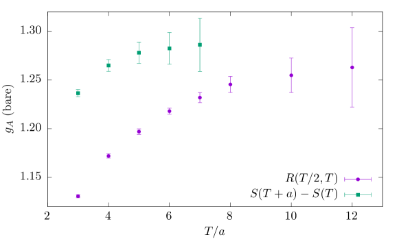
Figure 1: Bare axial charge, determined using the ratio method (purple circles) and summation method (green squares), versus source-sink separation. This calculation was performed at the physical pion mass with lattice spacing $a=0.116$ fm [6]. Note that statistics for $T/a\geq 6$ are doubled compared with $T/a<6$.

In the last few years, there has been some use of methodologies based on the Feynman-Hellmann theorem. This states that a matrix element in a given state can be obtained from the derivative of the state’s energy with respect to a perturbation in the Lagrangian:

$$\mathcal{L}(\lambda)\equiv\mathcal{L}+\lambda\mathcal{O}\implies\left.\frac{\partial}{\partial\lambda}E_{n}(\lambda)\right|_{\lambda=0}=\langle n|\mathcal{O}|n\rangle.$$ (7)

Discrete derivatives are sometimes used, particularly for the nucleon sigma terms, where the theorem relates nucleon scalar matrix elements to derivatives of the nucleon mass with respect to quark masses. Evaluating the derivative of a two-point function exactly leads directly to the summation method:

$$-\left.\frac{\partial}{\partial\lambda}\log C_{\text{2pt}}(t)\right|_{\lambda=0}=S(t),$$ (8)

where the sum is taken over all timeslices. In the large-$t$ limit, the time derivative of this equation yields Eq. (7) for the ground state. This result appeared in the original summation-method paper [2] and has been rederived in recent years [7, 8, 9].

3 Excited-state contamination

Unwanted contributions from excited states decay exponentially and will be highly suppressed if $\Delta ET\gg 1$. However, the signal-to-noise problem [10] prevents calculations from being performed at large $T$: this ratio decays as $e^{-(E_{0}-\tfrac{3}{2}m_{\pi})T}$. To be more concrete about the “brute force” approach of simply using a large source-sink separation, assume that we are using the ratio method in the asymptotic regime, where the statistical errors and excited-state contributions scale as

$$\delta_{\text{stat}}\propto N^{-1/2}e^{(m_{N}-\tfrac{3}{2}m_{\pi})T},\quad\delta_{\text{exc}}\propto e^{-\Delta ET/2},$$ (9)

respectively, where $N$ is the number of statistical samples. Supposing that we want these two uncertainties to scale together, i.e. $\delta_{\text{exc}}=\alpha\delta_{\text{stat}}\equiv\delta$ for some constant $\alpha$, then as $\delta$ is decreased the source-sink separation must be increased to suppress excited state effects. An increase in statistics is also required, both to compensate for the reduced signal-to-noise ratio, and also to meet the smaller target statistical error; the required statistics are given by

$$N\propto\delta^{-\left(2+\frac{4m_{N}-6m_{\pi}}{\Delta E}\right)}.$$ (10)

At the physical pion mass with $\Delta E=2m_{\pi}$ (see the next subsection), the exponent is roughly $-13$, much larger than the $-2$ that is obtained when neglecting excited states. This situation could be significantly improved if multilevel methods [11, 12] or other ideas [13] are able to reduce the signal-to-noise problem.

Because of the difficulty in going to large $T$, there has been much effort spent on removing excited states from data at relatively small source-sink separations: the two main approaches are improving the interpolating operator and modeling the excited-state contributions.

3.1 Theoretical expectations

An approximation to the finite-volume spectrum consists of the energy levels of any number of noninteracting stable hadrons, $E=\sum_{i,j}\sqrt{m_{i}^{2}+p_{j}^{2}}$, where $p_{j}=\tfrac{2\pi}{L}n_{j}$ and $n_{j}$ is a vector of integers. For a nucleon at rest, the leading excitations are states with a nucleon and any number of pions. Positive parity requires that for an odd number of pions there must be some nonzero momenta. These noninteracting energy gaps are shown in Fig. 2. At the physical pion mass with $m_{\pi}L=4$, the lowest excitation is $\Delta E=2m_{\pi}$ and there are eight $N\pi$ and $N\pi\pi$ levels below $4m_{\pi}$. As the box size grows, the spectrum becomes denser. On the other hand, at heavier pion masses the energies rapidly increase and there are soon just a few levels below $\Delta E=1$ GeV. Going beyond the noninteracting approximation, in Ref. [14] finite-volume quantization conditions were applied in the $N\pi$ sector using the experimentally measured scattering phase shift. Significant deviations from the noninteracting levels were found, particularly for energy gaps between 0.4 and 0.8 GeV, however the general features of the $N\pi$ spectrum were not significantly changed.

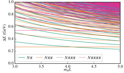
Figure 2: Energy gaps between noninteracting multiparticle excited states states and the nucleon ground state. Left: as a function of box size, at the physical pion mass. Right: versus pion mass, for $m_{\pi}L=4$. At heavier pion masses one also expects additional relatively low-lying states as resonances become stable; some possibilities include $N^{*}(1440)$, $\Delta\pi$, and $N\sigma$.

Predicting excited-state contributions to two-point and three-point functions requires knowing the spectrum $E_{n}$, the overlap factors $Z_{n}$, and the operator matrix elements $\langle n^{\prime}|\mathcal{O}|n\rangle$. The key insight that allows for study using chiral perturbation theory (ChPT) is that, if one assumes the smearing size of the interpolator is small compared with $m_{\pi}^{-1}$, then at leading order a single low-energy constant controls the coupling of a local interpolator to both nucleon and nucleon-pion states, and it is eliminated when forming ratios [15].

The prediction from ChPT for the nucleon effective mass is a percent-level excited-state contribution for $T\gtrsim 1$ fm [16, 15, 17]. On the other hand, using the ratio method, an effect at the 10% level is predicted for $g_{A}$ at $T=1$ fm [17, 18]. This effect increases the effective lattice value of $g_{A}$, in contrast with most numerical studies, which find that excited states decrease the extracted value of $g_{A}$. At this conference, O. Bär presented the first study of observables at nonzero momentum transfer, namely the form factors $G_{A}$ and $G_{P}$ of the axial current; a new tree-level diagram was found to produce a very large excited-state effect in $G_{P}$ [19].

ChPT is not expected to produce accurate results for the contributions from excited states with higher energies, particularly in the vicinity of resonances; this means that it is only expected to be valid at large source-sink separations where these contributions are suppressed, namely $T\gtrsim 2$ fm for $g_{A}$ and similar observables [20]. Deviations from ChPT for $N\pi$ states in the resonance regime were modeled in Ref. [14]; see Fig. 3. Under some model scenarios, the ratio-method result for $g_{A}$ could be suppressed by excited states at short source-sink separations and then rise to sit 1–2% above the true value for a wide range of larger source-sink separations. Clearly, this corresponds to multiple excited states contributing with different signs. This sort of scenario is particularly troublesome, as it makes systematically improving a calculation by removing excited-state effects quite difficult.

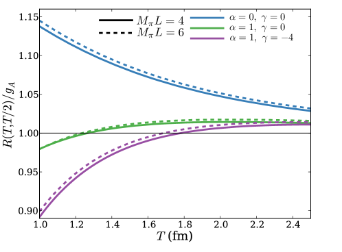
Figure 3: Model prediction of excited-state contributions to $g_{A}$ determined using the ratio method [14]. The upper pair of curves show the ChPT prediction, with the normalization of states modified using the experimental $N\pi$ phase shift and finite-volume quantization conditions. The other two pairs of curves show different scenarios for modifications to the ChPT result in the resonance regime. The figure is reproduced from Ref. [14] under the Creative Commons Attribution License.

3.2 Numerical studies

Before discussing studies in the literature, it should be noted that the available set of source-sink separations $T$ and source-operator separations $\tau$ depends on how the three-point function is computed.

• The most common approach uses a fixed sink. $C_{\text{3pt}}(\tau,T)$ is evaluated using a sequential propagator through the sink, so that $T$, the sink momentum, and the interpolating operators are fixed. All values of $\tau$ can be obtained and any quark bilinear operator $\mathcal{O}(\tau)$ can be used. The computational cost increases with every value of $T$.

• If one instead uses a fixed operator, the sequential propagator is evaluated through $\mathcal{O}(\tau)$, which is thus fixed. All values of $T$ can be obtained, and the sink momentum and interpolator can be varied. The computational cost increases with each operator insertion and with each value of $\tau$. This approach has been used recently in some variational studies by the CSSM group [21, 22].

• Rather than fixing $\tau$, one can sum over it to obtain a summed operator in the sequential propagator. In this case, $T$ becomes the only relevant time separation and all values can be obtained. The sink interpolator can be varied and the computational cost increases with each operator insertion. This approach has been used recently by CalLat [9] and NPLQCD [8].

It is possible to replace the sequential propagator with a stochastic one. This allows for increased flexibility but at the possible cost of increased noise [23, 24, 25, 26, 27].

3.2.1 Improving the nucleon interpolator

The usual proton interpolator is $\chi=\epsilon_{abc}(u^{T}_{a}C\gamma_{5}d_{b})u_{c}$, constructed using smeared quark fields. Standard practice is to tune the smearing width such that the nucleon effective mass reaches a plateau as early as possible. It is well known from spectroscopy that the variational method [28, 29], where one finds a linear combination of interpolating operators $\chi_{\text{var}}\equiv\sum_{i}c_{i}\chi_{i}$ with optimized coefficients $c_{i}$, is a powerful systematic approach for eliminating contributions from the lowest-lying excited states to estimates of energy levels and matrix elements [30, 31]. In practice, its effectiveness depends on the choice of interpolator basis $\{\chi_{i}\}$.

A simple way to produce several interpolators is to vary the smearing width; there are two recent studies that used bases comprising interpolators with three different smearing widths [33, 34]. Some results from Ref. [33] are shown in Fig. 4. The effective mass from the variationally optimized interpolator lies very close to that of the standard interpolator with the widest smearing. The optimized operator and the widest smearing also both show little sign of excited-state effects in the plateaus for the axial charge, but narrower smearings do show clear signs (see e.g. Fig. 15 of [33]). Ref. [34] also found that narrower smearings suffer from larger excited-state effects. In that study, the variationally optimized interpolator produced smaller excited-state effects than the largest smearing. However, a still larger smearing might be as good as the variational interpolator. One should take two clear lessons from these studies. The first is that tuning the smearing width is important, since it can have a significant effect on excited states. The second is that when studying a computationally more expensive alternative to the standard approach, a fair comparison should be with a well-tuned operator; it is easy to make the standard approach appear to be worse by using a too-narrow smearing.

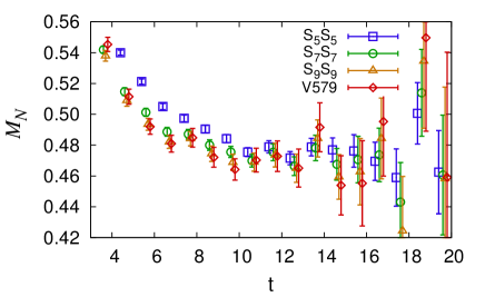
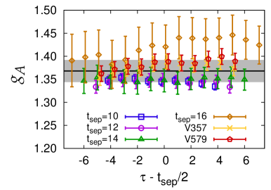
Figure 4: Comparison of analyses using a smeared standard interpolator (denoted S_i for smearing width $i$ in lattice units) and using a variationally optimized interpolator (denoted V$ijk$, using the basis $\{\text{S}_{i},\text{S}_{j},\text{S}_{k}\}$). The calculation was performed using an ensemble with $m_{\pi}=312$ MeV and $a=0.081$ fm. Left: nucleon effective mass. Right: estimators for bare $g_{A}$, using the interpolators S₉ (with four source-sink separations), V357, and V579 (with source-sink separation $12a$). The plots are reproduced from Ref. [33].

Beyond varying the smearing width, one can use different local operator structures such as $\epsilon_{abc}(u_{a}^{T}Cd_{b})\gamma_{5}u_{c}$. This approach has been used to add negative-parity interpolators to the basis, which can be important for coupling to excited states in moving frames [22]. Including covariant derivatives or the chromomagnetic field strength in the interpolator allows for a much larger basis [35, 36]. In Ref. [37], such a basis was used, employing the distillation method to efficiently construct the correlators. In general, a larger basis was more effective at removing excited-state contributions, with the largest effect seen in the tensor charge. This reference also reports that the Laplacian-Heaviside smearing used in distillation produces smaller excited-state effects from the standard operator than the more commonly used Wuppertal smearing, however it is unclear whether either smearing was tuned.

3.2.2 Fitting excited states

A natural strategy for removing contributions from excited states is to fit correlators [or derived quantities such as $R(\tau,T)$ or $S(T)$] using a model that includes excited-state effects. By far the most common model is based on a truncation of the spectral decomposition to a small number of states (two or three). Generally the two-point function provides the strongest constraints on the energies $E_{n}$ and overlaps $Z_{n}$, and the three-point function serves to determine the matrix elements $\langle n^{\prime}|\mathcal{O}|n\rangle$. Commonly, the energy gap $\Delta E$ is found to be between 0.5 and 1.0 GeV, which is usually greater than the expected lowest-lying excitation energy shown in Fig. 2.

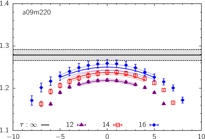
$(\tau-T/2)/a$

Figure 5: Excited-state fits for bare $g_{A}$. Both calculations were performed using the same HISQ ensemble with $a\approx 0.09$ fm and $m_{\pi}\approx 220$ MeV. Left: two-state fit to data using domain wall valence quarks and the summed operator method, with smeared and point sinks (filled circles and open squares, respectively). Right: three-state fit to data with clover valence quarks and the fixed sink method, for three source-sink separations. The left plot is adapted from Ref. [38] and the right plot is reproduced from Ref. [39] under the Creative Commons Attribution License.

Some recent examples are given in Refs. [38, 39]. In Ref. [38], the extracted value of $g_{A}$ was shown to be stable when the fit range is varied; similarly, in Ref. [39] stability was shown with respect to varying fit ranges and the number of states in the fit model. Figure 5 shows the preferred fits for $g_{A}$ on the same ensemble (albeit with different valence quark action). In both cases, the fits start with a minimum time separation of $3a$. Given the pion mass and box size, there are more than ten noninteracting excited energy levels with energy gap $\Delta E<1$ GeV; for the first points included in the fit these are only suppressed by $e^{-3a\Delta E}>0.25$. Clearly, it is difficult to associate the “excited state” in the fit with a single actual state.

At this conference, K. Ottnad presented a different fitting approach [40] that does not determine the energy gap $\Delta E$ from the two-point function. Instead, fits are performed to the ratios $R(\tau,T)$; fitting six different observables simultaneously is sufficient to constrain $\Delta E$. Interestingly, in this case the fitted energy gap approaches the expected lowest-lying noninteracting level as the minimum time separation included in the fit, $t_{\text{start}}$, is increased.

In order for these fits to be trustworthy, ideally they would be required to have good fit qualities ($p$-values). (This is not a sufficient condition!) A strong test is given in Ref. [41]: when the fit is repeated on many ensembles, the distribution of fit qualities should be uniform, which can be checked using a Kolmogorov-Smirnov (KS) test. More than half of the fit qualities in Ref. [38] are below 0.2, and hence the KS test indicates that they are not compatible with the uniform distribution ($p<10^{-3}$). In contrast, the fits in Ref. [39] are acceptable from this point of view ($p=0.26$). Some caution may be required, however, when fitting to many variables, as the difficulty in inverting a large covariance matrix can make it difficult to reliably estimate $\chi^{2}$ and the fit quality.

3.3 Outlook on excited states

It is natural to ask why the picture in Fig. 2 of low-lying $N\pi$ and $N\pi\pi$ states does not appear in the spectrum of typical variational analyses or multi-state fits. One argument is that the coupling of a multiparticle state to a local interpolator is suppressed by the inverse lattice volume. However, this should be compensated by the density of states so that in infinite volume the interpolator will couple to continua of multiparticle states. In fact, model predictions such as Fig. 3 show a weak volume dependence; this suggests that continuum spectral functions might yield suitable fit models for excited states in large volumes.

The absence of multiparticle states is familiar from meson spectroscopy. It has been found that a variational basis must include nonlocal operators in order to identify the complete and correct spectrum; see, e.g., [42]. Even though nucleon structure only requires removing excited states and not obtaining precise knowledge of them, it may still be necessary to include nonlocal operators in order to benefit in practice from the proven improved asymptotic approach to the ground state when using the variational method [30, 31].

Given that state of the art nucleon structure calculations have not reconciled their data with theoretical expectations for excited-state effects, perhaps the safest approach is to analyze data in multiple ways: ratio and summation methods, which don’t make specific assumptions about the spectrum of excitations, as well as fits that can make use of shorter time separations. This was done in the extensive excited-state study of Ref. [34], which also included a variational setup, as well as in some recent physical-pion-mass calculations by ETMC (see e.g. [43]).

4 Finite-volume effects

There is a long history of attributing a low value for $g_{A}$ computed on the lattice to finite-volume effects. These effects were computed in ChPT in Ref. [44]; neglecting loops with $\Delta$ baryons, the leading contribution at large volume is

$$\frac{g_{A}(L)-g_{A}}{g_{A}}\sim\frac{m_{\pi}^{2}g_{A}^{2}}{\pi^{2}F_{\pi}^{2}}\sqrt{\frac{\pi}{2m_{\pi}L}}e^{-m_{\pi}L}.$$ (11)

In addition to being exponentially suppressed at large $m_{\pi}L$, if one fixes $m_{\pi}L$ and decreases $m_{\pi}$ this effect will also be reduced. If this expression holds true, then a calculation with $m_{\pi}L=3$ at the physical pion mass will have smaller finite-volume effects than one with $m_{\pi}L=4$ at $m_{\pi}=300$ MeV.

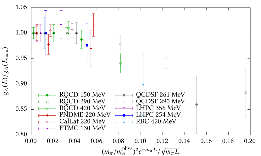
Figure 6: Controlled studies of finite-volume effects in $g_{A}$ [45, 39, 38, 46, 47, 48, 49, 50]. Each study has two or more volumes at the same pion mass, which is indicated in the legend. The largest volume of each study is used for normalization, and a black dot is placed over the symbol to indicate that the central value is fixed at one. The horizontal axis contains the dependence on pion mass and volume from Eq. (11).

There have been several fully-controlled studies of finite-volume effects in $g_{A}$, i.e., the same calculation performed on ensembles that differ only by their volume. These are summarized in Fig. 6. For large values of $m_{\pi}L$ and small pion masses, no effect is observed within uncertainties at the few percent level. As the right hand side of Eq. (11) is increased, the first significant effect is at the 5% level in the calculation by RQCD at $m_{\pi}=290$ MeV and $m_{\pi}L=3.4$. However, this is a negative effect rather than the positive effect predicted by Eq. (11). Encouragingly, the physical pion mass with $m_{\pi}L=3$ corresponds to 0.03 on the horizontal axis, where no effect has been detected.

Global fits to a set of ensembles — where the pion mass, lattice spacing, and volume are all varied — provide a different approach to study finite-volume effects. The challenge is that any failure of the fit function to accurately describe the dependence on the other variables is a source of systematic uncertainty in the estimate of finite-volume effects. This is especially true because most sets of ensembles will tend to have larger values of $m_{\pi}L$ at larger pion masses and on coarser lattice spacings. Using a global fit, Ref. [39] assumed the volume dependence of $g_{A}$ has the form $cm_{\pi}^{2}e^{-m_{\pi}L}$ with $c$ a free parameter, and found a $-0.9(5)\%$ effect at the physical pion mass with $m_{\pi}L=4$. A similar approach was used by Ref. [40], and a similar effect size was found. Finally, Ref. [38] assumed the leading heavy baryon ChPT expression and allowed a higher-order term proportional to $m_{\pi}^{3}$; this also produced a small effect at the physical pion mass.

5 Chiral extrapolation

In heavy baryon ChPT, the pion mass dependence of the axial charge is known to take the form

$$g_{A}(m_{\pi})=g_{0}-(g_{0}+2g_{0}^{3})\left(\frac{m_{\pi}}{4\pi F_{\pi}}\right)^{2}\log\frac{m_{\pi}^{2}}{\mu^{2}}+c_{1}m_{\pi}^{2}+c_{2}m_{\pi}^{3}+O(m_{\pi}^{4}),$$ (12)

where $g_{0}$ is the axial charge in the chiral limit and $c_{1,2}$ are additional low-energy constants. Although the prefactor of the chiral log is known, it is unclear how high of a pion mass can be reached before the convergence of ChPT breaks down. As a result, recent calculations that performed a chiral fit [51, 52, 38, 53, 39, 40], including results presented by R. Gupta and K. Ottnad at this conference, generally preferred to use a simple polynomial dependence on $m_{\pi}^{2}$.

The issue of chiral extrapolation can, of course, be avoided by using only lattice ensembles with near-physical pion masses. Results using this approach were presented at this conference by M. Constantinou [54], Y. Kuramashi [55], C. Lauer [46], Y. Lin [56], and S. Ohta [57].

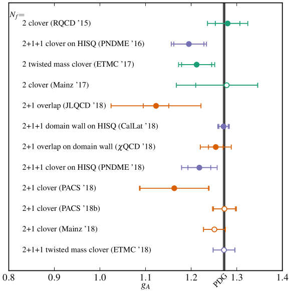
Figure 7: Recent calculations of the nucleon axial charge using $2$ flavours of dynamical sea quarks [45, 43, 51] (green), $2+1$ flavours [52, 53, 58, 55, 40] (orange), and $2+1+1$ flavours [59, 38, 39, 54] (blue). Published results are shown with a filled symbol. The PDG value [1] is indicated by the vertical band.

Figure 7 shows some recent determinations of the axial charge. It is encouraging that several collaborations are now able to reproduce the experimental value, although there is still a tendency for results to sit below experiment and no result is even half a standard deviation above experiment. Given that the experimental value is known, it may be useful for future calculations to perform a blinded analysis.

6 Summary and outlook

Excited-state contamination remains a major focus of nucleon structure calculations. A full variational study including nonlocal interpolators that couple well to multiparticle states could help to determine whether current methods are adequate. In contrast, no sign of large finite-volume effect in $g_{A}$ has been observed in the existing fully-controlled studies at low pion masses.

Discretization effects were not discussed in this review, in part because they are not universal. In general they appear to be less important than excited states, but they are nevertheless important for controlling uncertainties and can have a significant impact on the outcome such as in Ref. [39].

It should be stressed that the results in Fig. 7 have not been filtered based on any quality criteria. Such an evaluation is necessary for obtaining a reliable “lattice QCD average” of any observable. However, it may be particularly difficult to set standards for controlling excited-state effects, since analysis strategies vary significantly. A first community attempt was made in Ref. [60], and some nucleon structure will also be included in the next FLAG review.

Bringing simple observables like $g_{A}$ under precise control over all sources of systematic uncertainty will be an important step toward reliable calculations of more complex observables such as the proton charge radius and parton distribution functions. Systematics in these observables will require further study; in particular, finite-volume effects could be important for form factors [55] and discretization effects might be significant for parton distribution functions, which are generally not $O(a)$ improved.

- [1] Particle Data Group Collaboration, M. Tanabashi et al., “Review of Particle Physics,” Phys. Rev. D 98 (2018) 030001.
- [2] L. Maiani, G. Martinelli, M. L. Paciello, and B. Taglienti, “Scalar densities and baryon mass differences in lattice QCD with Wilson fermions,” Nucl. Phys. B 293 (1987) 420.
- [3] S. Güsken, U. Löw, K.-H. Mütter, R. Sommer, A. Patel, and K. Schilling, “Nonsinglet axial vector couplings of the baryon octet in lattice QCD,” Phys. Lett. B 227 (1989) 266–269.
- [4] S. Capitani, B. Knippschild, M. Della Morte, and H. Wittig, “Systematic errors in extracting nucleon properties from lattice QCD,” \posPoS(LATTICE 2010)147, 1011.1358.
- [5] ALPHA Collaboration, J. Bulava, M. A. Donnellan, and R. Sommer, “The coupling in the static limit,” \posPoS(LATTICE 2010)303, 1011.4393.
- [6] N. Hasan, J. Green, et al., “Nucleon axial, scalar and tensor charges using lattice QCD at the physical pion mass,” (in preparation) .
- [7] QCDSF/UKQCD and CSSM Collaboration, A. J. Chambers et al., “Feynman-Hellmann approach to the spin structure of hadrons,” Phys. Rev. D 90 (2014) 014510, 1405.3019.
- [8] NPLQCD Collaboration, M. J. Savage, P. E. Shanahan, B. C. Tiburzi, M. L. Wagman, F. Winter, S. R. Beane, E. Chang, Z. Davoudi, W. Detmold, and K. Orginos, “Proton-proton fusion and tritium decay from lattice quantum chromodynamics,” Phys. Rev. Lett. 119 (2017) 062002, 1610.04545.
- [9] C. Bouchard, C. C. Chang, T. Kurth, K. Orginos, and A. Walker-Loud, “On the Feynman-Hellmann theorem in quantum field theory and the calculation of matrix elements,” Phys. Rev. D 96 (2017) 014504, 1612.06963.
- [10] G. P. Lepage, “The analysis of algorithms for lattice field theory,” in From Actions to Answers: Proceedings of the 1989 Theoretical Advanced Study Institute in Elementary Particle Physics, T. DeGrand and D. Toussaint, eds., pp. 97–120. World Scientific, 1989.
- [11] M. Cè, L. Giusti, and S. Schaefer, “Domain decomposition, multi-level integration and exponential noise reduction in lattice QCD,” Phys. Rev. D 93 (2016) 094507, 1601.04587.
- [12] M. Cè, L. Giusti, and S. Schaefer, “A local factorization of the fermion determinant in lattice QCD,” Phys. Rev. D 95 (2017) 034503, 1609.02419.
- [13] W. Detmold, G. Kanwar, and M. L. Wagman, “Phase unwrapping and one-dimensional sign problems,” Phys. Rev. D 98 (2018) 074511, 1806.01832.
- [14] M. T. Hansen and H. B. Meyer, “On the effect of excited states in lattice calculations of the nucleon axial charge,” Nucl. Phys. B 923 (2017) 558–587, 1610.03843.
- [15] O. Bär, “Nucleon-pion-state contribution to nucleon two-point correlation functions,” Phys. Rev. D 92 (2015) 074504, 1503.03649.
- [16] B. C. Tiburzi, “Time dependence of nucleon correlation functions in chiral perturbation theory,” Phys. Rev. D 80 (2009) 014002, 0901.0657.
- [17] B. C. Tiburzi, “Chiral corrections to nucleon two- and three-point correlation functions,” Phys. Rev. D 91 (2015) 094510, 1503.06329.
- [18] O. Bär, “Nucleon-pion-state contribution in lattice calculations of the nucleon charges and ,” Phys. Rev. D 94 (2016) 054505, 1606.09385.
- [19] O. Bär, “Nucleon-pion-state contamination in lattice calculations of the axial form factors of the nucleon,” \posPoS(LATTICE2018)061, 1808.08738.
- [20] O. Bär, “Chiral perturbation theory and nucleon–pion-state contaminations in lattice QCD,” Int. J. Mod. Phys. A 32 (2017) 1730011, 1705.02806.
- [21] B. J. Owen, J. Dragos, W. Kamleh, D. B. Leinweber, M. S. Mahbub, B. J. Menadue, and J. M. Zanotti, “Variational approach to the calculation of ,” Phys. Lett. B 723 (2013) 217–223, 1212.4668.
- [22] F. M. Stokes, W. Kamleh, and D. B. Leinweber, “Opposite-parity contaminations in lattice nucleon form factors,” 1809.11002.
- [23] ETM Collaboration, C. Alexandrou, S. Dinter, V. Drach, K. Jansen, K. Hadjiyiannakou, and D. B. Renner, “A stochastic method for computing hadronic matrix elements,” Eur. Phys. J. C 74 (2014) 2692, 1302.2608.
- [24] G. S. Bali, S. Collins, B. Gläßle, M. Göckeler, J. Najjar, R. Rödl, A. Schäfer, A. Sternbeck, and W. Söldner, “Nucleon structure from stochastic estimators,” \posPoS(LATTICE 2013)271, 1311.1718.
- [25] Y.-B. Yang, A. Alexandru, T. Draper, M. Gong, and K.-F. Liu, “Stochastic method with low mode substitution for nucleon isovector matrix elements,” Phys. Rev. D 93 (2016) 034503, 1509.04616.
- [26] G. S. Bali, S. Collins, B. Gläßle, S. Heybrock, P. Korcyl, M. Löffler, R. Rödl, and A. Schäfer, “Baryonic and mesonic 3-point functions with open spin indices,” EPJ Web Conf. 175 (2018) 06014, 1711.02384.
- [27] A. Gambhir, “Stochastic Feynman-Hellmann,” \posPoS(LATTICE2018)126.
- [28] C. Michael, “Adjoint Sources in Lattice Gauge Theory,” Nucl. Phys. B 259 (1985) 58–76.
- [29] M. Lüscher and U. Wolff, “How to calculate the elastic scattering matrix in two-dimensional quantum field theories by numerical simulation,” Nucl. Phys. B 339 (1990) 222–252.
- [30] B. Blossier, M. Della Morte, G. von Hippel, T. Mendes, and R. Sommer, “On the generalized eigenvalue method for energies and matrix elements in lattice field theory,” JHEP 04 (2009) 094, 0902.1265.
- [31] J. Bulava, M. Donnellan, and R. Sommer, “On the computation of hadron-to-hadron transition matrix elements in lattice QCD,” JHEP 01 (2012) 140, 1108.3774.
- [32] G. Engel, C. Gattringer, L. Ya. Glozman, C. B. Lang, M. Limmer, D. Mohler, and A. Schäfer, “Baryon axial charges from Chirally Improved fermions: First results,” \posPoS(LAT2009)135, 0910.4190.
- [33] B. Yoon et al., “Controlling excited-state contamination in nucleon matrix elements,” Phys. Rev. D 93 (2016) 114506, 1602.07737.
- [34] J. Dragos, R. Horsley, W. Kamleh, D. B. Leinweber, Y. Nakamura, P. E. L. Rakow, G. Schierholz, R. D. Young, and J. M. Zanotti, “Nucleon matrix elements using the variational method in lattice QCD,” Phys. Rev. D D94 (2016) 074505, 1606.03195.
- [35] R. G. Edwards, J. J. Dudek, D. G. Richards, and S. J. Wallace, “Excited state baryon spectroscopy from lattice QCD,” Phys. Rev. D 84 (2011) 074508, 1104.5152.
- [36] J. J. Dudek and R. G. Edwards, “Hybrid baryons in QCD,” Phys. Rev. D 85 (2012) 054016, 1201.2349.
- [37] C. Egerer, D. Richards, and F. Winter, “Controlling excited-state contributions with distillation in lattice QCD calculations of nucleon isovector charges , , ,” 1810.09991.
- [38] C. C. Chang et al., “A per-cent-level determination of the nucleon axial coupling from quantum chromodynamics,” Nature 558 (2018) 91–94, 1805.12130.
- [39] R. Gupta, Y.-C. Jang, B. Yoon, H.-W. Lin, V. Cirigliano, and T. Bhattacharya, “Isovector charges of the nucleon from -flavor lattice QCD,” Phys. Rev. D 98 (2018) 034503, 1806.09006.
- [40] K. Ottnad, T. Harris, H. Meyer, G. von Hippel, J. Wilhelm, and H. Wittig, “Nucleon charges and quark momentum fraction with Wilson fermions,” \posPoS(LATTICE2018)129, 1809.10638.
- [41] Sz. Borsanyi et al., “Ab initio calculation of the neutron-proton mass difference,” Science 347 (2015) 1452–1455, 1406.4088.
- [42] D. J. Wilson, R. A. Briceño, J. J. Dudek, R. G. Edwards, and C. E. Thomas, “Coupled scattering in -wave and the resonance from lattice QCD,” Phys. Rev. D 92 (2015) 094502, 1507.02599.
- [43] C. Alexandrou, M. Constantinou, K. Hadjiyiannakou, K. Jansen, C. Kallidonis, G. Koutsou, and A. Vaquero Aviles-Casco, “Nucleon axial form factors using twisted mass fermions with a physical value of the pion mass,” Phys. Rev. D 96 (2017) 054507, 1705.03399.
- [44] S. R. Beane and M. J. Savage, “Baryon axial charge in a finite volume,” Phys. Rev. D 70 (2004) 074029, hep-ph/0404131.
- [45] RQCD Collaboration, G. S. Bali, S. Collins, B. Gläßle, M. Göckeler, J. Najjar, R. H. Rödl, A. Schäfer, R. W. Schiel, W. Söldner, and A. Sternbeck, “Nucleon isovector couplings from lattice QCD,” Phys. Rev. D 91 (2015) 054501, 1412.7336.
- [46] C. Lauer, C. Alexandrou, S. Bacchio, M. Constantinou, D. Horwarth, K. Hadjiyiannakou, G. Koutsou, and K. Jansen, “Investigating volume effects for twisted clover fermions at the physical point,” \posPoS(LATTICE2018)314.
- [47] R. Horsley, Y. Nakamura, A. Nobile, P. E. L. Rakow, G. Schierholz, and J. M. Zanotti, “Nucleon axial charge and pion decay constant from two-flavor lattice QCD,” Phys. Lett. B 732 (2014) 41–48, 1302.2233.
- [48] LHPC Collaboration, J. D. Bratt et al., “Nucleon structure from mixed action calculations using 2+1 flavors of asqtad sea and domain wall valence fermions,” Phys. Rev. D 82 (2010) 094502, 1001.3620.
- [49] J. Green, M. Engelhardt, S. Krieg, S. Meinel, J. Negele, A. Pochinsky, and S. Syritsyn, “Nucleon form factors with light Wilson quarks,” \posPoS(LATTICE 2013)276, 1310.7043.
- [50] RBC+UKQCD Collaboration, T. Yamazaki, Y. Aoki, T. Blum, H. W. Lin, M. F. Lin, S. Ohta, S. Sasaki, R. J. Tweedie, and J. M. Zanotti, “Nucleon axial charge in 2+1 flavor dynamical lattice QCD with domain wall fermions,” Phys. Rev. Lett. 100 (2008) 171602, 0801.4016.
- [51] S. Capitani, M. Della Morte, D. Djukanovic, G. M. von Hippel, J. Hua, B. Jäger, P. M. Junnarkar, H. B. Meyer, T. D. Rae, and H. Wittig, “Iso-vector axial form factors of the nucleon in two-flavour lattice QCD,” 1705.06186.
- [52] JLQCD Collaboration, N. Yamanaka, S. Hashimoto, T. Kaneko, and H. Ohki, “Nucleon charges with dynamical overlap fermions,” Phys. Rev. D 98 (2018) 054516, 1805.10507.
- [53] J. Liang, Y.-B. Yang, T. Draper, M. Gong, and K.-F. Liu, “Quark spins and anomalous Ward identity,” Phys. Rev. D 98 (2018) 074505, 1806.08366.
- [54] M. Constantinou, C. Alexandrou, S. Bacchio, K. Hadjiyiannakou, G. Koutsou, K. Jansen, and A. Vaquero, “Nucleon form factors from twisted mass fermions at the physical point,” \posPoS(LATTICE2018)142.
- [55] E. Shintani, K.-I. Ishikawa, Y. Kuramashi, S. Sasaki, and T. Yamazaki, “Nucleon form factors and root-mean-square radii on a fm lattice at the physical point,” 1811.07292.
- [56] Y. Lin, “Nucleon physics with all HISQ fermions,” \posPoS(LATTICE2018)122.
- [57] LHP, RBC, UKQCD Collaboration, S. Ohta, “Nucleon isovector axial charge in -flavor domain-wall QCD with physical mass,” \posPoS(LATTICE2018)128, 1810.09737.
- [58] PACS Collaboration, K.-I. Ishikawa, Y. Kuramashi, S. Sasaki, N. Tsukamoto, A. Ukawa, and T. Yamazaki, “Nucleon form factors on a large volume lattice near the physical point in 2+1 flavor QCD,” Phys. Rev. D 98 (2018) 074510, 1807.03974.
- [59] T. Bhattacharya, V. Cirigliano, S. Cohen, R. Gupta, H.-W. Lin, and B. Yoon, “Axial, scalar and tensor charges of the nucleon from -flavor lattice QCD,” Phys. Rev. D 94 (2016) 054508, 1606.07049.
- [60] H.-W. Lin et al., “Parton distributions and lattice QCD calculations: a community white paper,” Prog. Part. Nucl. Phys. 100 (2018) 107–160, 1711.07916.