Deep Item-based Collaborative Filtering for Sparse Implicit Feedback

Abstract.

Recommender systems are ubiquitous in the domain of e-commerce, used to improve the user experience and to market inventory, thereby increasing revenue for the site. Techniques such as item-based collaborative filtering are used to model users’ behavioral interactions with items and make recommendations from items that have similar behavioral patterns. However, there are challenges when applying these techniques on extremely sparse and volatile datasets. On some e-commerce sites, such as eBay, the volatile inventory and minimal structured information about items make it very difficult to aggregate user interactions with an item. In this work, we describe a novel deep learning-based method to address the challenges. We propose an objective function that optimizes a similarity measure between binary implicit feedback vectors between two items. We demonstrate formally and empirically that a model trained to optimize this function estimates the log of the cosine similarity between the feedback vectors. We also propose a neural network architecture optimized on this objective. We present the results of experiments comparing the output of the neural network with traditional item-based collaborative filtering models on an implicit-feedback dataset, as well as results of experiments comparing different neural network architectures on user purchase behavior on eBay. Finally, we discuss the results of an A/B test that show marked improvement of the proposed technique over eBay’s existing collaborative filtering recommender system.

1. Introduction

Recommender systems have become an integral part of many online services, improving their users’ experience by exposing them to content they may find relevant but of which they are not yet aware. On e-commerce sites, recommender systems are utilized to help buyers quickly filter through potentially enormous inventories to allow them to easily find items they would like to purchase. These systems do so by constructing models of user behavior that are used to predict whether a user is likely to engage with an item.

Two widely used techniques for modeling user affinity for items are content-based filtering and collaborative filtering. In content-based filtering, the items to be recommended are represented by characteristic features of the entities. These may include textual features (e.g. structured tags describing the items) (Lops et al., 2011), learned image representations (McAuley et al., 2015; Jing et al., 2015), and audio signals (Dieleman, 2014). Users’ preference for characteristic features are then modeled as a user profile, and at the recommendation stage, items whose content matches a user’s profile are then surfaced to the user.

In collaborative filtering (CF) methods, recommendations are made by aggregating many users’ preferences for items, and then using the aggregated preferences to make predictions for individual users. A common method for doing so, popularized by (Linden et al., 2003; Deshpande and Karypis, 2004), is item-based collaborative filtering. In item-based CF, items are represented by vectors indicating each user’s preference for that item. These preferences might be explicit (e.g., a rating of 1-5 indicating the degree of a user’s preference), or implicit (e.g., a binary vector indicating whether a user has purchased an item or not). A similarity measure, such as cosine similarity or the Pearson correlation coefficient is used to measure the similarity of user preferences between the items. To provide the top-N recommendations for a user, the similarity measure of user preferences between items is used to find the N most similar items to those for which a given user has already expressed a preference. This results in an $N$-best list of items that a user has not yet engaged with, that have similar aggregate user preferences to those items that the user has engaged with.

While having shown superior performance to content-based methods, there can be challenges in applying collaborative filtering methods. First, they have difficulty when modeling sparse user preference data. An item must have a sufficient number of user interactions before it can be meaningfully compared with other items. For item-based CF in particular, the general assumption is that there are more users than items. The problem of sparsity can lead to the cold-start problem, where items new to the system cannot be used for recommendation. Model-based approaches to collaborative filtering (e.g. (Koren et al., 2009; Salakhutdinov and Mnih, 2008; Hu et al., 2008)) oftentimes help recommendation quality on sparse datasets by learning latent representations of items only on the existing rating, while ignoring the missing data. However, these systems still suffer from the cold-start problem, and while they are better at handling sparse data than item-based CF, there still need to be a sufficient number of ratings for an item.

While effective for e-commerce sites with fixed inventory and large user bases, the challenges suffered by item-based and model-based CF approaches can limit their applications in several recommendation settings. At some e-commerce sites, like eBay, the inventory consists of approximately one billion live listings at any given time, with 160 million active users. Much of the inventory is volatile – most items are live on site for a few weeks before they are purchased. Furthermore, over half of the live listings are single quantity, that is, they can be purchased by at most one buyer, making the implicit user preference data (i.e., clicks and purchases) extremely sparse. With millions of items listed daily, the cold start problem affects a substantial portion of the inventory.

Although most listings are single quantity, oftentimes they have content descriptions and metadata that may allow us to map listings to static entities, where the listings that map to a single static entity are deemed to be equivalent. If, for example, a listing’s seller provides a UPC or other manufacturer’s identifier, we can map the item to a unique product ID associated with the identifier. Item-based CF can then be applied on the product IDs to find products with similar user purchase patterns. While this technique is effective for the top 20% most popular purchased products on eBay, the implicit user preferences on the product ID level are still very sparse. Due to the heavy-tailed nature of the distribution of purchases, recommendation quality (as evaluated by user judgment and operational metrics) on the remaining 80% of user-purchased products is low. For the remaining listings, we can map them to other types of static entities and perform CF on them. For example, we can use sets of aspects, or key-value properties of items, to construct static entities, and assign listings to the entity corresponding to the set of aspects for that listing. While the static entities constructed in this manner are very granular, and one can have a high degree of confidence that the listings that fall within an entity are equivalent items, the resulting behavioral signal is still too sparse. The majority of entities constructed in this manner still only have one purchase for each static entity. One can reduce the granularity of the static entities, by selecting subsets of aspects or single aspects for constructing entities. While this approach causes the purchase signal to be more dense, it comes at the expense of the specificity of the static entities; not all items within a static entity are truly equivalent. Another approach is to cluster listings based on the titles, and use CF on the clusters. However, applying clustering to eBay’s data is a challenge, both because of the scale and the need to tune the granularity of the clusters appropriately for the collaborative filtering objective.

The primary challenge in all these approaches is that the mapping of listings to static entities must be constructed to optimize the recommendation quality. The technique of constructing static entities first and then performing CF on the entities makes it difficult because the construction phase is removed from the measure of recommendation quality. Constructing static entities can be very time consuming, and it is often not feasible to try all combinations of aspects or item clustering hyper-parameters and evaluate recommendation quality for each entity. Instead, in this work we propose an end-to-end method that jointly learns representations of listings and uses them to predict a similarity measure of user preferences on items. The representations, which are based on embeddings of the content features of the listings, can be thought of as mapping items to implicit entities, and estimating the user preference similarity between items based on the representations. Formally, this model takes the form of a smooth function $h:(\phi(s),\phi(r))\rightarrow\text{sim}(s,r)$ that embeds a seed item $s$ (e.g. a recently purchased item) and a recommendation candidate $r$ into a latent continuous-valued vector space based on their content features $\phi$. The function $h$ estimates a proxy for the cosine similarity between the implicit user preference vectors between representations $\phi(s)$ and $\phi(r)$.

The primary contributions of this work are:

• An objective function whose optimal value is a monotonic transformation of the cosine similarity of implicit feedback vectors of two items

• A neural network architecture that embeds items into a real-valued vector space based on their content features, and optimizes the latent vectors on the cosine similarity objective

• A quantitative evaluation of the effectiveness of the objective function and the neural network architecture

The rest of the paper is organized as follows: in Section 2 we describe our objective function, demonstrate that it optimizes the cosine similarity of implicit feedback vectors, and present a Monte Carlo method for optimizing the function; Section 3 presents our neural network architecture and some variants that allow us to learn a latent representation of items; in Section 4 we present some related work on applying neural networks for recommendation system and information retrieval tasks; in Section 5 we present empirical evaluations of our objective function and neural network architecture, including empirical evidence that the objective function in Section 2 converges to the cosine similarity; Section 6 describes some qualitative properties of the learned latent item representations; and in Section 7 we describe some open questions and on-going work.

2. Objective Function

We consider a common technique for item-based collaborative filtering (Deshpande and Karypis, 2004; Linden et al., 2003). First, a model is built that captures the similarity of implicit feedback between the entities to be recommended. Then, the model is applied to generate the top-N recommendations for an active user or for a seed item. One common method of capturing the similarity is by computing the pair-wise cosine similarity of implicit feedback vectors. Consider two items $s$ and $r$. Let $\vec{s}$ and $\vec{r}$ be vectors of dimensionality $|U|$, where $U$ is the set of users in the system. $\vec{s}$ and $\vec{r}$ are vectors of user feedback. A common way of measuring behavioral similarity is by computing the cosine similarity between these two vectors:

$$\text{sim}(\vec{s},\vec{r})=\cos(\vec{s},\vec{r})=\dfrac{\sum_{i=1}^{|U|}s_{i}\cdot r_{i}}{\sqrt{\sum_{i=1}^{|U|}s_{i}^{2}}\cdot\sqrt{\sum_{i=1}^{|U|}r_{i}^{2}}}$$

In the case where the user feedback is implicit, and the vectors $\vec{s}$ and $\vec{r}$ are represented as bit vectors, the cosine similarity is equivalent to the Ochiai coefficient:

(1) $$\cos(\vec{s},\vec{r})=\dfrac{\sum_{i}\mathds{1}_{s_{i}\wedge r_{i}}}{\sqrt{\sum_{i}s_{i}}\cdot\sqrt{\sum_{i}r_{i}}}$$

Our goal is to learn a function that can estimate the cosine similarity between the implicit feedback vectors of items, based on content properties of those items.

First, we define some of our notation. Let $\mathcal{I}$ denote the set of all items, $t\in\mathcal{I}$. Our training set consists of two sets: a set of item pair co-purchase transactions $(s_{j},r_{j})\in CP$, and a set of purchased items $t_{j}\in D$. The set $CP$ represents the set of transaction pairs $(s_{j},r_{j})$, where each pair represents an event where the same user $j$ purchased both items $s\in\mathcal{I},r\in\mathcal{I}$. Similarly, let the set $D$ represent the set of transactions $t_{j}\in D$, which is the event that a user $j$ purchased an item $t\in\mathcal{I}$. Without loss of generality, assume each user will purchase an item $t\in\mathcal{I}$, or a pair of items $(s,r)\in\mathcal{I}\times\mathcal{I}$ no more than once. We define the number of times a pair of items $(s,r)\in\mathcal{I}\times\mathcal{I}$ has been purchased by the same user as

$$n_{CP}(s,r)=\sum_{(x,y)\in CP}(\mathds{1}_{x=s\wedge y=r})$$

The total number of co-purchased pairs is then given by $|CP|=\sum_{s,r}(n_{CP}(s,r))$. Similarly, the number of times an item $t\in\mathcal{I}$ has been purchased is given by

$$n_{D}(t)=\sum_{x\in D}(\mathds{1}_{x=t})$$

and the total number of purchases $|D|$ is given by $|D|=\sum_{s}(n_{D}(s))$.

Let $h(s,r)$ be a be a parameterized function (i.e. a model) that estimates the cosine similarity of implicit feedback of items $s,r\in\mathcal{I}$. Given a training set of co-purchased item pairs and purchased items $\mathcal{T}=(CP,D)$, we define the following cost function over the training set:

(2) $$\begin{split}\ell=\sum_{(s,r)\in CP}&n_{CP}(s,r)\log\sigma(h(s,r))\\ &+\sum_{s^{\prime}\in\mathcal{I}}\sum_{r^{\prime}\in\mathcal{I}}\Big{[}\sqrt{n_{D}(s^{\prime})}\sqrt{n_{D}(r^{\prime})}\log\big{[}1-\sigma(h(s^{\prime},r^{\prime}))\big{]}\Big{]}\end{split}{}$$

where $\sigma$ is the sigmoid function

$$\sigma(x)=\dfrac{1}{1+e^{-x}}$$

Note that Equation 2 is the well-known binary cross-entropy loss applied to $\mathcal{T}$ with a particular distribution of positive and negative labels. This loss function resembles negative sampling approaches used in word2vec and in other approaches to recommendation, such as (Mikolov et al., 2013b; Covington et al., 2016a; Xu et al., 2016).

We demonstrate that the value of $h(s,r)$ that minimizes this cost function for a given pair $(s,r)$ is the log of the cosine similarity expressed in Equation 1. Assuming the capacity of the model $h$ is large enough to allow exact prediction on $(s,r)$ without deviation from the optimum, each $h(s,r)$ can assume a value independently of other $(s,r)$ pairs. Decomposing the loss and calculating it on a single pair of items $(s,r)$, we get the following function for a pair:

(3) $$\ell(s,r)=n_{CP}(s,r)\log\sigma(h(s,r))+\sqrt{n_{D}(s)}\sqrt{n_{D}(r)}\log\sigma(-h(s,r))$$

Note that for convenience, here we use the fact that $1-\sigma(x)=\sigma(-x)$. To find the value of $h(s,r)$ that optimizes Equation 3, we take the partial derivative of $\ell(s,r)$ with respect to $h(s,r)$:

$$\frac{\partial\ell(s,r)}{\partial h(s,r)}=n_{CP}(s,r)\sigma(-h(s,r))-\sqrt{n_{D}(s)}\sqrt{n_{D}(r)}\sigma(h(s,r))$$

Setting this equal to 0 and solving for $h(s,r)$, we get

$$0=n_{CP}(s,r)\sigma(-h(s,r))-\sqrt{n_{D}(s)}\sqrt{n_{D}(r)}\sigma(h(s,r))$$

$$\Rightarrow 0=n_{CP}(s,r)\frac{1}{1+e^{h(s,r)}}-\sqrt{n_{D}(s)}\sqrt{n_{D}(r)}\frac{1}{1+e^{-h(s,r)}}$$

$$\Rightarrow n_{CP}(s,r)\frac{1}{1+e^{h(s,r)}}=\sqrt{n_{D}(s)}\sqrt{n_{D}(r)}\frac{1}{1+e^{-h(s,r)}}$$

$$\Rightarrow \frac{n_{CP}(s,r)}{\sqrt{n_{D}(s)}\sqrt{n_{D}(r)}}=\frac{1+e^{h(s,r)}}{1+e^{-h(s,r)}}$$

Using the fact that $\frac{1+e^{x}}{1+e^{-x}}=e^{x}$, we find that the value of $h(s,r)$ that minimizes Equation 3 is

(4) $$h(s,r)=\log\Big{[}\frac{n_{CP}(s,r)}{\sqrt{n_{D}(s)}\sqrt{n_{D}(r)}}\Big{]}$$

This is the log of Equation 1. We will validate this result empirically in Section 5.1.

Oftentimes, the cardinality of the set $\mathcal{I}\times\mathcal{I}$ is too large to be able to explicitly enumerate. As an alternative to optimizing Equation 2, we can optimize a Monte Carlo estimate. We can define the normalization factor $\mathcal{Z}\equiv\sum_{t\in\mathcal{I}}\sqrt{n_{D}(t)}$. Let $k_{CP}$ be the number of co-purchased item pairs we sample according to the distribution $P_{CP}(s,r)=\frac{n_{CP}(s,r)}{|CP|}$. Let $k_{s}$ be the number of seed items we sample as negative examples according to the distribution $P_{D}^{\sqrt{}}(s)=\frac{\sqrt{n_{D}(s)}}{\mathcal{Z}}$, and let $k_{r}$ be the number of candidate items we sample as negative examples for each negative seed item according to the distribution $P_{D}^{\sqrt{}}(r)$. Note that we draw $s$ and $r$ independently from the distribution $P_{D}^{\sqrt{}}$. We can then define the Monte Carlo estimate of the cost function in Equation 2 as

(5) $$\begin{split}\ell_{MC}=&\mathop{\mathbb{E}}_{(s,r)\sim P_{CP}}[k_{CP}\cdot\log\sigma(h(s,r))]\\ &+\mathop{\mathbb{E}}_{s^{\prime}\sim P_{D}^{\sqrt{}}}\mathop{\mathbb{E}}_{r^{\prime}\sim P_{D}^{\sqrt{}}}[k_{s}\cdot k_{r}\cdot\log\sigma(-h(s^{\prime},r^{\prime}))]\end{split}$$

We explicitly express the expectations as follows:

$$\begin{split}\ell_{MC}=&\sum_{(s,r)\in CP}\Big{[}\frac{n_{CP}(s,r)}{|CP|}\cdot k_{CP}\cdot\log\sigma(h(s,r))\Big{]}\\ &+\sum_{s^{\prime}\in\mathcal{I}}\sum_{r^{\prime}\in\mathcal{I}}\Big{[}\frac{\sqrt{n_{D}(s^{\prime})}}{\mathcal{Z}}\cdot\frac{\sqrt{n_{D}(r^{\prime})}}{\mathcal{Z}}\cdot k_{s}\cdot k_{r}\cdot\log\sigma(-h(s^{\prime},r^{\prime}))\Big{]}\end{split}$$

Then, for a specific pair of items $(s,r)$:

(6) $$\begin{split}\ell_{MC}(s,r)=&n_{CP}(s,r)\cdot\frac{k_{CP}}{|CP|}\cdot\log\sigma(h(s,r))\\ &+\sqrt{n_{D}(s)}\cdot\sqrt{n_{D}(r)}\cdot\frac{k_{s}}{\mathcal{Z}}\cdot\frac{k_{r}}{\mathcal{Z}}\cdot\log\sigma(-h(s,r))\end{split}$$

Using the same methods we used to derive Equation 4 above, we can compute the derivative of $\ell_{MC}(s,r)$ with respect to $h(s,r)$ and solve for $h(s,r)$:

$$\begin{split}\frac{\partial\ell_{MC}(s,r)}{\partial h(s,r)}=&n_{CP}(s,r)\cdot\frac{k_{CP}}{|CP|}\cdot\sigma(-h(s,r))\\ &-\sqrt{n_{D}(s)}\cdot\sqrt{n_{D}(r)}\cdot\frac{k_{s}\cdot k_{r}}{\mathcal{Z}^{2}}\cdot\sigma(h(s,r))\end{split}$$

Solving this for $h(s,r)$ gives us

(7) $$h(s,r)=\log\Big{[}\frac{n_{CP}(s,r)}{\sqrt{n_{D}(s)}\sqrt{n_{D}(r)}}\Big{]}+\log\Big{[}\frac{k_{CP}}{k_{s}\cdot k_{r}}\Big{]}+\log\Big{[}\frac{\mathcal{Z}^{2}}{|CP|}\Big{]}$$

Equation 7 indicates that the output of the model $h(s,r)$ that optimizes the cost function in Equation 5 is the cosine similarity shifted by a constant proportional to the ratio of the sampling mixture of positive and negative examples, and the ratio of the number of co-purchases in the training set and the number of purchases. In Section 5.1, we empirically demonstrate the effects of different sampling ratios $k_{CP}/k_{s}\cdot k_{r}$.

3. Model Architectures

In this section, we describe two neural network architectures that we experiment with. These architectures define the function $h(s,r)$ whose cost function in Section 2 we optimize. The networks take two items as input, encoded as sparse feature vectors. The neural network architecture can be decomposed into three sub-networks - one that computes a representation of item $s$, one that computes a representation of item $r$, and one that makes a prediction based on the embeddings of items $s$ and $r$. We first describe the architecture of the sub-networks responsible for constructing embeddings for items $s$ and $r$, and then discuss how we combine the two embeddings to make a prediction.

3.1. Item Embedding Network

For each item $t\in\mathcal{I}$, we assume we have $k$ sets of tokens associated with item $t$. One set of tokens might be a title of an item $t$; another set might consist of aspect tokens; another might consist of category information; etc. We make no a-priori assumptions about the nature of the features in each set, other than a constraint that they are text tokens. We denote each set as $t_{k}$, and a token index $i$ in the set $t_{k}$ as $t_{ki}$. Note that each item $s,r\in\mathcal{I}$ that serve as input to $h$ might have separate sets of token features $s_{k}$, $r_{k}$.

Inspired by work on word embeddings (Mikolov et al., 2013a; Mikolov et al., 2013b), we first embed each token into a lookup table, where we define a separate lookup table for each set of tokens $t_{k}$. A pooling layer then aggregates together the embedding vectors for each token $t_{ki}$ present in an item $t$ for each set $t_{k}$, yielding an embedding for each $t_{k}$. The aggregated vectors are then concatenated together for each $t$, and fed through a non-linear activation function. We then use a feed-forward layer to combine information between the different pooled vectors $t_{k}$, and finally pass the resulting vector through a non-linear activation function. A schematic of this approach, using a mean-pooling mechanism to pool together the token embeddings, can be seen in Figure 1. Note that in this work, we use $\tanh$ as the activation function. We experimented with ReLU activations as well, but found that they gave similar performance to $\tanh$.

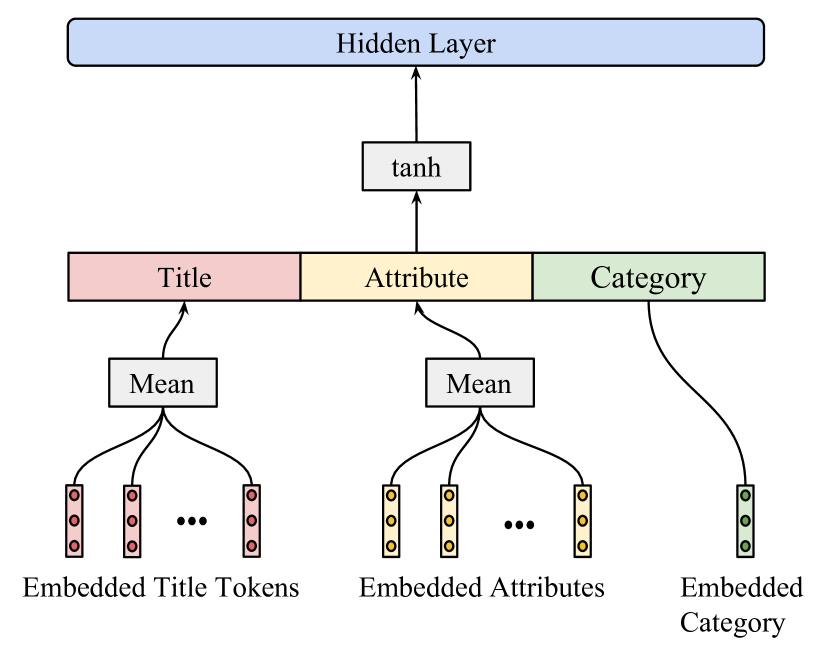
Figure 1. DCF-Mean item embedder

The choice of vector pooling mechanism can depend on the nature of the set $t_{k}$. We experiment with two methods. When we have non-sequential text features, such as tags or aspects, we apply an element-wise mean pooling layer for the vectors associated with each token $t_{ki}$. When we have sequential text features, such as titles, where the order of tokens may be relevant, we experiment with a few options – treating each sequence as a bag of words and applying element-wise mean pooling; or applying a recurrent neural network (RNN) to learn a representation of the title. We refer to the mean-pooling architecture as DCF-Mean (where DCF is an abbreviation for deep collaborative filtering), and the RNN architecture as DCF-RNN. When applying a recurrent neural network to aggregate the tokens in a text sequence, we treat the RNN as an encoder (Cho et al., 2014) and use the hidden state of the last time step as the embedding of the token sequence. The end-to-end neural network shown in Figure 2 shows the DCF-RNN variant of the item embedders. In Section 5.2, we present results on both approaches.

3.2. Prediction Network

The component of the neural network that takes the embeddings of the two items and outputs an estimate of a similarity measure is shown in Figure 2. This part of the network concatenates the latent vector representations of items $s$ and $r$, applies a fully-connected hidden layer to the concatenated vectors, applies a non-linear activation function, and finally outputs a scalar value. The dimensionality of the token embeddings, RNN hidden state, and fully-connected layers are all hyper-parameters that must be tuned. Note that the end-to-end architecture can be designed to be symmetric or asymmetric – one can tie the parameters of the two subnetworks that embed the items $s$ and $r$ so that they have the same values. Similarly, one can tie the parameters of the two halves of the matrix corresponding to the hidden layer that combines the item embeddings.

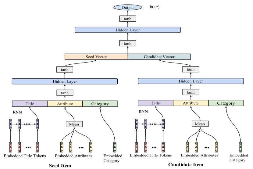
Figure 2. End-to-end neural network architecture modeling $h(s,r)$

4. Related Works

Hybrid Recommender Systems   There have been many works on incorporating content into collaborative filtering approaches. These hybrid recommender systems (refer to (Jannach et al., 2010; Burke, 2002) for a survey of the subject) use additional metadata features to augment implicit and explicit feedback signals on items. Basilico & Hofmann (Basilico and Hofmann, 2004) propose a kernel-based method that constructs feature maps of users and items, and then use perceptron learning to optimize the kernels. Melville et al. (Melville et al., 2002) propose a method that, given a sparse user-item explicit feedback matrix, first imputes the missing ratings using a content-based recommender system, and then performs collaborative filtering using this imputed matrix. Li & Kim (Li and Kim, 2003) first cluster items based on content features to create an item group matrix, and then perform collaborative filtering on the item groups, finally applying a linear combination of the results of item-based and group-based CF. Popescul et al. (Popescul et al., 2001) describe a generative probabilistic model that models a three-way co-occurrence between users, items, and item content. This model estimates the parameters of a latent variable based on the users, that the items and content are then conditioned on. Our approach is similar in spirit to these works. All these works implicitly or explicitly map items or users to representations that encode information on their content, and perform collaborative filtering on these representations. Our approach falls within this same setting, in that we learn latent representations of items based on their content features, and then condition our predictions of the distribution of co-purchases on these latent representations.

Deep Learning in Information Retrieval   In recent years, there has been a lot of attention paid to applying deep learning for different IR tasks, including recommender systems. In the context of recommender systems, several works have used deep learning to solve a variety of problems, including retweet prediction (Zhang et al., 2016), tag-aware recommendation (Xu et al., 2016; Zuo et al., 2016), personalized recommendations (Liang and Baldwin, 2015), and video recommendations (Covington et al., 2016b). Deep learning systems have also been used for IR tasks including web search (Huang et al., 2013; Jaech et al., 2017; Mitra et al., 2016) and text matching (Severyn and Moschitti, 2015; Shen et al., 2014; Hu et al., 2014; Lu and Li, 2013). Our work is most similar to (Xu et al., 2016) and (Covington et al., 2016b). Both works use a negative sampling scheme similar to (Mikolov et al., 2013a) to allow their model to scale. In our work, we also use a negative sampling scheme, but design our sampling distributions so that we converge to an estimate of the cosine similarity between implicit feedback vectors of items.

5. Experimental Studies

We designed two sets of experiments to allow us to empirically study the properties of our objective function and our neural network architectures. In the first set of experiments, we empirically validate that optimizing the cost function in Equation 2 converges to the log of the cosine distance between the implicit feedback vectors. We also study the effects of the sampling ratios when optimizing the Monte Carlo estimate in Equation 5. In our second set of experiments, discussed in Section 5.2, we compare the performance of DCF-Mean and DCF-RNN on eBay’s user behavioral data, and present the results of an A/B test comparing the new approach with eBay’s existing CF-based recommender system.

5.1. Synthetic Experiments

Synthetic Dataset   To validate that a model trained to optimize the cost function in Equation 2 optimizes the cosine similarity between implicit feedback vectors, we generated a synthetic dataset of purchases and trained a model to predict the cosine distances between the implicit vectors. We used the following procedure to generate a dataset. Let $N_{u}$ be the number of users in a system, and let $N_{i}$ be the number of items. For each item $i=1\ldots N_{i}$, we draw a random variable $p_{i}\sim\text{Uniform}(0.2,0.8)$. Then, for each user $u=1\ldots N_{u}$ and for each item $i$, we draw a random variable $r_{ui}\sim\text{Bernoulli}(p=p_{i})$ indicating whether $u$ has purchased item $i$. This gives us an implicit feedback matrix of dimensionality $N_{u}\times N_{i}$. We then construct a set of training examples from this user-item feedback matrix. For each pair of items $i,j$, we construct a feature vector of dimensionality $N_{i}\cdot N_{i}$, where all entries are set to 0 except for the entry $k=i*N_{i}+j$, which is set to 1. This has the effect of creating a feature for each pair of items $(i,j)$. For all the experiments in this section, the synthesized dataset consisted of 100 items and 10,000 users. There were 25,355,794 total co-purchases in the synthesized dataset, with a sparsity ratio of 25.35%. We experimented with several different values for the number of items, number of users and sparsity, but they made little difference in the results of the experiments described below. The only difference was in training time.

Validating Full Cost Function   To empirically validate the cost function presented in Equation 2, we trained a model on the synthetic dataset previously described. We then compared the model’s estimates of the cosine similarity between each pair of items $(i,j)$ against the true calculated cosine similarity between $i$ and $j$, using both RMSE and Spearman’s rank correlation coefficient. The training set consisted of a feature vector for each pair of items $(i,j)$, along with their co-occurrence frequencies $n_{CP}(i,j)$ and the square root of their individual frequencies $n_{D}(i)$. We trained a linear model of the following form

$$h(s,r)=\vec{\theta}x_{sr}$$

to optimize Equation 2. In this case, each parameter $\theta_{k}$ in the parameter vector will correspond to the similarity of the items $(i,j)$ (since we designed our feature vectors to be indicator variables for each pair $k=i*N_{i}+j$). We trained the model for 200 epochs with learning rate 0.1 using stochastic gradient descent. As the purpose of this experiment was to empirically validate the convergence properties, we compared the model’s output against the cosine similarity on the training set. At the conclusion of the training run, the RMSE between the calculation of the true cosine similarities on the training set and our model’s estimates was $1.0461\times 10^{-4}$, and the Spearman rank correlation coefficient was 0.9999, with $p<0.01$. Additionally, we also tracked the convergence of the model. Those results can be found in the heavy-lined curve in Figure 3.

Effect of Sampling Ratios   With very large inventories, it is often infeasible to do a full pass over all item pairs, which is a requirement for optimizing the cost function in Equation 2. As an alternative, one can use a Monte Carlo technique to approximate the expectations in the cost function in Equation 5. As demonstrated in Section 2, the value of the model output that minimizes Equation 5 is the log of the cosine similarity of the implicit feedback vectors shifted by a constant:

$$h(s,r)=\log\Big{[}\frac{n_{CP}(s,r)}{\sqrt{n_{D}(s)}\sqrt{n_{D}(r)}}\Big{]}+\log\Big{[}\frac{k_{CP}}{k_{s}\cdot k_{r}}\Big{]}+\log\Big{[}\frac{\mathcal{Z}^{2}}{|CP|}\Big{]}$$

where $k_{CP}$ is the number of true co-purchases to sample, $k_{s}$ is the number of seed items to sample, and $k_{r}$ is the number of candidate items to sample. To converge to the optimal value of Equation 2 when using Monte Carlo techniques, this result suggests that $k_{CP}$, $k_{s}$, and $k_{r}$ ought to be selected so that the ratio of samples $\frac{k_{CP}}{k_{s}\cdot k_{r}}$ is set to $\frac{|CP|}{\mathcal{Z}^{2}}$, where $|CP|$ denotes the number of co-purchased item pairs, and $\mathcal{Z}$ denotes the sum of square roots of the number of purchases of each item. Oftentimes, however, we are more interested in the ranking of similar items produced by the cosine distance rather than the values themselves. To understand the effect of the selection of $k_{CP}$, $k_{s}$, and $k_{r}$ on the convergence rate of the training algorithm, we experimented with different ratio values of $\frac{k_{CP}}{k_{s}\cdot k_{r}}$. We fixed $k_{CP}=100000$, and tried several values of $k_{s}$ and $k_{r}$, training the model for a fixed 200 epochs, where on each epoch we sampled examples from the distributions $P_{CP}$ and $P_{D}^{\sqrt{}}$. Note that for this synthetic experiment, the ratio $\frac{|CP|}{\mathcal{Z}^{2}}=0.516$. The convergence rates of different ratios are shown in Figure 3. We ran several such experiments with a variety of sparsity levels (and therefore different ratios $\frac{|CP|}{\mathcal{Z}^{2}}$), and the convergence results were comparable.

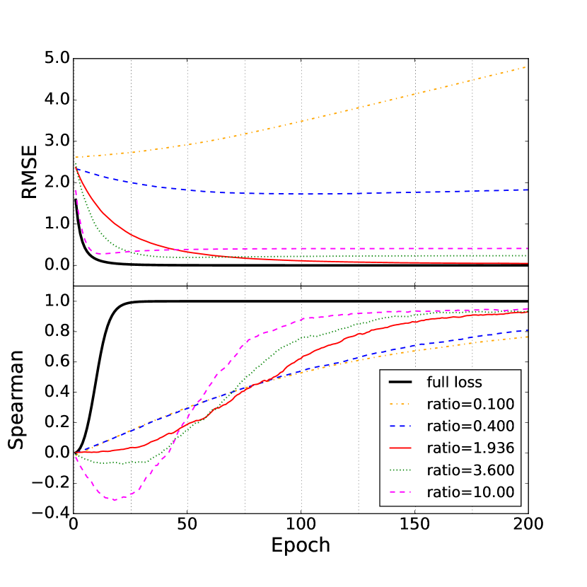
Figure 3. Effects of different ratios of $\frac{k_{CP}}{k_{s}\cdot k_{r}}$ on convergence rate of Monte Carlo loss.

As expected, setting the ratio to $\frac{|CP|}{\mathcal{Z}^{2}}$ yielded the lowest RMSE compared to the true cosine distances at convergence. The result in Section 2 indicates that setting the ratio to $\frac{|CP|}{\mathcal{Z}^{2}}$ in Equation 7 gives the optimal value in Equation 4. Interestingly, oversampling items from $P_{D}^{\sqrt{}}$ (giving a lower ratio $\frac{k_{CP}}{k_{s}\cdot k_{r}}$) caused the Spearman rank correlation coefficient between the model output and the true cosine distance to converge more quickly, although they yielded worse RMSE values. This suggests that if one is training a model for a fixed number of epochs, oversampling $k_{s}$ and $k_{r}$ would allow the model to reach a good value more quickly than setting the ratio to $\frac{|CP|}{\mathcal{Z}^{2}}$. Under-sampling $k_{s}$ and $k_{r}$, so that $\frac{k_{CP}}{k_{s}\cdot k_{r}}>\frac{|CP|}{\mathcal{Z}^{2}}$, caused the RMSE to diverge, and the Spearman Rank coefficient to converge significantly more slowly.

5.2. Experiments on eBay Data

Setting   eBay has several recommender systems in use for different recommendation settings. We concern ourselves with the setting of post-purchase recommendations, recommendations that are made after a user purchases an item (referred to as the seed item). The current post-purchase recommender system constructs a recall set of recommendation candidates for the seed item using item-based collaborative filtering on a few levels of static entities, and then applies a set of business rules to select the top N recommendations among the recall sets. Note that these results are not personalized to a user based on their entire purchase history.

Data   eBay’s inventory is segmented into a hierarchy of categories. For both our off-line experiments and for the user-facing recommender system, we trained one model for each high-level category. In this work, we present results on five of those categories: women’s fashion, electronics, skin care, outdoor sporting goods, and collectibles. These categories were selected to highlight a variety of inventory. We define the implicit feedback signals we train on as purchases – we sample pairs of listings from $P_{CP}$ that were co-purchased by the same user, and we sample purchased listings from the listing distribution $P_{D}^{\sqrt{}}$. We constructed our training sets for the five models as follows. For each of the five categories, we collected all purchases made on eBay between January 1st 2015 and May 31st 2016 under those categories. For each category, we constructed a set of co-purchased item pairs $CP$ by taking all pairs of items $(t_{1},t_{2})$ under the category purchased by the same user $u$, with the constraint that $t_{2}$ was purchased after $t_{1}$. We construct the set of purchased listings $D$ by including all purchased items under the category. Statistics about this dataset are summarized in Table 1.

Dataset	$|CP|$	$\mathcal{Z}^{2}$	# Features
Women’s Fashion	34894458	265921110	29318
Electronics	5297580	42685339	35620
Skin Care	6060626	8986127	55456
Outdoor Sporting Goods	2097230	36683099	51163
Collectibles	13904465	38635017	36169

Table 1. Statistics on training datasets for eBay

Note that this method of constructing our training set, along with the fact that we have independent parameters for the three sub-networks in Figure 2, means that our models will be asymmetric – the output of the model will not be the same if we invert the seed and candidate items.

Evaluation Methodology   To construct our test set, we sampled listings from the set of purchases made in June 2016, ensuring that the sets of test and training items were completely disjoint. From the set of June 2016 purchases, we randomly sampled 250 purchased items from each category. For each of those purchased items, we randomly sampled a subsequent purchase by the same user under the same high-level category. We refer to these 250 pairs as the set of true co-purchases. When generating recommendations on eBay, we are typically going to consider approximately 1 million recommendation candidates for each seed item. To reflect this in our evaluation setting, we require a very large recall set of candidate items, from which we will select the top 30 recommendations. Specifically, we randomly sampled 200,000 random items from the high-level category to serve as the recall set of candidates. Thus, there will be 200,001 recommendation candidates for each seed item, with one of them being a true co-purchase. The model is applied to rank this set of candidates for each seed. Because our evaluation set contains only one true co-purchased item for every seed, we evaluate our models by measuring the rank of the true co-purchased item in the list.

We evaluate our results using two measures: mean recall at $k$ and mean reciprocal rank. In information retrieval, recall at $k$ is the mean of the number of relevant results in the top $k$ of a ranked list divided by the total number of relevant results:

$$\text{rec}_{k}(s)=\frac{1}{n}\sum_{i=1}^{n}\dfrac{\#(\text{relevant results at position}>k)}{\#(\text{total number of relevant results})}$$

In our case, we have one relevant (co-purchased) item for each seed, so recall at $k$ measures the percentage of seed items for which the true co-purchase is in the top $k$ of the ranked list. On eBay, 30 recommendations are surfaced for a seed. We evaluate our models in the same setting, fixing $k=30$. To understand the performance of our model on the entire recall set and not just the top 30, we also evaluate the mean reciprocal rank of the true co-purchased item, namely:

$$\text{MRR}=\frac{1}{n}\sum_{i=1}^{n}\frac{1}{\text{rank}(i)}$$

Training Details   We demonstrated in Section 5.1 that the ideal ratio $\frac{k_{CP}}{k_{s}\cdot k_{r}}$ should be set to $\frac{|CP|}{\mathcal{Z}^{2}}$. However, the degree of sparsity in the training data makes it impractical to follow this guideline. As implied by the results in Section 5.1, and the statistics of the size of $|CP|$ and $\mathcal{Z}^{2}$ in Table 1, we would need to sample several thousand items from $P_{D}^{\sqrt{}}$ for each $s$ and $r$ for every sample from $P_{CP}$. Instead of directly optimizing Equation 5, we note that our sampling of items $s$ from $P_{D}^{\sqrt{}}$ make no difference in the ranking order of candidates for a given seed item $s$. Inspired by (Mikolov et al., 2013a; Mikolov et al., 2013b), we instead sample a fixed number of $r$ items for each seed $s$ from $P_{D}^{\sqrt{}}$. The cost function we end up optimizing for these experiments is given by:

(8) $$\begin{split}\ell=\mathop{\mathbb{E}}_{(s,r)\sim P_{CP}}\Big{[}k_{CP}\cdot\log\sigma(h(s,r))+\mathop{\mathbb{E}}_{r^{\prime}\sim P_{D}^{\sqrt{}}}[k_{r}\cdot\log\sigma(-h(s,r^{\prime}))]\Big{]}\end{split}$$

Note the similarity between this approximation and the objective function in (Mikolov et al., 2013a; Mikolov et al., 2013b).

We compare the performance of two neural network architectures for this task – one that uses mean pooling on the title token embeddings and the key-value property embeddings (DCF-Mean), shown in Figure 1, and one that uses a vanilla recurrent neural network to embed the title, while using mean pooling to aggregate the aspect embeddings (DCF-RNN), shown in Figure 2. We implemented our models and training algorithms in Theano (Theano Development Team, 2016), and trained the models on an NVIDIA Tesla M40 card, for a maximum of 1000 epochs. In practice, training time ranged between three and five days. In DCF-Mean, we fixed the token embeddings to have 200 dimensions, the hidden layer in the item embedders to have 400 dimensions, and the hidden layer in the top layer with 1200. DCF-RNN had the same setting, with the hidden state of the RNN set to 200 dimensions as well.

We compare the performance of these two neural networks against two baselines – a linear model baseline (i.e. a logistic regression model) trained to minimize Equation 8, and the current collaborative filtering method employed by eBay. The training examples for the linear model consist of binary vector representations of listings, where each item is represented by a $|V|$-dimensional vector, where $|V|$ is the size of the vocabulary for the model. If a feature is present in the listing, its corresponding entry in the feature vector is set to 1, otherwise, it is set to 0. As described in the introduction, the eBay collaborative filtering algorithm maps items to static entities and then computes the cosine similarity between implicit feedback vectors of static entities. The highest quality static entity is a product, which we derive from the UPC or other manufacturer’s identifier for an item. The fallback static entity is an aspect, of which an item may have more than one. For a given seed item $s$ and a set of candidate items $\{r_{1},\ldots,r_{k}\}$, if $s$ maps onto a product ID, then we rank the subset of $\{r_{1},\ldots,r_{k}\}$ that also map onto products by the cosine distance on purchase vectors between the products. The ranked list of products is at the top of the $N$-best list. For the remaining subset of $\{r_{1},\ldots,r_{k}\}$ that is not mapped to a product, we fetch all the aspects for each item in the list and compute the cosine similarity between all aspects of the seed and all aspects of the candidate. The score for a pair $(s,r_{i})$ is then the sum of the similarities between all property pairs. The candidates are ranked according to these scores and are appended to the list after the items mapped to products.

Quantitative Results   The results of our experiments can be found in Tables 2 and 3. We ran two sets of experiments. First, we compared the performance of different model architectures trained on the same objective function on the five categories. We compared the performance of the baseline linear model, DCF-Mean, and DCF-RNN on each of the five high-level categories. For all of these experiments, we fixed $k_{cp}=200000$ and $k_{r}=4$ for each epoch of training. We fixed the maximum number of epochs to 1000, and used early stopping on a held out validation set to stop training when the loss on the validation set stopped decreasing. The results on the test set are found in Table 2. Results in bold are statistically significant at $p<0.01$, and results in italics are statistically significant at $p<0.05$. Statistical significance was estimated using Student’s paired t-test.

Category	MRR				Recall@30
	CF Baseline	Linear	DCF-Mean	DCF-RNN	CF Baseline	Linear	DCF-Mean	DCF-RNN
Women’s Fashion	0.0063	0.001	0.018	0.024	0.016	0.016	0.104	0.100
Electronics	0.0069	0.0005	0.0055	0.002	0.020	0.004	0.040	0.024
Skin Care	0.0030	0.0001	0.0126	0.0039	0.012	0.0	0.084	0.020
Outdoor Sporting Goods	0.0058	0.0043	0.0057	0.0112	0.032	0.016	0.048	0.032
Collectibles	0.0091	0.0003	0.0112	0.0041	0.020	0.0	0.072	0.012

Table 2. Results comparing the performance of different model architectures. Results in bold indicate that the result is statistically significant over the baseline at $p<0.01$, results in italics are statistically significant at $p<0.05$.

The results indicate that with $k_{r}=4$, DCF-Mean achieves the best ranking performance over the baseline. DCF-Mean achieves statistically significant improvement over the CF-based baseline in three of the five categories. Interestingly, DCF-RNN did not achieve statistically significant improvements over the baseline, despite the fact that it is able to account for token ordering in the titles. We conjecture that our use of vanilla RNNs hampered our model’s ability to learn due to the vanishing gradient problem (we also noticed that the loss plateaued earlier for the RNN models than for DCF-Mean). In future work, we will experiment with alternative RNN formulations, such as LSTMs (Hochreiter and Schmidhuber, 1997) or GRUs (Chung et al., 2014), as well as convolutional methods (e.g., (Zhang et al., 2015)). Additionally, for two of the categories, DCF-Mean was unable to gain a statistically significant advantage over the collaborative filtering baseline. As we show below, DCF-Mean will outperform the baseline for higher values of $k_{r}$.

The second set of experiments we ran compared the effect of different selections of $k_{r}$ on the ranking performance of DCF-Mean. Generally speaking, the more items $r$ sampled from $P_{D}^{\sqrt{}}$, the larger the gain over the CF baseline. Interestingly, the strongest results were in the Women’s Fashion, Skin Care, and Collectibles categories. Purchases in these categories tend to better reflect a user’s taste (for example, collectors’ interest in certain sports memorabilia, or buyers with particular sartorial preferences) than in the more utilitarian categories of electronics or outdoor sporting goods. We conjecture that these categories are harder to learn because users’ stylistic or thematic preferences are not as often reflected in the co-purchase data. Additionally, it is important to note that the recall at $k$ and MRR measures only measure the position of the true co-purchased item in the ranked list. Given the nature of the inventory on eBay, in many settings there may be functionally equivalent items to the true co-purchased item ranked higher in the list than the true co-purchase. It is possible that given two models with equal recall at $k$ or MRR measures on the test set, one model might rank more relevant recommendations ranked above the true co-purchase than another model, but the evaluation measures do not reflect this property.

Category	MRR					Recall@30
	CF	$k_{r}=1$	$k_{r}=4$	$k_{r}=9$	$k_{r}=19$	CF	$k_{r}=1$	$k_{r}=4$	$k_{r}=9$	$k_{r}=19$
Women’s Fashion	0.0063	0.016	0.018	0.031	0.050	0.016	0.076	0.104	0.168	0.188
Electronics	0.0069	0.0018	0.0055	0.0073	0.0089	0.020	0.0	0.040	0.044	0.064
Skin Care	0.0030	0.0055	0.0126	0.0143	0.0121	0.012	0.024	0.084	0.108	0.088
Outdoor Sporting Goods	0.0058	0.0050	0.0057	0.0114	0.0125	0.032	0.032	0.048	0.084	0.076
Collectibles	0.0091	0.0053	0.0112	0.0153	0.0153	0.020	0.024	0.072	0.096	0.088

Table 3. The results comparing different number of $k_{r}$ samples. Results in bold indicate that the result is statistically significant over the baseline at $p<0.01$, results in italics are statistically significant at $p<0.05$.

A/B Test Results   As is common on e-commerce sites, we ran an A/B test comparing our approach versus the production baseline variant to evaluate the performance of the model in an on-line setting. The A/B test ran for two weeks on eBay, testing the DCF-Mean model variant against the current production variant. Table 4 lists the results, indicating an improvement of two critical metrics: click-through rate (CTR) and purchase-through rate (PTR). DCF-Mean demonstrated a 79.7% increase in CTR over the baseline and a 51.8% increase in PTR over the baseline.

	CTR	PTR
lift	+79.7%	+51.8%

Table 4. Lift in A/B test operational metrics.

6. Discussion

To understand why our method seems to work well in the setting of extreme sparsity and cold-start items, we can examine the representations the model learns for items. We conjecture that the reason the model is able to perform well is due to the semantic similarities between items with similar purchase patterns. We posit that seed items that are similar in content with each other (e.g., have similar thematic and functional semantics) are more likely to be co-purchased with candidate items that are similar in content to each other. If true, then the item representations learned by the model ought to reflect these semantics. While we currently do not have a quantitative measure of semantic similarity, we can examine a few examples of the representational similarity of items.

The listings are sorted by the distance between their vector embeddings (i.e., the hidden layer in Figure 1) from the listing whose title is in bold. For each item whose title is in bold, we computed the Euclidean distance between that item and every other item in our recall set. We then sorted the list according to distance and selected the listings at the 10th, 100th, 1000th, 10000th, 20000th, 50000th, and 100000th positions. We present the item titles in Table 5 to depict their semantic similarities.

Position	Title	Distance
0	1992 Chicago Bulls world champions drinking glasses set of 3 NBA Michael Jordan	0.0
10	1969 vintage Boston Celtics NBA championship mug stein basketball Havlicek	0.7043
100	Mickey Mantle the Mick NY Yankees August 14 1995 news tribute	0.9664
1000	Houston Texans die cut window decal by Rico industries	1.1339
10000	NFL new era New England Patriots 59Fifty Team Fitted Hat size 7 3/4’	1.2711
20000	Pittsburgh Steelers Snack Helmet by Wincraft inc. Official NFL	1.3321
50000	2015 Topps chrome WWE 45 Luke Harper wrestling card	1.505
100000	1993 Tyco vortex action figure from Double Dragon loose	1.7590
0	Virginia Tech Hokies cell phone hard case iPhone 4 & 4s	0.0
10	Boise State Broncos cell phone hard case for Apple iPhone 4 & 4s	0.3031
100	Unlimited cellular phone jelly case for Apple iPhone 4 & 4s	0.6708
1000	Blue skull crystal black finished hard case cover for Apple iPhone 6s plus, 5, 5s	0.7755
10000	Nike black hard phone case available for iPhone 6, 6s plus, 5, 5s fast shipping	0.9080
20000	New 6 plus only recover wood iPhone 6 phone cover case NIB	0.9694
50000	Magnetic gray magnetic flip wallet swede leather case for iPhone6, 6s	1.1027
100000	The adventure of case for iPhone 4,5,6, 6s and Samsung Galaxy s4, s5, s6, s7	1.2506
0	Biggs Darklighter 30th annv rebel X-Wing pilot Star Wars gold coin action figure	0.0
10	2006 Star Wars Saga collection Rogue Two snowspeeder w Zev Senesca pilot figure	0.45034447
100	2005 Hasbro Star Wars Episode iii Revenge of the Sith Chewbacca action figure	0.6689232
1000	Vintage Star Wars action figure 1980 lobot aid complete w weapon	0.9111377
10000	Star Trek V Final Frontier large action figure limited	1.0554923
20000	Harry Potter 2001 headmaster Dumbledore Sorcerers Stone action figure	1.1852574
50000	Lightcore Hex Skylanders giants new sealed ships fast	1.4289094
100000	1980’s original vintage New York Giants snapback baseball hat mint	1.669067

Table 5. Item titles sorted by the distance between their embedding representations

These examples suggest that the semantics of the items are represented in the distances between the vectors. Consider the first example in Table 5: “1992 Chicago Bulls world champions drinking glasses set of 3 NBA Michael Jordan”. The item in the tenth position is another NBA commemorative cup, one for the Boston Celtics. This is despite the fact that the only shared token between the two is the token “NBA”; the network seems to have learned to model the relationship between basketball, championships, and glasses & mugs. As one descends in the list, one gets baseball memorabilia, followed by football memorabilia, followed by a wrestling collectible card, followed by a collectible action figure. One can see similar patterns for the other items.

7. Conclusions & Future Work

In this work, we have described a machine learning objective that converges to the cosine distance between implicit feedback vectors, allowing us to train collaborative filtering models that take into account the content similarity of the items to be recommended. We have presented two neural network architectures and demonstrated that they are more effective in the context of volatile inventory and sparse behavioral implicit feedback matrices than item-based CF, in both off-line evaluation and in an on-line A/B test. There is substantial room for improvement however. Finding better methods for combining the information across token vectors, such as LSTMs or convolutional neural networks, would allow us to better model the relationships between the tokens. Additionally, we would like to extend our objective function to model the similarity in explicit feedback vectors. Finally, we believe we can improve the model performance by exploring alternative optimization methods and item sampling strategies.

References

- (1)
- Basilico and Hofmann (2004) Justin Basilico and Thomas Hofmann. 2004. Unifying Collaborative and Content-based Filtering. In Proceedings of the Twenty-first International Conference on Machine Learning (ICML ’04). ACM, New York, NY, USA, 9–.
- Burke (2002) Robin Burke. 2002. Hybrid Recommender Systems: Survey and Experiments. User Modeling and User-Adapted Interaction 12, 4 (Nov. 2002), 331–370.
- Cho et al. (2014) Kyunghyun Cho, Bart van Merrienboer, Çaglar Gülçehre, Fethi Bougares, Holger Schwenk, and Yoshua Bengio. 2014. Learning Phrase Representations using RNN Encoder-Decoder for Statistical Machine Translation. CoRR abs/1406.1078 (2014).
- Chung et al. (2014) Junyoung Chung, Çaglar Gülçehre, KyungHyun Cho, and Yoshua Bengio. 2014. Empirical Evaluation of Gated Recurrent Neural Networks on Sequence Modeling. CoRR abs/1412.3555 (2014).
- Covington et al. (2016a) Paul Covington, Jay Adams, and Emre Sargin. 2016a. Deep Neural Networks for YouTube Recommendations. In Proceedings of the 10th ACM Conference on Recommender Systems (RecSys ’16). ACM, New York, NY, USA, 191–198.
- Covington et al. (2016b) Paul Covington, Jay Adams, and Emre Sargin. 2016b. Deep Neural Networks for YouTube Recommendations. In Proceedings of the 10th ACM Conference on Recommender Systems. New York, NY, USA.
- Deshpande and Karypis (2004) Mukund Deshpande and George Karypis. 2004. Item-based top-N Recommendation Algorithms. ACM Trans. Inf. Syst. 22, 1 (Jan. 2004), 143–177.
- Dieleman (2014) Sander Dieleman. 2014. Recommending Music on Spotify with Deep Learning. http://benanne.github.io/2014/08/05/spotify-cnns.html. (2014).
- Hochreiter and Schmidhuber (1997) Sepp Hochreiter and Jürgen Schmidhuber. 1997. Long Short-Term Memory. Neural Comput. 9, 8 (Nov. 1997), 1735–1780.
- Hu et al. (2014) Baotian Hu, Zhengdong Lu, Hang Li, and Qingcai Chen. 2014. Convolutional Neural Network Architectures for Matching Natural Language Sentences. In Advances in Neural Information Processing Systems 27, Z. Ghahramani, M. Welling, C. Cortes, N. D. Lawrence, and K. Q. Weinberger (Eds.). Curran Associates, Inc., 2042–2050.
- Hu et al. (2008) Yifan Hu, Yehuda Koren, and Chris Volinsky. 2008. Collaborative Filtering for Implicit Feedback Datasets. In Proceedings of the 2008 Eighth IEEE International Conference on Data Mining (ICDM ’08). IEEE Computer Society, Washington, DC, USA, 263–272.
- Huang et al. (2013) Po-Sen Huang, Xiaodong He, Jianfeng Gao, Li Deng, Alex Acero, and Larry Heck. 2013. Learning Deep Structured Semantic Models for Web Search Using Clickthrough Data. In Proceedings of the 22Nd ACM International Conference on Information & Knowledge Management (CIKM ’13). ACM, New York, NY, USA, 2333–2338.
- Jaech et al. (2017) Aaron Jaech, Hetunandan Kamisetty, Eric K. Ringger, and Charlie Clarke. 2017. Match-Tensor: a Deep Relevance Model for Search. CoRR abs/1701.07795 (2017).
- Jannach et al. (2010) Dietmar Jannach, Markus Zanker, Alexander Felfernig, and Gerhard Friedrich. 2010. Recommender Systems: An Introduction (1st ed.). Cambridge University Press, New York, NY, USA.
- Jing et al. (2015) Yushi Jing, David Liu, Dmitry Kislyuk, Andrew Zhai, Jiajing Xu, Jeff Donahue, and Sarah Tavel. 2015. Visual Search at Pinterest. In Proceedings of the 21th ACM SIGKDD International Conference on Knowledge Discovery and Data Mining (KDD ’15). ACM, New York, NY, USA, 1889–1898.
- Koren et al. (2009) Yehuda Koren, Robert Bell, and Chris Volinsky. 2009. Matrix Factorization Techniques for Recommender Systems. Computer 42, 8 (Aug. 2009), 30–37.
- Li and Kim (2003) Qing Li and Byeong Man Kim. 2003. An Approach for Combining Content-based and Collaborative Filters. In Proceedings of the Sixth International Workshop on Information Retrieval with Asian Languages - Volume 11 (AsianIR ’03). Association for Computational Linguistics, Stroudsburg, PA, USA, 17–24.
- Liang and Baldwin (2015) Huizhi Liang and Timothy Baldwin. 2015. A Probabilistic Rating Auto-encoder for Personalized Recommender Systems. In Proceedings of the 24th ACM International on Conference on Information and Knowledge Management (CIKM ’15). ACM, New York, NY, USA, 1863–1866.
- Linden et al. (2003) Greg Linden, Brent Smith, and Jeremy York. 2003. Amazon. com recommendations: Item-to-item collaborative filtering. IEEE Internet computing 7, 1 (2003), 76–80.
- Lops et al. (2011) Pasquale Lops, Marco de Gemmis, and Giovanni Semeraro. 2011. Content-based Recommender Systems: State of the Art and Trends. In Recommender Systems Handbook, Francesco Ricci, Lior Rokach, Bracha Shapira, and Paul B. Kantor (Eds.). Springer, 73–105.
- Lu and Li (2013) Zhengdong Lu and Hang Li. 2013. A Deep Architecture for Matching Short Texts. In Advances in Neural Information Processing Systems 26, C. J. C. Burges, L. Bottou, M. Welling, Z. Ghahramani, and K. Q. Weinberger (Eds.). Curran Associates, Inc., 1367–1375.
- McAuley et al. (2015) Julian McAuley, Christopher Targett, Qinfeng Shi, and Anton van den Hengel. 2015. Image-Based Recommendations on Styles and Substitutes. In Proceedings of the 38th International ACM SIGIR Conference on Research and Development in Information Retrieval (SIGIR ’15). ACM, New York, NY, USA, 43–52.
- Melville et al. (2002) Prem Melville, Raymod J. Mooney, and Ramadass Nagarajan. 2002. Content-boosted Collaborative Filtering for Improved Recommendations. In Eighteenth National Conference on Artificial Intelligence. American Association for Artificial Intelligence, Menlo Park, CA, USA, 187–192.
- Mikolov et al. (2013a) Tomas Mikolov, Kai Chen, Greg Corrado, and Jeffrey Dean. 2013a. Efficient Estimation of Word Representations in Vector Space. CoRR abs/1301.3781 (2013).
- Mikolov et al. (2013b) Tomas Mikolov, Ilya Sutskever, Kai Chen, Greg Corrado, and Jeffrey Dean. 2013b. Distributed Representations of Words and Phrases and Their Compositionality. In Proceedings of the 26th International Conference on Neural Information Processing Systems (NIPS’13). Curran Associates Inc., USA, 3111–3119.
- Mitra et al. (2016) Bhaskar Mitra, Fernando Diaz, and Nick Craswell. 2016. Learning to Match Using Local and Distributed Representations of Text for Web Search. CoRR abs/1610.08136 (2016).
- Popescul et al. (2001) Alexandrin Popescul, David M. Pennock, and Steve Lawrence. 2001. Probabilistic Models for Unified Collaborative and Content-based Recommendation in Sparse-data Environments. In Proceedings of the Seventeenth Conference on Uncertainty in Artificial Intelligence (UAI’01). Morgan Kaufmann Publishers Inc., San Francisco, CA, USA, 437–444.
- Salakhutdinov and Mnih (2008) Ruslan Salakhutdinov and Andriy Mnih. 2008. Probabilistic Matrix Factorization. In Advances in Neural Information Processing Systems, Vol. 20.
- Severyn and Moschitti (2015) Aliaksei Severyn and Alessandro Moschitti. 2015. Learning to Rank Short Text Pairs with Convolutional Deep Neural Networks. In Proceedings of the 38th International ACM SIGIR Conference on Research and Development in Information Retrieval (SIGIR ’15). ACM, New York, NY, USA, 373–382.
- Shen et al. (2014) Yelong Shen, Xiaodong He, Jianfeng Gao, Li Deng, and Grégoire Mesnil. 2014. A Latent Semantic Model with Convolutional-Pooling Structure for Information Retrieval. In Proceedings of the 23rd ACM International Conference on Conference on Information and Knowledge Management (CIKM ’14). ACM, New York, NY, USA, 101–110.
- Theano Development Team (2016) Theano Development Team. 2016. Theano: A Python framework for fast computation of mathematical expressions. arXiv e-prints abs/1605.02688 (May 2016).
- Xu et al. (2016) Zhenghua Xu, Cheng Chen, Thomas Lukasiewicz, Yishu Miao, and Xiangwu Meng. 2016. Tag-Aware Personalized Recommendation Using a Deep-Semantic Similarity Model with Negative Sampling. In Proceedings of the 25th ACM International on Conference on Information and Knowledge Management (CIKM ’16). ACM, New York, NY, USA, 1921–1924.
- Zhang et al. (2016) Qi Zhang, Yeyun Gong, Jindou Wu, Haoran Huang, and Xuanjing Huang. 2016. Retweet Prediction with Attention-based Deep Neural Network. In Proceedings of the 25th ACM International on Conference on Information and Knowledge Management (CIKM ’16). ACM, New York, NY, USA, 75–84.
- Zhang et al. (2015) Xiang Zhang, Junbo Zhao, and Yann LeCun. 2015. Character-level Convolutional Networks for Text Classification. In Proceedings of the 28th International Conference on Neural Information Processing Systems (NIPS’15). MIT Press, Cambridge, MA, USA, 649–657.
- Zuo et al. (2016) Yi Zuo, Jiulin Zeng, Maoguo Gong, and Licheng Jiao. 2016. Tag-aware Recommender Systems Based on Deep Neural Networks. Neurocomput. 204, C (Sept. 2016), 51–60.