Exploring the Challenges towards
Lifelong Fact Learning

Abstract

So far life-long learning (LLL) has been studied in relatively small-scale and relatively artificial setups. Here, we introduce a new large-scale alternative. What makes the proposed setup more natural and closer to human-like visual systems is threefold: First, we focus on concepts (or facts, as we call them) of varying complexity, ranging from single objects to more complex structures such as objects performing actions, and objects interacting with other objects. Second, as in real-world settings, our setup has a long-tail distribution, an aspect which has mostly been ignored in the LLL context. Third, facts across tasks may share structure (e.g., $\langle$person, riding,wave$\rangle$ and $\langle$dog, riding, wave$\rangle$). Facts can also be semantically related (e.g., “liger” relates to seen categories like “tiger” and “lion”). Given the large number of possible facts, a LLL setup seems a natural choice. To avoid model size growing over time and to optimally exploit the semantic relations and structure, we combine it with a visual semantic embedding instead of discrete class labels. We adapt existing datasets with the properties mentioned above into new benchmarks, by dividing them semantically or randomly into disjoint tasks. This leads to two large-scale benchmarks with 906,232 images and 165,150 unique facts, on which we evaluate and analyze state-of-the-art LLL methods.

1 Introduction

Humans can learn new visual concepts without significantly forgetting previously learned ones and without necessarily having to revisit previous ones. In contrast, the majority of existing artificial visual deep learning systems assume a replay-access to all the training images and all the concepts during the entire training phase – e.g., going a large number of epochs over the 1000 classes of ImageNet. This assumption also applies to systems that learn concepts by reading the web (e.g., [20, 5, 6]) or that augment CNNs with additional units to better transfer knowledge to new tasks such as [29].

To get closer to human visual learning and to practical application scenarios, where data often cannot be stored due to physical restrictions (e.g. robotics) or policy (e.g. privacy), the scenario of lifelong learning (LLL) has been proposed. The assumption of LLL is that only a subset of the concepts and corresponding training instances are available at each point in time during training. Each of these subsets is referred to as a “task”, originating from robotics applications [27]. This leads to a chain of learning tasks trained on a time-line. While training of the first task is typically unchanged, the challenge is how to train the remaining tasks without reducing performance on the earlier tasks. Indeed, when doing so naively, e.g. by fine-tuning previous models, this results in what is known as catastrophic forgetting, i.e., the accuracy on the earlier tasks drops significantly. Avoiding such catastrophic forgetting is the main challenge addressed in the lifelong learning literature.

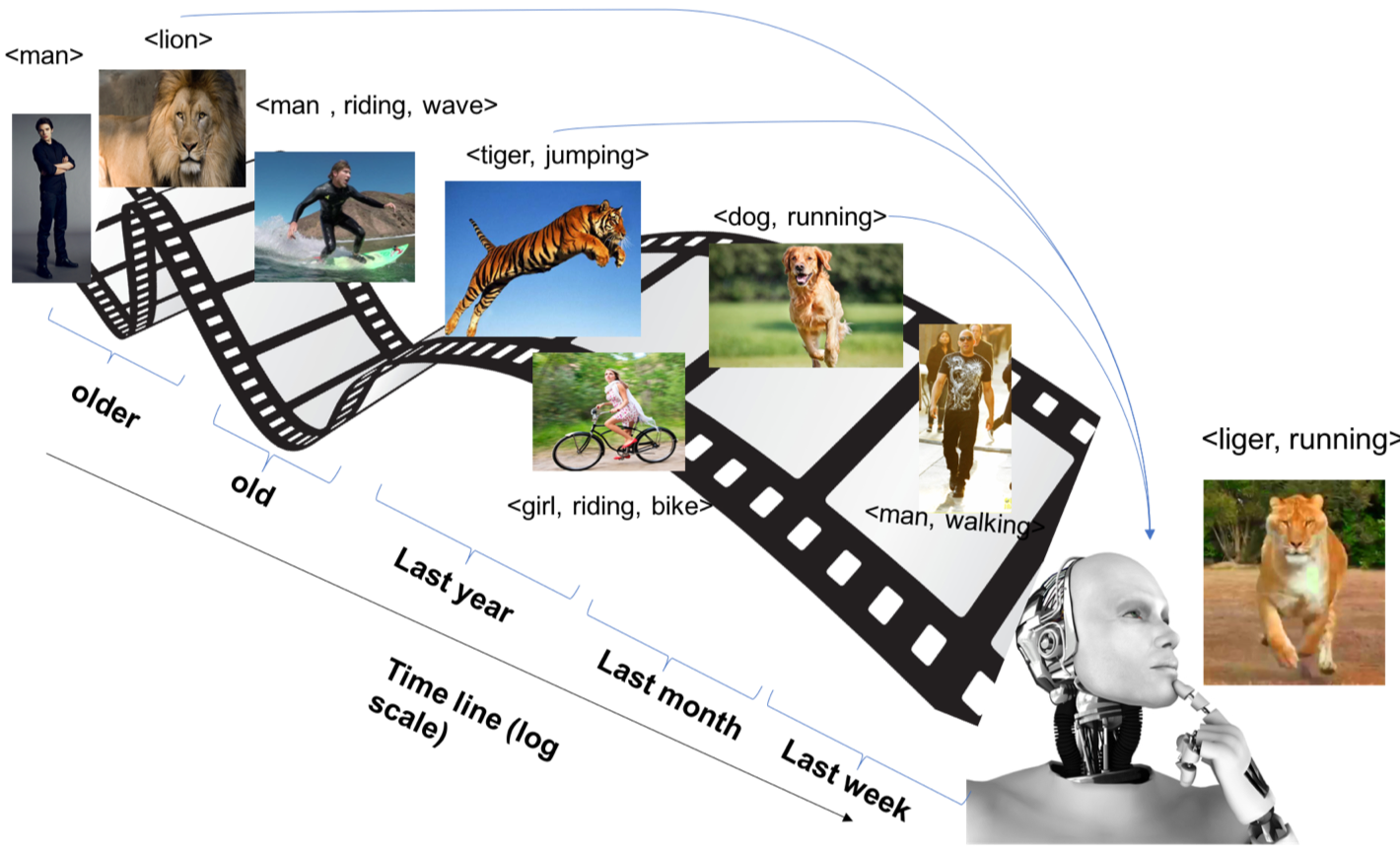
Figure 1: Lifelong Fact Learning

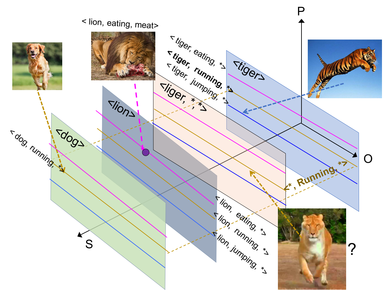
Figure 2: Structured Fact Representation

Lifelong Fact Learning (LLFL). Existing works on LLL have focused mostly on image classification tasks (e.g. [2, 11, 16, 23, 28, 30]), in a relatively small-scale and somewhat artificial setup. A sequence of tasks is defined, either by combining multiple datasets (e.g., learning to recognize MITscenes, then CUB-birds, then Flowers), by dividing a dataset (usually CIFAR100 or MNIST) into sets of disjoint concepts, or by permuting the input (permuted MNIST). Instead, in this work we propose a LLL setup with the following more realistic and desirable learning characteristics:

1. Long-tail: Training data can be highly unbalanced with the majority of concepts occurring only rarely, which is in contrast to many existing benchmarks (e.g.,  [10, 14, 26]).

2. Concepts of varying complexity: We want to learn diverse concepts, including not only objects but also actions, interactions, attributes, as well as combinations thereof.

3. Semantic and structure aware: We want to connect semantically related visual facts. For example, if we have learned “lion” and “tiger” earlier, that can help us later in time to learn a “liger” (a rare hybrid cross between a male lion and a female tiger), even with just a few examples. Relating this to point (2) above, this further allows compositional lifelong learning to help recognize new facts (e.g. $\langle$dog, riding, wave$\rangle$) based on facts seen earlier in time (e.g. $\langle$person, riding, wave$\rangle$ and $\langle$girl, walking, dog$\rangle$).

To the best of our knowledge, none of the existing LLL literature explored these challenges. We denote studying lifelong learning with the aforementioned characteristics as lifelong fact learning (LLFL); see Fig. 2.

A Note on Evaluation Measures. We argue that the evaluation of LLL methods should be reconsidered. In the standard LLL (with a few notable exceptions, such as [2, 4]), the trained models are judged by their capability to recognize each task’s categories individually assuming the absence of the categories covered by the remaining tasks – not necessarily realistic. Although the performance of each task in isolation is an important characteristic, it might be deceiving. Indeed, a learnt representation could be good to classify an image in a restricted concept space covered by a single task, but may not be able to classify the same image when considering all concepts across tasks. It is therefore equally important to measure the ability to distinguish the learnt concepts across all the concepts over all tasks. This is important since the objective of LLL is to model the understanding of an ever growing set of concepts over time. To better understand how LLL performs in real world conditions, we advocate evaluating the existing methods across different tasks. We named that evaluation Generalized lifelong learning (G-LLL), in line with the idea of Generalized zero-shot learning proposed in [3]. We detail the evaluation metric in Sec. 5.1.

Advantages of a Visual-Semantic Embedding. As illustrated in Fig. 2, we expect to better understand $\langle$liger, running$\rangle$ by leveraging previously learnt facts such as $\langle$lion$\rangle$, $\langle$tiger, jumping$\rangle$ and $\langle$dog, running$\rangle$. This shows how both semantics and structure are helpful for understanding. To our knowledge, such semantic awareness has not been studied in a LLL context. To achieve this, we use a visual-semantic embedding model where semantic labels and images are embedded in a joint space. For the semantic representation, we leverage semantic external knowledge using word embeddings – in particular word2vec [19]. These word embeddings were shown to efficiently learn semantically meaningful floating point vector representations of words. For example, the average vector of lion and tiger is closest to liger. This can help semantically similar concepts to learn better from one another, as shown in [31, 7] in non LLL scenarios. Especially in our long-tail setting, this can be advantageous. Additionally, by working with an embedding instead of discrete concept labels as in [8, 15, 12, 30], we avoid that the model keeps growing as new concepts get added, which would make the model less scalable and limit the amount of sharing.

Contributions. First, we introduce a midscale and a large scale benchmark for Lifelong Fact Learning (LLFL), with two splits each, a random and a semantic split. Our approach for creating a semantically divided benchmark is general and could be applied similarly to other datasets or as more data becomes available. Second, we advocate to focus on a more generalized evaluation (G-LLL) where test-data cover the entire label space across tasks. Third, we evaluate existing LLL approaches in both the standard and the generalized setup on our new LLFL benchmarks. Fourth, we discuss the limitations of the current generation of LLL methods in this context, which forms a basis for advancing the field in future research. Finally, this paper aims to answer the following questions: How do existing LLL methods perform on a large number of concepts? What division of tasks is more helpful to continually learn facts at scale (semantically divided vs randomly divided)? How does the long-tail distribution of the facts limit the performance of the current methods?

2 Related Work

Dataset	Structured/Diverse	Long-Tail	Classes	Examples	Task Count	Split Type
MNIST	✗	✗	10	60000	2 to 5	R
CIFAR (used in [23, 30, 18])	✗	✗	100	60000	2 and 5	R
ImageNet and CUB datasets (used in [15])	✗	✗	1200	1211000	2	R
Scenes, CUB, VOC, and Flowers (used in  [16, 2, 28])	✗	✗	122-526	5908-1211000	2	S
8 Dataset Sequence [1]	✗	✗	889	714387	8	S
CORe50  [17] / iCUBWorld-Transf( [21]	✗	✗	10 (50)/15(150)	550/900 sessions	10	S
Our Mid-Scale LLFL Benchmark	✓	✗	186	28624	4	S $\&$ R
Our Large Scale LLFL Benchmark	✓	✓	165150	906232	8	S $\&$ R

Table 1: Comparison of some existing Task Sequences. Split Type is either S (Semantic), R (Random), or S$\&$R (Both Semantic and Random splits are provided)

Previous Evaluations of LLL. In Table 1, we compare some of the popular datasets/ benchmarks used in LLL. As also noted by Rebuffi et al. [23], there is limited agreement about the setup. Most build a task sequence by combining or dividing standard object/scene recognition datasets. In the context of robotics, Lomonaco and Maltoni [17] introduced the CORe50 dataset which consists of relatively short RGB-D video fragments (15sec) of handheld domestic objects. They focus both on category-level as well as instance-level object recognition. With 50 objects belonging to 10 different categories it is, however, relatively small scale and limited in scope. Pasquale et al. with a similar focus proposed the iCUBWorld-Transf dataset [21] with 200 real objects divided in 20 categories. For CORe50 and iCUBWorld-Transf, the number of instances is shown in parenthesis in Table 1. In a reinforcement learning setup, Kirkpatrick et al. [12] and Fernando et al. [8] performed interesting LLL experiments using a sequence of Atari Games as tasks. In contrast to all of the above, we aim at a more natural and a larger-scale setup; see last two rows in Table 1. Our benchmarks are more structured and challenging, due to the large number of classes and the long-tail distribution.

Existing LLL Approaches. LLL works may be categorized into data-based and model-based approaches. In this work, we do not consider methods that require storing samples from previous tasks in an episodic memory [23, 18].

In data-based approaches [16, 25, 28], the new task data is used to estimate and preserve the model behavior on previous tasks, mostly via a knowledge distillation loss as proposed in Learning without Forgetting [16]. These approaches are typically applied to a sequence of tasks with different output spaces. To reduce the effect of distribution difference between tasks, Triki et al. [28] propose to incorporate a shallow auto-encoder to further control the changes to the learned features, while Aljundi et al. [2] train a model for every task (an expert) and use auto-encoders to help determine the most related expert at test time given an example input.

Model-based approaches [8, 15, 12, 30] on the other hand focus on the parameters of the network. The key idea is to define an importance weight $\omega_{i}$ for each parameter $\theta_{i}$ in the network indicating the importance of this parameter to the previous tasks. When training a new task, network parameters with high importance are discouraged from being changed. In Elastic Weight Consolidation, Kirkpatrick et al. [12] estimate the importance weights $\mathbf{\Omega}$ based on the inverse of the Fisher Information matrix. Zenke et al. [30] propose Synaptic Intelligence, an online continual model where $\mathbf{\Omega}$ is defined by the contribution of each parameter to the change in the loss, and weights are accumulated for each parameter during training. Memory Aware Synapses [1] measures $\mathbf{\Omega}$ by the effect of a change in the parameter to the function learned by the network, rather than to the loss. This allows to estimate the importance weights not only in an online fashion but also without the need for labels. Finally, Incremental Moment Matching [15] is a scheme to merge models trained for different tasks. Model-based methods seem particularly well suited for our setup, given that we work with an embedding instead of disjoint output spaces.

3 Our Lifelong Fact Learning Setups

We aim to build two LLL benchmarks that consist of a diverse set of facts (two splits for large-scale and two splits for mid-scale). The benchmarks capture different types of facts including objects (e.g., $\langle$lion$\rangle$, $\langle$tiger$\rangle$), objects performing some activities (e.g., $\langle$tiger, jumping$\rangle$, $\langle$dog,running$\rangle$), and interactions between objects (e.g., $\langle$lion, eating, meat$\rangle$). Before giving details on the benchmark construction, we first explain how we represent facts.

A visual-semantic embedding for facts. Inspired by [22, 7], we represent every fact for our LLL purpose by three pieces represented in a semantic continuous space. $\textbf{S}\in\mathbb{R}^{d}$ represents object or scene categories. $\textbf{P}\in\mathbb{R}^{d}$ represents predicates, e.g. actions or interactions. $\textbf{O}\in\mathbb{R}^{d}$ represents objects that interact with S. Each of S, P, and O lives in a high dimensional semantic space. By concatenating these three representations, we obtain a structured space that can represent all the facts that we are interested to study in this work. Here, we follow [7] and semantically represent each of S, P, and O by their corresponding word2vec embeddings [19].

$$\small\begin{split}\textbf{$\langle$S,P,O$\rangle$ \text{(e.g., <person, riding, horse>)}: }\mathbf{t}=[\mathbf{t}_{S},\mathbf{t}_{P},\mathbf{t}_{O}]\\ \ \textbf{$\langle$S, P,*$\rangle$ \text{ (e.g., <man, walking, *>)}: }\mathbf{t}=[\mathbf{t}_{S},\mathbf{t}_{P},\mathbf{t}_{O}=*]\\ \textbf{ $\langle$S,*,*$\rangle$ \text{(e.g., <dog, *, *>)}: }\mathbf{t}=[\mathbf{t}_{S},\mathbf{t}_{P}=*,\mathbf{t}_{O}=*]\end{split}$$ (1)

where $[\cdot,\cdot,\cdot]$ is the concatenation operation and $*$ means undefined and set to zeros. The rationale behind this notation convention is that if a ground truth image is annotated as $\langle$man$\rangle$, this could also be $\langle$man, standing$\rangle$ or $\langle$man, wearing, t-shirt$\rangle$. Hence, we represent the man as $\langle$man, *,*$\rangle$, where $*$ indicates that we do not know if that “man” is doing something. Figure 2 shows how different fact types could be represented in this space, with S, P, and O visualized as a single dimension. Note that S facts like $\langle$lion$\rangle$ are represented as a hyper plane in this space. While $\langle$tiger, jumping$\rangle$ and $\langle$lion, eating, meat$\rangle$ are represented as a hyper-line and a point respectively.

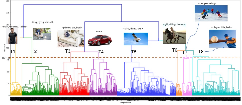
Figure 3: Lifelong Learning Semantically Divided Benchmark: 8 Tasks generated by agglomerative clustering in the semantic space of facts. The method is general and can be re-applied as more images and labels become available.

3.1 Large Scale LLFL Benchmark

We build our setup on top of the large scale fact learning dataset introduced by [7], denoted as Sherlock LSC (for Large SCale). It has more than 900,000 images and 200,000 unique facts, from which we excluded attributes. The dataset was created by extracting facts about images from image descriptions and image scene graphs. It matches our desired properties of being long-tailed and semantic-aware due to its structure.

Given this very large set of facts and examples for each of them, we want to learn them in a LLL setting. This involves splitting the data into a sequence of disjoint tasks (that is, with no overlap in the facts learned by different tasks). However, due to their structured nature, facts may be partially overlapping across tasks, e.g. have the same subject or object. In fact, we believe that some knowledge reappearing across different tasks is a desired property in many real-life LLL settings, as it facilitates knowledge transfer. On the other hand, one could argue that the different tasks that real world artificial agents are exposed to, are likely to cover different domains – a setting more in line with existing LLL works. To study both scenarios, we built a semantically divided split (less sharing among tasks) and a randomly divided one (with more sharing).

Table 2: Number of Unique Facts (i.e., Labels) and Images in each of the 8 tasks for our Semantically and Randomly Divided Large-Scale Benchmark for $\langle$S$\rangle$, $\langle$S,P$\rangle$, and $\langle$S,P,O$\rangle$

Random							Semantic
Task	Facts-SPO	Facts-SP	Facts-S	images-SPO	images-SP	images-S	Task	Facts-SPO	Facts-SP	Facts-S	images-SPO	images-SP	images-S
1	19311	7100	1114	40244	41523	102605	1	6577	224	1	19311	41523	102605
2	16051	5926	961	35265	34234	99442	2	25552	2871	3	16051	34234	99442
3	14594	5305	796	27812	32215	58009	3	12400	517	250	14594	32215	58009
4	13430	4851	761	26069	24701	66355	4	7923	305	46	13430	24701	66355
5	8713	3255	524	18217	17588	100465	5	42264	24381	6321	8713	17588	100465
6	14125	5274	830	30827	32830	57656	6	2819	413	7	14125	32830	57656
7	16688	5935	876	34313	30582	55362	7	6917	1181	4	16688	30582	55362
8	13083	4845	802	28255	27525	366338	8	11543	12599	32	13083	27525	366338
Total	115995	42491	6664	241002	241198	906232	36	115995	42491	6664	115995	241198	906232

Large Scale Semantically Divided Split. We semantically group the facts to create the tasks needed to build our benchmark, i.e. we cluster similar facts and assign each cluster to a task $T_{i}$. In particular, we first populate the structured embedding space with all the training facts and then cluster the facts semantically with a custom metric. Since our setting allows diverse facts where one or two of the three components might be undefined, we need to consider a proper similarity measure to allow clustering the facts. We assume that the structured fact space is Euclidean and has unit norm (i.e., cosine distance). Hence, we define the distance between two facts $\mathbf{t}_{i}$ and $\mathbf{t}_{j}$ as follows:

$$\small\begin{split}D(\mathbf{t}^{i},\mathbf{t}^{j})=&\frac{w_{S}^{ij}\|\mathbf{t}^{i}_{S}-\mathbf{t}^{j}_{S}\|^{2}+w_{P}^{ij}\|\mathbf{t}^{i}_{P}-\mathbf{t}^{j}_{P}\|^{2}+w_{O}^{ij}\|\mathbf{t}^{i}_{O}-\mathbf{t}^{j}_{O}\|^{2}}{w_{S}^{ij}+w_{P}^{ij}+w_{O}^{ij}}\\ w_{l}^{ij}=&0\text{ only if }\mathbf{t}^{i}_{l}=*\text{ or }\mathbf{t}^{j}_{l}=*,l\in\{\textbf{S,P,O}\}\text{ and }w_{l}^{ij}=1\text{ otherwise}.\end{split}$$ (2)

with $w_{l}$ an indicator value distinguishing between singleton facts, pairs or triplets. The intuition behind this distance measure is that we do not want to penalize the $*$ (undefined) part when comparing for example $t_{i}=$$\langle$person,*,*$\rangle$ to $t_{j}=$$\langle$person,jumping,*$\rangle$. In this case the distance should be zero since the $*$ piece does not contribute to the distance measure. We rely on bottom-up hierarchical agglomerative clustering which clusters facts together monotonically based on their distance into disjoint tasks using the aforementioned distance measure. This clustering algorithm recursively merges the pair of clusters that minimally increases a given linkage metric. In our experiments, we use the nearest point algorithm, i.e. clustering with single linkage. An advantage of the agglomerative clustering algorithm is that the distance measure need not be a metric.

The result of the clustering is shown in the form of a Dendrogram in Fig. 3. By looking at the clustered facts, we choose a threshold of 85, shown by the red-dashed line, leading to $n=8$ tasks in our work, as detailed further in Table 2. We attach in the supplementary a PCA visualization of the generated tasks using the word embedding representation of each fact and histogram over facts to illustrate the long-tail. We note that the number of facts and images is not uniform across tasks, and some tasks are likely easier than others. We believe this mimics realistic scenarios, where an agent will have to handle tasks which are of diverse challenges.

Large Scale Randomly Divided Split. We also introduce a randomly divided benchmark where the facts are divided randomly over tasks rather than based on semantics. The semantic overlap between randomly split tasks is expected to be higher than for the semantically-split tasks where the semantic similarity between tasks is minimized. Table 2 shows the task information some further information for both types of splits. For the random split, we make sure that the tasks contain a balanced number of facts and of corresponding training and test images by selecting the most balanced candidate out of 100 random trials. Hence, the random split is more balanced by construction in terms of training images per task. Since we split the data randomly into tasks, semantically related facts would be distributed across tasks.

3.2 Mid Scale Balanced LLFL Benchmark

Compared to the large scale dataset, this dataset is more balanced, with the long-tail effect being less pronounced. This allows us to contrast any change in the behavior of the LLL methods going from a uniform distribution to a long-tail distribution. We build the mid-scale LLFL dataset on top of the 6DS dataset introduced in [7]. It is composed of $186$ unique facts and $28,624$ images, divided in $14,599$ training samples and $14,025$ test samples. We divided this dataset randomly and semantically into 4 tasks.

Mid-Scale Semantic Split. We use the same mechanism for clustering as described above to create a benchmark of 4 tasks that are semantically divided. By visually analyzing the clusters, we find the following distribution: - Task 1: facts describing human actions such as $\langle$person,riding bike$\rangle$, $\langle$person, jumping$\rangle$, - Task 2: facts of different objects such as $\langle$battingball$\rangle$, $\langle$battingstumps$\rangle$, $\langle$dog$\rangle$, $\langle$car$\rangle$, - Task 3: facts describing humans holding or playing musical instruments, such as $\langle$person, playing,flute$\rangle$, $\langle$person, holding, cello$\rangle$, etc. - Task 4: facts describing human interactions such as $\langle$person, arguing with, person$\rangle$, $\langle$person, dancing with, person$\rangle$.

Mid-Scale Random Split. We followed the same procedure described in the large scale benchmarks to split the facts into 4 different random groups. Note that [1] evaluated image retrieval (with average precision) on a similar random-split of 6DS [7] while in this work we look at the task of fact recognition (measured in accuracy), which is meaningful for both the mid-scale and the large-scale benchmarks (our focus) since the vast majority of the facts has only one image example.

4 Lifelong Learning Approaches

In this section, we first formalize the life-long learning task, then we review the evaluated methods, and finally we explain how we adapt them to fact learning.

4.1 LLL Task

Given a training set $\mathcal{D}=\{(\mathbf{x}_{k},y_{k})\}_{k=1}^{M}$, we learn from different tasks $T_{1},T_{2},\ldots,T_{N}$ over time where $T_{n}\subset\mathcal{D}$. $y_{k}$ in our benchmarks are structured labels. For most model-based approaches, we can formalize the LLL loss as follows. The loss of training the new $n^{th}$ task is $L_{n}(\theta)$, where $\theta$ are the parameters of the network such that $\theta_{i}$ is the $i^{th}$ parameter of an arbitrary neural network (a deep neural network with both convolutional and fully connected layers, in our case). $L(\theta)$ is defined as $L(\theta)=L_{n}(\theta)+\frac{\lambda}{2}\sum_{i}\omega^{n-1}_{i}(\theta_{i}-\theta^{n-1}_{i})^{2}$, where $\lambda$ is a hyperparameter for the regularizer, $\theta_{i}^{n-1}$ the previous task’s network parameters, and $\omega_{i}^{n-1}$ a weight indicating the importance of parameter $\theta_{i}$ for all tasks up to $n-1$. Hence, we strongly regularize the important parameters at the previous time step (i.e., high $\omega^{n-1}_{i}$) and weak regularization on the non-important parameters (i.e., low $\omega^{n-1}_{i}$). This way, we allow changing the latter more freely. Under this importance weight based framework, Finetuning, Intelligent Synapses [30] and Memory Aware Synapses [1] are special cases.

4.2 Evaluated Methods

(1) Finetuning (FT): FT is a common LLL baseline. It does not involve any importance parameters, so $\omega^{n}_{i}=0,\forall i$.

(2) Synaptic Intelligence [30] (Int.Synapses) estimates the importance weights in an online manner while training based on the contribution of each parameter to the change in the loss. The more a parameter $\theta_{i}$ contributes to a change in the loss, the more important it is.

(3) Memory Aware Synapses [1] (MAS) defines importance of parameters in an online way based on their contribution to the change in the function output. $\omega_{i}^{n}=\frac{1}{M_{n}}\sum_{k=1}^{M_{n}}\mid\mid g_{i}(x_{k})\mid\mid$, where $g_{i}(x_{k})=\frac{\partial(F(x_{k};\theta))}{\partial\theta_{i}}$ is the gradient of the learned function with respect to $\theta_{i}$ evaluated at the data point $x_{k}$. $F$ maps the input $X_{i}$ to the output $Y_{i}$. This mapping is the target that MAS preserves to deal with forgetting.

(4) ExpertGate [2]. ExpertGate is a data-based approach that learns an expert model for every task $E_{1},E_{2},\cdots E_{n}$, where every expert is adapted from the most related task. An auto-encoder model is trained for every task $AE_{1},AE_{2},\cdots AE_{n}$. These auto-encoders help determine the most related expert at test time given an example input $x$. The expert is then to make the prediction on $x$. Note the memory storage requirements of ExpertGate is $n$ times the number of parameters of a single model which might limit its practicality.

(5) Incremental Moment Matching [15] (IMM). For $N$ sequential tasks, IMM finds the optimal parameter $\mu^{*}_{1:N}$ and $\Sigma^{*}_{1:N}$ of the Gaussian approximation function $q_{1:N}$ from the posterior parameter for each $n^{th}$ task, $(\mu_{n},\Sigma_{n})$. At the end of the learned sequence, the obtained models are merged through a first or second moment matching. Similarly to ExpertGate, IMM needs to store all models - at least if one wants to be able to add more tasks in the future. We find the mode IMM to work consistently better than the mean IMM so we report it in our experiments.

(6) Joint Training (Joint): In joint training, the data is not divided into tasks and the model is trained on the entire training data at once. As such, it violates the LLL assumption. This can be seen as an upper bound for all LLL methods that we evaluate.

4.3 Adapting LLL methods to fact learning

We use the joint-embedding architecture proposed in [7] as our backbone architecture to compare the evaluated methods. We chose this architecture due its superior performance compared to other joint-embedding models like [9, 13, 24] and its competitive performance to multi-class cross-entropy. The main difference between joint embedding models and standard classification models is in the output layer. Instead of a softmax output, the last layer in a joint-embedding model consists of a projection onto a joint embedding space. This allows exploiting the semantic relation between facts as well as the structure in the data, as explained before. However, as discussed in the related work section, this is problematic for some of the LLL methods, such as [15, 28] that assume a different output space for each task. This makes the problem challenging and may raise other forgetting aspects. Note that we used the same data loss term in all the evaluated methods in the previous section.

5 Experiments

We first present the evaluation metrics, then evaluate the different methods on our benchmarks and discuss the results, and finally we provide a more detailed analysis on long-tail, knowledge acquisition over time, and few-shot learning.

5.1 Fact Learning Evaluation metrics

Evaluation Metric (Standard vs Generalized). A central concept of LLL is that at a given time $n$ we can only observe a subset $T_{n}$ of the labeled training data $T_{n}=\{(\mathbf{x}_{k},y_{k})\}_{k=1}^{M_{n}}\subset\mathcal{D}$ . Over time, we learn from different tasks $T_{1},T_{2},\ldots,T_{N}$. The categories in the different tasks are not intersecting, i.e., if $Y_{n}$ is the set of all category labels in task $T_{n}$ then $Y_{n}\cap Y_{n^{\prime}}=\emptyset,\forall n\neq n^{\prime}$. Let $\mathcal{Y}$ denote the entire label space covered by all tasks, i.e., $\mathcal{Y}=\cup{Y_{n}},\forall n$. Many existing works assume that one does not have to disambiguate between different tasks, i.e. for a predictive function $f_{y}:X\mapsto\mathbb{R}$, we compute $A_{T_{n}\to{Y}_{n}}$ as the accuracy of classifying test data from $T_{n}$ (the ${n^{th}}$ task) into ${Y}_{n}$ (the label space of ${T}_{n}$). The accuracy is computed per task.

$$\vspace{-2mm}\small\textbf{Standard LLL (S-LLL) Accuracy: }A_{T_{n}\to{Y}_{n}}=\frac{1}{M_{n}}\sum_{n}^{M_{n}}1[y_{k}=\arg\max_{y^{\prime}\in{Y}_{n}}f_{y^{\prime}}(x_{k})]$$ (3)

where $y_{k}$ is the ground truth label for instance $x_{k}$. This metric assumes that at test time one knows the task of the input image. This is how most existing works are evaluated. However, this ignores the fact that determining the right task can be hard, especially when tasks are related. Therefore, we also evaluate across all tasks, which we refer to as Generalized LLL.

$$\small\textbf{Generalized LLL (G-LLL) Accuracy: }A_{T_{n}\to\mathcal{Y}}=\frac{1}{M_{n}}\sum_{k}^{M_{n}}1[y_{k}=\arg\max_{y^{\prime}\in\mathcal{Y}}f_{y^{\prime}}(x_{k})]\vspace{-2mm}$$ (4)

In the generalized LLL metric, the search space at evaluation time covers the entire label space across tasks (i.e., $\mathcal{Y}$). Hence, we compute $A_{T_{n}\to\mathcal{Y}}$ as the accuracy of classifying test data from $T_{n}$ (the ${n^{th}}$ task) into $\mathcal{Y}$ (the entire label space) which is more realistic in many cases. In our experiments, $f_{y}(x)$ is a visual-semantic embedding model, i.e., $f_{y}(x)=s(\phi(x),\psi(y))$ where $s(\cdot,\cdot)$ is a similarity function between the visual embedding of image $x$ denoted by $\phi(x)$ and the semantic embedding of label $y$ denoted by $\psi(y)$. $\phi(x)$ is typically a CNN sub-network and $\psi(y)$ is a semantic embedding function of the label $y$ (e.g., word2vec [19]). The above two metrics can easily be generalized to Top K standard and generalized accuracy that we use in our experiments.

For each metric, we summarize results by averaging over tasks (“mean”) and over examples (“mean over examples”), creating slightly different results when tasks are not balanced.

Similarity Measure between Tasks (word2vec, SPO overlap). As an analysis tool, we measure similarity between tasks in both the Semantic and the Random splits using two metrics. In the first metric, the similarity is measured by the cosine similarity between average word2vec representation of the facts in each task. In the second metric, we computed the overlap between the two tasks, separately for S, P, and O. For example, to compute the overlap in S, we first compute the number of intersecting unique subjects and divide that by the union of unique subjects in both tasks. This results in a ratio between 0 and 1 that we compute for subjects and similarly for objects and predicates. Based on these three ratios, we compute their geometric mean as an indicator for the similarity between the two tasks. We denote this measure as the SPO overlap.

5.2 Results

In this section we compare several state-of-the art LLL approaches on the mid-scale and the large-scale LLL benchmark which we introduced in Sec. 3. Tables 3 and 4 show the Top5 accuracy for the random and the semantic splits on the mid-scale dataset. Each table shows the performance using the standard metric (Eq.  3) and the generalized metric (Eq. 4). For the two large-scale benchmarks, the results are reported in Tables 5, 6  7 and  8. Note that the reported Joint Training violates the LLL setting as it trains on all data jointly. Looking at these results, we make the following observations:

Random Split	standard metric						generalized metric						Drop (standard to generalized)
	T1	T2	T3	T4	mean	mean over examples	T1	T2	T3	T4	mean	mean over examples	over tasks	over examples
ExpertGate	79.6	59.25	62.92	58.75	65.13	64.88	53.1	44.83	37.03	40.66	43.9	43.69	21.22	21.18
FineTune	76.41	46.18	52.44	88.32	65.84	66.11	42.06	22.5	17.84	83.15	41.39	42.02	24.45	24.09
IMM	85.2	75.15	83.66	69.27	78.32	78.15	63.39	62.13	67.58	43.06	59.04	58.77	19.28	19.38
Int.Synapses	82.31	65.28	68.64	87.03	75.81	75.94	49.37	39.92	38.45	74.52	50.57	50.95	25.25	24.98
MAS	86.76	70.89	75.87	85.06	79.65	79.68	55.23	48.62	51.1	71.72	56.67	56.94	22.98	22.74
Joint	88.66	78.38	87.82	75.91	82.69	82.57	75.81	68.45	79.03	60.82	71.03	70.87	11.67	11.7

Table 3: Mid-scale Dataset (Random Split) Top 5 Accuracy

Semantic Split	standard						generalized						Drop (standard to generalized)
	T1	T2	T3	T4	mean	mean over examples	T1	T2	T3	T4	mean	mean over examples	over tasks	over examples
ExpertGate	62.11	62.44	59.4	12.5	49.11	59.39	55.57	50.87	49.61	9.49	41.38	51.83	7.73	7.57
FineTune	16.24	35.63	31.71	15.19	24.69	21.3	8.25	0	0	15.19	5.86	6.07	18.83	15.24
IMM	64.26	87.52	63.27	12.82	56.97	64.33	38.75	30.16	43.28	8.70	30.22	37.31	26.74	27.02
Int.Synapses	16.48	35.69	32.01	8.54	23.18	21.23	8.25	0	0	8.54	4.2	5.77	18.98	15.46
MAS	28.19	47.91	34.8	12.97	30.97	30.96	8.34	0.13	0	12.97	5.36	6.04	25.61	24.92
Joint	80.14	53.12	81.47	21.2	58.98	74.75	77.34	39.55	79.2	18.99	53.77	70.87	5.22	3.87

Table 4: Mid-scale Dataset (Semantic Split)

Random	T1	T2	T3	T4	T5	T6	T7	T8	mean	mean over examples
ExpertGate	16.37	20.49	28.36	22.2	37.75	12.52	14.14	24.37	22.02	20.95
Finetune	15.53	23.56	23.43	19.22	23.44	19.53	23.81	66.13	26.83	26.59
IMM	24.57	30.72	32.14	27.89	37.23	25	20.65	26.41	28.08	27.53
Int.Synapses	18.28	27.23	27.11	23.3	28.85	23.49	25.76	53.43	28.43	28.06
MAS	21.32	33.32	32.82	28.58	34.93	27.16	29.71	52.22	32.5	32.00

Table 5: Large Scale Random Split (Standard Performance) Top 5 Accuracy

Random	T1	T2	T3	T4	T5	T6	T7	T8	mean	mean over examples
ExpertGate	12.99	20.77	25.19	17.72	35.17	9.62	11.64	21.75	19.36	15.34
Finetune	12.18	21.38	19.98	15.68	19.85	16.11	17.48	59.29	22.74	18.93
IMM	21.21	29.02	30.5	25.38	34.01	23.42	18.07	24.26	25.73	20.91
Int.Synapses	13.79	24.99	23.58	19.01	26.4	21.56	20.95	47.69	24.75	19.92
MAS	16.13	29.52	28.28	23.1	30.28	24.5	24.34	47.21	27.92	22.48

Table 6: Large Scale Random Split (Generalized Performance) Top 5 Accuracy

(1) The generalized LLL accuracy is always significantly lower than the standard LLL accuracy. On the large scale benchmarks it is on average several percent lower: $7.99\%$ and $11.59\%$ for the random and the semantic splits, respectively. While the large-scale benchmarks are more challenging than the mid-scale benchmarks, as apparent from the reported accuracies, the drop in performance when switching to the generalized accuracy on the mid-scale benchmarks is significantly larger: $20.59\%$ and $18.16\%$, respectively. This could be due to more overlap between tasks on the large-scale dataset as we discuss later, which reduces forgetting leading to better discrimination across tasks.

(2) The LLL performance of the random split is much better compared to the semantic split. Note that the union of the test examples across tasks on both splits are the same. Hence, the ‘mean over examples” performance on the random and semantic splits are comparable. Looking at the performance of the evaluated methods on both random and semantic splits on the large scale dataset, the average relative gain in performance over the methods by using the random split instead of the semantic split is $61.74\%$ for the generalized metrics. This gain is not observed for ExpertGate which has only $2.77\%$ relative gain when moving to the random split (small compared to other methods). We discuss ExpertGate behavior in a separate point below. The same ratio goes up to $569.03\%$ on the mid-scale dataset excluding ExpertGate. What explains these results is that the similarity between tasks in the random split is much higher in the large-scale dataset compared to the mid-scale dataset (i.e., 0.96 vs 0.22 using the word2vec metric and 0.84 vs 0.25 using the SPO metric – see Table 9 for the task correlation in the LSc dataset and the corresponding table for the mid-scale dataset in the supplementary. This shows the learning difficulty of the semantic split and partially explains the poor performance.

Semantic	T1	T2	T3	T4	T5	T6	T7	T8	mean	mean over examples
ExpertGate	6.97	11.01	35.6	34.61	14.58	21.32	16.36	13.28	19.22	20.15
Finetune	5.55	11.17	13.65	24.04	10.84	12.68	19.41	39.41	17.09	17.91
IMM	9.49	9.25	16.90	30.95	11.05	33.92	18.2	10.99	17.59	14.81
Int.Synapses	5.47	13.3	14.95	25.23	12.43	14.4	20.18	29.8	16.97	17.49
MAS	6.36	14.16	19.51	26.25	13.25	15.22	20.57	28.59	17.99	18.75
Joint	11.62	5.90	36.26	37.56	28.16	16.16	14.32	12.85	20.35	23.41

Table 7: Large Scale Semantic Split (Standard Performance) Top 5 Accuracy

Semantic	T1	T2	T3	T4	T5	T6	T7	T8	mean	mean over examples
ExpertGate	5.18	7.62	35.33	20.35	8.99	16.59	6.21	7.19	13.43	14.91
Finetune	1.58	8.56	0.07	2.06	5.88	2.86	4.77	37.9	7.96	9.75
IMM	8.34	5.06	0.18	13.27	0.52	21.48	11.21	3.26	7.91	4.15
Int.Synapses	1.71	10.82	0.22	2.84	5.87	4.77	6.36	28.26	7.61	8.70
MAS	1.79	11.35	0.64	4.25	4.76	5.36	6.2	27.35	7.71	8.54
Joint	10.20	4.86	37.71	33.52	25.09	3.17	4.83	8.43	15.98	20.68

Table 8: Large Scale Semantic Split (Generalized Performance) Top 5 Accuracy

Semantic(0.07 mean similarity)									Random (0.96 mean similarity)
x	T1	T2	T3	T4	T5	T6	T7	T8		T1	T2	T3	T4	T5	T6	T7	T8
T1	1	0.32	-0.28	-0.18	-0.45	0.23	0.16	0.15	T1	1	0.97	0.97	0.97	0.95	0.97	0.97	0.97
T2	0.32	1	-0.37	-0.11	-0.68	0.21	0.36	0.29	T2	0.97	1	0.97	0.95	0.95	0.96	0.96	0.96
T3	-0.28	-0.37	1	0.25	0.05	-0.26	-0.22	-0.52	T3	0.97	0.97	1	0.97	0.95	0.96	0.97	0.96
T4	-0.18	-0.11	0.25	1	-0.08	-0.01	-0.12	-0.41	T4	0.97	0.95	0.97	1	0.95	0.95	0.97	0.96
T5	-0.45	-0.68	0.05	-0.08	1	-0.26	-0.36	-0.04	T5	0.95	0.95	0.95	0.95	1	0.95	0.96	0.93
T6	0.23	0.21	-0.26	-0.01	-0.26	1	0.23	0.26	T6	0.97	0.96	0.96	0.95	0.95	1	0.96	0.96
T7	0.16	0.36	-0.22	-0.12	-0.36	0.23	1	0.35	T7	0.97	0.96	0.97	0.97	0.96	0.96	1	0.95
T8	0.15	0.29	-0.52	-0.41	-0.04	0.26	0.35	1	T8	0.97	0.96	0.96	0.96	0.93	0.96	0.95	1
Semantic (0.238 g-mean of S,P, and O overlap)									Random (0.453 g-mean of S,P, O overlap)
T1	1	0.09	0.08	0.11	0.05	0.06	0.1	0.08	T1	1	0.39	0.38	0.38	0.35	0.39	0.4	0.38
T2	0.09	1	0.12	0.15	0.15	0.08	0.27	0.28	T2	0.39	1	0.38	0.37	0.35	0.37	0.38	0.38
T3	0.08	0.12	1	0.23	0.2	0.04	0.12	0.1	T3	0.38	0.38	1	0.38	0.36	0.38	0.4	0.38
T4	0.11	0.15	0.23	1	0.15	0.08	0.14	0.12	T4	0.38	0.37	0.38	1	0.37	0.37	0.37	0.37
T5	0.05	0.15	0.2	0.15	1	0.05	0.12	0.18	T5	0.35	0.35	0.36	0.37	1	0.36	0.37	0.36
T6	0.06	0.08	0.04	0.08	0.05	1	0.12	0.1	T6	0.39	0.37	0.38	0.37	0.36	1	0.38	0.38
T7	0.1	0.27	0.12	0.14	0.12	0.12	1	0.28	T7	0.4	0.38	0.4	0.37	0.37	0.38	1	0.38
T8	0.08	0.28	0.1	0.12	0.18	0.1	0.28	1	T8	0.38	0.38	0.38	0.37	0.36	0.38	0.38	1

Table 9: Large Scale Task Similarities using average Word2vec space (top-part) and geometric mean S,P, and O overlap (bottom-part)

(3) ExpertGate is the best performing model on the semantic split. However, it is among the worst performing models on the random split. We argue that this is due to the setup of the semantic split, where sharing across tasks is minimized. This makes each task model behave like an expert of a restricted concept space, which follows the underlying assumption of how ExpertGate works. However, this advantage comes at the expense of storing one model for every task which can be expensive w.r.t. storage requirements which might not always be feasible as the number of tasks increases. Additionally, having separate models, requires to select a model at test time and also removes the ability to benefit from knowledge learnt with later tasks, in case there is a semantic overlap between tasks. This can be seen on the random split on the mid-scale dataset (see Table 3) where ExpertGate underperforms several other LLL models: 43.69% generalized accuracy for ExpertGate vs 58.77% generalized accuracy for the best performing model. Similarly on the large scale dataset, ExpertGate performs significantly lower for the random split (15.34% generalized accuracy for ExpertGate vs 22.48% generalized accuracy for the best performing model); see Table 8. The shared information across tasks on the random split is high which violates the assumption of expert selection in the ExpertGate method and hence explains its relatively poor performance on the random split.

(4) For the midscale dataset and with the generalized metric, Incremental Moment Matching (IMM) is the best performing of the model-based methods using a single model (Finetune, IMM, Int.Synapses, MAS) on both the random and the semantic splits (see Tables 3,4). Only for the random split evaluated with the standard metric MAS is slightly better, indicating that MAS might be better at the task level. We hypothesize that IMM benefits from its access to the distribution of the parameters after training each task before the distributions’ mode is computed. This is an advantage that MAS and Int.Synapses do not have and hence the IMM model can generalize better across tasks. For the large-scale dataset, we observe that MAS is performing better than IMM on both the random and the semantic split, but especially on the random split; see Table 6. This may be because MAS has a better capability to learn low-shot classes as we discuss later in our Few-shot Analysis; see tables 12 and  12. This is due to the high similarity between the tasks as we go to that much larger scale; see Table 9. This makes the distribution of parameters that work well across tasks similar to each other and hence IMM no longer has the aforementioned advantage.

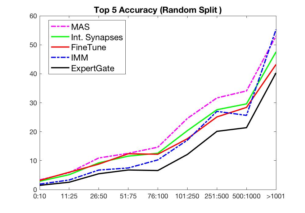
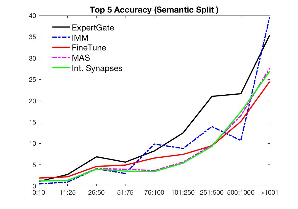
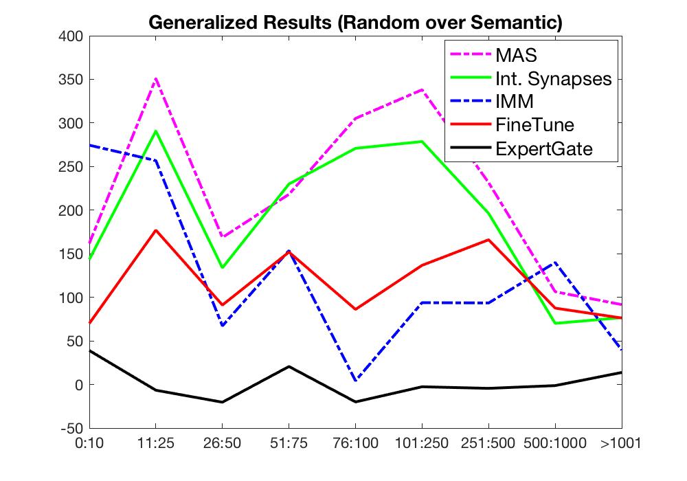
Figure 4: LLFL Benchmark Long-tail analysis (Generalized Results). The x-axis in this figure shows the range of examples seen during training. On the left and middle: the y-axis shows the generalized Top 5 Accuracy for the random and the semantic splits. On the right: The y-axis shows the Random split improvement over the random split for each range.

5.3 Detailed Analysis

Long-tail Analysis. We show in Fig 4 on left and middle the head-to-tail performance on the random split and the semantic split respectively. Specifically, the figure shows the Top5 generalized accuracy over different ranges of seen examples per class (i.e., the x-axis in the figure). On the right, the figure shows the relative improvement of the model trained on the random split over the semantic split. Using the standard metrics, the head classes perform better using models trained on the semantic split compared to the random split. It also shows that the random splits benefit the tail-classes the most; shown in supplementary materials (Section 4). However as shown on Fig 4 (right), random split benefits everywhere with no clear relation to the class frequency (x-axis).

Gained Knowledge Over Time. Figure 5 shows the gained knowledge over time measured by the generalized Top5 Accuracy of the entire test set of all tasks after training each task. Figure 5 (left) shows that the LLL methods tend to gain more knowledge over time when the random split is used. This is due to the high similarity between tasks which makes the forgetting over time less catastrophic. Figure 5 (right) shows that the models have difficulty gaining knowledge over time when the semantic split is used. This is due to the low similarity between tasks which makes the forgetting over time more catastrophic. Note that the y-axis in Figure 5 left and right parts are comparable since it measure the performance of the entire test set which is the same on both the semantic and the random splits.

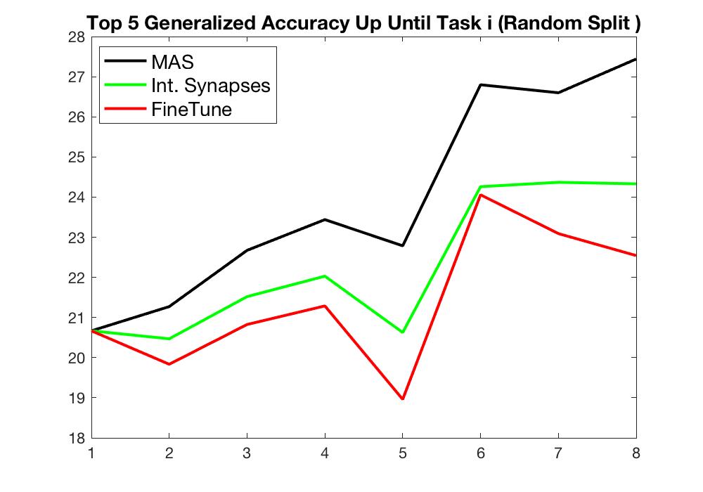
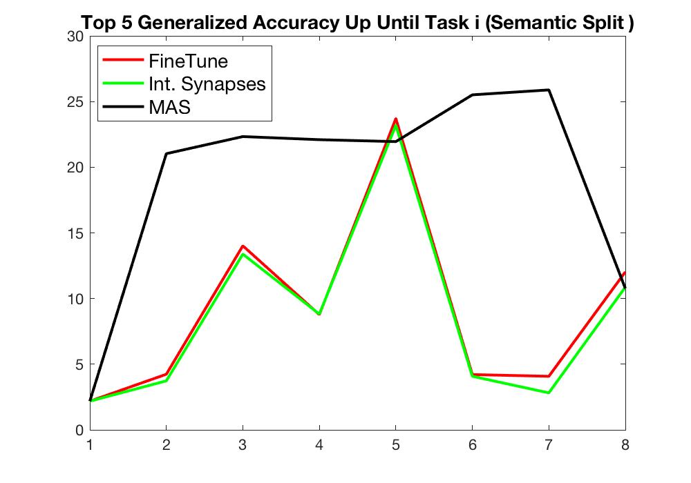
Figure 5: Gained Visual Knowledge: The x-axis shows the task number i. The y-axis shows the Top5 generalized accuracy over the entire test set up until training task i, for the random (left) and semantic (right) split respectively.

For a principled evaluation, we consider measuring the forward and the backward transfer as defined in [18]. After each model finishes learning about the task $T_{n}$, we evaluate its test performance on all $N$ tasks. By doing so, we construct the matrix $R\in\mathbb{R}^{N\times N}$, where $R_{j,n}$ is the test classification accuracy of the model on task $T_{j}$ after observing the last sample from task $T_{n}$. Letting $\bar{b}$ be the vector of test accuracies for each task at random initialization, we can define the backward and the forward transfer as: $\text{ {\bf Backward Transfer: } \normalsize BWT}=\frac{1}{N-1}\sum_{n=1}^{N-1}R_{n,N}-R_{n,n}$ and $\text{ {\bf Forward Transfer: } \normalsize FWT}=\frac{1}{N-1}\sum_{n=2}^{N}R_{n,n-1}-\bar{b}_{n}$. The larger these metrics, the better the model. If two models have similar accuracy, the most preferable one is the one with larger BWT and FWT. We used the generalized accuracy for computing BWT and FWT.

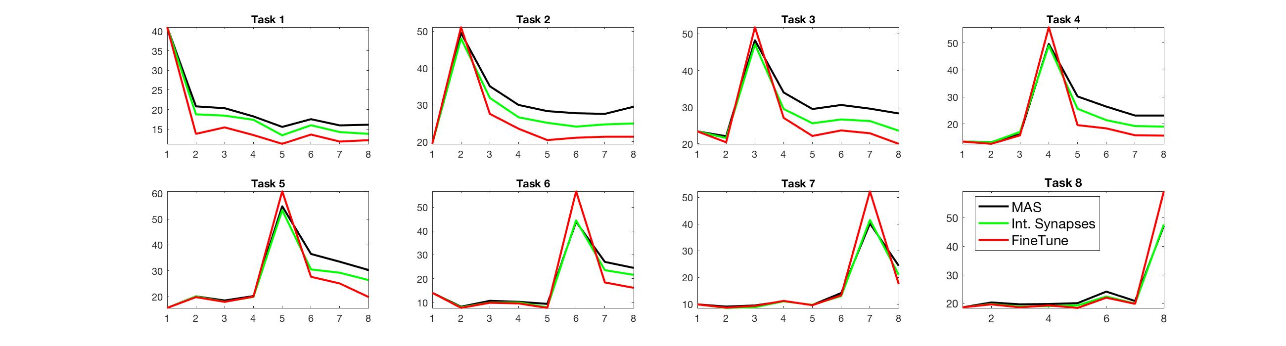
Figure 6: Gained Visual Knowledge broken down for each task on the random split: The x-axis in each sub figure shows the task number i. The y-axis shows the Random Split Top5 generalized accuracy of the shown task after each task is learnt.

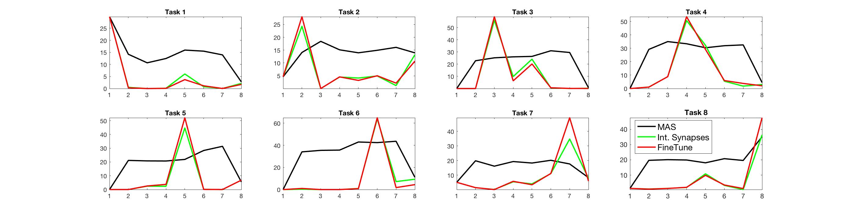
Figure 7: Gained Visual Knowledge broken down for each task on the semantic split: The x-axis in each sub figure shows the task number i. The y-axis shows the Random Split Top5 generalized accuracy of the shown task after each task is learnt.

Semantic	MAS	Int.Synapses	Finetune
Forward Transfer	0.24	0.08	0.06
Backward Transfer	-0.20	-0.37	-0.44
Random	MAS	Int.Synapses	Finetune
Forward Transfer	0.30	0.26	0.22
Backward Transfer	-0.22	-0.25	-0.35

Table 10: Large Scale Benchmark Forward and Backward Transfer for continual learning methods

Figures 6 and  7 show the performance of each task test set after training each task (from first task to last task). As expected the performance on the task $n$ set peaks after training task $n$ and the performance degrades after training subsequent tasks. Int.Synapses and Finetune show the best performance of training the current task at the expense of more forgetting on previous tasks compared to MAS. Comparing the performance of task $n$ at the $n^{th}$ task training to its performance after training the last task as a measure of forgetting, we can observe a lower drop on the performance on the random split compared to the semantic split; see the figures. This is also demonstrated by higher backward transfer on the random split; see Table 10.

Few-shot Analysis. Now, we focus on analyzing the subset of the testing examples belonging to facet with few training examples. Tables  12 and  12 show few-shot results on the semantic and the random split, respectively. As already observed earlier, the performance on the random splits is better compared to the semantic splits. We can observe here that finetuning is the best performing approach on average for few-shot performance on both splits. Looking closely at the results, it is not hard to see that the main gain of finetuning is due to its high accuracy on the last task. This shows that existing LLL methods do not learn the tail and there is need to devise new methods that have a capability to learn the tail distribution in a LLL setting.

	T1	T2	T3	T4	T5	T6	T7	T8	average
ExpertGate	0.33	0.88	0.57	3.27	0.69	2.04	0	0.62	1.05
Finetune	0	0.65	0	0	0.3	2.04	1.76	10.14	1.86
IMM	1.3	0.03	0	0	0.04	2.65	0	0	0.5
Int.Synapses	0.11	0.37	0	0	0.28	2.65	1.14	4.91	1.18
MAS	0.11	0.31	0	0.05	0.22	3.67	1.24	4.58	1.27
Joint	5.55	2.65	4.79	6.27	2.85	10.9	8.88	3.7	5.7

Table 11: Few-shot ($\leq 10$) generalized Top 5 accuracy, Large-scale, Semantic Split

	T1	T2	T3	T4	T5	T6	T7	T8	average
ExpertGate	1.54	1.41	2.51	1.69	0.9	1.58	1.13	0.91	1.46
Finetune	1.48	1.62	1.4	1.73	1.47	1.77	2.66	13.17	3.16
IMM	1.79	1.58	2.1	1.9	2.88	2.07	1.76	0.95	1.88
Int.Synapses	1.4	1.55	2.25	2.95	2.94	3.09	3	5.8	2.87
MAS	1.79	2.29	3.25	3.8	4.6	3.09	3.4	4.44	3.33
Joint	3.75	4.65	6.99	4.61	3.81	8.9	10.38	2.5	5.7

Table 12: Few-shot ($\leq 10$) generalized Top 5 accuracy, Large-scale, Random Split

6 Conclusions

In this paper, we proposed two benchmarks to evaluate fact learning in a lifelong learning setup. A methodology was designed to split up an existing fact learning dataset into multiple tasks, taking the specific constraints into account and aiming for a setup that mimics real world application scenarios. With these benchmarks, we hope to foster research towards more large scale, human-like artificial visual learning systems and studying challenges like long-tail distribution.

Acknowledgements Rahaf Aljundi’s research was funded by an FWO scholarship.

Appendix

In the supplementary, we attach two folders that include the large-scale and mid-scale benchmarks annotations that we developed; see “large-scale_benchmarks” and “large-scale_benchmarks”folders. These folders have a comprehensive list of the tasks and the names of the facts of each of the Large-scale and mid-scale benchmarks. This document also includes additional details and results, listed below.

1. Mid-scale Task Similarities using average Word2vec space

2. Large Scale Semantic Splits 8 Tasks on word2vec space

3. Standard Accuracy (Long Tail/and Semantic/Random Improvement)

4. Long Tail Distribution Statistics on The Large Scale Dataset

5. SPO Generalization

6. Qualitative Examples

7. Mid-Scale dataset Dendogram

7 Mid-scale Task Similarities using average Word2vec space (top-part) and geometric mean S,P, and O overlap (bottom-part)

Semantic (0.02 word2vec mean similarity )					Random (0.22 mean similarity )
	T1	T2	T3	T4		T1	T2	T3	T4
T1	1.00	-0.16	0.04	-0.55	T1	1.00	0.16	0.39	-0.31
T2	-0.16	1.00	-0.22	-0.42	T2	0.16	1.00	-0.12	-0.37
T3	0.04	-0.22	1.00	-0.5	T3	0.39	-0.12	1.00	-0.01
T4	-0.55	-0.42	-0.5	1.00	T4	-0.31	-0.37	-0.01	1.00
Semantic (0.25 g-mean of S,P, and O overlap )					Random (0.84 g-mean of S,P, and O overlap)
	T1	T2	T3	T4		T1	T2	T3	T4
T1	1	0.0792	0.0774	0	T1	1	0.19	0.23	0.12
T2	0.0792	1	0	0	T2	0.19	1	0.19	0.19
T3	0.0774	0	1	0	T3	0.23	0.19	1	0.13
T4	0	0	0	1	T4	0.12	0.19	0.13	1

Table 13: Mid scale Task Similarities using average Word2vec space (top-part) and geometric mean S,P, and O overlap (bottom-part)

7.1 Large Scale Semantic Splits 8 Tasks on word2vec space

Figure 8: LSC Semantic Splits 8 Tasks on word2vec space (900 dimensions using PCA, each Task is color coded by a different color)

7.2 Standard Accuracy (Long Tail/and Semantic/Random Improvement

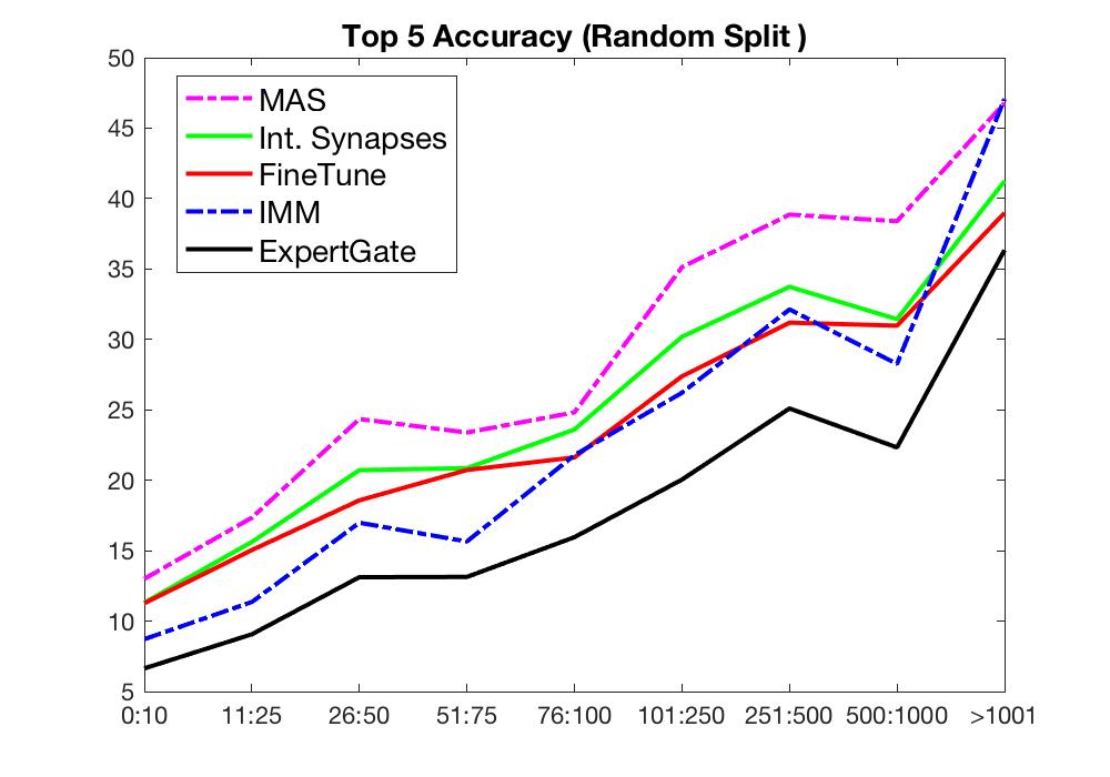
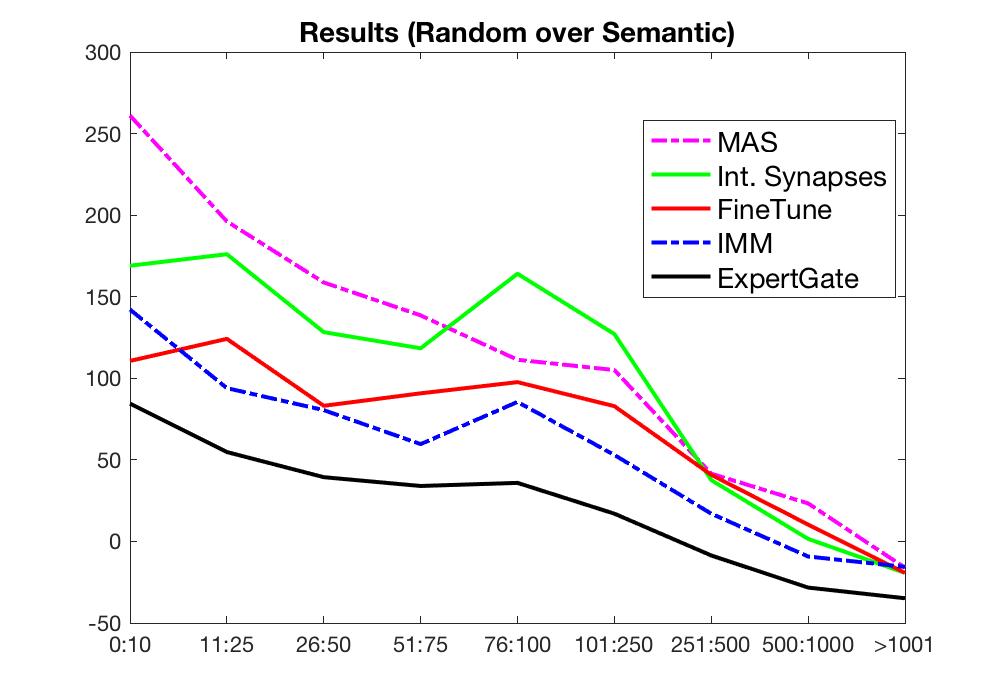
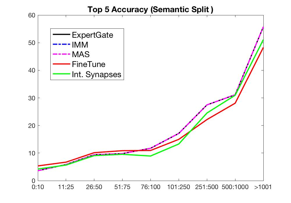
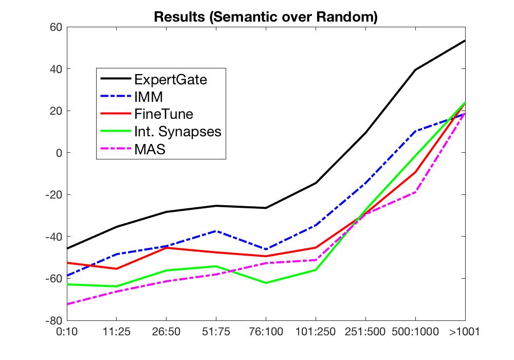
Figure 9: The x-axis in this figure shows the number of examples seen during training. On the left: the y-axis shows the standard Top 5 Accuracy for the random and the semantic splits. On the right: The y-axis shows the Random split improvement over the semantic split for each range and vice versa.

7.3 SPO Generalization

It is desirable for each Life-long learning method to be able to generalize to understand an SPO interaction from training examples involving its components, even when there are zero or very few training examples for the exact SPO with all its parts S,P and O. For example, for $<$dog, riding, horse$>$ SPO example $<\cdot$, riding, horse$>$ (the PO part) might have been seen more than 15 examples (TH=15) and $<$dog,$\cdot$ ,$\cdot>$ the S part might have been seen more than 15 examples. Table  14 and  15 shows the Top5 performance for SPOs for different LLL methods where the number of training examples is $\leq$ 5 for generalization cases where SP$\geq$15,O$\geq TH$, or P$\geq TH$,SO$\geq TH$, or PO$\geq$15,S$\geq TH$, $TH=15$ and $TH-50$ for Tables  14 and  15, respectively. Similarly, Table 16 and  17 shows a different set of generalization cases which are SP$\geq TH$,PO$\geq$15,SO$\geq TH$ or SP$\geq TH$,PO$>TH$ or SP$\geq TH$,SO$\geq TH$ or PO$\geq$15,SO$\geq TH$, $TH=15$ and $TH-50$ for Table 16 and  17 respectively.

SPO Generalization	SP$\geq$15,O$\geq$15	P$\geq$15,SO$\geq$15	PO$\geq$15,S$\geq$15
Finetuning	0.1011	0.2744	0.1235
Int. Synapses	0.1041	0.2111	0.0617
MAS	0.0681	0.0950	0.0309

Table 14: SPO (Interaction) Generalization (Top5 Performance): The entire entire action has been seen very rare (SPO$\leq$5 examples in this table) but individual pieces has been seen (like SP and O, PO and S, or SO and P), TH=15 in this table. For example, for $<$dog, riding, horse$>$ SPO example $<\cdot$, riding, horse$>$ (the PO part) might have been seen more than 15 examples (TH=15) and $<$dog,$\cdot$ ,$\cdot>$ the S part might have been seen more than 15 examples (TH=15)

SPO Generalization	SP$\geq$50,O$\geq$50	P$\geq$50,SO$\geq$50	PO$\geq$50,S$\geq$50
Finetuning	0.1725	0.3156	0.0866
Int. Synapses	0.1258	0.2018	0.0765
MAS	0.1002	0.2328	0.0561

Table 15: SPO (Interaction) Generalization (Top5 Performance): The entire entire action has been seen very rare (SPO$\leq$5 examples in this table) but individual pieces has been seen (like SP and O, PO and S, or SO and P), TH=50 in this table.

SPO Generalization	SP$\geq$15,PO$\geq$15,SO$>$15	SP$\geq$15,PO$>$15	SP$\geq$15,SO$\geq$15	PO$\geq$15,SO$\geq$15
Finetuning	0.2091	0.2937	0.2091	0.3380
Int. Synapses	0.1052	0.1281	0.1121	0.2161
MAS	0.1442	0.1957	0.1415	0.2161

Table 16: SPO (Interaction) Generalization (Top5 Performance): The entire entire action has been seen very rare (SPO$\leq$5 examples in this table) but individual pieces has been seen (like SP, PO, or SO), TH=15 TH=15.

SPO Generalization	SP$\geq$50,PO$\geq$50,SO$\geq$50	SP$\geq$50,PO$ge$50	SP$\geq$50,SO$\geq$50	PO$\geq$50,SO$\geq$50
Finetuning	0.2331	0.2866	0.2298	0.3329
Int. Synapses	0.107	0.1390	0.1128	0.1949
MAS	0.1478	0.1856	0.1446	0.2190

Table 17: SPO (Interaction) Generalization: The entire entire action has been seen very rare (SPO$\leq$5 examples in this table) but individual pieces has been seen (like SP, PO, or SO) , TH=50.

7.4 Qualitative Examples

This section shows correctly and incorrectly classified examples for each of fine-tuning, Intl. Synapsses, and Memory Aware Synapses.

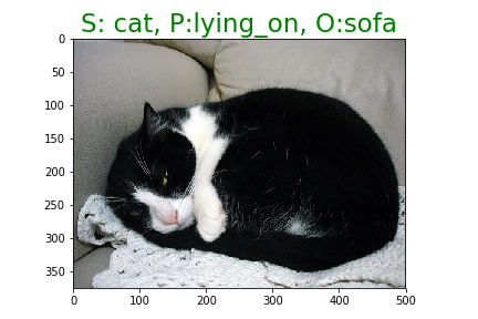
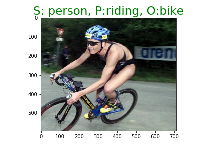
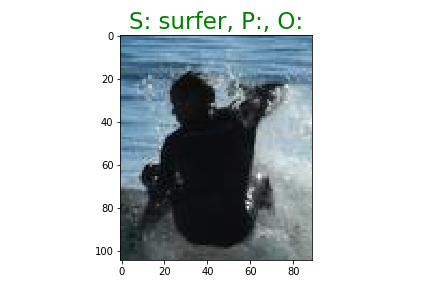
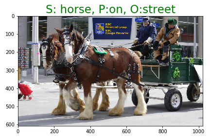
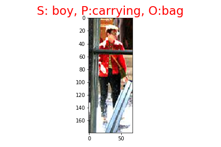
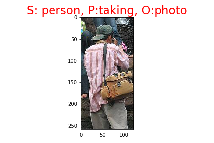
Figure 10: Correctly (title in green) and incorrectly (title in red) classified examples by MAS [1] on our Large-scale LLFL benchmark.

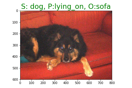
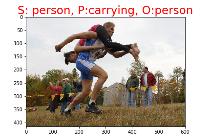
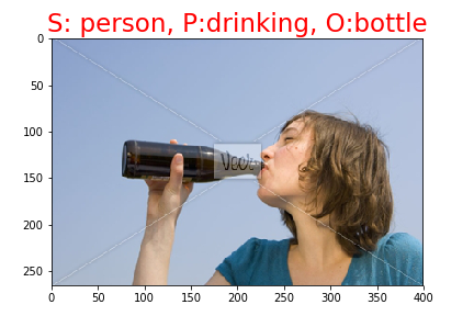
Figure 11: Correctly (title in green) and incorrectly (title in red) classified examples by Intelligent Synapses [30] on our Large-scale LLFL benchmark.

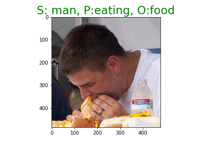
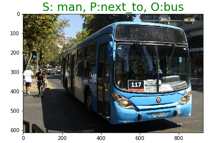
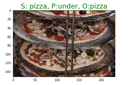
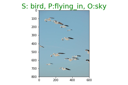
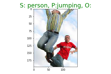
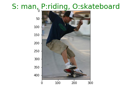
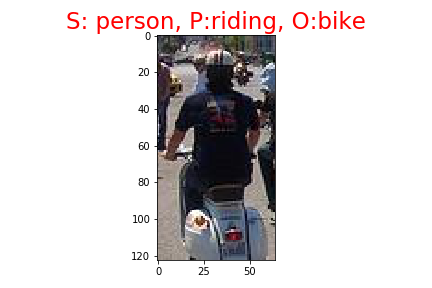
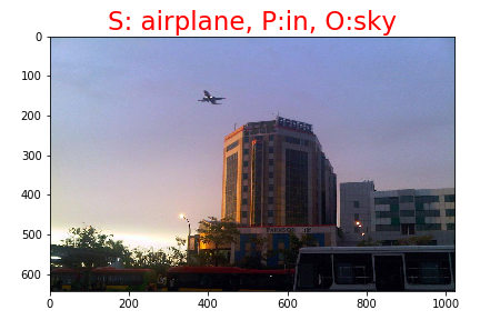
Figure 12: Correctly (title in green) and incorrectly (title in red) Classified examples by Finetuning on our Large-scale LLFL benchmark.

8 Mid-Scale benchmark Dendogram

Figure 13 shows the dendogram obtained from the agglomerative clustering performed in the word2vec space of the facts from the mid-scale dataset. The different colors indicate the different clusters. Each cluster later forms a task.

1. Cluster in magenta that mostly represents person actions and contains the person fact that is needed in the rest of that tasks.

2. Cluster in red resembles the second task and is mainly composed of facts of different objects.

3. Cluster in Cyan is the third cluster which contains facts describing humans holding or playing musical instruments.

4. Cluster in Green (last) is composed of the fact belonging to the green cluster that is composed of facts describing human interactions.

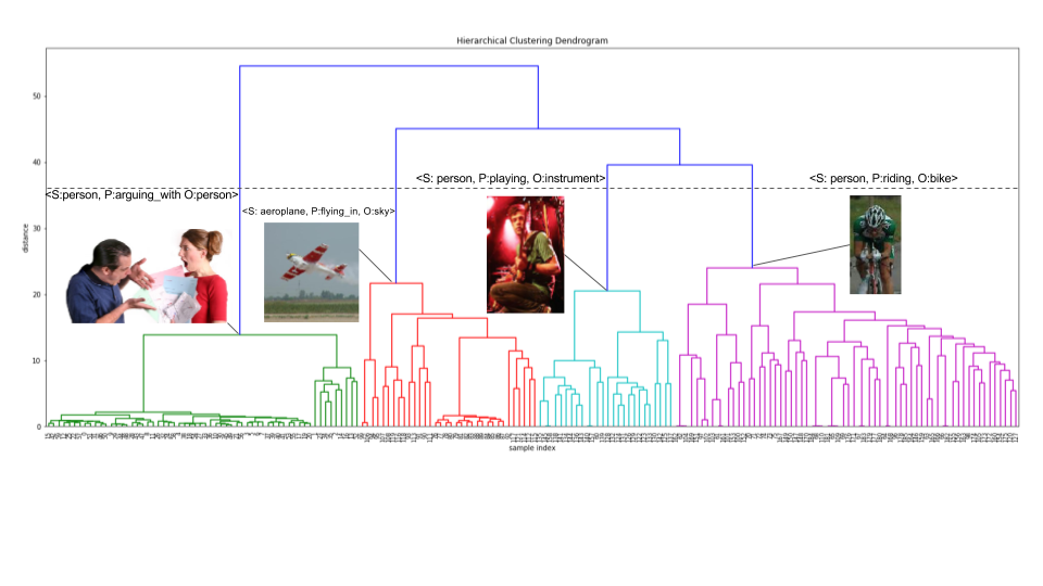
Figure 13: Lifelong Fact Learning for the Midscale dataset

References

- [1] Aljundi, R., Babiloni, F., Elhoseiny, M., Rohrbach, M., Tuytelaars, T.: Memory aware synapses: Learning what (not) to forget. In: ECCV (2018)
- [2] Aljundi, R., Chakravarty, P., Tuytelaars, T.: Expert gate: Lifelong learning with a network of experts. In: CVPR (2017)
- [3] Chao, W.L., Changpinyo, S., Gong, B., Sha, F.: An empirical study and analysis of generalized zero-shot learning for object recognition in the wild. In: European Conference on Computer Vision. pp. 52–68. Springer (2016)
- [4] Chaudhry, A., Dokania, P.K., Ajanthan, T., Torr, P.H.: Riemannian walk for incremental learning: Understanding forgetting and intransigence. In: International Conference on Machine Learning (2018)
- [5] Chen, X., Shrivastava, A., Gupta, A.: Neil: Extracting visual knowledge from web data. In: Computer Vision (ICCV), 2013 IEEE International Conference on. pp. 1409–1416. IEEE (2013)
- [6] Divvala, S.K., Farhadi, A., Guestrin, C.: Learning everything about anything: Webly-supervised visual concept learning. In: Proceedings of the IEEE Conference on Computer Vision and Pattern Recognition. pp. 3270–3277 (2014)
- [7] Elhoseiny, M., Cohen, S., Chang, W., Price, B.L., Elgammal, A.M.: Sherlock: Scalable fact learning in images. In: AAAI. pp. 4016–4024 (2017)
- [8] Fernando, C., Banarse, D., Blundell, C., Zwols, Y., Ha, D., Rusu, A.A., Pritzel, A., Wierstra, D.: Pathnet: Evolution channels gradient descent in super neural networks. arXiv preprint arXiv:1701.08734 (2017)
- [9] Gong, Y., Ke, Q., Isard, M., Lazebnik, S.: A multi-view embedding space for modeling internet images, tags, and their semantics. International journal of computer vision 106(2), 210–233 (2014)
- [10] He, K., Zhang, X., Ren, S., Sun, J.: Deep residual learning for image recognition. In: Proceedings of the IEEE conference on computer vision and pattern recognition. pp. 770–778 (2016)
- [11] Käding, C., Rodner, E., Freytag, A., Denzler, J.: Fine-tuning deep neural networks in continuous learning scenarios. In: Asian Conference on Computer Vision. pp. 588–605. Springer (2016)
- [12] Kirkpatrick, J., Pascanu, R., Rabinowitz, N., Veness, J., Desjardins, G., Rusu, A.A., Milan, K., Quan, J., Ramalho, T., Grabska-Barwinska, A., et al.: Overcoming catastrophic forgetting in neural networks. Proceedings of the national academy of sciences p. 201611835 (2017)
- [13] Kiros, R., Salakhutdinov, R., Zemel, R.S.: Unifying visual-semantic embeddings with multimodal neural language models. arXiv preprint arXiv:1411.2539 (2014)
- [14] Krizhevsky, A., Sutskever, I., Hinton, G.E.: Imagenet classification with deep convolutional neural networks. In: Advances in neural information processing systems. pp. 1097–1105 (2012)
- [15] Lee, S.W., Kim, J.H., Jun, J., Ha, J.W., Zhang, B.T.: Overcoming catastrophic forgetting by incremental moment matching. In: Advances in Neural Information Processing Systems. pp. 4652–4662 (2017)
- [16] Li, Z., Hoiem, D.: Learning without forgetting. In: European Conference on Computer Vision. pp. 614–629. Springer (2016)
- [17] Lomonaco, V., Maltoni, D.: Core50: a new dataset and benchmark for continuous object recognition. In: Conference on Robot Learning (2017)
- [18] Lopez-Paz, D., Ranzato, M.: Gradient episodic memory for continual learning. In: Advances in Neural Information Processing Systems (2017)
- [19] Mikolov, T., Sutskever, I., Chen, K., Corrado, G.S., Dean, J.: Distributed representations of words and phrases and their compositionality. In: Advances in neural information processing systems. pp. 3111–3119 (2013)
- [20] Mitchell, T.M., Cohen, W.W., Hruschka Jr, E.R., Talukdar, P.P., Betteridge, J., Carlson, A., Mishra, B.D., Gardner, M., Kisiel, B., Krishnamurthy, J., et al.: Never ending learning. In: AAAI. pp. 2302–2310 (2015)
- [21] Pasquale, G., Ciliberto, C., Rosasco, L., Natale, L.: Object identification from few examples by improving the invariance of a deep convolutional neural network. In: 2016 IEEE/RSJ International Conference on Intelligent Robots and Systems (IROS). pp. 4904–4911 (Oct 2016), http://ieeexplore.ieee.org/document/7759720/
- [22] Plummer, B.A., Mallya, A., Cervantes, C.M., Hockenmaier, J., Lazebnik, S.: Phrase localization and visual relationship detection with comprehensive image-language cues. In: Proceedings of the IEEE Conference on Computer Vision and Pattern Recognition. pp. 1928–1937 (2017)
- [23] Rebuffi, S.A., Kolesnikov, A., Lampert, C.H.: icarl: Incremental classifier and representation learning. arXiv preprint arXiv:1611.07725 (2016)
- [24] Romera-Paredes, B., Torr, P.: An embarrassingly simple approach to zero-shot learning. In: International Conference on Machine Learning. pp. 2152–2161 (2015)
- [25] Shmelkov, K., Schmid, C., Alahari, K.: Incremental learning of object detectors without catastrophic forgetting. In: The IEEE International Conference on Computer Vision (ICCV) (2017)
- [26] Simonyan, K., Zisserman, A.: Very deep convolutional networks for large-scale image recognition. arXiv preprint arXiv:1409.1556 (2014)
- [27] Thrun, S., O’Sullivan, J.: Clustering learning tasks and the selective cross-task transfer of knowledge. In: Learning to learn, pp. 235–257. Springer (1998)
- [28] Triki, A.R., Aljundi, R., Blaschko, M.B., Tuytelaars, T.: Encoder based lifelong learning. arXiv preprint arXiv:1704.01920 (2017)
- [29] Wang, Y.X., Ramanan, D., Hebert, M.: Growing a brain: Fine-tuning by increasing model capacity. In: IEEE Computer Society Conference on Computer Vision and Pattern Recognition (CVPR) (2017)
- [30] Zenke, F., Poole, B., Ganguli, S.: Continual learning through synaptic intelligence. In: Proceedings of the 34th International Conference on Machine Learning. vol. 70, pp. 3987–3995. PMLR (06–11 Aug 2017)
- [31] Zhang, J., Kalantidis, Y., Rohrbach, M., Paluri, M., Elgammal, A., Elhoseiny, M.: Large-scale visual relationship understanding. arXiv preprint arXiv:1804.10660 (2018)