Hyperbolic Deep Learning for Chinese Natural Language Understanding

Abstract

Recently hyperbolic geometry has proven to be effective in building embeddings that encode hierarchical and entailment information. This makes it particularly suited to modelling the complex asymmetrical relationships between Chinese characters and words. In this paper we first train a large scale hyperboloid skip-gram model on a Chinese corpus, then apply the character embeddings to a downstream hyperbolic Transformer model derived from the principles of gyrovector space for Poincare disk model. In our experiments the character-based Transformer outperformed its word-based Euclidean equivalent. To the best of our knowledge, this is the first time in Chinese NLP that a character-based model outperformed its word-based counterpart, allowing the circumvention of the challenging and domain-dependent task of Chinese Word Segmentation (CWS).

1 Introduction

Recent advances in deep learning have seen tremendous improvements in accuracy and scalability in all fields of application. Natural language processing (NLP), however, still faces many challenges, particularly in Chinese, where even word-segmentation proves to be a difficult and as-yet unscalable task.

Traditional neural network architectures employed to tackle NLP tasks are generally cast in the standard Euclidean geometry. While this setting is adequate for most deep learning tasks, where it has often allowed for the achievement of superhuman performance in certain areas (e.g. AlphaGo [35], ImageNet [36]), its performance in NLP has yet to reach the same levels. Recent research indicates that some of the problems NLP faces may be much more fundamental and mathematical in nature. It turns out that Euclidean geometry is unsuitable for properly dealing with data containing many hierarchical and asymmetrical relations. For instance, arbitrary trees, which are hierarchical data structures, cannot be properly embedded even in infinite-dimensional Euclidean space, yet even 2-dimensional hyperbolic space is “large” enough to embed arbitrary trees [1]. Additionally, hyperbolic geometries give rise to so-called “gyrovector spaces” [6] which are hyperbolic analogues of Euclidean vector spaces. Gyrovector spaces use gyrovector operations such as gyrovector addition (the hyperbolic analogue of vector addition) and scalar multiplication. Importantly, gyrovector addition is neither commutative nor associative, giving rise to a new mathematical way to capture asymmetrical relations in a mathematically sound framework.

In this paper, we will first discuss the problems inherent in Chinese Word-Segmentation (CWS). Then we give a primer on the background and fundamental concepts of hyperbolic geometry, and then describe both hyperbolic and Euclidean versions of word-embedding algorithms and the intent- classification algorithms which use these embeddings downstream. Lastly we discuss these results and conclude that hyperbolic geometry is a useful research direction, particularly in Chinese NLP, since in our experiments it appears that not only do hyperbolic versions of our algorithms outperform Euclidean ones, but they also appear to be able to circumvent the problem of CWS.

2 Chinese Word Segmentation

The state-of-the-art Chinese Word Segmentation (CWS) algorithms are bi-directional LTSMs [28]. CWS is an important yet challenging pre-processing step for Chinese NLP; this is because both characters and words carry semantic meaning, which are sometimes related, and sometimes unrelated. For example, related characters and words include

$$\begin{array}[]{| p{2cm} | p{2cm} | p{3.5cm} |}\hline\cr{Char}&\text{游}&\text{to swim (verb)}\\ \hline\cr{Char}&\text{泳}&\text{swimming (noun)}\\ \hline\cr{Word}&\text{游泳}&\text{to swim (noun/verb)}\\ \hline\cr\end{array}$$

$$\begin{array}[]{| p{2cm} | p{2cm} | p{3.5cm} |}\hline\cr{Char}&\text{微}&\text{micro}\\ \hline\cr{Char}&\text{波}&\text{wave}\\ \hline\cr{Char}&\text{爐}&\text{oven}\\ \hline\cr{Word}&\text{微波爐}&\text{microwave oven}\\ \hline\cr\end{array}$$

while unrelated characters and words include

$$\begin{array}[]{| p{2cm} | p{2cm} | p{3.5cm} |}\hline\cr{Char}&\text{香}&\text{fragrant}\\ \hline\cr{Char}&\text{港}&\text{harbor}\\ \hline\cr{Word}&\text{香港}&\text{Hong Kong}\\ \hline\cr\end{array}$$

and

$$\begin{array}[]{| p{2cm} | p{2cm} | p{3.5cm} |}\hline\cr{Char}&\text{幽}&\text{dark or quiet}\\ \hline\cr{Char}&\text{默}&\text{silently or secretly}\\ \hline\cr{Word}&\text{幽默}&\text{humor(ous)}\\ \hline\cr\end{array}$$

In addition, the same sentence can sometimes be segmented differently and still remain grammatically correct, making CWS dependent on context. For example:

$$\begin{array}[]{| l | l |}\hline\cr\text{結婚/的/和尚/没/結婚/的/學生。}&\text{A married monk and an unmarried student.}\\[2.5pt] \hline\cr\text{結婚/的/和/尚没/結婚/的/學生。}&\text{Married and unmarried students.}\\[2.5pt] \hline\cr\end{array}$$

Additionally, there exists different labelling standards - all equally logical - to the same sentence. For example:

$$\begin{array}[]{| p{6cm} | p{6cm} |}\hline\cr\text{案件/在/香港/區域/法院/審理。}&\text{The case is being heard in the }\\[2.5pt] \hline\cr\text{案件/在/香港/區域法院/審理。}&\text{District Court of Hong Kong SAR.}\\[2.5pt] \hline\cr\text{案件/在/香港區域法院/審理。}&\\[2.5pt] \hline\cr\end{array}$$

This makes the creation of a large scale CWS training corpus for deep learning-based segmentation engine difficult.

Lastly, domain specific vocabulary imposes extra scalability challenges, for example

$$\begin{array}[]{| p{3.5cm} | p{3.5cm} |}\hline\cr\text{量子引力}&\text{Quantum Gravity}\\ \hline\cr\text{林戴勝科}&\text{Wood Hoopoe}\\ \hline\cr\end{array}$$

A compromising solution is to train for high dimensional character embeddings in hopes of capturing the complex relationships between Chinese words and characters; however, downstream Euclidean models trained on Euclidean character embeddings have not been shown to match the performances of Euclidean models trained on word embeddings [37].

3 Hyperbolic Geometry

3.1 Riemannian Geometry

First we briefly describe Riemannian geometry concepts crucial for understanding our algorithms. Interested readers can refer to [5] for a more in-depth view of the topic. An $n$-dimensional manifold $\mathcal{M}$ is a smooth space that is locally flat, so that at each point $\mathbf{x}\in\mathcal{M}$, we associate a tangent space $T_{\mathbf{x}}\mathcal{M}$. A manifold is Riemannian if it admits an inner product at each point (also known as a metric) $g_{\mathbf{x}}:T_{\mathbf{x}}\mathcal{M}\to T_{\mathbf{x}}\mathcal{M}$. Due to the smoothness of the manifold, one can admit smooth parametrized curves on them $\gamma:\mathbb{R}\to\mathcal{M}$. For simplicity we assume the domain of the parametrized curves is $[0,1]$. The length of any parametrized curve $L$ is then determined by the metric: $L=\int_{0}^{1}\sqrt{g_{\gamma(t)}(\gamma^{\prime}(t),\gamma^{\prime}(t))}\,dt$. The minimum-length parametrized curve connecting two points on the manifold $\mathbf{x},\mathbf{y}\in\mathcal{M}$ is known as the geodesic between $\mathbf{x}$ and $\mathbf{y}$, and its length is known as the distance between points $\mathbf{x}$ and $\mathbf{y}$, denoted $d_{\mathcal{M}}(\mathbf{x},\mathbf{y})$.

It is often useful to transport vectors found in different tangent spaces in a parallel way to the same vector space so that we may operate on them using the same metric. This is known as parallel transport. Vectors in tangent spaces at any point can be parallel transported along geodesics to tangent spaces at other points such that they remain parallel (i.e. pointing in the same direction relative to the geodesic). This is done by breaking down the target vector into a linear combination of two orthogonal components: one pointing in the direction of the geodesic, and one pointing in the direction orthogonal to the geodesic. Parallel transport allows for more straight-forward addition of vectors found in different parts of the manifold. For a vector $\mathbf{v}\in T_{\mathbf{x}}\mathcal{M}$, we denote its parallel transport to the tangent space at another point $\mathbf{y}\in\mathcal{M}$ as $P_{\mathbf{x}\to\mathbf{y}}(\mathbf{v})$.

Often one needs a convenient way to map from tangent spaces back to the manifold and vice versa. To this end, we incorporate the exponential and logarithmic mappings, which are functions $\exp_{\mathbf{x}}:T_{\mathbf{x}}\mathcal{M}\to\mathcal{M}$ and $\log_{\mathbf{y}}:\mathcal{M}\to T_{\mathbf{y}}\mathcal{M}$. Essentially, for any tangent vector $\mathbf{v}\in T_{\mathbf{x}}\mathcal{M}$, we can map $\mathbf{v}$ to a point that is $\|\mathbf{v}\|$ away from $\mathbf{x}$ in the direction of $\mathbf{v}$ by using the exponential mapping. The logarithmic mapping is the local inverse of the exponential mapping.

As discussed in [9], the exponential and logarithmic mappings can be used to define hyperbolic versions of transformations in models of hyperbolic geometry whose tangent space at the origin resembles $\mathbb{R}^{n}$. If $f:\mathbb{R}^{n}\to\mathbb{R}^{m}$ is a Euclidean transformation, we can define a hyperbolic version of $f$, denoted $f^{\otimes}:\mathcal{M}^{n}\to\mathcal{M}^{m}$ that maps from an $n$-dimensional manifold $\mathcal{M}^{n}$ to its corresponding $m$-dimensional manifold $\mathcal{M}^{m}$ by

$$f^{\otimes}(\mathbf{x}) =\exp_{\mathbf{0}}(f(\log_{\mathbf{0}}(\mathbf{x})))$$

where $\exp_{\mathbf{0}}:T_{\mathbf{0}_{m}}\mathcal{M}^{m}\to\mathcal{M}^{m}$ and $\log_{\mathbf{0}}:\mathcal{M}^{n}\to T_{\mathbf{0}_{n}}\mathcal{M}^{n}$.

3.2 Analytic Hyperbolic Geometry

We want to establish an algebraic formalism for hyperbolic geometry that will help us perform operations in the same way that the vector-space structure of Euclidean geometry provides an algebraic formalism that allows the use of simple operations such as vector addition and scalar multiplication.

As detailed in [6], we can establish a non-associative algebraic formalism that allows for operations analogous to vector addition and scalar multiplication. This formalism is known as the theory of gyrovector spaces, and uses concepts from analytic hyperbolic geometry.

Essentially, a gyrovector space is like a vector space in that it is closed under its operations of scalar multiplication and gyrovector addition, and contains an identity element $\mathbf{0}$ and inverse elements $\ominus\mathbf{x}$. Unlike vector spaces, gyrovector addition, denoted $\oplus$, is not associative, but it is gyroassociative i.e. left-associative under the action of an automorphism known as a gyration. For any three gyrovectors $\mathbf{a},\mathbf{b},\mathbf{c}$, we have

$$\mathbf{a}\oplus(\mathbf{b}\oplus\mathbf{c}) =(\mathbf{a}\oplus\mathbf{b})\oplus\text{gyr}[\mathbf{a},\mathbf{b}]\mathbf{c}$$

where $\text{gyr}[\mathbf{a},\mathbf{b}]\mathbf{c}=\ominus(\mathbf{a}\oplus\mathbf{b})\oplus(\mathbf{a}\oplus(\mathbf{b}\oplus\mathbf{c}))$.

3.3 Models of Hyperbolic Geometry

In this paper we will concern ourselves chiefly with two $n$-dimensional models of hyperbolic geometry: the Poincaré ball, denoted $\mathbb{D}^{n}$ and the hyperboloid model, denoted $\mathbb{H}^{n}$. A detailed discussion of models of hyperbolic geometry and their relationships to one another can be found in [8].

3.3.1 The Poincaré Ball Model of Hyperbolic Geometry

The Poincaré ball of radius $c$ is a model of hyperbolic geometry defined by

$$\mathbb{D}^{n}_{c} =\{\mathbf{x}\in\mathbb{R}^{n}:\|\mathbf{x}\|<c\}.$$

its metric, denoted $g^{\mathbb{D}_{c}}$, is conformal to the Euclidean metric, denoted $g^{E}$, with a conformal factor $\lambda_{\mathbf{x}}^{c}$, i.e. $g_{\mathbf{x}}^{\mathbb{D}_{c}}=(\lambda_{\mathbf{x}}^{c})^{2}g^{E}$, where

$$\lambda_{\mathbf{x}}^{c}=\frac{2}{1-\frac{\|\mathbf{x}\|^{2}}{c^{2}}}$$

The Poincaré ball model of hyperbolic space forms a gyrovector space $(\mathbb{D}^{n}_{c},\oplus_{c},\otimes_{c})$ with gyrovector addition $\oplus$ and scalar multiplication $\otimes$ given by Möbius operations. As shown in [6], for $\mathbf{x},\mathbf{y}\in\mathbb{D}^{n}_{c}$, $r\in\mathbb{R}$, Möbius addition and scalar multiplication are given by

$$\mathbf{x}\oplus_{c}\mathbf{y} =\frac{(1+\frac{2}{c^{2}}\langle\mathbf{x},\mathbf{y}\rangle+\frac{1}{c^{2}}\|\mathbf{y}\|^{2})\mathbf{x}+(1-\frac{1}{c^{2}}\|\mathbf{x}\|^{2})\mathbf{y}}{1+\frac{2}{c^{2}}\langle\mathbf{x},\mathbf{y}\rangle+\frac{1}{c^{4}}\|\mathbf{x}\|^{2}\|\mathbf{y}\|^{2}}$$

$$r\otimes_{c}\mathbf{x} =c\tanh\left(r\tanh^{-1}\frac{\|\mathbf{x}\|}{c}\right)\frac{\mathbf{x}}{\|\mathbf{x}\|}$$

And its distance function is given by

$$d_{\mathbb{D}_{c}}(\mathbf{x},\mathbf{y})=2c\tanh^{-1}\left(\frac{1}{c}\|\ominus_{c}\mathbf{x}\oplus_{c}\mathbf{y}\|\right)$$

The exponential and logarithmic mappings for the Poincaré ball are derived in [9] and shown to be

$$\exp_{\mathbf{x}}^{c} =\mathbf{x}\oplus_{c}\left(\tanh\left(\frac{\lambda_{\mathbf{x}}^{c}\|\mathbf{v}\|}{2c}\right)\frac{c\mathbf{v}}{\|\mathbf{v}\|}\right)$$

$$\log_{\mathbf{x}}^{c}(y) =\frac{2c}{\lambda_{\mathbf{x}}^{c}}\tanh^{-1}\left(\frac{1}{c}\|\ominus_{c}\mathbf{x}\oplus_{c}\mathbf{y}\|\right)\frac{\ominus_{c}\mathbf{x}\oplus_{c}\mathbf{y}}{\|\ominus_{c}\mathbf{x}\oplus_{c}\mathbf{y}\|}$$

[9] also shows that scalar multiplication can be defined using these two mappings as $r\otimes_{c}\mathbf{x}=\exp_{\mathbf{0}}^{c}(r\log_{\mathbf{0}}^{c}(\mathbf{x}))$, and parallel transport of a tangent space vector at the origin $\mathbf{v}\in T_{\mathbf{0}}\mathbb{D}^{n}_{c}$ to any other tangent space $T_{\mathbf{x}}\mathbb{D}^{n}_{c}$ becomes

$$P_{\mathbf{0}\to\mathbf{x}}^{c}(\mathbf{v}) =\frac{\lambda_{\mathbf{0}}^{c}}{\lambda_{\mathbf{x}}^{c}}\mathbf{v}$$

Exponential and logarithmic mappings can also be used to define Möbius matrix-vector multiplication and bias translations:

$$M^{\otimes_{c}}(\mathbf{x}) =\begin{cases}c\tanh\left(\frac{\|M\mathbf{x}\|}{\|\mathbf{x}\|}\tanh^{-1}\left(\frac{\|\mathbf{x}\|}{c}\right)\right)\frac{M\mathbf{x}}{\|M\mathbf{x}\|}&\text{ if }M\mathbf{x}\neq\mathbf{0}\\ \mathbf{0}&\text{ if }M\mathbf{x}=\mathbf{0}\end{cases}$$

$$\mathbf{x}\oplus_{c}\mathbf{b} =\exp^{c}_{\mathbf{x}}(P^{c}_{\mathbf{0}\to\mathbf{x}}(\log^{c}_{\mathbf{0}}(\mathbf{b}))).$$

Finally, we note here that many of the formulae above become greatly simplified by setting the radius of the ball $c=1$, so we adopt this convention unless otherwise stated. We will, however, continue to use $\oplus_{c}$ to denote Möbius addition and $\otimes_{c}$ to denote Möbius scalar multiplication in order to draw attention to the fact that these operations are performed in the Poincaré ball model of hyperbolic geometry.

3.3.2 The Hyperboloid Model of Hyperbolic Geometry

A detailed discussion on the hyperboloid model can be found in [26]. The hyperboloid model is an $n$-dimensional manifold embedded in $(n+1)$-dimensional Minkowski space, denoted $\mathbb{R}^{(n,1)}$ which is the usual Euclidean $(n+1)$-dimensional vector space endowed with the Lorentzian inner product, which, for $\mathbf{x},\mathbf{y}\in\mathbb{R}^{(n,1)}$ is given by

$$\displaystyle\langle\mathbf{x},\mathbf{y}\rangle_{\mathcal{L}} =\sum_{i=1}^{n}x_{i}y_{i}-x_{n+1}y_{n+1}$$

and the Hyperboloid model is given by

$$\mathbb{H}^{n} =\{\mathbf{x}\in\mathbb{R}^{(n,1)}:\langle\mathbf{x},\mathbf{x}\rangle_{\mathcal{L}}=-1,x_{n+1}>0\}$$

and its metric is also given by the Lorentzian inner product: $g^{\mathbb{H}}_{\mathbf{x}}(\mathbf{u},\mathbf{v})=\langle\mathbf{u},\mathbf{v}\rangle_{\mathcal{L}}$. The distance between two points is given by

$$d_{\mathbb{H}}(\mathbf{u},\mathbf{v}) =\cosh^{-1}(-\langle\mathbf{u},\mathbf{v}\rangle_{\mathcal{L}})$$

If two points on the hyperboloid $\mathbf{x},\mathbf{y}\in\mathbb{H}^{n}$ are connected by a geodesic that points in the direction $\mathbf{v}$ of length $\|\mathbf{v}\|$, then we can consider a unit vector in the same direction $\hat{\mathbf{v}}$ and define the parallel transport of tangent space vectors $\mathbf{w}\in T_{\mathbf{x}}\mathbb{H}^{n}$ to the tangent space $T_{\mathbf{y}}\mathbb{H}^{n}$.

$$P_{\mathbf{x}\to\mathbf{y}}(\mathbf{w}) =\langle\mathbf{w},\mathbf{\hat{v}}\rangle_{\mathcal{L}}(\sinh(\|\mathbf{v}\|)\mathbf{x}+\cosh(\|\mathbf{v}\|)\mathbf{\hat{v}})+(\mathbf{w}-\langle\mathbf{w},\mathbf{\hat{v}}\rangle_{\mathcal{L}}\mathbf{\hat{v}})$$

Finally, we will often need to project vectors in the ambient Minkowski space onto the tangent spaces of the hyperboloid. To do this, suppose we have a point on the hyperboloid $\mathbf{x}\in\mathbb{H}^{n}$, and a vector in the ambient Minkowski space $\mathbf{v}\in\mathbb{R}^{(n,1)}$. We can project $\mathbf{v}$ onto the tangent space $T_{\mathbf{x}}\mathbb{H}^{n}$ using the following:

$$\text{proj}_{\mathbf{x}}(\mathbf{v}) =\mathbf{v}+\langle\mathbf{x},\mathbf{v}\rangle_{\mathcal{L}}\mathbf{x}.$$

4 Hyperbolic Neural Network Structures

4.1 Hyperboloid Char2Vec

The Euclidean skip-gram architecture found in [12] can be summarized as follows. Suppose we have a dictionary of words $\mathcal{V}$. Given a continuous stream of text $T=(w_{0},w_{1},...,w_{n})$, where $w_{i}\in\mathcal{V}$, skip-gram learns a vector representation in Euclidean space for each word by using it to predict surrounding words. Given a center word $w_{k}$, and $2\mu$ surrounding words (known as a context) given by $C=(w_{k-\mu},...,w_{k-1},w_{k+1},...,w_{k+\mu})$, the task is to predict $C$ from $w_{k}$. In order to train this model, we incorporate the negative sampling proposed in [13]. The center word and the context words are parametrized as two layers of a neural network, where the first layer represents the projection of the center word, and the output layer represents the context words. Suppose we wish to form embeddings of dimension $d$. Then we can parametrize these layers using matrices $A\in\mathbb{R}^{d\times|\mathcal{V}|}$ for the first layer and $B\in\mathbb{R}^{d\times|\mathcal{V}|}$. We index the columns of each matrix using the words from the dictionary $w_{i}\in\mathcal{V}$, i.e. $A_{w_{i}}$ and $B_{w_{i}}$. Suppose our center word is $w_{k}$. Let $w_{k+j}$ be some context word. Then negative sampling chooses $m$ random noise samples $\{w^{1},...,w^{m}\}$, and seeks to minimize the loss function given by

$$\displaystyle L_{w_{k},w_{k+j}}(A,B) =\prod_{i=0}^{m}p(y_{i}|w^{i},w_{k})$$

$$\propto\prod_{i=0}^{m}\sigma((-1)^{1-y_{i}}\langle A_{w_{k}},B_{w_{k+j}}\rangle)$$

where labels are given by $y_{0}=1$ and $y_{i}=0$ otherwise.

We wish to create word embeddings that capture both symmetric and asymmetrical relationships, and that efficiently model hierarchical relationships between words and characters. For this we turn to hyperbolic geometry. Since computing gradients on the hyperboloid model is easier than the Poincaré ball, [32][33] we follow [14] and use the hyperboloid model. To create a hyperboloid version of this loss function, [14] proposes replacing the above Euclidean dot product with the Lorentzian product with an additive shift:

$$\displaystyle L_{w_{k},w_{k+j}}(A,B) \propto\prod_{i=0}^{m}\sigma((-1)^{1-y_{i}}(\langle A_{w_{k}},B_{w_{k+j}}\rangle_{\mathcal{L}}+\theta))$$

We then optimize this loss function using Riemannian Stochastic Gradient Descent [31]. The details are given in the appendix.

4.2 Hyperbolic Transformer

Hyperboloid word embeddings are used downstream in a hyperbolic intent classification model. We use the Transformer architecture proposed in [21].

The core of the Euclidean version of Transformer is the operation called Scaled Dot Product attention. An input sequence is converted into three vectors, $Q,K\in\mathbb{R}^{d_{k}}$, and $V\in\mathbb{R}^{d_{v}}$ and the attention mechanism is then computed as follows:

$$\text{Attention}(Q,K,V)=\text{softmax}\left(\frac{QK^{T}}{\sqrt{d_{k}}}\right)V$$

The 3 vectors are split into $h$ heads via linear projections $W^{Q}_{i},W^{K}_{i}$ and $W^{V}_{i}$ with their results concatenated at the end, and then projected again by an output projection $W^{O}$. This allows the model to attend to multiple information subspaces simultaneously, resulting in better generalization. This is called Multi-head Attention, and is computed as follows: for $i=1,...,h$,

$$\text{head}_{i} =\text{Attention}(QW^{Q}_{i},KW^{K}_{i},VW^{V}_{i})$$

Multi-head $$=\text{concat}\left[\text{head}_{1},\ldots,\text{head}_{h}\right]W^{O}$$

The output of Multihead Attention is then fed into a fully connected layer. We stack $N$ layers of Transformer. To perform intent-classification, the final output of the Transformer is max pooled, fed to another fully connected feed-forward layer, and then finally softmaxed.

The Transformer itself does not capture information about the position of elements in the input sequence. In order to encode the positioning of these elements, we add a positional encoding to the input sequence of dimension $d$:

$$PE_{pos,2i}=\sin\left(\frac{pos}{10000^{\frac{2i}{d}}}\right), PE_{pos,2i+1}=\cos\left(\frac{pos}{10000^{\frac{2i}{d}}}\right).$$

The hyperbolic version of the Transformer architecture replaces Euclidean inputs with hyperbolic ones. Due to the simplicity of the expression for parallel transport of vectors in the Poincaré ball, we adopt this model of hyperbolic geometry. This means that our hyperboloid word-embeddings need to be transformed from the hyperboloid to the Poincaré model. This transformation is detailed in appendix A.

The positional encodings live in $\mathbb{R}^{n}$. Since this is equivalent to saying that they live in the tangent space at the origin of the Poincaré ball, we use the exponential mapping to map the encodings from this tangent space back down to the Poincaré ball, and then gyroadd the inputs and the positional encodings

$$\texttt{transformer\_input}=\texttt{input}\oplus_{c}\exp_{\mathbf{0}}^{c}(PE).$$

[22] suggests using a softmaxed hyperbolic distance function scaled by a temperature and translated by a bias, followed by a hyperbolic midpoint function, such as the Einstein midpoint function (see [6] ch. 6.20.1 Thm 6.87) to replace scaled dot product attention. We find, however, that leveraging parallel transport is a more numerically stable and successful paradigm to adopt in this case. We can parallel transport the query, key and value vectors to the origin using the logarithmic and exponential mappings, and then proceed to compute the scaled dot product attention using the standard Euclidean operations. This is viable because the tangent space at the origin of the Poincaré ball resembles $\mathbb{R}^{n}$.

To split our $n$-dimensional hyperbolic queries, keys and values into $m$ heads, each with dimension $h$ we need to use a single hyperbolic matrix multiplication first and then split into heads. For the input $\mathbf{x}\in\mathbb{D}^{n}_{c}$, we use a matrix $W\in\mathbb{R}^{3h\times n}$ to create a concatenated vector of heads, which we can then split:

$$W\otimes_{c}\mathbf{x} =\texttt{heads}=[\texttt{head}_{1},...,\texttt{head}_{m}]$$

These $\texttt{head}_{i}$ are then fed into the multihead attention. The result of each head must then be concatenated. However, straightforward concatenation is not a valid operation in hyperbolic space. Consequently, we must instead use hyperbolic matrix multiplication on each head individually and then gyroadd the results together at the end. So for $i=1,...,m$, we have

$$M_{i}\otimes_{c}\texttt{head}_{i} =\texttt{result}_{i}$$

$$\texttt{result}_{1}\oplus_{c}...\oplus_{c}\texttt{result}_{m} =\texttt{concatenated\_result}.$$

To modify the feed-forward neural network, we simply change it to a hyperbolic feed-forward neural network with two layers. For a hyperbolic neural network input $\mathbf{x}$, we have

$$M_{1}\otimes_{c}\mathbf{x}\oplus_{c}\mathbf{b}_{1} =\mathbf{h}$$

$$M_{2}\otimes_{c}\mathbf{h}\oplus_{c}\mathbf{b}_{2} =\hat{\mathbf{y}}$$

The output of the hyperbolic neural network is then max pooled and passed through a hyperbolic logistic regression algorithm in order to classify intents. Hyperbolic logistic regression is derived in [9] and detailed in the appendix.

5 Experiments

We have collected 16332 user utterances in the music domain. Each user utterance is a text-based voice command for an Alexa-like machine, with a labelled user intent.

Many of these utterances carry multiple commands such as query_song + increase_volume, thus inducing hierarchical relationships between composite intents and singular intents, warranting the use of hyperbolic machine learning. There are 125 intents in total. The list of intents can be found in the appendix section D.

We held out 15% of the dataset for evaluating intent classification accuracy.

Both Euclidean and hyperbolic character skip-gram embeddings are trained on a Chinese corpus of newspapers from Linguistic Data Consortium (LDC) of roughly 368 million characters [34].

For Euclidean Transformers, we used RMSProp optimisers [24] with a learning rate of 0.0001; hyperbolic Transformers were mostly optimised with RMSProp at a learning rate of 0.001, since most of the kernel matrices are Euclidean variables. The hyperbolic biases were optimised with Riemannian SGD [31] at a learning rate of 0.05. In all cases, Transformers consist of 3 multihead-attention layers, each of which splits its inputs into a total of 16 heads.

We trained 2 character-based Euclidean models, one 128-dimensional and the other 256-dimensional, while both character-based hyperbolic models are 100-dimensional. Both Euclidean models use a dropout of 20%. One of the hyperbolic models uses no dropout, and the other one uses a dropout of 30%.

To validate hyperbolic geometry’s suitability for modelling Chinese word-character relationships, we created another 256-dimensional Euclidean Transformer trained with word tokens instead of character tokens. The words were segmented with bi-directional LSTM + CRF [27] and a heavily music-domain-optimised post-processing dictionary. The word segmentation engine was trained on People’s Daily corpus [30], and the word-embeddings were also trained using Euclidean Skip-gram on the LDC data set.

All models were restarted once [29]; we observe an accuracy boost from restarts for all models.

	Intent Classification Accuracy	Cross-Entropy Loss
Eucl_TRF c2v 128D w/ 20% dropout	94.0%	0.4808
Eucl_TRF c2v 256D w/ 20% dropout	94.8%	0.4330
Eucl_TRF w2v 256D w/ 20% dropout	95.6%	0.1684
Hyp_TRF c2v 100D no dropout	96.2%	0.1729
Hyp_TRF c2v 100D w/ 30% dropout	96.9%	0.1226

Table 1: Intent Classification Accuracy and Cross-Entropy Loss for five different versions of the Transformer Model for intent classification. Despite being a lower-dimensional model, the hyperbolic Transformer outperforms its Euclidean counterpart.

6 Results

The results are shown in table 1. We first note that, as expected, the word-based Euclidean Transformer outperforms the character-based Euclidean Transformers. This is because training with word-based tokens allows the algorithm to model more complex and nuanced relationships between characters by simply identifying them as belonging to certain word tokens, which helps downstream to improve the accuracy of intent classification.

Of particular interest to us, however, is the marked improvement in accuracies of hyperbolic Transformers over their Euclidean counterparts. We believe that since words and characters form an obvious hierarchical relationship, and that words often have asymmetrical relationships between each other, that hyperbolic geometry is naturally better suited to encoding characters in a natural language understanding task, thus explaining these improved results.

Additionally, the fact that character-based hyperbolic intent classification (i.e. that makes use of character-based embeddings) still outperforms word-based Euclidean intent classification is a promising sign. It indicates that leveraging the power of hyperbolic representations of natural language can capture the hierarchical and asymmetrical relationships between words and characters well enough to circumvent the need for CWS altogether. This indeed is a promising research direction.

7 Conclusion

To the best of our knowledge, we have been the first to use hyperbolic embeddings in a downstream hyperbolic deep-learning task. Our results show that hyperbolic character-based intent-classification outperforms its character-based Euclidean counterpart, giving us confidence that hyperbolic embeddings and hyperbolic deep learning captures hierarchical and asymmetrical relationships in the Chinese language better than Euclidean embeddings and deep learning do. Additionally, we found that hyperbolic character-based intent-classification even outperforms Euclidean word-based intent-classification, which itself requires the use of state-of-the-art CWS. As we have discussed, CWS is a difficult and as-yet unscalable task, yet our results indicate that hyperbolic character-based deep-learning may be able to dispense with the need for this difficult task altogether. In our opinion, this indicates that hyperbolic deep learning merits further research, particularly in the realm of Chinese NLU.

Appendix

A. Relationship between Poincaré ball and Hyperboloid Model

The hyperboloid model can be visualized as the top part of a 2-sheet hyperboloid living in $\mathbb{R}^{3}$. Its plane of symmetry is the $xy$ plane. We can place a Poincaré disk of radius $c$ (usually $c=1$) on this plane of symmetry centered at the origin. We can map points from the Poincaré disk to the hyperboloid by projecting them from the disk to the hyperboloid with the vertex of the bottom part of the 2-sheet hyperboloid acting as the center of projection. This is shown in figure 1.

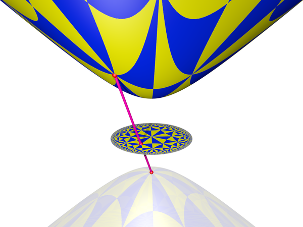
Figure 1: A hyperboloid model of hyperbolic space can be arrived at by placing a Poincaré disk at the plane of symmetry between a two sheet hyperboloid, and then projecting points from the Poincaré disk onto the upper sheet of a two sheet hyperboloid using the vertex of the lower sheet as the center of projection. This image is taken from [11].

This provides us with a simple way of determining a mapping and its inverse mapping from one model to the other. Suppose we wish to map from the hyerboloid model to the Poincaré disk. To do this, we simply define a projection function $\rho:\mathbb{H}^{n}\to\mathbb{D}^{n}$. Now suppose we choose a point $\mathbf{x}$ on the hyperboloid. Then $\mathbf{x}\in\mathbb{R}^{(n,1)}$ and $x_{n+1}>0$, and we can then define our projection of this point from the hyperboloid to the Poincaré disk as follows:

$$\rho(\mathbf{x})=\rho(x_{1},x_{2},...,x_{n},x_{n+1}) =\frac{1}{x_{n+1}+1}(x_{1},x_{2},...,x_{n})$$

and its inverse is given for any $\mathbf{y}\in\mathbb{D}^{n}$:

$$\rho^{-1}(\mathbf{y}) =\frac{2}{1-\|\mathbf{y}\|}\left(y_{1},y_{2},...,y_{n},\frac{1+\|\mathbf{y}\|^{2}}{2}\right)$$

In this way we can transform from one model to the other and back again at our convenience. This is useful as it allows us to leverage the advantages of both models where needed.

B. Riemannian Stochastic Gradient Descent of the Hyperboloid Model

This process is detailed in [14]. Gradients in Minkowski space $\mathbb{R}^{(n,1)}$ are taken with regard to the characteristics of the Lorentzian inner product. For a differentiable function $f:\mathbb{R}^{(n,1)}\to\mathbb{R}$, the gradient is given by

$$\nabla f=\left(\frac{\partial f}{\partial x_{0}},...,\frac{\partial f}{\partial x_{n-1}},-\frac{\partial f}{\partial x_{n}}\right)$$

These gradients can be projected into the tangent space $T_{\mathbf{x}}\mathbb{H}^{n}$ at a parameter point $\mathbf{x}$ to form Riemannian gradients. For the first layer parametrized by $A_{c}$, we have the following gradient equation for the log-likelihood

$$\displaystyle\nabla_{A_{c}}^{\mathbb{R}^{(n,1)}}\log L_{c,w_{0}}(A,B) =\sum_{i=0}^{k}(y_{i}-\sigma(\langle A_{c},B_{w_{i}}\rangle_{\mathcal{L}}+\theta))B_{w_{i}}$$

For the second layer, $B_{w}$, first consider the set consisting of the positive sample $w_{0}$ and all the negative samples $w_{1},...,w_{k}$ given by

$$\mathcal{S}_{c} =\{w_{0},w_{1},...,w_{k}\}.$$

Given any word $w\in\mathcal{V}$, let $N_{w,\mathcal{S}_{c}}$ be the number of times $w$ appears in $\mathcal{S}_{c}$, and let

$$y(w)=\begin{cases}1&\text{ if }w=w_{0}\\ 0&\text{ if }w\in\{w_{1},...,w_{k}\}\end{cases}$$

Then the gradient is given by

$$\nabla_{B_{w}}^{\mathbb{R}^{(n,1)}}\log L_{c,w_{0}}(A,B) =N_{w,\mathcal{S}_{c}}(y(w)-\sigma(\langle A_{c},B_{w_{i}}\rangle_{\mathcal{L}}+\theta))A_{c}$$

Next we project these gradients onto the tangent spaces of the hyperboloid. Recall that for a point $\mathbf{x}$ on the hyperboloid and a vector $\mathbf{v}$ in the ambient Minkowski space, we can project $\mathbf{v}$ onto the tangent space at $\mathbf{x}$ using

$$\text{proj}_{\mathbf{x}}(\mathbf{v}) =\mathbf{v}+\langle\mathbf{x},\mathbf{v}\rangle_{\mathcal{L}}\mathbf{x}$$

Then our projected gradients become

$$\nabla_{A_{c}}^{\mathbb{H}^{n}}\log L_{c,w_{0}}(A,B) =\text{proj}_{A_{c}}\left(\log L_{c,w_{0}}(A,B)\right)$$

$$\nabla_{B_{w}}^{\mathbb{H}^{n}}\log L_{c,w_{0}}(A,B) =\text{proj}_{B_{w}}\left(\log L_{c,w_{0}}(A,B)\right)$$

We then optimize the projected gradients using an exponential mapping on the negative gradient scaled by a learning factor $\eta$:

$$A_{c}^{\text{new}} =\exp_{A_{c}^{\text{old}}}(-\eta\nabla_{A_{c}^{\text{old}}}^{\mathbb{H}^{n}}\log L_{c,w_{0}}(A,B))$$

$$B_{w}^{\text{new}} =\exp_{B_{w}^{\text{old}}}(-\eta\nabla_{B_{w}^{\text{old}}}^{\mathbb{H}^{n}}\log L_{c,w_{0}}(A,B))$$

C. Hyperbolic Logistic Regression

[9] describes a version of hyperbolic multiclass logistic regression (hMLR) that is applicable to the Poincaré ball. However, since the models of hyperbolic space are all isometric to each other, it is not difficult to determine how to perform hMLR on any other model of hyperbolic space.

Suppose we have $K$ classes, $\{1,...,K\}$. Euclidean MLR learns a margin hyperplane for each class using softmax probabilities i.e. for all $k\in\{1,...,K\},b_{k}\in\mathbb{R}$ and $\mathbf{x},\mathbf{a}\in\mathbf{R}^{n}$, we have

$$p(y=k|\mathbf{x})\propto\exp(\langle\mathbf{a}_{k},\mathbf{x}\rangle-b_{k})$$

This can be formulated from the perspective of measuring distances to marginal hyperplanes. A hyperplane can be defined by a normal nonzero vector $\mathbf{a}\in\mathbb{R}^{n}$ and a scalar shift $b\in\mathbb{R}$:

$$H_{\mathbf{a},b} =\{\mathbf{x}\in\mathbb{R}^{n}:\langle\mathbf{a},\mathbf{x}\rangle-b=0\}$$

One can think of points in space $\mathbf{x}\in\mathbb{R}^{n}$ in relation to the hyperplane $H_{\mathbf{a},b}$ by examining the points in relation to the orientation of the hyperplane (as oriented by the normal vector $\mathbf{a}$) and its distance to the hyperplane (scaled by the magnitude of the normal vector $\|\mathbf{a}\|)$:

$$\langle\mathbf{a},\mathbf{x}\rangle-b=\text{sign}(\langle\mathbf{a},\mathbf{x}\rangle-b)\|\mathbf{a}\|d(\mathbf{x},H_{\mathbf{a},b})$$

We can substitute this into the equation for MLR:

$$p(y=k|\mathbf{x}) \propto\exp(\langle\mathbf{a}_{k},\mathbf{x}\rangle-b_{k})$$

$$=\exp(\text{sign}(\langle\mathbf{a}_{k},\mathbf{x}\rangle-b_{k})\|\mathbf{a}_{k}\|d(\mathbf{x},H_{\mathbf{a}_{k},b_{k}}))$$

We then reformulate by absorbing the bias term into the point, which creates a new definition for the hyperplane, where for $\mathbf{p}\in\mathbb{R}^{n}$

$$\tilde{H}_{\mathbf{a},\mathbf{p}} =\{\mathbf{x}\in\mathbb{R}^{n}:\langle-\mathbf{p}+\mathbf{x},\mathbf{a}\rangle=0\}$$

where $\tilde{H}_{\mathbf{a},\mathbf{p}}=H_{\mathbf{a},\langle\mathbf{a},\mathbf{p}\rangle}$. Then setting $b_{k}=\langle\mathbf{a}_{k},\mathbf{p}_{k}\rangle$, we can rewrite MLR

$$p(y=k|\mathbf{x}) \propto\exp(\text{sign}(\langle\mathbf{a}_{k},\mathbf{x}\rangle-b_{k})\|\mathbf{a}_{k}\|d(\mathbf{x},H_{\mathbf{a}_{k},\langle\mathbf{a}_{k},\mathbf{p}_{k}\rangle}))$$

$$=\exp(\text{sign}(\langle\mathbf{a}_{k},\mathbf{x}\rangle-\langle\mathbf{a}_{k},\mathbf{p}_{k}\rangle)\|\mathbf{a}_{k}\|d(\mathbf{x},H_{\mathbf{a}_{k},b_{k}}))$$

$$=\exp(\text{sign}(\langle-\mathbf{p}_{k}+\mathbf{x},\mathbf{a}_{k}\rangle)\|\mathbf{a}_{k}\|d(\mathbf{x},\tilde{H}_{\mathbf{a}_{k},\mathbf{p}_{k}}))$$

which we can then convert to a hyperbolic version in a manifold $\mathcal{M}$ with metric $g$:

$$\tilde{H}^{\mathcal{M}}_{\mathbf{a},\mathbf{p}} =\{\mathbf{x}\in\mathcal{M}:\langle\ominus\mathbf{p}\oplus\mathbf{x},\mathbf{a}\rangle=0\}$$

$$p(y=k|\mathbf{x}) \propto\exp\left(\text{sign}(\langle\ominus\mathbf{p}_{k}\oplus\mathbf{x},\mathbf{a}_{k}\rangle)\sqrt{g_{\mathbf{p}_{k}}(\mathbf{a}_{k},\mathbf{a}_{k})}d_{\mathcal{M}}(\mathbf{x},\tilde{H}_{\mathbf{a}_{k},\mathbf{p}_{k}})\right)$$

In particular, for a Poincaré ball of dimension $n$ and radius $c$, denoted $\mathbb{D}^{n}_{c}$:

$$p(y=k|\mathbf{x}) \propto\exp\left(c\lambda^{c}_{\mathbf{p}_{k}}\|\mathbf{a}_{k}\|\sinh^{-1}\left(\frac{2\langle\ominus\mathbf{p}_{k}\oplus\mathbf{x},\mathbf{a}_{k}\rangle}{c(1-\frac{1}{c^{2}}\|\ominus\mathbf{p}_{k}\oplus\mathbf{x}\|^{2})\|\mathbf{a}_{k}\|}\right)\right)$$

and this can be optimized using Riemannian optimization.

D. List of Intent Types

add_playing_song_to_blacklist
add_playing_song_to_blacklist+query_song_hit+play_song
add_preference
add_preference+play_song
add_preference+query_song_hit+play_song
add_to_blacklist
add_to_favourite
add_to_favourite+play_song
add_to_favourite+sort_playlist
add_to_favourite+sort_playlist+play_song
add_to_playing_list
add_to_playing_list+play_song
add_to_playing_list+sort_playlist
add_to_playing_list_next
add_to_playlist
add_to_playlist+play_song
add_to_playlist+sort_playlist
add_to_playlist+sort_playlist+play_song
create_playlist
create_playlist+play_song
create_playlist_from_current
destroy_playlist
fastbackward_song
fastforward_song
list_favourite
list_playing_list
list_playlist
loop_play_album
loop_play_playing_list
loop_play_playlist
loop_play_song
move_from_playlist
move_from_playlist+play_song
music_pause
next_song
next_song+loop_play_song
others
pause_song
pause_song+play_song
play_random
play_song
play_song_get_album
play_song_get_album+loop_play_album
play_song_get_album+loop_play_playing_list
play_song_get_artist+add_to_blacklist
play_song_get_artist+loop_play_playing_list
play_song_get_genre+add_to_blacklist
play_song_get_song
play_song_get_song+add_to_blacklist
play_song_get_song+add_to_playlist
play_song_get_song+query_song
previous_song
query_favourite+play_song
query_hit_song+add_to_favourite
query_lyric
query_lyric+add_to_favourite
query_lyric+add_to_playing_list
query_lyric+add_to_playlist
query_lyric+play_song
query_lyric_get_mood
query_playlist
query_playlist+play_song
query_preference
query_preference+add_to_favourite
query_preference+add_to_playing_list
query_preference+add_to_playlist
query_preference+play_song
query_song
query_song+add_to_blacklist
query_song+add_to_favourite
query_song+add_to_favourite+play_song
query_song+add_to_playing_list
query_song+add_to_playing_list_next+query_song
query_song+add_to_playlist
query_song+add_to_playlist+loop_play_playlist
query_song+clock_alarm_set
query_song+loop_play_playing_list
query_song+loop_play_song
query_song+play
query_song+play_song
query_song+play_song+add_to_playlist
query_song+play_song+query_song+play_song+play_song
query_song+vol_max+play_song
query_song_get_album
query_song_get_artist
query_song_get_genre
query_song_hit
query_song_hit+add_to_favourite
query_song_hit+add_to_playing_list
query_song_hit+add_to_playlist
query_song_hit+create_playlist
query_song_hit+play_song
query_song_hit+play_song+stop_song_after
query_song_hit+query_song+play_song
query_song_latest
query_song_latest+play_song
query_song_latest_album+play_song
query_song_playlist
query_song_preference+play_song
query_song_random
query_song_random+add_to_favourite
query_song_random+add_to_playing_list
query_song_random+add_to_playlist
query_song_random+clock_alarm_set
query_song_random+play_song
query_song_random+play_song+add_to_favourite
remove_from_blacklist
remove_from_playing_list
remove_from_playlist
remove_playlist
remove_preference
replace_song_in_playlist
replace_song_in_playlist+play_song
reset_playing_list
reset_playlist
resume_song
sort_playing_list
sort_playlist
stop_song
stop_song_after
vol_decrease
vol_increase
vol_max
vol_min
vol_set

References

- [1] De Sa, Christopher, Gu, Albert, Ré, Christopher, Sala, Frederic (2018) Representation Tradeoffs for Hyperbolic Embeddings accessed on 2018-10-16 at https://arxiv.org/abs/1804.03329
- [2] Joyce, David E. (1996) Euclid’s Elements accessed on 2018-10-23 at https://mathcs.clarku.edu/~djoyce/java/elements/elements.html
- [3] Weisstein, Eric W. Gaussian Curvature From MathWorld – a Wolfram Web Resource accessed on 25-10-2018 at http://mathworld.wolfram.com/GaussianCurvature.html
- [4] Weisstein, Eric W. Great Circle From MathWorld – a Wolfram Web Resource accessed on 25-10-2018 at http://mathworld.wolfram.com/GreatCircle.html
- [5] Petersen, Peter, (2006) Riemannian Geometry accessed on 29-10-2018 at http://math.ecnu.edu.cn/~lfzhou/seminar/[Petersen_P.]_Riemannian_geometry.pdf
- [6] Ungar, Abraham A. (2005) Analytic Hyperbolic Geometry
- [7] Lang, Serge, (1987) Linear Algebra Third Edition, accessed on 31-10-2018 at https://fit.mta.edu.vn/files/DanhSach/serge-lang-linear-algebra.pdf
- [8] Cannon, James W., Floyd, Willian J., Kenyon, Richard, Parry, Walter R. (1997) Hyperbolic Geometry from Flavors of Geometry vol. 31 accessed on 31-10-2018 at http://library.msri.org/books/Book31/files/cannon.pdf
- [9] Ganea, Octavian-Eugen, Bécigneul, Gary (2018) Hyperbolic Neural Networks accessed on 31-10-2018 at https://arxiv.org/pdf/1805.09112.pdf
- [10] Mendel, M. B., van Galder, P.H.A.J.M. (2017) Visualizing and Gauging Collision Risk accessed on 01-11-2018 at https://www.researchgate.net/publication/313803470_Visualizing_and_gauging_collision_risk
- [11] von Gagern, Martin F. (2014) Creation of Hyperbolic Ornaments - Algorithmic and Interactive Methods accessed on 01-11-2018 at http://mediatum.ub.tum.de/?id=1210572
- [12] Mikolov, Tomas, Chen, Kai, Corrado, Greg, Dean, Jeffrey, (2013) Efficient Estimation of Word Representations in Vector Space accessed on 05-11-2018 at https://arxiv.org/pdf/1301.3781.pdf
- [13] Mikolov, Tomas, Sutskever, Ilya, Chen, Kai, Corrado, Greg, Dean, Jeffrey (2013) Distributed Representations of Words and Phrases and their Compositionality accessed on 06-11-2018 at https://arxiv.org/pdf/1310.4546.pdf
- [14] Leimeister, Matthias, Wilson, Benjamin J. (2018) Skip-gram Word Embeddings in Hyperbolic Space accessed on 06-11-2018 at https://arxiv.org/pdf/1809.01498.pdf
- [15] Cho, Kyunghyun, van Merriënboer, Bart, Gulcehre, Caglar, Bahdanau, Dzimitry, Bougares, Fethi, Schwenk, Holger, Bengio, Yoshua (2014) Learning Phrase Representations using RNN Encoder-Decoder for Statistical Machine Translation accessed on 08-11-2018 at https://arxiv.org/pdf/1406.1078.pdf
- [16] Pennington, Jeffrey, Socher, Richard, Manning, Christopher D. (2014) GloVE: Global Vectors for Word Representation accessed on 26-11-2018 at https://www.aclweb.org/anthology/D14-1162
- [17] Tifrea, Alexandru, Bécigneul, Gary, Ganea, Octavian-Eugen, (2018) Poincaré GLOVE: Hyperbolic Word Embeddings accessed on 27-11-2018 at https://arxiv.org/pdf/1810.06546.pdf
- [18] Costa, S. I. R., Santos, S. A., Strapasson, J. E. (2014) Fisher Information Distance: A Geometrical Reading accessed on 29-11-2018 at https://arxiv.org/pdf/1210.2354.pdf
- [19] Cover, Thomas M., Thomas, Joy A., (1991) Elements of Information Theory 2nd edition, accessed on 03-12-2018 at http://www.cs-114.org/wp-content/uploads/2015/01/Elements_of_Information_Theory_Elements.pdf
- [20] Haber, Howard E. (2011) The Volume and Surface Area of an -dimensional hypersphere presented as lecture notes for the class PHYS116A in Winter 2011 at the University of California, Santa Cruz, accessed on 04-12-2018 at http://scipp.ucsc.edu/~haber/ph116A/volume_11.pdf
- [21] Vaswani, Ashish, Shazeer, Noam, Parmar, Niki, Uszkoreit, Jakob, Jones, Llion, Gomez, Aidan N., Kaiser, Lukasz, Polosukhin, illia (2017) Attention is All You Need, accessed on 2018-06-06 at https://arxiv.org/pdf/1706.03762.pdf
- [22] Gulcehre, Caglar, Denil, Misha, Malinowski, Mateusz, Razavi, Ali, Pascanu, Razvan, Herman, Karl Moritz, Battaglia, Peter, Bapst, Victor, Raposo, David, Santoro, Adam, de Freitas, Nando, (2018) Hyperbolic Attention Networks accessed on 2018-12-04 at https://arxiv.org/pdf/1805.09786.pdf
- [23] Bécignuel, Gary, Ganea, Octavian-Eugen (2018) Riemannian Adaptive Optimization Methods accessed on 07-12-2018 at https://arxiv.org/pdf/1810.00760.pdf
- [24] Hinton, Geoffrey, Srivastava, Nitish, Swersky, Kevin, Lecture 6a of the course “Neural Networks for Machine Learning, Overview of mini-batch gradient descent accessed on 07-12-2018 at http://www.cs.toronto.edu/~tijmen/csc321/slides/lecture_slides_lec6.pdf
- [25] Huang, Zhiheng, Xu, Wei, Yu, Kai (2015) Bidirectional LSTM-CRF Models for Sequence Tagging accessed on 10-12-2018 at https://arxiv.org/pdf/1508.01991.pdf
- [26] Reynolds, William F., (1993) Hyperbolic Geometry on a Hyperboloid accessed on 29-11-2018 at https://people.ucsc.edu/~rmont/classes/ClassicalGeometry/2015/LectureNotes/Reyolds_onaHyperboloid.pdf
- [27] Chen, Xinchi, Qiu, Xipeng, Zhu, Chenxi, Liu, Pengfei, Huang, Xuanjing, (2015) Long Short-Term Memory Neural Networks for Chinese Word Segmentation accessed on 11-12-2018 at http://aclweb.org/anthology/D15-1141
- [28] Ma, Ji, Ganchev, Kuzman, Weiss, David, (2018) State-of-the-Art Chinese Word Segmentation with Bi-LTSMs accessed on 11-12-2018 at https://arxiv.org/pdf/1808.06511.pdf
- [29] Loshchilov, Ilya, Hutter, Frank (2017) SGDR: Stochastic Gradient Descent with Warm Restarts accessed on 11-12-2018 at https://arxiv.org/pdf/1608.03983.pdf
- [30] Yu, Shiwen et al (2001) Guideline of People’s Daily Corpus Annotation Technical Report, Beijing University.
- [31] Bonnabel, Silvere, (2011) Stochastic Gradient Descent on Riemannian Manifolds accessed on 11-12-2018 at https://arxiv.org/pdf/1111.5280.pdf
- [32] Wilson, Benjamin, Leimeister, Matthias, (2018) Gradient Descent in Hyperbolic Space accessed on 11-12-2018 at https://arxiv.org/pdf/1805.08207.pdf
- [33] Nickel, Maximillian, Kiela, Douwe (2018) Learning Continuous Hierarchies in the Lorentz Model of Hyperbolic Space accessed on 11-12-2018 at https://arxiv.org/pdf/1806.03417.pdf
- [34] Linguistic Data Consortium, available at https://www.ldc.upenn.edu/
- [35] Deepmind Research, Alpha Go available at https://deepmind.com/research/alphago/
- [36] ImageNet, available at http://www.image-net.org/
- [37] Chen, Xinxiong, Xu, Lei, Liu, Zhiyuan, Sun, Maosong, Luan, Huanbo, (2015) Joint Learning of Character and Word Embeddings accessed on 11-12-2018 at http://nlp.csai.tsinghua.edu.cn/~lzy/publications/ijcai2015_character.pdf