Investigation of Cyclic Liquefaction with Discrete Element Simulations

Abstract

A discrete element (DEM) assembly of virtual particles is calibrated to approximate the behavior of a natural sand in undrained loading. The particles are octahedral, bumpy clusters of spheres which are compacted into assemblies of different densities. The contact model is a Jäger generalization of the Hertz contact, yielding a small-strain shear modulus that is proportional to the square root of confining stress. Simulations of triaxial extension and compression loading conditions and of simple shear produce behaviors that are similar to sand. Undrained cyclic shearing simulations are performed with non-uniform amplitudes of shearing pulses and with 24 irregular seismic shearing sequences. A methodology is proposed for quantifying the severities of such irregular shearing records, allowing the 24 sequences to be ranked in severity. The relative severities of the 24 seismic sequences show an anomalous dependence on sampling density. Four scalar measures are proposed for predicting the severity of a particular loading sequence. A stress-based scalar measure shows superior efficiency in predicting initial liquefaction and pore pressure rise.

Liquefaction, discrete element method, contact mechanics, simulation, undrained loading.

1 Introduction

Cyclic liquefaction is commonly thought to develop from the micro-scale jostling of particles during repeated load reversals or rotations of the principal stresses, causing a progressive rearrangement of the particles and a tendency of the soil to contract. This tendency, under undrained conditions, produces positive pore pressure, which leads to a reduction in effective stress and a diminished capacity of the particles to sustain load. In the context of understanding soil behavior at the micro-scale, rather than at the meta-scale of continuum constitutive approaches, the micro-level basis of liquefaction was confirmed in the particle-scale discrete element (DEM) simulations of Hakuno:1988a and Dobry:1992a. Over twenty years old, these simulations of two-dimensional arrays of disks and spheres may seem inelegant by current standards, but they gave convincing demonstration of a micro-scale origin of cyclic loading behavior: pore pressure rise concurrent with loading and a degradation of the shear modulus with increasing strain magnitude. In a later series of two-dimensional simulations, Ashmawy:2003a produced realistic liquefaction curves, giving the relationship between cyclic stress amplitude and the number of cycles to failure. Other simulations have shown that the load-bearing capacity of a granular material is diminished during repeated loading, reducing the number of inter-particle contacts, leading to pore pressure rise under undrained conditions, and altering the fabric anisotropy [Ng and Dobry (1994), Sitharam (2003), Sazzad and Suzuki (2010)]. Recently, the interplay of pore fluid and grains has been simulated by coupling DEM with discretized Navier-Stokes models, permitting the simulation of entire soil strata to track the progression of larger-scale phenomena such as lateral spreading and the upward migration of water during ground shaking.

The current work uses the Discrete Element Method (DEM) to explore the cyclic liquefaction behavior of a target sand (Nevada Sand), attempting a modest fidelity to its measured, laboratory behavior. After showing that the model captures many aspects of this sand’s behavior, we use the model to simulate conditions that can occur in the field but would be difficult to manage in a laboratory setting. We arrive at a predictive measure of loading conditions conducive to liquefaction.

The DEM simulations in this study used the open source OVAL code [Kuhn (2002)] and are element tests, in which small assemblies of “particles in a box” undergo various deformation sequences. The purpose is to explore the material behavior of a simulated soil element — representing an idealized material point in a soil continuum or an integration point in a finite element model — rather than to study a larger boundary value problem (e.g., a footing foundation or an entire soil column, as with ElShamy:2012,ElShamy:2005a). Figure 1 shows an assembly of 6400 particles, representing a small soil element of size $18\times 12\times 12\,D_{50}$ (about $3\times 2\times 2$mm): large enough to capture the average material behavior but sufficiently small to prevent meso-scale localization, such as shear bands, or the macro-scale non-uniformities produced by boundary conditions (footings, excavations, etc.).

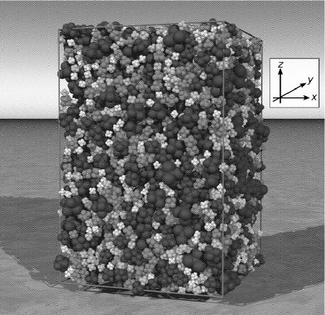
Figure 1: Discrete element (DEM) assembly of 6400 particles.

In the study, we exploit certain advantages of DEM simulations for exploring material behavior. Once a DEM assembly is created, the same assembly can be reused with loading sequences of almost unlimited variety, all beginning from precisely the same particle arrangement, during which all Cartesian components of stress and strain are accessible. DEM element tests also permit loading sequences with arbitrary control of any six components of the stress and strain rates or of their linear combinations—loading conditions that would require different testing apparatus in a physical laboratory. The average stress within an assembly is computed from the inter-granular contact forces, so that the computed stresses are inherently effective stresses.

The following section presents details of the DEM model, focusing on refinements to current models. This section is followed by presentations of the model’s monotonic and cyclic loading behaviors. The cyclic response is explored for level-ground conditions of cyclic simple shear in which shear stress is applied in three types of sequences: uniform-amplitude loading, non-uniform amplitude sequences, and realistic seismic loading sequences. These simulations are used to evaluate proposed “severity measures” for predicting the onset of liquefaction.

2 Granular Assembly

DEM assemblies (Fig. 1) were constructed with the goal of approximating the behavior of Nevada Sand, a standard poorly graded sand (SP) used in laboratory and centrifuge testing programs, including the VELACS program [Arulanandan and Scott (1993), Arulmoli et al. (1992), Cho et al. (2006), Duku et al. (2008)]. A DEM model can be customized by adjusting several characteristics, including (1) particle size and size distribution, (2) particle shape, (3) compaction procedure, (4) the contact force-displacement relation, and (5) the contact friction coefficient. At the outset, we recognized that a DEM model is unlikely to reproduce all behaviors of a targeted soil, and we set modest goals relative to Nevada Sand: similarities in particle size distribution, range of void ratios, small-strain stiffness, and critical state friction angle.

Attaining the desired median particle size $D_{50}=0.165$mm is a simple matter of scaling the DEM particles, but fashioning the size distribution involves some compromise, since computation time is favored by a smaller range of particle sizes. For this reason, particle sizes were selected to fit the central portion of the particle size distribution of Nevada Sand (Fig. 2), neglecting the smallest and largest 3.5% of sizes.

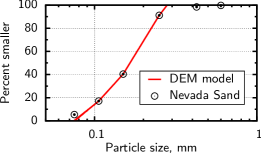
Figure 2: Particle size distributions.

An assembly of spheres can not adequately represent a natural sand: sphere packings have a narrow range of void ratios (typically $e=0.55$ to 0.73 for glass ballotini, Zettler:2000a); a sphere can touch a neighboring sphere only at a single contact; and sphere assemblies have relatively low strength (a friction angle $\phi$ of about 20^∘, Cho:2006a). To achieve more realistic simulations, we chose a bumpy, compound cluster shape having a large central sphere with six embedded “satellite” spheres in an octahedral arrangement (Fig. 3). Besides its computational advantages, the shape has sufficient non-roundness to produce a large range of initial densities, and the basic shape can be modified to attain a targeted range of densities (i.e., one can modify the relative radii of the single central sphere and the outer satellite spheres as well as the relative protrusions of the outer spheres). As guidance, we used the work of Cho:2006a, who developed correlations between a sand’s particle shape and its strength and density range. Salot:2009a studied the effect of DEM particle shape and contact friction on density and strength, and they developed a procedure for calibrating a DEM assembly to approximate the behavior of a targeted sand. With this guidance and considerable trial and error, we arrived at a shape that produced a realistic strength and range of void ratios, as described below. This shape has a ratio of central-to-satellite sphere radii of 0.75, and the satellite spheres were centered at octahedral points located 0.925 of the radius of the inner sphere from its center (Fig. 3).

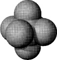
Figure 3: Particle shape: a bumpy octahedral cluster of spheres.

In a laboratory setting, sand can be conditioned, placed, and compacted in various ways to produce a desired density and fabric. Because many of these laboratory procedures can not yet be simulated, we used a simpler computational procedure that produces assemblies with a similar range of densities as Nevada Sand and with a modest fabric anisotropy, as would be expected with a laboratory pluviation procedure. To start, the 6400 particles were sparsely and randomly arranged within a spatial cell surrounded by periodic boundaries. In the absence of gravity and with a reduced inter-particle friction coefficient ($\mu=0.30$), the assembly was anisotropically (uniaxially) compacted by slowly reducing its height but with no lateral strain. The initially sparse arrangement with zero stress would eventually “seize” when a loose, yet load-bearing, fabric had formed. A series of fourteen progressively denser assemblies were created by repeatedly assigning random velocities to particles of the previous assembly (simulating a disturbed or vibrated state) and then further reducing the assembly height until the newer specimen had seized again. The fifteen specimens had void ratios in the range $e_{\text{loosest}}$ to $e_{\text{densest}}$ of 0.850 to 0.525, a range that is similar to that of Nevada Sand obtained with standard ASTM procedures. Although the authors do not contend that virtual specimens with a range $e_{\text{loosest}}$ to $e_{\text{densest}}$ correspond to the range $e_{\text{max}}$ to $e_{\text{min}}$ attained with ASTM procedures, some auxiliary evidence does support a similarity in the two ranges. Attempting to simulate glass ballotini, the same DEM procedure was applied to create assemblies of spherical particles having a narrow range of diameters. The simulated compaction procedure results in assemblies with the range $e_{\text{loosest}}$ to $e_{\text{densest}}$ of 0.750 to 0.549, which compares favorably with ranges $e_{\text{max}}$ to $e_{\text{min}}$ that have been reported for ballotini prepared with the ASTM procedures, about 0.73 to 0.58 [Zettler et al. (2000)].

Having created fifteen assemblies with this anisotropic compaction scheme, the friction coefficient $\mu$ was raised to $0.60$ and each assembly was isotropically consolidated to a mean effective stress of 10kPa. This step simulates the isotropic consolidation of a pluviated sample, as in standard triaxial testing, and leaves the sample with a small initial anisotropy (a Satake fabric anisotropy $F_{zz}/F_{xx}=1.08$). Most results in the paper involve a further isotropic consolidation to the higher stress of 80kPa, so that results can be compared with the Nevada Sand tests of Arulmoli1992a. In short, the preparation initially created assemblies with an anisotropic fabric at low stress, followed by isotropic consolidation to a mean effective stress of 10kPa or higher.

The small-strain behavior of a DEM assembly is sensitive to the particular force-displacement model of the contacts. During cyclic loading of a sand, the mean effective stress $p$ can be progressively reduced to nearly zero, and further cyclic loading causes $p$ to rise and fall across a broad range of values. We believe that the proper simulation of liquefaction requires a contact model that appropriately reflects a sand’s small-strain material behavior over a range of $p$. As a minimum, the relationship between small-strain bulk shear modulus $G_{\text{max}}$ and mean effective stress $p$ should comport with that of sand. The modulus $G_{\text{max}}$ of sands is usually found to vary in proportion to $p^{\beta}$, where exponent $\beta$ is in the range 0.4–0.6, depending on particle shape [Cho et al. (2006)], particle size gradation [Wichtmann and Triantafyllidis (2009)], surface roughness [Santamarina and Cascante (1998)], and pre-load conditioning. A $\beta$ of 0.5 is commonly used in geotechnical practice and for correlations among $G_{\text{max}}$, $e$, and $p$ [Hardin (1978)]. A exponent of 0.5 also fits the data for Nevada Sand [Arulmoli et al. (1992)] and was the targeted exponent in our study.

From a micro-mechanics viewpoint, exponent $\beta$ is known to depend upon the contact stiffnesses of particle pairs [Walton (1987), Goddard (1990), Agnolin and Roux (2007)]. Most DEM simulations use a standard Hertz-Mindlin contact model in which particles touch at spherical surfaces and behave as elastic bodies. This contact model gives a normal force $f^{\text{n}}$ that is proportional to the normal contact indentation $\zeta$ raised to the power $3/2$: as $f^{\text{n}}\propto\zeta{}^{3/2}$. The bulk stiffness of a granular assembly can be estimated from a simple idealization in which all contacts bear an equal force and the particle-scale displacement field conforms with the bulk field. This simple model predicts an exponent $\beta=1/3$, such that $G_{\text{max}}\propto p^{1/3}$ [Walton (1987)]. Simulations of sphere assemblies, in which these simplifying assumptions are removed, yield somewhat greater exponents $\beta$ [Agnolin and Roux (2007)], and our own DEM simulations of sphere assemblies give the proportionality $G_{\text{max}}\propto p^{0.42}$ (Table 1, row 2). Simulations with the “bumpy” clusters of Figs. 1 and 3 give $G_{\text{max}}\propto p^{0.39}$ (Table 1, row 3). In these simulations, the grains were assigned a shear modulus $G_{\text{s}}$ of 29GPa and a Poisson ratio $\nu_{\text{s}}$ of 0.15, values that lie within the range of quartz [Simmons and Brace (1965), Mitchell and Soga (2005)]. A friction coefficient $\mu=0.60$, also within the range of quartz, was chosen to fit the behavior of Nevada Sand [Mitchell and Soga (2005)]. Simulation values of bulk stiffness $G_{\text{max}}$ were measured at shear strain $\gamma=0.001\%$. These values are compared with those of laboratory resonant column tests of Nevada Sand and correlations gained from various sands, which give $G_{\text{max}}=71$–96MPa (Table 1, row 10 and footnotes f and g). In short, simulations with the standard Hertz-Mindlin contact model yield a poor match with the exponent $\beta$ and over-predict $G_{\text{max}}$ for the range of pressures that typically apply in field liquefaction situations.

Table 1: Effect of the contact profile and particle shape on small-strain bulk stiffness $G_{\text{max}}$ and exponent $\beta$ (as $G_{\text{max}}\propto p^{\beta}$).

	Particle	Contact			$G_{\text{max}}$, MPa	Exponent
Row	shape	contour	Source	$A_{\alpha}$	at $p=80$kPa	$\beta$
1	spheres	spherical ($\alpha=2$)	theory${}^{\text{a}}$	$1/2R$	180${}^{\text{a}}$	0.33
2	spheres${}^{\text{b}}$	spherical ($\alpha=2$)	DEM	$1/2R$	118	0.42
3	sphere clusters${}^{\text{c}}$	spherical ($\alpha=2$)	DEM	$1/2R$	170	0.39
4	spheres${}^{\text{b}}$	conical ($\alpha=1$)	theory${}^{\text{d}}$	0.050${}^{\text{d}}$	142${}^{\text{d}}$	0.50
5	spheres	conical ($\alpha=1$)	DEM	0.050	138	0.56
6	sphere clusters${}^{\text{c}}$	conical ($\alpha=1$)	DEM	0.070	89.6	0.56
7	sphere clusters${}^{\text{c}}$	$\alpha=1.3$	DEM	5.3$\,{}^{\text{e}}$	90.2	0.50
8	sphere clusters${}^{\text{c}}$	$\alpha=0.8$	DEM	$0.0045$$\,{}^{\text{e}}$	90.2	0.60
9	sphere clusters${}^{\text{c}}$	$\alpha=2.1$	DEM	$5.5\times 10^{5}$$\,{}^{\text{e}}$	89.6	0.40
10	sand	—	experiment	—	71–96$\,{}^{\text{f}}$	0.4–0.6$\,{}^{\text{g}}$
${}^{\text{a}}$	See Walton:1987a. An estimate of $G_{\text{max}}$ depends upon packing characteristics. The values shown correspond to packing conditions of Row 2.
${}^{\text{b}}$	DEM assembly of 6400 spheres with $e=0.538$, $G_{\text{s}}=29\times 10^{9}$GPa, and $\nu_{\text{s}}=0.15$.
${}^{\text{c}}$	Figs. 1 and 3. Assembly of 6400 particles with $e=0.638$, $G_{\text{s}}=29\times 10^{9}$GPa, and $\nu_{\text{s}}=0.15$.
${}^{\text{d}}$	See Goddard:1990a. An estimate of $G_{\text{max}}$ depends upon packing characteristics. The values shown correspond to the packing characteristics of the assembly in Row 2.
${}^{\text{e}}$	$A_{\alpha}$ chosen to yield $G_{\text{max}}\approx 90$MPa. Values of $A_{\alpha}$ have dimensional units m1-α.
$\,{}^{\text{f}}$	Resonant column testing of Nevada Sand (specimen 60-43, $e=0.659$, $\gamma=0.001\%$, $G=71$MPa, Arulmoli1992a); correlations of Hardin:1978a ($e=0.638$, $p=80$kPa, $G_{\text{max}}=88$MPa); and correlations of Wichtmann:2009a ($e=0.638$, $C_{u}=2.1$, $p=80$kPa, $G_{\text{max}}=96$MPa). Also see [Pestana and Whittle (1995)].
$\,{}^{\text{g}}$	See Cho:2006a,Wichtmann:2009a. For Nevada Sand, $\beta=0.5$, Arulmoli1992a, specimen 60-43.

Goddard:1990a has noted that a larger exponent $\beta$ is obtained if the particles interact at conical asperities rather than along ideally smooth spherical surfaces (Fig. 4b). He arrived at an exponent $\beta=1/2$ (as $G_{\text{max}}\propto p^{1/2}$) by applying the same simplifying assumptions that lead to a value of $1/3$ for spherical contacts. Our DEM simulations with assemblies of spheres and of sphere clusters having conical asperities give an exponent $\beta$ of 0.56 (Table 1, rows 4 and 5), over-predicting our target value of $\beta=0.50$ with both particle shapes.

Although the true nature of contact between natural sand particles is currently a matter of intense interest (see Cavarretta:2010a,Cole:2010a), their contact surfaces are certainly not glassy smooth spheres. We used a technique in which contacts were numerically detected at the smooth spherical lobes of the bumpy clusters (Fig. 3); whereas contact forces were computed by assuming rounded but non-spherical asperities of about 1 micron width. Jager:1999a derived the normal force $f^{\text{n}}$ between an asperity of a general form (i.e., a solid of revolution having the power-form surface contour $z=A_{\alpha}r^{\alpha}$, for any positive $\alpha$) and a hard flat surface (see Fig. 4a):

$$f^{\text{n}}=C_{\alpha}\zeta^{1+1/\alpha},\quad C_{\alpha}=\frac{4\alpha G_{\text{s}}}{(1-\nu_{\text{s}})(1+\alpha)}\left(\frac{\Gamma\left(\frac{1+\alpha}{2}\right)}{\sqrt{\pi}A_{\alpha}\Gamma\left(\frac{2+\alpha}{2}\right)}\right)^{1/\alpha}$$ (1)

where $\zeta$ is the indentation depth (half of the contact overlap), $G_{\text{s}}$ and $\mu_{s}$ are the shear modulus and Poisson ratio of the solid grains, and $\Gamma$ is the gamma function.

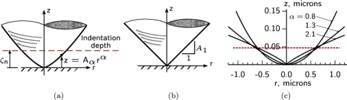
Figure 4: Contours of contact asperities as power-law surfaces of revolution: (a) general power-law form with exponent $\alpha$ and parameter $A_{\alpha}$, (b) conical asperity, and (c) asperity used in the DEM simulations (labeled $\alpha=1.3$).

For smooth spherical surfaces that conform with a particle’s radius $R$, the exponent $\alpha$ is 2 and the contour parameter $A_{2}$ is $1/(2R)$, so that Eq. (1) yields the standard Hertz solution

$$C_{2}=\frac{8}{3}\frac{G_{\text{s}}}{1-\nu_{\text{s}}}R^{1/2},\quad f^{\text{n}}=\frac{8}{3}\frac{G_{\text{s}}}{1-\nu_{\text{s}}}R^{1/2}\zeta^{3/2}$$ (2)

With a conical asperity ($\alpha$=1, Fig. 4b), $A_{1}$ corresponds to the outer slope of the cone, and

$$C_{1}=\frac{4G_{\text{s}}}{\pi(1-\nu_{\text{s}})}\frac{1}{A_{1}},\quad f^{\text{n}}=\frac{4G_{\text{s}}}{\pi(1-\nu_{\text{s}})}\frac{1}{A_{1}}\zeta^{2}$$ (3)

By decoupling the asperity shape from the more general contour of a particle’s surface, Eqs. (1) and (3) afford a free parameter $A_{\alpha}$ that can be chosen so that the DEM assembly has a $G_{\text{max}}$ similar to that of a targeted sand.

To produce simulations in which exponent $\beta=0.50$ and $G_{\text{max}}\propto p^{0.50}$, we used an asperity contour with parameter $\alpha=1.3$ (Eq. 1), forming a rounded cone whose surface lies between spherical and conical contours (Table 1 row 7 and Fig. 4c). The value 1.3 was chosen through trial and error, with the corresponding parameter $A_{1.3}$ chosen so that $G_{\text{max}}$ is close to the target value of 90MPa at a mean effective stress of 80kPa. The simulations in the paper employ this pair of values, $\alpha$ and $A_{\alpha}$. For particles of sub-mm size, such as in Nevada Sand, Eq. (1) these conditions imply an indentation depth of the asperities of a few tens of nano-meters (about 0.05 microns for $p=80$kPa) and a width of about one micron (Fig. 4c). Alternative pairs of values $\alpha$ and $A_{\alpha}$, with shapes that are more rounded and more pointed (Table 1, rows 8 and 9, and Fig. 4c) yield the exponents $\beta=0.40$ and 0.60 respectively, encompassing the range of small-strain behaviors that have been measured with sands (e.g. Table 1 footnote “f”).

A DEM simulation must also compute the tangential forces between particles, accounting both for elastic effects and for the frictional limit of force. Although tangential contact motion is often idealized as advancing steadily across a particle’s surface, DEM simulations reveal that tangential motions are quite irregular and errant and that the normal force will irregularly increase and decrease during the concurrent tangential motion [Kuhn (2011)]. The calculation of tangential force between DEM particles must account for the complex elastic-frictional response during such irregular motions, particularly when an assembly is undergoing realistic seismic loading. The tangential contact forces were calculated with an extension of Hertz-Mindlin-Deresiewicz theory [Mindlin and Deresiewicz (1953)] by using the more general Jäger contact algorithm [Jäger (2005), Kuhn (2011)]. This algorithm fully accounts for arbitrary sequences of normal and tangential contact movements in a three-dimensional setting, while maintaining the objectivity of the resulting contact forces. (The pseudo-code in Kuhn:2011a requires the modification of only two lines, 13 and 42, to accommodate the general Eq. 1.)

3 Monotonic Loading

Before conducting cyclic tests, the DEM model was calibrated and verified by comparing its monotonic undrained loading behavior with that of Nevada Sand. These tests were used to select the inter-particle friction coefficient, $\mu=0.60$. Figure 5 shows stress paths of undrained triaxial compression and extension simulations with assemblies having void ratios 0.704 and 0.746 as well as a laboratory test of Nevada Sand with void ratio 0.734 (the $D_{r}=40\%$ tests of Arulmoli1992a).

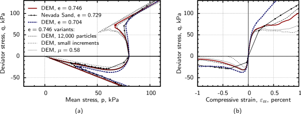
Figure 5: Undrained triaxial compression and extension of DEM simulations and Nevada Sand tests (tests CIUC40-04 and CIUE40-12 are shown, Arulmoli et al. 1992).

Heavier lines in Fig. 5 are for simulations conducted under the conditions described above and presented throughout most of the paper. Thinner lines are for variations of these conditions discussed in the next paragraph. In typical undrained laboratory tests, the pore fluid is entrapped within a saturated soil sample, preventing volume change during loading. The DEM model contains no interstitial fluid; instead, undrained, zero volume-change conditions are created by prescribing normal strains in the three coordinate directions: $(1+\varepsilon_{xx})(1+\varepsilon_{yy})(1+\varepsilon_{zz})=1$ (Fig. 1). The DEM assembly was consolidated from the initial mean effective stress of 10kPa to a mean stress $p_{\text{o}}=80$kPa, and the subsequently induced “pore water pressure” was computed from measured reductions in the mean effective stress: $\Delta u=p_{\text{o}}-p$, where $p$ is directly computed from the interparticle forces.

Loading was applied in the $z$-direction in a slow, quasi-static manner, with movements of the periodic boundaries much slower than the material’s wave speed. As in many DEM simulations, time was used as a surrogate parameter that advances deformation from one integration step to another, with sufficient steps to allow particles to adjust to the advancing deformation, thus economizing the computational run-time. A particle density much smaller than that of sand minerals was used in the simulations, a common approach in DEM analysis, which reduces the number of time steps while maintaining nearly quasi-static conditions (e.g. Thornton:1998a,OSullivan:2004c). Strain increments $\Delta\varepsilon_{zz}=\pm 5\times 10^{-7}$ in triaxial compression and extension were sufficiently small to maintain an average force imbalance per particle of less than $4\times 10^{-3}$ times the average contact force and an average assembly kinetic energy less than $5\times 10^{-4}$ of the internal elastic energy. Although nearly quasi-static, the simulations were not rate-independent. Reducing the increment $\Delta\varepsilon_{zz}$ in half softened the behavior (Fig. 5, “small increments” lines). The effect is similar to reducing the friction coefficient $\mu$ to 0.58 (also in Fig. 5). Consistent conditions of strain increment and friction coefficient were used throughout all of the simulations described below. A larger assembly of 12,000 particles was also tested (Fig. 5), but the results are nearly the same as those of the smaller assembly, which is sufficient for modeling undrained behavior.

The two DEM simulations in Fig. 5 (heavy lines) are for specimens that straddle the density of the Nevada Sand specimen, and these simulations capture the primary features found in the laboratory tests: strongly strain-softening behavior during triaxial extension that is arrested by phase-transformation at a stress $p\approx 25$kPa. At larger strains (Fig. 5a), the stress paths of the simulations converge to roughly the same critical-state slopes — in both extension and compression — as those of Nevada Sand. Because of these similarities, the same DEM parameters were applied in the remaining simulations.

The undrained behavior in simple shear is illustrated in Fig. 6 for four DEM assemblies of different densities.

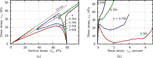
Figure 6: Undrained monotonic simple shear simulations, showing instability points ($\odot$), phase-transformation points ($\boxdot$), phase-transformation (PT) line, and critical-state (CS) line.

These undrained tests started from an isotropic stress state, and the shear strains were advanced monotonically with $\dot{\gamma}_{xz}>0$ and $\varepsilon_{xx}=\varepsilon_{yy}=\varepsilon_{zz}=\gamma_{xy}=\gamma_{yz}=0$ (see Fig. 1), as might be applied in hollow-torsion constant-height undrained laboratory tests. Unlike the triaxial conditions of Fig. 5, the directions of the principal stresses rotated during the shear loading. Markers locate the instability points ($\odot$) at which shear stress $\tau_{xz}$ reached a temporary peak and the phase-transformation points ($\boxdot$) at which the vertical effective stress $\sigma^{\prime}_{zz}$ was minimum, a state commonly ascribed to a transition from compressive to dilatant behavior. The two loosest assemblies have stress paths that display temporary instability, as would be expected with loose dry-pluviated clean sands, and these looser assemblies have more contractive behavior and lower instability and phase-transformation points than those of the denser assemblies. An interpreted phase-transformation line (PT-line) is shown in Fig. 6a, although the stress ratios $\tau_{xz}/\sigma^{\prime}_{zz}$ of the four PT points decrease slightly with increasing assembly density.

In a complementary series of drained simple-shear constant-$\sigma_{zz}$ simulations on the same assemblies, we observed transformations from compressive to dilatant behaviors for the three loosest assemblies — a transition called the characteristic-state (ChS) [Ibsen (1999)]. Our results show that the same stress ratios $\tau_{xz}/\sigma^{\prime}_{zz}$ apply to both PT and ChS transitions for the three assemblies, although the characteristic-state occurs at larger shear strains. The same drained simple-shear constant-$\sigma_{zz}$ simulations were also used to evaluate the critical-state, a condition that is attained at large strains and at which shearing progresses at constant density and shear stress. The critical-state was reached at shear strains $\gamma_{xz}$ greater than 80%, and the corresponding ratio $\tau_{xz}/\sigma^{\prime}_{zz}$ is shown as the CS-line in Fig. 6a. The critical-state void ratio is 0.912, much larger (looser) than the initial densities of the four assemblies, a result that is consistent with the PT transition to dilatant behavior observed in the undrained simulations.

4 Cyclic Simple Shear

Three types of cyclic loading sequences were simulated: (1) uniform amplitude cyclic shearing, (2) alternating and modulated sequences of small and large cyclic amplitudes, and (3) realistic, erratic sequences of seismic shearing. In all cases, cyclic shearing was uni-directional and conducted as undrained simple-shear in the horizontal $x$-direction (i.e., with shearing strains $|\gamma_{xz}|>0$ and $\gamma_{yz}=\gamma_{xy}=0$, Fig. 1). As with monotonic loading simulations, the assemblies were consolidated to an isotropic stress of 80kPa, and undrained conditions were imposed by preventing normal strains in the three coordinate directions: $\varepsilon_{xx}=\varepsilon_{yy}=\varepsilon_{zz}=0$. No ambient shear stress was imposed, corresponding to level-ground conditions. Pore water pressure was computed from the measured reductions in mean effective stress: $\Delta u=p_{\text{o}}-p$. The paper focuses primarily on four assemblies having a range of void ratios $e=0.638$ to 0.763, corresponding to relative densities $D_{r}$ in a range of about 70% to 35%.

4.1 Uniform amplitude cyclic shearing

Undrained cyclic simple shear loading was applied in a sawtooth manner: a uniform shearing rate $\pm\dot{\gamma}_{xz}$ was imposed in forward and backward directions, reversing the direction each time a target amplitude of shear stress $\tau_{xz}$ was reached (Fig. 7).

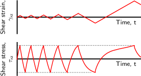
Figure 7: Loading program for uniform-amplitude cyclic simple shear.

Loading proceeded until the mean effective stress had reached zero — at initial liquefaction — and the total traversed strain $\int|d\gamma_{xz}|$ exceeded 10%. These conditions repeatedly rotated and counter-rotated the principal stress directions. The mean stress and shear stress were recorded throughout these strain-controlled histories. The four-way plot in Fig. 8 shows typical results, in this case with a cyclic stress amplitude $\tau=\pm 13$kPa (i.e., a cyclic stress ratio, CSR, $\tau_{xz}/p_{\text{o}}=0.163$).

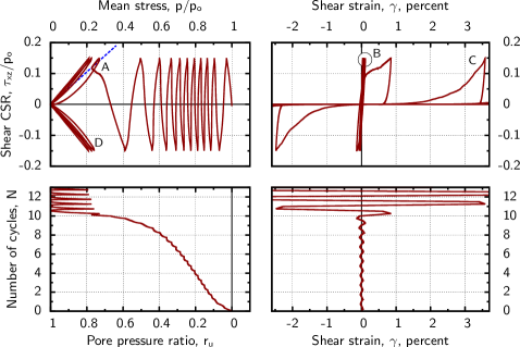
Figure 8: DEM simulation of cyclic undrained simple shear loading: $e=0.704$, $p_{\text{o}}=80$kPa, and $\tau_{xz}=13$kPa. The phase-transformation line is show in the stress path plot as a dashed line (blue in the electronic edition).

These plots show the stress path, the stress-strain evolution, and the pore pressure ratio $r_{u}=-\Delta u/p_{\text{o}}$, all of which resemble those of saturated sands. The pore pressure increases steadily, and at about 10 cycles, the stress path expresses phase-transformation behavior (labeled “A”), whereupon the mean effective stress collapses to nearly zero. Once phase-transformation has occurred, the stress-strain evolution changes from the narrow hysteresis pattern of the first 9 cycles (labeled “B”) into a broader scythe-shaped pattern (labeled “C”). Initial liquefaction ($r_{u}=1.0$) occurs after 10½ cycles of loading; and a shear strain of 3% is reached at 11 cycles. After liquefaction is initiated, the stress path falls into butterfly repetitions, typical of sands (labeled “D”). These results are qualitatively consistent with undrained cyclic shear tests of sands [Arulmoli et al. (1992), Kammerer et al. (2000), Porcino and Caridi (2007)].

Figure 9 shows the liquefaction curves obtained from multiple simulations of four assemblies having different void ratios. The upward curvature in this semi-log plot is similar to that of sands, although the curves have a steeper downward slope than with most sands (e.g. Porcino:2007a). Confirming the choice of a rounded cone asperity profile (Table 1, Row 7), simulations with a standard Hertz-Mindlin spherical contact (Table 1, Row 3) yielded an even steeper downward slope: 20–50% more cycles at large shear stress ratios and 20–30% fewer cycles at small ratios. We also obtained results for a large assembly of 12,000 particles, and the results are nearly indistinguishable from those in Fig. 9.

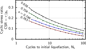
Figure 9: Liquefaction curves of four DEM assemblies.

4.2 Non-uniform cyclic sequences

Wang:1989a conducted experiments on Monterey #1 Sand in which the amplitudes of cyclic pulses were either increased or reduced during undrained loading. They found that the final pore pressure depends on the sequencing of the variable-amplitude cyclic pulses. We investigated this phenomenon with two types of simulations. With the first type, two sequences of twenty-five pulses were applied: five large-amplitude pulses were either preceded or followed by twenty small-amplitude pulses having half the amplitude of the larger pulses (Fig. 10).

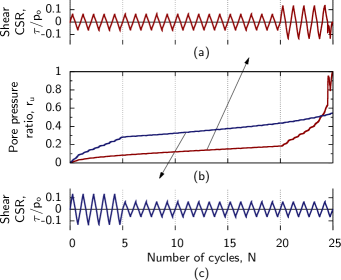
Figure 10: Simulations of two sequences of large and small cyclic pulses ($e=0.746$, $p_{\text{o}}=80$kPa).

For sequences with magnitudes large enough to produce significant pore pressures, we found that the more damaging sequences start with the smaller pulses. Figure 10 shows typical results for a loose assembly with void ratio $e=0.746$. Through trial and error, we varied the reference amplitude (i.e., that of the larger pulses), so that the full set of twenty-five pulses — twenty small followed by five large — would produce initial liquefaction ($r_{u}=1$), maintaining the ratio 1:2 of pulse amplitudes (values $\tau/p_{\text{o}}=0.067$ and 0.134 in the figure). Once the proper reference amplitude was established, we ran the alternative sequence, with the larger pulses applied first. This second sequence results in an $r_{u}$ of only 0.546. These observations are consistent with trends described by Wang:1989a. We note, however, that the difference in the effects of the two sequences is reduced with denser assemblies, and a difference is almost non-existent with the densest assembly ($e=0.638$).

In a second type of simulation, we applied a modulated sequence of rising and falling stress amplitudes (Fig. 11).

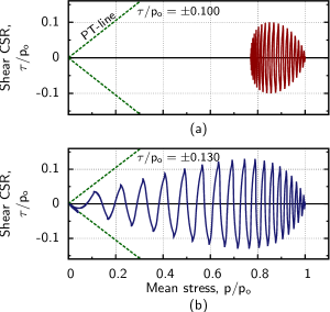
Figure 11: Simulations with modulated sequences of cyclic pulses ($e=0.746$, $p_{\text{o}}=80$kPa).

As with all other simulations, these were strain-controlled tests in the manner of Fig. 7, in which shear strain was advanced at a constant rate $\pm\dot{\gamma}_{xz}$ until a target shear stress was reached, whereupon the strain direction was reversed. The target stress of the $i$th pulse was $\tau_{i}=\tau_{\text{max}}\sin(\pi i/N)$ for the $N=20$ modulated pulses, with 10 leading (rising) pulses followed by 10 trailing (falling) pulses. When the maximum stress $\tau_{\text{max}}$ is relatively small — producing a final $r_{u}$ less than 0.5 — the leading pulses are more damaging than the trailing pulses. This result is apparent in the stress path at the top of Fig. 11, where the stress path is more elongated to the right. With a larger $\tau_{\text{max}}$, the opposite trend is observed: the trailing pulses produce a larger rise in pore pressure, resulting in a stress path that is elongated toward the left (bottom of Fig. 11).

4.3 Seismic loading

In a final series of simulations, we applied 24 transient seismic loading sequences to four assemblies of 6400 particles having different void ratios. By analyzing the simulation results, we propose a Severity Measure (SM) that predicts the onset of liquefaction, based on shear stress records. A suite of 24 ground motions was selected from the NGA database maintained by the Pacific Earthquake Engineering Research (PEER) Center [PEER (2000)]. The selected ground motions were screened from about 4000 candidate motions to provide a diversity of spectral and temporal conditions as determined with four intensity measures (IMs): PGA/MSF (peak ground acceleration with a magnitude scaling factor, e.g. Arango:1996a); Arias intensity [Kayen and Mitchell (1999)]; CAV₅ intensity (cumulative absolute velocity, Kramer:2006a); and NED intensity (normalized energy demand, Green:2001a). Each of the 24 motions produced a large value of one IM but a low value of another IM, all in various combinations of IM pairs, thus providing a suite of 24 motions with significantly different amplitudes, frequency contents, durations, and phasing relationships.

These ground acceleration records can not be input directly into the DEM model. Shear stress histories were extracted from the ground accelerations by applying these motions as inputs in an equivalent-linear wave propagation model of a 6m sand layer using the ProShake software. The resulting stress histories were in the form of cyclic shear stress ratio records (CSR records) of shearing stress divided by the initial vertical confining stress, $\tau_{xz}/\sigma_{zz,\text{o}}$ ($\tau_{xz}/p_{\text{o}}$ in our isotropically consolidated simulations). Rather than applying a CSR record directly, the record was processed in two ways. First, the CSR record was digitally perused to identify all of its reversals of loading direction. These peaks and valleys became the target shearing stresses at which the direction of the shearing strain $\pm\dot{\gamma}_{xz}$ was reversed while shearing with the same rate magnitude (see Fig. 7).

A second modification was applied at the start of a simulation: the stresses of each CSR record were scaled by a factor $\Phi$ so that initial liquefaction was delayed until the very end of the record. A different scaling factor $\Phi$ was required for each of the 24 CSR records, and the factors would also differ among the four assemblies having different void ratios. The necessary factors were determined through a trial and error procedure for each of the 24 records and for each void ratio. Figure 12 shows the results of a single scaled CSR record for a DEM assembly with void ratio $e=0.704$. The scaled record of CSR versus time is shown in the lower left of the plot. The factor $\Phi=0.647$ in this figure causes the assembly to reach an $r_{u}=0.932$ at the end of the record. Increasing $\Phi$ to 0.648 pushes the assembly beyond initial liquefaction, producing a few small “butterfly” oscillations at the end of the stress path (as in Fig. 8).

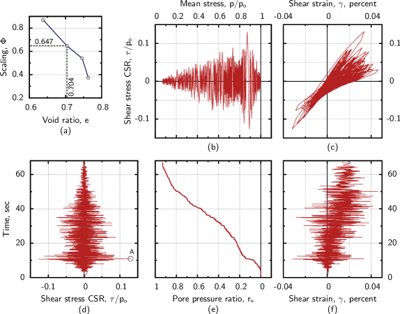
Figure 12: Seismic loading of a DEM assembly, $e=0.704$, $p_{\text{o}}=80$kPa. The record of cyclic stress ratios ($\text{CSR}=\tau_{xz}/p_{\text{o}}$) is from the PEER NGA record LANDERS/MCF000. Shear stresses are scaled by factor $\Phi=0.647$ to suspend initial liquefaction until the end of the CSR record. The upper-left insert shows the dependence of $\Phi$ on the assembly void ratio $e$.

Although arriving at the proper factors $\Phi$ is a time-consuming process, this process serves three purposes:

1. The factor $\Phi$ provides a quantifiable basis for ranking the severities of the 24 original (unscaled) CSR records with respect to their propensity for producing initial liquefaction ($r_{u}=1$). Specifically, the inverse of each factor, $1/\Phi$, is a measure of the severity of the particular ground motion and its shearing record (i.e., the original unscaled CSR record). The 24 records are ranked in Fig. 13, with the most severe records at the top and the most benign at the bottom. The ranking in this figure was derived from the single assembly with void ratio $e=704$. The scaled CSR record of Fig. 12 appears near the middle of the ranking (labeled $\odot$ in Fig. 13).

   

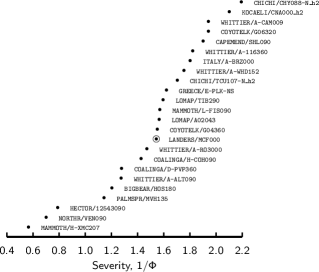
   Figure 13: Ranking of severities $1/\Phi$ of 24 seismic CSR records ($e=0.704$, $p_{\text{o}}=80$kPa). Records near the top are the most severe, requiring a small $\Phi$ to forestall liquefaction until the end of the record.

2. Having scaled all 24 shear stress records so that each postponed initial liquefaction until the end of the record, we can seek a commonality in their (scaled) features. That is, we can explore possible severity measures (SMs), which we define as a scalar value, derived from a cyclic stress history (CSR record), that measures the record’s propensity for producing initial liquefaction. For example, the peak shear stress in a CSR record (e.g., the single point “A” in the lower left of Fig. 12) could serve as a simple (albeit inefficient) severity measure. An ideal SM would have the same scalar value for each of the 24 scaled CSR records, since each record is scaled to reach a common state of initial liquefaction at the end of the record. The range of the 24 SM values for the scaled records is an indicator of the efficiency of a candidate SM. Although many candidate SMs were investigated, the paper gives results for four SMs, described below.

3. Besides its use as a predictor of initial liquefaction, an ideal severity measure would also predict other damaging effects of a particular seismic record. These effects could include pore pressure rise ($\Delta u$ or $r_{u}$) for CSR records that are not sufficiently severe to initiate liquefaction, post-liquefaction strains for more severe records, etc.

We address the first and second items and also apply a particular Severity Measure (SM) to the prediction of pore pressure rise, as suggested in the third item.

The key to this approach is finding the scaling factor $\Phi$ of each seismic CSR record that would postpone the onset of liquefaction until the very end of the record. For this purpose, we made use of a primary advantage of DEM simulations: the ability to repeatedly subject the same assembly (i.e. virtual specimen) to the 24 records, each with different scaling factors $\Phi$, thus finding the proper factors by trial and error. Ten or eleven trials were usually necessary with each CSR record to find its $\Phi$ with a precision of $\pm 0.001$. This same procedure was applied to all four assemblies having different void ratios.

The severities of the 24 records are shown in the slope-graph of Fig. 14 for the four assemblies.

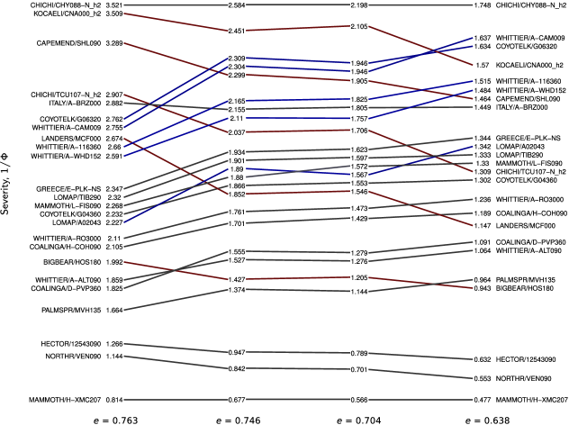
Figure 14: Slope-graph showing the rankings of severities $1/\Phi$ of 24 seismic CSR records, based upon simulations with four densities.

In this figure, the records are ranked from the most severe (top, large $1/\Phi$) to the least severe (bottom), with density increasing from left to right (the ranking in Fig. 13 is reproduced as the third column in Fig. 14). Because denser assemblies are more resistant to initial liquefaction, the scaling factor $\Phi$ of each CSR record must be increased with each increase in density (for example, with the CHICHI/CHY088-N_h2 record at the top of Fig. 14, the inverse factor $1/\Phi$ is reduced from 3.521 to 1.748 as the void ratio decreases from 0.763 to 0.638). The ranking of the 24 records is not consistent across the four densities, as is apparent from the crossing lines. Oddly, the severities of certain CSR records, relative to other records, decrease with increasing density (these records are marked red in the electronic version); whereas, the severities of other records increase relative to other records at greater density (marked blue). For example, the LANDERS/MCF000 record is much more severe than the LOMAP/A02043 record when applied to the loosest assembly; but these roles are reversed with the densest assembly. This anomalous density-dependent behavior was also noted in a previous section regarding non-uniform sequences of large and small shearing pulses.

Many scalar severity measures (SMs) were explored as candidates for predicting the propensity of a particular cyclic stress ratio (CSR) record for producing initial liquefaction. Four representative SMs are as follows:

$$\text{SM}_{1}= \left|\tau_{\text{max}}/p_{\text{o}}\right|$$ (4)

$$\text{SM}_{2}= \int\frac{\tau\,d\gamma^{\text{plastic}}}{p_{\text{o}}}$$ (5)

$$\text{SM}_{3}= \int H(|\gamma|-\gamma_{\text{t}})\,\left|d\gamma\right|$$ (6)

$$\text{SM}_{4}= \int\left|d\left[\left(\frac{|\tau|}{p}\right)^{2}\right]\right|=2\int\frac{|\tau|}{p}\,\left|\frac{d|\tau|}{p}-\frac{|\tau|}{p}\frac{dp}{p}\right|$$ (7)

which represent the maximum shear ratio of a CSR record (SM₁), a normalized energy demand (SM₂), a strain-path measure (SM₃), and a stress-path measure (SM₄). For the uni-directional loading of our DEM simulations, $\tau$ is the shear stress $\tau_{xz}$; $\gamma$ is the shear strain $\gamma_{xz}$; $\gamma_{\text{t}}$ is a threshold shear stress (assumed to be 0.01%); $H()$ is the Heaviside function, which equals zero unless the current strain magnitude $|\gamma_{xz}|$ exceeds $\gamma_{\text{t}}$ (in which case, $H=1)$; $p_{\text{o}}$ is the initial mean effective stress; and $p$ is the current mean effective stress. The plastic strain increment $d\gamma^{\text{plastic}}$ in Eq. (5) is computed by subtracting the elastic increment $d\tau/G_{\text{max}}$ from the full strain increment $d\gamma$, where modulus $G_{\text{max}}$ is estimated with the relation given in Table 1, row 7. Unlike earthquake intensity measures such as the Arias intensity, these four SMs are not based upon ground motions (accelerations or velocities) but instead are integrals of the stresses and strains that result from these ground motions. We also note that the four SMs are rate-independent, as time is not explicitly part of their definitions. The liquefaction resistance of sands is known to be insensitive to the loading rate (i.e. nearly independent of excitation frequency), which is consistent with the four SMs. If a time history of shear stress or strain is available, the differential quantities in Eqs. (5)–(7) can be replaced with the corresponding rate differentials: for example $d\tau=(d\tau/dt)\,dt$.

These four SMs were evaluated for the 24 seismic stress (CSR) records. Each simulation yields a record of shear strain $\gamma_{xz}$ and mean effective stress $p$ as well as the input stresses $\tau_{xz}$, permitting evaluation of integrals (5)–(7). As stated before, a scaling factor $\Phi$ was determined for each CSR record that would delay initial liquefaction until the end of the record, and the resulting 24 scaled SM values correspond to a common state of initial liquefaction ($r_{u}=1$), as will be denoted with a subscript “$\Phi$”. Figure 15 shows box plots of the four SMs in which their values from the 24 scaled CSRs ($\text{SM}_{i\Phi}$, $i=1,2,3,4$) are normalized by dividing by the mean of the particular SM, denoted as $\left\langle\text{SM}_{i\Phi}\right\rangle$.

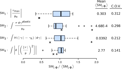
Figure 15: Efficiencies of four severity measures (SMs): box plots of 24 cyclic stress records, scaled to produce initial liquefaction ($e=0.746$, $p_{\text{o}}=80$kPa). Values for the non-uniform sequence of Fig. 10 (top) are marked “$+$”; values for the sequence of Fig. 11 (bottom) are marked “$\times$”.

The scatter in the simplest measure, $\text{SM}_{1\Phi}$, is considerable, indicating that maximum shear stress is a poor predictor of liquefaction. Although $\text{SM}_{2\Phi}$, $\text{SM}_{3\Phi}$, and $\text{SM}_{4\Phi}$ exhibit smaller dispersions, the stress-path measure $\text{SM}_{4}$ has the least scatter, indicating a superior efficiency in predicting initial liquefaction. The efficiencies of the four SMs are summarized in the inset of Fig. 15, giving their coefficients of variation (standard deviation divided by mean), with smaller coefficients corresponding to a more efficient and less scattered severity measure. The measure $\text{SM}_{4}$ of Eq. (7) yields the lowest dispersion and serves as an efficient predictor of initial liquefaction.

Figure 15 also shows results of applying the four severity measures to the non-uniform cyclic sequences illustrated in Figs. 10 and 11. Two of these sequences resulted in liquefaction (Fig. 10 top and Fig. 11 bottom). Although three of the severity measures were poor predictors of liquefaction (the “$+$” and “$\times$” symbols in Fig. 10), the fourth measure $\text{SM}_{4}$ gave values close to the threshold liquefaction value $\left\langle\text{SM}_{4\,\Phi}\right\rangle$. In contrast, the two-amplitude sequence at the bottom of Fig. 10 did not result in liquefaction, a result that is consistent with its low SM value: $\text{SM}_{4}/\left\langle\text{SM}_{4\,\Phi}\right\rangle=0.54$.

The value of an SM required to initiate liquefaction will depend upon a soil’s density. Figure 16 gives the values of SM_4Φ for four specimens having different void ratios, based upon the averaged results of the 24 seismic sequences.

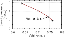
Figure 16: Effect of specimen density on the average value of severity measure $\langle\text{SM}_{4\Phi}\rangle$ (Eq. 7) at initial liquefaction.

As would be expected, the value of SM₄ required to initiate liquefaction (i.e., SM_4Φ) increases with increasing specimen density.

A proper measure of the severity of a cyclic sequence should also predict the pre-liquefaction rise in pore pressure. Figure 17 shows the relationship between the excess pore pressure ratio $r_{u}=1-p/p_{\text{o}}$ and SM₄ for a single assembly subjected to the 24 seismic records.

Figure 17: Relationship between severity measure SM_4Φ (Eq. 7) and excess pore pressure ratio $r_{u}$ ($e=0.746$, $p_{\text{o}}=80$kPa).

This severity measure is a monotonically increasing function of the shear stress history (scaled CSR record), which is seen to advance in a roughly linear manner with increasing pore pressure. Figure 17 shows only modest scatter in the SM₄ vs. $r_{u}$ behavior, indicating that this severity measure would serve as an efficient predictor of pore pressure rise.

5 Concluding Remarks

A discrete element (DEM) assembly of virtual particles has been calibrated to approximate the behavior of a natural sand, particularly at small strains. The paper presents simulation methodologies for exploring the complex response of such granular materials to undrained cyclic loading. Methods are also proposed for using simulations to rank the severities of different seismic sequences and for developing scalar predictors of the severity. Some anomalous behaviors have been observed, and a promising scalar predictor of liquefaction susceptibility is identified. Even though laboratory tests are the final arbiter of a material’s behavior, DEM simulations offer certain capabilities that are difficult to achieve in a laboratory setting: in particular, the ability to subject the same virtual assembly to nearly unlimited loading sequences.

Natural extensions of the current work would include simulations of bi-directional seismic shearing and of seismic loading in sloping-ground conditions. Even with its advantages, DEM simulations continue to be hampered by the computational demands of effectively simulating large, realistic boundary-value problems (foundations, excavations, etc.) or even conducting small element tests well into the post-liquefaction regime in which the strain excursions become very large. We believe, however, that discrete element simulations can serve to investigate many important aspects of the complex cyclic behavior of soils.

References

- Agnolin and Roux (2007) Agnolin, I. and Roux, J.-N. (2007). “Internal states of model isotropic granular packings. iii. elastic properties.” Phys. Rev. E, 76, 061304.
- Arango (1996) Arango, I. (1996). “Magnitude scaling factors for soil liquefaction evaluations.” J. Geotech. and Geoenv. Eng., 122(11), 929–936.
- Arulanandan and Scott (1993) Arulanandan, K. and Scott, R. F. (1993). “Project VELACS—control test results.” J. Geotech. Eng., 119(8), 1276–1292.
- Arulmoli et al. (1992) Arulmoli, K., Muraleetharan, K. K., Hossain, M. M., and Fruth, L. S. (1992). “VELACS verification of liquefaction analyses by centrifuge studies laboratory testing program soil data report.” Report No. Project No. 90-0562, The Earth Technology Corporation, Irvine, CA. Data available through http://yees.usc.edu/velacs.
- Ashmawy et al. (2003) Ashmawy, A. K., Sukumaran, B., and Hoang, V. V. (2003). “Evaluating the influence of particle shape on liquefaction behavior using discrete element modeling.” Proc. of the 13th Intl. Offshore and Polar Engrg. Conf., Vol. 2, ISOPE, Honolulu, 542–549.
- Cavarretta et al. (2010) Cavarretta, I., Coop, M., and O’Sullivan, C. (2010). “The influence of particle characteristics on the behaviour of coarse grained soils.” Géotechnique, 60(6), 413–423.
- Cho et al. (2006) Cho, G.-C., Dodds, J., and Santamarina, J. C. (2006). “Particle shape effects on packing density, stiffness, and strength: natural and crushed sands.” J. Geotech. and Geoenv. Eng., 132(5), 591–602.
- Cole et al. (2010) Cole, D. M., Mathisen, L. U., Hopkins, M. A., and Knapp, B. R. (2010). “Normal and sliding contact experiments on gneiss.” Granul. Matter, 12, 69–86.
- Dobry and Ng (1992) Dobry, R. and Ng, T.-T. (1992). “Discrete modelling of stress-strain behaviour of granular media at small and large strains.” Eng. Comput., 9, 129–143.
- Duku et al. (2008) Duku, P. M., Stewart, J. P., Whang, D. H., and Yee, E. (2008). “Volumetric strains of clean sands subject to cyclic loads.” J. Geotech. and Geoenv. Eng., 134(8), 1073–1085.
- El Shamy and Zamani (2012) El Shamy, U. and Zamani, N. (2012). “Discrete element method simulations of the seismic response of shallow foundations including soil-foundation-structure interaction.” Int. J. Numer. and Anal. Methods in Geomech., 36(10), 1303–1329.
- El Shamy and Zeghal (2005) El Shamy, U. and Zeghal, M. (2005). “Coupled continuum-discrete model for saturated granular soils.” J. Eng. Mech., 131(4), 413–426.
- Goddard (1990) Goddard, J. D. (1990). “Nonlinear elasticity and pressure-dependent wave speeds in granular media.” Proc. R. Soc. Lond. A, 430, 105–131.
- Green (2001) Green, R. A. (2001). “Energy-based evaluation and remediation of liquefiable soils.” Ph.d. dissertation, Virginia Polytechnic Institute and State Univ., Blacksburgh, VA.
- Hakuno and Tarumi (1988) Hakuno, M. and Tarumi, Y. (1988). “A granular assembly simulation for the seismic liquefaction of sand.” Proc. Jap. Soc. Civil Eng., 398(10), 129–138.
- Hardin (1978) Hardin, B. O. (1978). “The nature of stress-strain behavior of soils.” Earthquake Engineering and Soil Dynamics–Proceedings of the ASCE Geotechnical Engineering Division Specialty Conference, June 19-21, 1978, Pasadena, CA, Vol. 1, Pasadena, CA, ASCE, 3–90.
- Ibsen (1999) Ibsen, L. B. (1999). “The mechanism controlling static liquefaction and cyclic strength of sand.” Physics and Mechanics of Soil Liquefaction, P. V. Lade and J. A. Yamamuro, eds., Balkema, Rotterdam, 29–39.
- Jäger (1999) Jäger, J. (1999). “Uniaxial deformation of a random packing of particles.” Arch. Appl. Mech., 69(3), 181–203.
- Jäger (2005) Jäger, J. (2005). New Solutions in Contact Mechanics. WIT Press, Southampton, UK.
- Kammerer et al. (2000) Kammerer, A. M., Wu, J., Pestana, J. M., Riemer, M., and Seed, R. B. (2000). “Cyclic simple shear testing of Nevada Sand for PEER Center project 2051999.” Geotechnical Engineering Report UCB/GT/00-01, Univ. of California, Berkeley, Dept. of Civil and Environmental Engineering.
- Kayen and Mitchell (1999) Kayen, R. E. and Mitchell, J. K. (1999). “Assessment of liquefaction potential during earthquakes by Arias intensity.” J. Geotech. and Geoenv. Eng., 123(12), 1162–1174.
- Kramer and Mitchell (2006) Kramer, S. L. and Mitchell, R. A. (2006). “Ground motion intensity measures for liquefaction hazard evaluation.” Earthq. Spectra, 22(2), 413–438.
- Kuhn (2002) Kuhn, M. R. (2002). “OVAL and OVALPLOT: programs for analyzing dense particle assemblies with the Discrete Element Method.” http://faculty.up.edu/kuhn/oval/oval.html.
- Kuhn (2011) Kuhn, M. R. (2011). “Implementation of the Jäger contact model for discrete element simulations.” Int. J. Numer. Methods Eng., 88(1), 66–82.
- Mindlin and Deresiewicz (1953) Mindlin, R. and Deresiewicz, H. (1953). “Elastic spheres in contact under varying oblique forces.” J. Appl. Mech., ASME, 19(1), 327–344.
- Mitchell and Soga (2005) Mitchell, J. K. and Soga, K. (2005). Fundamentals of soil behavior. John Wiley & Sons, 3rd edition.
- Ng and Dobry (1994) Ng, T.-T. and Dobry, R. (1994). “Numerical simulations of monotonic and cyclic loading of granular soil.” J. Geotech. Eng., 120(2), 388–403.
- O’Sullivan et al. (2004) O’Sullivan, C., Cui, L., and Bray, J. D. (2004). “Three-dimensional discrete element simulations of direct shear tests.” Numerical Modeling in Micromechanics Via Particle Methods: Proceedings of the Second International PFC Symposium, Y. Shimizu, R. Hart, and P. Cundall, eds., Taylor & Francis, London, UK, 373–382.
- PEER (2000) PEER (2000). “Pacific earthquake engineering research center PEER strong motion database.” Pacific Earthquake Engineering Research Center, http://peer.berkeley.edu/smcat/.
- Pestana and Whittle (1995) Pestana, J. M. and Whittle, A. J. (1995). “Compression model for cohesionless soils.” Géotechnique, 45(4), 611–631.
- Porcino and Caridi (2007) Porcino, D. and Caridi, G. (2007). “Pre-and post-liquefaction response of sand in cyclic simple shear.” GEO-Denver 2007: New Peaks in Geotechnics, Dynamic Response and Soil Properties (GSP 160) Denver.
- Salot et al. (2009) Salot, C., Gotteland, P., and Villard, P. (2009). “Influence of relative density on granular materials behavior: DEM simulations of triaxial tests.” Granul. Matter, 11(4), 221–236.
- Santamarina and Cascante (1998) Santamarina, C. and Cascante, G. (1998). “Effect of surface roughness on wave propagation parameters.” Géotechnique, 48(1), 129–136.
- Sazzad and Suzuki (2010) Sazzad, M. and Suzuki, K. (2010). “Micromechanical behavior of granular materials with inherent anisotropy under cyclic loading using 2d dem.” Granul. Matter, 12(6), 597–605.
- Simmons and Brace (1965) Simmons, G. and Brace, W. F. (1965). “Comparison of static and dynamic measurements of compressibility of rocks.” J. Geophys. Res., 70(22), 5649–5656.
- Sitharam (2003) Sitharam, T. G. (2003). “Discrete element modelling of cyclic behaviour of granular materials.” Geotech. & Geol. Eng., 21, 297–329.
- Thornton and Antony (1998) Thornton, C. and Antony, S. J. (1998). “Quasi-static deformation of particulate media.” Phil. Trans. Roy. Soc. Lond. A, 356(1747), 2763–2782.
- Walton (1987) Walton, K. (1987). “The effective elastic moduli of a random packing of spheres.” J. Mech. Phys. Solids, 35(2), 213–226.
- Wang and Kavazanjian (1989) Wang, J. N. and Kavazanjian, E. (1989). “Pore pressure development during non-uniform cyclic loading.” Soils and Found., 29(2), 1–14.
- Wichtmann and Triantafyllidis (2009) Wichtmann, T. and Triantafyllidis, T. (2009). “Influence of the grain-size distribution curve of quartz sand on the small strain shear modulus.” J. Geotech. and Geoenv. Eng., 135(10), 1404–1418.
- Zettler et al. (2000) Zettler, T. E., Frost, J. D., and DeJong, J. T. (2000). “Shear-induced changes in smooth HDPE geomembrane surface topography.” Geosynth. Intl., 7(3), 243–267.