Causal faster than light travel from travel-localized second time coordinate

Horatiu Nastase^a

^aInstituto de Física Teórica, UNESP-Universidade Estadual Paulista

R. Dr. Bento T. Ferraz 271, Bl. II, Sao Paulo 01140-070, SP, Brazil

Abstract

I present a general relativistic model with a compactified second time coordinate that a priori allows for causal, yet faster than light travel in the background of a FLRW geometry, by local modification of a higher dimensional background geometry, specifically with respect to the radius of the compactified time coordinate. The modification can be induced via the fields of the model. I show that one cannot convert (as possible in special relativistic models, or simple general relativistic models) the super-luminality into closed time-like loops violating causality, due to a novel combination of factors, at least for $v_{\rm max}\leq\sqrt{2}$. The physics of the second time is constrained by postulates derived from reasonable physical assumptions. I comment on the possibility of experimental implications of the model.

1 Introduction

Since Einstein wrote his special relativistic and general relativistic theories, people have been wondering whether it is possible in principle to travel faster than the speed of light. In special relativity, the answer is a definite NO: first, the energy and momentum required to reach the speed of light increases to infinity as $v\rightarrow c$; second, there are imaginary quantities involved for $v>c$; and third, assuming the existence of a particle with $v>c$, one can construct, by boosting, a closed time-like loop that will violate causality, as I will review later on. In 3+1 dimensional general relativity, the answer is a bit more nuanced: there is one notion, first thought of in science fiction, of a local disturbance in the gravitational field, a “warp drive”, a concrete proposal for which was put forward in [1], that would a allow a spaceship to travel faster than light with respect to an ambient Minkowski space, even though locally the ship would always have $v\leq c$. There are several problems with the explicit proposal in [1], starting with the fact that there is no solution to Einstein’s equations, as the metric $g_{\mu\nu}$ is just stated; continuing with the fact that it would require “matter” (obtained as $T_{\mu\nu}$ being by definition $\frac{1}{8\pi G_{N}}(R_{\mu\nu}-\frac{1}{2}g_{\mu\nu}R)$) that violates the energy conditions; and finally dealing with the same problem, of being able, within the ambient Minkowski space, to create a closed time-like loop that violates causality (perhaps there are others objections, but here I focus on these ones). Violations of the energy conditions in general relativity can have other effects that lead to superluminal motion and violations of causality, from the example of the Morris-Thorne traversable wormhole [2] (a trip through it amounts to superluminal motion), to more recent attempts to create suitable cosmologies, where the focus is on excluding successfully such parameter space from the theory in order to be consistent, e.g. [3]. The null energy condition can be violated in the quantum theory, and thus resulting in a minute superluminality, which however cannot be made macroscopic and/or observable (the earliest paper I know of being [4]).

An unrelated way to a priori obtain superluminality is to introduce a second time coordinate. For such a space, in the absence of any new physics criterion, the violation of causality goes hand in hand with superluminality and is easily explained: the second time can change, allowing spatial motion, while the first time is unchanged, and one can easily obtain a closed time-like loop, especially if the second time coordinate is considered to be compactified (since then the second time coordinate is a loop). One can then impose constraints such that only one time is effective, obtaining causal, but sub-luminal physics, as in the long program of two-time physics developed by Itzhak Bars and collaborators (some of the relevant references being [5, 6, 7, 8, 9]).

In this paper, however, I want to show that if one considers a few physical conditions, concretized in some principles, as well as adding some somewhat obvious field to the theory, consistent with both the principles and observations, we find a theory that has the potential to have causal superluminality. Physics still has effectively one time only, through a constraint arising from the principles, and as observed in everyday life, but the presence of the second time can lead to superluminality (from the point of a fictitious Minkowskian background that we can use for observations), provided one can find a way to excite a field of the theory. I will show that it is now impossible to construct a closed timelike loop using the superluminality. A necessary ingredient is the existence of a spontaneous breaking of the (fictitious) Lorentz invariance consistent with the presence of the background FLRW cosmology, as previewed in [10].

The paper is organized as folllows. In section 2 I describe the model with compactified time. In section 3 I introduce some physical principles, and resulting from them, I quantify the apparent Lorentz violation. In section 4, I describe the fact that this violation can be nevertheless causal. In section 5, I present some observations on fields and quantization in the presence of the second time, and some ideas about observational consequences, and in section 6 I conclude.

2 Compactified second time and model

The basic idea of the paper is that we are in a general relativistic theory, and there is a small, compactified, second time-like coordinate, so that in a certain gauge for general coordinate invariance (meaning that we can put $g_{0i}=0$), we have

$$ds^{2}=-|g_{00}|dt^{2}-|g_{0^{\prime}0^{\prime}}|dt^{\prime 2}+g_{ij}dx^{i}dx^{j}\;,$$ (2.1)

but where $t^{\prime}$ is periodic with a small period (radius). In the following, I will always denote this second time with $t^{\prime}$, or $x^{0^{\prime}}$. Additionally, I will use theorist’s units and put the speed of light in Minkowski space (at least with respect to the usual time $t$) to one, $c=1$, and denote by $x^{i}$ the 3 large spatial coordinates that we observe (there could be more compact spatial coordinates, like in string theory for instance, but we will ignore those in this paper).

I will also assume that the periodicity of $t^{\prime}$ is $2\pi R_{0}$, meaning that $t^{\prime}$ is dimensionful like $t$, and then $|g_{0^{\prime}0^{\prime}}|=R^{2}/R_{0}^{2}$ measures the radius in units of $R_{0}$. Moreover, I will assume that $|g_{0^{\prime}0^{\prime}}|=\epsilon\ll 1$. We will specify the meaning of $R_{0}$, and the splitting of the periodicity into $R_{0}$ and $\sqrt{\epsilon}$, in the next section.

The implication of the condition $|g_{0^{\prime}0^{\prime}}|\ll 1$ is that under normal circumstances, the path of light, $ds^{2}=0$, is mostly unaffected by the extra term. But if we can increase $|g_{0^{\prime}0^{\prime}}|$, thought of as a scalar field that can condense, just like in any regular Kaluza-Klein model, we can have an observable effect. The condensation of $\phi$ can be driven by some other matter field, which we must define.

If gravity is coupled to matter, the natural candidate that can interact with the metric and condense $\phi$ is an antisymmetric tensor field strength. Since the background spacetime is actually the cosmological FLRW metric for the expanding Universe, such a metric has a preferred Lorentz frame with respect to the tangent Minkowski space, valid in a small neighbourhood (since Lorentz invariance is not a symmetry of the FLRW metric). This defines the cosmic time $t$ in the metric, and an apparent “spontaneous breaking of Lorentz invariance”: to be more precise, since we are in general relativity, we only have local Lorentz invariance, which is always preserved, but global Lorentz invariance is broken by the choice of time in the FLRW metric. This is why we can detect the Earth’s motion with respect to the system of the CMBR, which defines the cosmic time. That means that in the FLRW metric, we can have a special vector with only nonzero component $A_{0}$ (where $x^{0}$ here is the cosmic time), or equivalently a special 3-index antisymmetric tensor with spatial components only, $F_{ijk}$, with a single independent component, $F_{123}$, as considered in [10].

Since we want to have an extra time direction, we can have a possible 4-index antisymmetric tensor, with only nonzero independent component $F_{(4)0^{\prime}123}$. Since this should be the field that condenses, $\phi$, we want that there is a field strength $F_{(4)MNPQ}$ interacting with gravity, where we denote by $M,N,...=0,0^{\prime},1,2,3$ the (3+2)-dimensional space, and by $\mu,\nu,...=0,1,2,3$ the (3+1)-dimensional space. We want that normally, $c=1$ should be the maximum speed, so we must have $|g_{0^{\prime}0^{\prime}}|=\epsilon\ll 1$ normally, and then $F_{(4)0^{\prime}123}\simeq 0$ as well, but when $F_{(4)MNPQ}\neq 0$, we want $|g_{0^{\prime}0^{\prime}}|\neq 0$ (i.e., macroscopic, or of order one) also.

2.1 Model and its equations of motion

The action for the model is then

$$S = \frac{M^{3}_{\rm Pl,5}}{2}\int d^{5}x\sqrt{+g^{(5)}}R^{(5)}+\frac{M^{3}}{2}\int d^{5}x\sqrt{+g^{(5)}}f\left|\frac{1}{4!}F_{(4)MNPQ}F_{(4)}^{MNPQ}-m^{2}\right|$$ (2.3)

$$+\int\sqrt{+g^{(5)}}{\cal L}_{\rm matter}.$$

Here $M_{\rm Pl,5}$ is a 5-dimensional Planck scale, $M$ is an independent quantity, $g^{(5)}>0$ since we have a 3+2 dimensional signature, ${\cal L}_{\rm matter}$ is the Lagrangian for matter other than $A_{(3)MNP}$ and of $m$, $F_{(4)MNPQ}=4\partial_{[M}A_{NPQ]}$ (total antisymmetrization with strength one), so that $F_{(4)}=dA_{(3)}$ in form language, and $m$ is a quantum VEV of matter fields, about which we will say more later on. Moreover, $f$ is a scalar function that will be defined shortly in several cases, and the absolute value in this term is present only in the $f=1$ case.

For economy of the model, we can choose $M=M_{\rm Pl,5}$, which avoids annoying factors of $M^{3}/M_{\rm Pl,5}^{3}$, which can otherwise be reabsorbed in the definitions of $A_{(3)MNP}$ and $m$.

Consider its equations of motion, under the dimensional reduction ansatz for the metric with respect to $t^{\prime}$,

$$\partial_{0^{\prime}}g_{MN}=0.$$ (2.4)

The most relevant component is the Einstein equation of $g_{0^{\prime}0^{\prime}}$.

On the ansatz, we calculate first

$$R_{0^{\prime}0^{\prime}} = \partial_{M}{\Gamma^{M}}_{0^{\prime}0^{\prime}}+{\Gamma^{M}}_{NM}{\Gamma^{N}}_{0^{\prime}0^{\prime}}-{\Gamma^{M}}_{N0^{\prime}}{\Gamma^{N}}_{M0^{\prime}}$$ (2.5)

$${\Gamma^{M}}_{0^{\prime}0^{\prime}} = -\frac{1}{2}g^{MN}\partial_{N}g_{0^{\prime}0^{\prime}}$$ (2.6)

$${\Gamma^{M}}_{0^{\prime}N} = \frac{1}{2}g^{MP}(\partial_{N}g_{P0^{\prime}}-\partial_{P}g_{N0^{\prime}})\Rightarrow$$ (2.7)

$${\Gamma^{M}}_{0^{\prime}M} = 0\;,$$ (2.8)

obtaining

$$R_{0^{\prime}0^{\prime}} = -\frac{1}{2}\partial^{M}\partial_{M}g_{0^{\prime}0^{\prime}}-\frac{1}{2}(\partial^{\mu}g_{0^{\prime}0^{\prime}}){\Gamma^{M}}_{\mu M}-\frac{1}{4}(\partial^{Q}g_{P0^{\prime}}$$ (2.10)

$$-g^{NQ}\partial_{P}g_{N0^{\prime}})(\partial^{P}g_{Q0^{\prime}}-g^{MP}\partial_{Q}g_{M0^{\prime}}).$$

Next, we use the identities

$${\Gamma^{M}}_{\mu M} = {\Gamma^{\nu}}_{\mu\nu}+\frac{1}{2}g^{0^{\prime}0^{\prime}}(\partial_{\mu}g_{0^{\prime}0^{\prime}})\Rightarrow$$ (2.11)

$$D_{\mu}^{(5)}\partial^{\mu} = \partial_{M}\partial^{M}+{\Gamma^{M}}_{\mu M}\partial^{\mu}=D_{\mu}^{(4)}\partial^{\mu}+\frac{1}{2}g^{0^{\prime}0^{\prime}}(\partial_{\mu}g_{0^{\prime}0^{\prime}})\partial^{\mu}\;,$$ (2.12)

to finally write $R_{0^{\prime}0^{\prime}}$ in the form

$$R_{0^{\prime}0^{\prime}}=-\frac{1}{2}D_{\mu}^{(4)}\partial^{\mu}g_{0^{\prime}0^{\prime}}+\frac{1}{4}g^{0^{\prime}0^{\prime}}(\partial_{\mu}g_{0^{\prime}0^{\prime}})(\partial^{\mu}g_{0^{\prime}0^{\prime}}).$$ (2.13)

The first observation then is that the Eistein equations in vacuum (for no matter contribution, and $F_{(4)MNPQ}\simeq 0\simeq m$), in particular the $0^{\prime}0^{\prime}$ component,

$$R_{0^{\prime}0^{\prime}}-\frac{1}{2}g_{0^{\prime}0^{\prime}}R=0\;,$$ (2.14)

is solved by

$$g_{0^{\prime}0^{\prime}}=\epsilon\rightarrow 0\;,$$ (2.15)

since in that case we also obtain

$$R_{0^{\prime}0^{\prime}}\rightarrow 0.$$ (2.16)

Moreover, the contribution of $g_{0^{\prime}0^{\prime}}$ to the $R_{\mu\nu}$ components, $\mu,\nu=0,1,2,3$, is also negligible, and we are left with the usual 3+1 dimensional Einstein’s equations in vacuum.

This is the solution that we expect in a normal situation: then the radius of the extra time dimension is both very small, and its effect on physics is also infinitesimal, and we can effectively ignore it.

Next, we move on to the case of nontrivial matter, in particular nonzero $F_{(4)MNPQ}$ and $m$. The Einstein equations are

$$R_{MN}-\frac{1}{2}g_{MN}R$$ (2.17)

$$= f\left[\frac{4}{4!}F_{(4)MPQR}{F_{(4)N}}^{PQR}-\frac{1}{2}g_{MN}\left(\frac{1}{4!}F_{(4)PQRS}^{2}-m^{2}\right)\right]sgn\left(\frac{1}{4!}F_{(4)}^{2}-m^{2}\right)\;,$$ (2.18)

and the 3-form equations of motion, for $A_{(3)MNP}$, are

$$\partial_{M}(\sqrt{g_{(5)}}F^{(4)MNPQ})=0\;,$$ (2.20)

which need to be supplemented with the Bianchi identities

$$\partial_{[M}F_{(4)NPQR]}=0.$$ (2.21)

Consider static solutions, $\partial^{0}({\rm anything})=0$. The equations of motion of the 3-form are, expanding in components $NPQ=ijk;0ij;00^{\prime}i$ and $0^{\prime}ij$,

$$\partial_{0^{\prime}}(\sqrt{g_{(5)}}F^{(4)0^{\prime}123})=0$$ (2.22)

$$\partial_{k}(\sqrt{g_{(5)}}F^{(4)k0ij})+\partial_{0^{\prime}}(\sqrt{g_{(5)}}F^{(4)0^{\prime}0ij})=0$$ (2.23)

$$\partial_{j}(\sqrt{g_{(5)}}F^{(4)j00^{\prime}i})=0$$ (2.24)

$$\partial_{k}(\sqrt{g_{(5)}}F^{(4)k0^{\prime}ij})=0.$$ (2.25)

All in all, we obtain that $\sqrt{g_{(5)}}F^{(4)0^{\prime}ijk}$ is constant in space ($x^{i}$) and in $0^{\prime}$, as well as in time $0$, so is a constant,

$$\sqrt{g_{(5)}}F^{(4)0^{\prime}ijk}={\rm constant}\equiv m\;,$$ (2.26)

as we needed.

We can define the Poincaré dual to $A_{(3)MNP}$, which is a scalar $\phi$, by

$$F^{(4)MNPQ}=\frac{1}{\sqrt{g_{(5)}}}\epsilon^{MNPQR}\partial_{R}\phi.$$ (2.27)

In particular then, we obtain

$$F^{(4)0^{\prime}123}=\frac{1}{\sqrt{g_{(5)}}}\epsilon^{0^{\prime}1230}\partial_{0}\phi.$$ (2.28)

Here we have used the standard choice for the Levi-Civitta tensors for the object with indices up to be pure number, $\epsilon^{0^{\prime}123}=\epsilon^{0^{\prime}1230}=+1$, and when lowering the indices we obtain factors of the metric. But given (2.26), we obtain

$$\partial_{0}\phi=m\Rightarrow\phi=mt+\phi_{0}.$$ (2.29)

Then

$$F_{(4)MNPQ}F^{(4)MNPQ}=4!g^{00}\partial_{0}\phi\partial_{0}\phi=4!(\partial_{M}\phi)^{2}=4!m^{2}g^{00}\;,$$ (2.30)

which puts to zero the $F_{(4)}$ term in the action (2.3).

Here we should remember however that we cannot simply trade $A_{(3)MNP}$ by its Poincaré dual $\phi$, since their energy-momentum tensors are different. We can only do so after considering Einstein’s equations. Indeed, the energy-momentum tensor term

$$\frac{\delta F^{2}}{\delta g^{0^{\prime}0^{\prime}}}=4F_{0^{\prime}ijk}{F_{0^{\prime}}}^{ijk}=4\frac{F_{MNPQ}F^{MNPQ}}{4g^{0^{\prime}0^{\prime}}}=4!m^{2}g_{0^{\prime}0^{\prime}}g^{00}=g_{0^{\prime}0^{\prime}}(F_{MNPQ}F^{MNPQ})$$ (2.31)

differs from the one of the dual field,

$$\partial_{0^{\prime}}\phi\partial_{0^{\prime}}\phi\simeq 0.$$ (2.32)

This is as it should be, since the variation with respect to the metric is when keeping the fundamental field fixed, not the constants in its classical value. Thus in the action we must consider $A_{(3)MNP}$ and not simply a scalar, as we would be tempted to do.

The equations of motion (2.25) imply also that $F_{(4)00^{\prime}ij}$ is constant in space. Consider next the Bianchi identities, which reduce to the single equation

$$\partial_{[M}F_{(4)NPQR]}=0\;,$$ (2.33)

or explicitly

$$\partial_{0^{\prime}}F_{(4)0123}-\partial_{0}F_{(4)0^{\prime}123}+\partial_{1}F_{00^{\prime}23}+\partial_{2}F_{00^{\prime}31}+\partial_{3}F_{00^{\prime}12}=0.$$ (2.34)

But by the dimensional reduction assumption $\partial_{0^{\prime}}F_{(4)0123}=0$, and by the static assumption $\partial_{0}F_{(4)0^{\prime}123}=0$, so the Bianchi identity is consistent with the solution of $F_{(4)00^{\prime}ij}$ being constant in time, as well as in space. We can therefore choose to put it to zero, as there is no equation of motion that requires it to be nonzero.

In conclusion, as a solution we can choose $F_{(4)0^{\prime}123}\neq 0$ and $F_{(4)00^{\prime}ij}\simeq 0$. The solution must moreover minimize the potential, which is done by putting to zero the absolute value in (2.3). This was implicit in (2.26), where we denoted the constant by $m$. We then have the solution

$$F^{(4)0^{\prime}ijk}=m\frac{\epsilon^{0^{\prime}ijk}}{\sqrt{g_{(5)}}}\;,$$ (2.35)

which means

$$F_{(4)0^{\prime}ijk}=m\frac{\epsilon^{0^{\prime}ijk}}{\sqrt{g_{(5)}}}g_{0^{\prime}0^{\prime}}g_{(3)}.$$ (2.36)

Next, consider the Einstein equations (LABEL:Einstein). Multiplying them with $g^{MN}$, we get

$$-\frac{3}{2}R=\frac{4}{4!}fF^{2}-\frac{5}{2}f\left(\frac{F^{2}}{4!}-m^{2}\right)\;,$$ (2.37)

with the last term chosen to vanish, so $R=-F^{2}/9\sim m^{2}$. Here $R=g^{0^{\prime}0^{\prime}}R_{0^{\prime}0^{\prime}}+g^{00}R_{00}+g^{ij}R_{ij}$.

Again assuming the potential to vanish as before (yet the $sgn$ be $+$ always), the $0^{\prime}0^{\prime}$ component becomes

$$R_{0^{\prime}0^{\prime}}-\frac{1}{2}g_{0^{\prime}0^{\prime}}R=\frac{f}{3!}F_{(4)0^{\prime}PQR}{F_{(4)0^{\prime}}}^{PQR}\;,$$ (2.38)

so it looks like we must have a nonzero $g_{0^{\prime}0^{\prime}}$ now. Except that on the solution,

$$4F_{(4)0^{\prime}ijk}{F_{(4)0^{\prime}}}^{ijk}=g_{0^{\prime}0^{\prime}}(F_{(4)MNPQ}F^{(4)MNPQ})\;,$$ (2.39)

so in effect, the whole equation is proportional to $g_{0^{\prime}0^{\prime}}$, so we haven’t proven anything yet. We must look further to do so.

From the $00$ and $ij$ components of the Einstein equations,

$$R_{00}-\frac{1}{2}g_{00}R=0$$ (2.40)

$$R_{ij}-\frac{1}{2}g_{ij}R=4F_{iMNP}{F_{j}}^{MNP}\;,$$ (2.41)

by multiplying them by $g^{00}$ and $g^{ij}$, respectively, and subtracting from the equation $R=-F^{2}/9\propto m^{2}$, we obtain

$$g^{0^{\prime}0^{\prime}}R_{0^{\prime}0^{\prime}}\propto F^{2}\propto m^{2}.$$ (2.42)

But then, because of (2.13) it follows that, generically,

$$g^{0^{\prime}0^{\prime}}\partial_{\mu}g_{0^{\prime}0^{\prime}}\propto m.$$ (2.43)

In turn, that means that $g_{0^{\prime}0^{\prime}}$ varies as $\sim mx^{\mu}$, so it must be nonvanishing. Therefore we have proven what we set out to do, that in the presence of nonzero $m$ and correspondingly nonzero $F_{(4)0^{\prime}123}$, we have nonzero $g_{0^{\prime}0^{\prime}}$.

The last thing to understand is the meaning of the scalar function $f$ in the action for $A_{(3)MNP}$. It was introduced so that the we can have a simple reason to minimize the potential and obtain (2.35) as an equation of motion. Of course, one possibility is to keep $f=1$ as well as the absolute value, in which case minimization gives the absolute value vanishing, leading to (2.35). But that is perhaps not too satisfactory, since there is no associated field that can give it as equation of motion. Therefore, we have 3 possibilities:

• The possibility stated, that $f=1$ and absolute value included.

• We can impose (2.35) as a constraint with a Lagrange multiplier, so $f=\lambda$ is a Lagrange multiplier (non-dynamical field). Redefining both $A_{(3)MNP}$ and $m$, we can then rewrite the term as

  $$-\int d^{5}x\sqrt{g_{(5)}}\lambda[F_{(4)MNPQ}{F_{(4)}}^{MNPQ}-m^{4}]\;,$$ (2.44)

  where now $A_{(3)}$ has dimension 1, as does $\lambda$, and $m^{4}$ comes as before from matter.

• We can make $\lambda$ dynamical, giving it a kinetic term, $-M\int\sqrt{+g_{(5)}}\frac{1}{2}(\partial_{M}\lambda)^{2}$. But if this is a dilaton-like scalar, like it is common to have in string theory, the kinetic term is not canonical, and by making it canonical we obtain an exponential function $f$, specifically we obtain

  $$-M\int d^{5}x\sqrt{g_{(5)}}\left[\frac{1}{2}(\partial_{M}\lambda)^{2}+e^{-\lambda/M^{\prime}}[F_{(4)MNPQ}{F_{(4)}}^{MNPQ}-m^{4}]\right].$$ (2.45)

3 Physical principles and quantifying the apparent Lorentz violation

Now that we define a model with two times, that has a chance of causing an apparent Lorentz violation, we have to understand what does the model mean in the context of general relativistic physics. Since this is an extension of usual general relativity that involves a new element, we have to extend the fundamental principles of general relativity to include this new information. We can understand Einstein’s general relativity as being based on the two principles of: 1. Physics is invariant under general coordinate transformations, and 2. The equivalence principle. These, in turn, are based on the two physical assumptions, that A. ”Gravity is geometry”, and B. ”Matter sources gravity”, at which Einstein arrived through an analysis of consistency of special relativity with gravity.

Similarly then, we should now search for physical assumptions about the presence and meaning of two times in physics, and turn them into physical principles. Unlike the case of general relativity above, there is no actual need to have such principles (there is no theoretical conflict to resolve, like the one between special relativity and gravity), but I simply propose that this is a possibility that has to be taken into account: if we can think about having more than 3 spatial coordinates, we can also think about having more than one time coordinate.

I will states these principles, or postulates, and then comment on which physical assumptions are behind them, and how they are arrived at.

Postulate 1. Light moves on null geodesics.

We have to still impose that light moves on $ds^{2}=0$, in order to be able to still distinguish between space-like and time-like intervals, and the boundary between them to be the motion of light. We also need still that the motion of light is a geodesic motion, in order not to interfere with the usual general relativity principles. We can summarize this by saying that the physical assumption is ”light distinguishes between space and time”.

Postulate 2. There is a single ”affine parameter” on the motion of a particle.

This affine parameter is thought of as the ”proper time” on the worldline of a particle. In other words, having two times doesn’t mean that the particle has a worldsheet in the two times; it must still have a worldline. This fact is necessary for sanity, since we know that in our case we don’t experience anything other than linear time. In other words, the physical assumption is ”not just people, but any particle must only experience linear time”.

Postulate 3. The ratio of normal time to second time is a universal constant.

This third postulate is in some sense derived from the second one, though only in part. We must quantify the effects of $g_{0^{\prime}0^{\prime}}=\epsilon\rightarrow 0$ as being small: the effect of this fact now (in the vacuum) must be infinitesimal, so unobservable, but nonzero for them to become useful if $g_{0^{\prime}0^{\prime}}$ is changed. Small $g_{0^{\prime}0^{\prime}}$ means that there is a small radius for the extra time; but if the ratio of the two times is not fixed in terms of its effect inside the single affine parameter of postulate 2, a small radius could still have large effects. Then we must have

$$\frac{dt^{\prime}}{dt}=\frac{dx^{0^{\prime}}}{dx^{0}}={\rm constant}.$$ (3.1)

Since $c=1$ in theorist’s units (due to the constancy of the speed of light at $g_{0^{\prime}0^{\prime}}=0$), the simplest choice, which amounts to another choice of units, besides the one implied by $c=1$, is to set this constant also to 1,

$$\frac{dt^{\prime}}{dt}=1.$$ (3.2)

But this only has meaning if we define units for $t^{\prime}$, just like there are units (the meter, if $c=1$) for $t$. We said that the periodicity of $t^{\prime}$ is $2\pi R$, which has implicit the notion that the units for $t^{\prime}$ are also defined in meters, and the meaning of the value $R$ is that we have traded the ratio $dt^{\prime}/dt$ for the periodicity of $t^{\prime}$ (which otherwise could have been chosen as $2\pi$). The result is that $g_{0^{\prime}0^{\prime}}$ now is a dimensionless variable that makes sense: the physical periodicity of the compact coordinate is $2\pi R\sqrt{g_{0^{\prime}0^{\prime}}}$, and is a value independent of the value of the constant $dt^{\prime}/dt$. Finally, the physical assumption behind this third principle can be summarized as ”the compact second time under normal circumstances has negligible effects”.

Postulate 4. The universal constant is valid only in a preferred frame defining $t$.

This fourth postulate is also partly derived from the previous two, but contains new information. As I mentioned, the existence of the cosmic frame defined by the FLRW background metric means that there is a preferred time, in which the CMBR is at rest, and it is this frame that is referred in the postulate. The existence of this preferred time doesn’t contradict general relativity, since we are talking about a global Lorentz violation, which is anyhow meaningless in general relativity.

Why do we need this fourth postulate? Because only if $dx^{\prime 0}=dx^{0}$ in the preferred frame only, is $x^{\prime 0}$ an independent coordinate. Otherwise it amounts to just a (trivial) rescaling of the usual time coordinate. So the physical assumption involved here is ”the second time is an independent coordinate”.

Note that the equality in the preferred frame only naively sounds as if it implies a breaking of general coordinate invariance, but in fact it is exactly the opposite: it is the only way to preserve it. Indeed, now in the special frame we have the proper time

$$-d\tau^{2}\equiv ds^{2}=-dx_{0}^{2}-g_{0^{\prime}0^{\prime}}dx_{0^{\prime}}^{2}=-dx_{0}^{2}(1+g_{0^{\prime}0^{\prime}}).$$ (3.3)

But away from this frame, we transform $x_{0}$ and the direction of motion $x_{1}$, but not the second time $x_{0^{\prime}}$! Then the invariance means that we have

$$-dx_{0}^{2}=-d\tilde{x}_{0}^{2}+d\tilde{x}_{1}^{2}\;,$$ (3.4)

but also $g_{0^{\prime}0^{\prime}}dx_{0^{\prime}}^{2}$ stays invariant, since $dx_{0^{\prime}}$ equals $dx_{0}$, not $d\tilde{x}_{0}$, meaning that in total $d\tau^{2}=-ds^{2}$ stays invariant to the reference frame change, as is natural to be! General coordinate invariance is thus maintained only in this case.

It might seem strange that we need the existence of the special frame, which in turn relies on the FLRW expanding Universe, for a fundamental definition of the second time. But perhaps one could argue also in reverse, that the second time necessitates and implies an expanding FLRW Universe, though I will not examine further this possibility, and it is left for further work.

I have presented here an ”axiomatic system” made up of 4 postulates, but probably this can be further reduced. I just presented it this way, since I found it easier to present its ”derivation” from physics.

3.1 Apparent Lorentz violation

I now turn to understanding its implications for an apparent Lorentz violation. Since $dt^{\prime}/dt=1$ and $ds^{2}=0$ for light, we can write for light

$$ds^{2}=d\vec{x}^{2}-dt^{2}-g_{0^{\prime}0^{\prime}}dt^{\prime 2}=0.$$ (3.5)

But then the the maximum local speed is the true speed of light, defined by this $ds^{2}=0$, implying

$$v^{2}_{\rm max}=\frac{d\vec{x}^{2}}{dt^{2}}=1+g_{0^{\prime}0^{\prime}}\frac{dt^{\prime 2}}{dt^{2}}=1+g_{0^{\prime}0^{\prime}}.$$ (3.6)

Here $c=1$ is the speed of light in terms of the approximately Minkowski space away from the disturbance with nonzero $g_{0^{\prime}0^{\prime}}$ (”at infinity”, though not quite, since then we must remember that we have an FLRW background at very large scales), so is the ”speed of light from the point of the faraway observer”. Then for this faraway observer, we have an apparent maximum Lorentz violation quantified by

$$v^{2}_{\rm max}-1=g_{0^{\prime}0^{\prime}}\;,$$ (3.7)

though we can only state that with precision in the preferred frame.

More precisely, we find that $v^{2}_{\rm max}-1$ decreases away from the preferred frame.

In a moving frame, $d\tilde{t}=\gamma dt$, which can be reinterpreted as $\tilde{g}_{0^{\prime}0^{\prime}}=g_{0^{\prime}0^{\prime}}/\gamma^{2}$, but really the metric is not changed. The physical statement is that for light, defining the maximum speed,

$$ds^{2}=0=-d\tilde{x}_{0}^{2}+d\tilde{x}_{1}^{2}-\frac{d\tilde{x}_{0}^{2}}{\gamma^{2}}g_{0^{\prime}0^{\prime}}\Rightarrow\tilde{v}_{\rm max}\equiv\frac{d\tilde{x}_{1}}{d\tilde{x}_{0}}\;,$$ (3.8)

which means that the maximum local speed satisfies

$$\tilde{v}_{\rm max}^{2}-1=\frac{g_{0^{\prime}0^{\prime}}}{\gamma^{2}}=\frac{v^{2}_{\rm max}-1}{\gamma^{2}}.$$ (3.9)

Thus away from the preferred reference frame, the apparent Lorentz violation is smaller.

4 Causal Lorentz violation

We want to show that this result means that we can still preserve causality, even though we move at $v_{\rm max}>1$. To understand how is that possible, and what are the crucial new elements that make this result possible, we build up the answer by investigating other cases, and seeing what was missing in each.

Example 1. Galilean space (special vector).

The first example to try is obviously Galilean physics, what one used before Einstein, which allowed for faster than $c$ travel that doesn’t contradict causality. The way it does that is by selecting a preferred time direction, one that is not changed under Lorentz transformations, thus breaking Lorentz invariance. Therefore under Lorentz transformations, we have $dt^{\prime 2}=dt^{2}$ and, since

$$ds^{2}=g_{\mu\nu}dx^{\mu}dx^{\nu}\;,$$ (4.1)

we have an invariant tensor $g_{\mu\nu}\equiv B_{\mu\nu}={\rm diag}(1,0,0,0)$ or, thinking of $B_{\mu\nu}$ as the product of two vectors, $B_{\mu}C_{\nu}$, a constant vector $B_{\mu}=(1,0,0,0)$ selecting the time direction.

The problem is, of course, that there is no such vector, since we don’t live in Galilean space, but in one that is locally Minkowski.

Example 2. Localized curved space

The next example is of a more general type, and is already in general relativity, i.e., in curved space. Consider a localized distorsion of a mostly Minkowskian spacetime, by curving the spacetime around a desired superluminal trajectory $x^{\mu}(t)$, such that the local speed of light in some part of the distorsion corresponds to a superluminal velocity from the point of view of the coordinates outside the distorsion. This is the idea behind Alcubierre’s ”warp drive” [1] mentioned in the introduction, and one is supposed to ”surf the wave” of the gravitational distorsion.

Of course, even assuming that the “warp drive” works to send a super-luminal ship (which is not clear it does), Alcubierre has not solved anything, since writing an arbitrary metric, and calculating the resulting energy-momentum tensor from Einstein’s equations doesn’t mean solving anything. Moreover, the resulting $T_{\mu\nu}$ contains regions of negative energy density. As I said, that is true of all known ways to obtain super-luminal motion (like the Morris-Thorne traversable wormhole, for instance), and anyway that could be solved in principle by something similar to the construction with two times, that would perhaps generate effectively negative energy density, though we would still need to show that we could build something like the warp drive by using such $T_{\mu\nu}$.

However, here we assume that such a construction is possible, and we are interested to see whether it is possible for it to avoid causality violations.

In order to see that, we first must understand how is it possible to construct causality violation from superluminal motion in Minkowski space. The short answer is that we must boost the system (using subluminal velocity) and then use the superluminal motion backwards in the boosted system. First, in an $(x,t)$ diagram, boosting the coordinate system corresponds to tilting the orthogonal axis $x$ and $t$ inside, to $(x^{\prime},t^{\prime})$ that have a smaller angle between them. Indeed, a boost is a coordinate transformation

$$x^{\prime} = x\cosh\beta-t\sinh\beta$$ (4.2)

$$t^{\prime} = -x\sinh\beta+t\cosh\beta\;,$$ (4.3)

which gives $x^{\prime 2}-t^{\prime 2}=x^{2}-t^{2}$. In the $(x,t)$ plane, the $x^{\prime}$ line is $t^{\prime}=0$, which is

$$\frac{x}{t}=\frac{\cosh\beta}{\sinh\beta}>1\;,$$ (4.4)

and the $t^{\prime}$ line is $x^{\prime}=0$, which is

$$\frac{x}{t}=\tanh\beta\in[0,1]$$ (4.5)

To construct a closed ”time-like” (motion) loop in this diagram, consider the following set-up. Consider first a motion in the negative $x^{\prime}$ direction (but positive $t^{\prime}$ direction), but with sufficiently large $v>c$, such that, while it is in the IV quadrant from the point of view of $(x^{\prime},t^{\prime})$, because these are not rectangular quadrants in the $(x,t)$ picture, they become in the III quadrant (negative $x$, negative $t$ directions) in the $(x,t)$ picture. Then a short motion with $v=c$ in the positive $x$, positive $t$ direction, followed by a motion with sufficiently large $v>c$ in $(x,t)$ system that takes us from the point in the III quadrant to the origin (so motion in the positive $x$, positive $t$ direction). The loop is described in Fig.1.

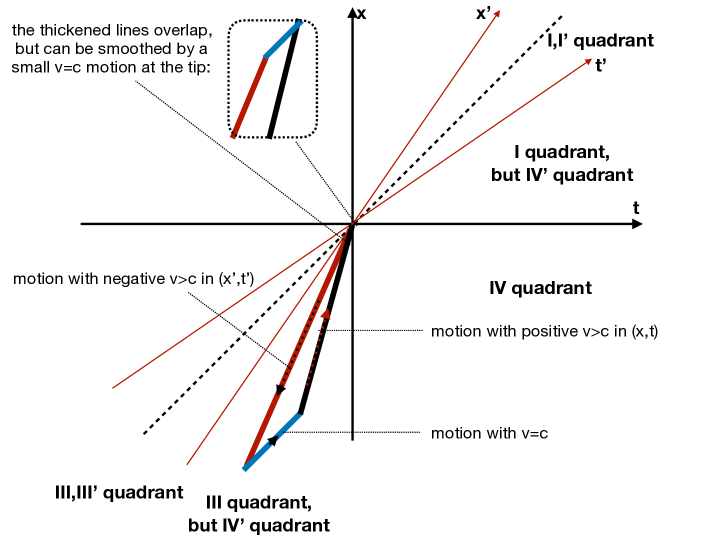
Figure 1: The closed time-like loop constructed from velocities with $v>c$ in both $(x,t)$ and $(x^{\prime},t^{\prime})$ coordinate systems.

Physically, this corresponds to moving with $v>c$ backwards in the system moving forwards ($x/t>0$), then at (close to) the speed of light forwards, then at $v>c$ forwards.

Now, in the localized curved space, we assume that the space is curved around the trajectory, so the $v>c$ lines of the loop become ”thick”, because of the gravitational field which should somehow be generated around the trajectory. But obviously, we should not have a situation where the two thicknesses touch, since then we cannot generate one field due to the presence of the other.

That seems to mean that the loop becomes impossible, since at the origin the two thicknesses could touch, but that would be easily fixed, by just adding a small line of (almost) speed of light $v=c$ motion separating the two lines. So the only way for this loop to be illegal would be if it would not be possible to generate the $v>c$ line in $(x^{\prime},t^{\prime})$ that moves backwards in $t$, since it would ”pass over” the $v>c$ line in the $(x,t)$ system in order to get from the IV quadrant to the III quadrant. But it is hard to see why this would be the case within normal general relativity. After all, the background space is Minkowski, and boosting should produce no change in the ability to construct the ”warp drive” as defined, so there is no a priori reason for it.

Example 3. FLRW space

In the case of FLRW space, as the space is not asymptotically Minkowski, it is not surprising that ”the speed of light is greater than c”, in the sense that as light passes by, the space expands, so in time $t$, light passes more than $x=t$, depending on $a(t)$. For instance, we have $x=pt=2t$ for $a(t)=t^{n}$. Of course, locally, the speed of light is still $c$, and any velocity is bounded by it, since we have local Lorentz invariance.

More importantly, in this case, there is no global Lorentz invariance, on the contrary, there is a preferred time coordinate $t$, for comoving coordinates. The corresponding system of coordinates, called sometimes the CMBR system, can be experimentally detected: we know precisely the speed of motion of the Earth and Sun with respect to this system of coordinates, i.e., with respect to the CMBR.

Formally, this global Lorentz violation is defined, as in the case of Galilean space, by the presence of a constant Lorentz vector $V_{\mu}=(1,0,0,0)$ that defines the time coordinate, leading to the FLRW metric (assuming $k=0$, i.e., flat spatial Universe)

$$ds^{2}=-dt^{2}+a^{2}(t)(dr^{2}+r^{2}d\Omega_{2}^{2}).$$ (4.6)

Of course, this Lorentz violation doesn’t help to travel with $v>c$ along some trajectory, since we can only travel at most at $v=p$, but moreover the space itself recedes away from us at the same rate, so that doesn’t help at all.

Example 4 (solution). FLRW space + special vector + curved space

Finally we arrive at the solution that I propose. We consider an FLRW spacetime solution in the theory with two times described before, with $g_{0^{\prime}0^{\prime}}\simeq 0$ in the background. Moreover, we assume that we can construct a localized curved space, but now meaning nonzero (macroscopic) $g_{0^{\prime}0^{\prime}}$ along a particular trajectory $x^{\mu}(t)$. As we saw, this means a nonzero (approximately constant over the nontrivial region needed along the trajectory $x^{\mu}(t)$) tensor $F_{(4)0^{\prime}123}$, which is consistent with the symmetries of the FLRW metric, and is equivalent (by dualization) with a constant vector $C_{0}$, i.e., $C_{\mu}=(1,0,0,0)$ in the $(0123)$ space.

In some sense then, this proposed solution is the sum of the 3 previous examples. As such, we can think from the point of view of each of the 3 previous cases, and see how we fixed the problems with them:

• From the point of view of Galilean space, we have the now constant $C_{0}$, but only along the trajectory $x^{\mu}(t)$, thus not contradicting relativity. The existence of the FLRW metric is essential for its construction (provides the symmetries needed for constructing $C_{0}$)

• From the point of view of the localized curved space, now we have also the constant vector, which means that the two boosted frames are not equivalent, and the picture we had, of creating a $v>c$ in the boosted frame, is not possible. More precisely, we saw that by boosting with a parameter $\gamma$, the Lorentz violation in the new system, $v^{2}_{\rm max}-1$, decreases by the same factor $\gamma$.

• From the point of view of the FLRW space, now we have the localized curved space along the desired trajectory, so we can travel faster than $c$ along it, and $C_{0}$ along the trajectory means the same thing.

We now turn to the constraints imposed in order to avoid the existence of the loop at example 2.

The motion with $v>c$ in $(x,t)$ in the loop occurs for (in the limiting case, of the maximum velocity) $x/t=v_{\rm max}$. For the system to be causal, we need to not be able to create the line that goes back in time before the beginning of the $x/t=v_{\rm max}$ line, even in the extremal case when we consider motion with $\tilde{v}_{\rm max}$ on the negative $x^{\prime}$ axis. That is, we want that the line $x^{\prime}/t^{\prime}=-\tilde{v}_{\rm max}$ is either steeper than the $x/t=v_{\rm max}$ line, or in the fourth quadrant. Then we need that ($v=\tanh\beta$ is the velocity of the boost of the coordinate system)

$$\frac{x^{\prime}}{t^{\prime}} = \frac{x\cosh\beta-t\sinh\beta}{-x\sinh\beta+t\cosh\beta}=-\tilde{v}_{\rm max}\Rightarrow$$ (4.7)

$$\frac{x}{t} =\frac{v-\tilde{v}_{\rm max}}{1-v\tilde{v}_{max}}$$ (4.8)

obeys

$$\frac{x}{t}=\frac{v-\tilde{v}_{\rm max}}{1-v\tilde{v}_{max}}\geq v_{\rm max}\;\;\;{\rm OR}\;\;\;\;\leq 0.$$ (4.9)

In the second case ($\leq 0$, line in the fourth quadrant), we obtain (since $\tilde{v}_{\rm max}>1>v$, but $v\tilde{v}_{\rm max}$ can be either positive or negative)

$$\tilde{v}_{\rm max}\geq\frac{1}{v}\Rightarrow\tilde{v}^{2}_{\rm max}-1\leq\frac{1-v^{2}}{v^{2}}\Rightarrow v^{2}_{\rm max}-1\leq\frac{1}{v^{2}}.$$ (4.10)

In the first case (when $1-v\tilde{v}_{\rm max}\leq 0$, and so $v^{2}_{\rm max}\leq 1+1/v^{2}$), we obtain the condition

$$(v_{\rm max}-v)^{2}\geq(1+(1-v^{2}(v^{2}_{\rm max}-1))(1-vv_{\rm max})^{2}.$$ (4.11)

We first note that at $v\rightarrow 1$, we obtain equality, so that seems encouraging. However, at $v=1-\epsilon$, we obtain

$$(v_{\rm max}-1)^{2}+2\epsilon(v_{\rm max}-1)\geq(v_{\rm max}-1)^{2}+2\epsilon(v_{\rm max}-1)[(v_{\rm max}-1)^{2}(v_{\rm max}+1)-v_{\rm max}]\;,$$ (4.12)

which is not satisfied for any $v^{2}_{\rm max}\geq 1+1/v^{2}$. Since the velocity $v$ is an arbitrary parameter, as we can boost the embedding Minkowskian system of coordinates to any velocity, that is all we need.

For completeness however, let us consider also the case of $v\ll 1$, which means that now

$$v^{2}_{\rm max}-1\geq\frac{1}{v^{2}}\gg 1\Rightarrow vv_{\rm max}\geq 1.$$ (4.13)

In this case, we see that the inequality is satisfied if $vv_{\rm max}-1\geq 1$, so if

$$\frac{\sqrt{1+v^{2}}}{v}\leq v_{\rm max}\leq\frac{2}{v}.$$ (4.14)

That means that if $v\ll 1$, we can extend the bound on $v_{\rm max}$ to be causal to $v_{\rm max}\leq 2/v$.

What interests however is the bound obtained by minimizing over all possible $v$’s, and in that case, as we saw, we obtain (considering the most constraining case of $v\rightarrow 1$),

$$v^{2}_{\rm max}\leq 1+\frac{1}{v^{2}}\rightarrow 2\Rightarrow v_{\rm max}\leq\sqrt{2}.$$ (4.15)

This turns into a constraint on the $g_{0^{\prime}0^{\prime}}$ that can be created,

$$g_{0^{\prime}0^{\prime}}\leq 1.$$ (4.16)

It is not clear where would such a constraint come from. Perhaps it is a signal that we cannot construct a $g_{0^{\prime}0^{\prime}}>1$ with any matter VEV. We leave this for further work.

5 Fields, quantization and observations

In this section we build up the non-Lorentz violating physical implications of the model, and explore whether there are any clear experimental signatures for the model.

First, we consider the parameters of the model. Since the gravitational action is written in 5 dimensions, we have to reduce to 4 dimensions, on the compact time direction. As we said, $R_{0}$ is the parameter that replaces the fixed ratio $dt^{\prime}/dt=1$. Since the physical periodicity of $t^{\prime}$ is $2\pi R_{0}\sqrt{g_{0^{\prime}0^{\prime}}}$, we can choose $R_{0}$ and $M_{\rm Pl,5}$ to be related as $2\pi R_{0}=R_{\rm Pl,5}=M_{\rm Pl,5}^{-1}$.

From compactification of the 5 dimensional action on the second time, we obtain

$$2\pi R_{0}\sqrt{g_{0^{\prime}0^{\prime}}}=R_{\rm Pl,5}\frac{M^{2}_{\rm Pl,4}}{M^{2}_{\rm Pl,5}}\;,$$ (5.1)

and from $2\pi R_{0}=R_{\rm Pl,5}$, we find

$$g_{0^{\prime}0^{\prime}}=\left(\frac{M_{\rm Pl,4}}{M_{\rm Pl,5}}\right)^{4}.$$ (5.2)

Then it follows that we need $M_{\rm Pl,5}\gg M_{\rm Pl,4}$. For instance, with $M_{\rm Pl,5}=10^{3}M_{\rm Pl,4}$, we obtain $g_{0^{\prime}0^{\prime}}\sim 10^{-12}$.

Next, we turn to how to write fields and to quantize them in the presence of the second time.

Unlike space, time has to flow, $dt^{\prime}>0$, so for matter and its fields, we must have an $x_{0^{\prime}}$ dependence. But then, if $x_{0^{\prime}}$ is compact, it means that $e^{iE^{\prime}x_{0^{\prime}}\sqrt{g_{0^{\prime}0^{\prime}}}}$ must be single valued around the circle, which means that

$$E^{\prime}=\frac{n}{R_{0}\sqrt{g_{0^{\prime}0^{\prime}}}}$$ (5.3)

so, if it is not zero, it is very large (at the Planck scale). Then, it can be the case that $E^{\prime}=0$ for all physical processes we observe today, in which case when quantizing, we just write wavefunctions

$$e^{-iEt+i\vec{k}\cdot\vec{x}}\cdot e^{-iE^{\prime}t^{\prime}\sqrt{g_{0^{\prime}0^{\prime}}}}\rightarrow e^{-iEt+i\vec{k}\cdot\vec{x}}\;,$$ (5.4)

so everything is standard, despite the fact that $dt^{\prime}/dt=1$! That means that we don’t have to change anything in the quantization of fields for energies below the Planck scale, which is what we would have wanted for consistency anyway.

A natural question that arises in the context of a quantum theory with a second time is the question of unitarity. In the case of fields, and of being in the vacuum, as we said, we have $n=0$, so fields are not excited in the second time, and nothing changes. But in the case of excited states with $n>0$, or of usual quantum mechanics of particles, we have a legitimate question. It is beyond the scope of this paper to define a full quantum mechanical theory, but we just note that, in the special FLRW frame, it is natural to construct a Schrodinger equation in terms of time evolution in the affine parameter (“proper time” $\tau$ of eq. (3.3)), instead of the usual time $t$. In this case, unitarity works in the same way as for a single time $t$, and there is no contradiction. The question of how to construct a fully covariant quantum theory, in particular for fields, is a hard one however. It is also less obvious what to do in the case of fields with $n>0$, but the quantum mechanical case suggests that, at least in the FLRW frame, viewing the field as a collection of particles leads to no problems with unitarity, since the times $t$ and $t^{\prime}$ flow together for these particles, and one just has to be careful to define probabilities and their evolution with respect to the evolution in $\tau$, not $t$.

One assumption about our model was based on the quantization of matter fields: we assumed that we can vary $m$, as the VEV of some matter fields, like some function of the Higgs scalar, or a fermion bilinear getting a VEV, or $\mathop{\rm Tr}\nolimits[F_{\mu\nu}F^{\mu\nu}]$. Specifically, we want

$$m=[\langle\bar{\psi}\psi\rangle]^{1/3}\;\;\;{\rm or}\;\;\;\left(\mathop{\rm Tr}\nolimits[F_{\mu\nu}F^{\mu\nu}]\right)^{1/4}\;\;\;{\rm or}\;\;\;\left[|H|^{2}\right]^{1/2}.$$ (5.5)

Observations

Besides directly activating the second time, i.e., increasing $g_{0^{\prime}0^{\prime}}$ as shown in the rest of the paper, the same lack of new phenomena below the Planck scale that we just mentioned also means that it is hard to pinpoint a smoking gun for the model. One could observe the presence of an infinitesimal $F_{0^{\prime}123}$ perhaps, just that we chose it for the reason that it is consistent with the CMBR, so it would be hard to disentangle experimentally from it. We mentioned that $m$ must appear from some VEVs of matter fields, but normally it has to be infinitesimal too, so that is also difficult to observe.

The one remaining possibility involves the field $\lambda$. If it is a Lagrange multiplier, there is nothing to observe, but if it is dynamical, there is a chance. The first observation is that $\partial_{0^{\prime}}\lambda=0$ if $E^{\prime}=0$, even though in its kinetic term, we have $(\partial_{0^{\prime}}\lambda)^{2}g^{0^{\prime}0^{\prime}}$, with $g^{0^{\prime}0^{\prime}}\simeq 1/g_{0^{\prime}0^{\prime}}\gg 1$. So we cannot observe directly the second time through it either.

However, in this model, we have the quantum process $\lambda\rightarrow\phi\phi$, or rather, $\lambda\rightarrow A_{(3)0^{\prime}12}A_{(3)0^{\prime}12}$, and perhaps $\lambda$ can be identified with the Higgs. If we consider $\phi$ as the field, a scalar decaying in two other scalars is not much of a smoking gun, but as we saw, in the presence of gravity, the scalar and 3-form behave differently. If one could experimentally decide that the decay is really into two 3-forms, and not two scalars, then we would have a better test of the model.

6 Conclusions

In this paper I have shown that, if we consider the possibility of a small compact second time coordinate, under certain conditions we can have super-luminal propagation that is both causal, and respects general coordinate invariance. One needs a specific model, where a fundamental totally antisymmetric 3-form field $A_{(3)MNP}$ can get a nonzero field strength $F_{(4)0^{\prime}123}$ via a coupling to the VEV $m$ of some matter fields, assumed to be possible to vary. In turn, $F_{(4)0^{\prime}123}$, consistent with the FLRW Universe, can increase $g_{0^{\prime}0^{\prime}}$, increasing the physical (effective) radius of the second time. Motivating 4 physical principles (from the physics that we should observe from them) related to the presence of the second time, I derived from them that we have an apparent Lorentz violation of $v^{2}_{\rm max}-1=g_{0^{\prime}0^{\prime}}/\gamma^{2}$, that is causal, at least for $v_{\rm max}\leq\sqrt{2}$, since $\gamma$ refers to the boost away from the FLRW cosmic time reference system.

It should be noted that I have only proved that if we can construct (enhance) a macroscopic $g_{0^{\prime}0^{\prime}}$ around the (super-luminal) trajectory of a macroscopic object (”spaceship”), then we obtain the causal apparent Lorentz violation $v^{2}_{\rm max}-1$ from the point of view of the observer far away (i.e., ”on Earth”). The issue of how to actually construct this $g_{0^{\prime}0^{\prime}}$ (via increasing the VEV $m$ of matter fields) around the trajectory was not discussed. Therefore the present paper must be understood as a proof of principle of the possibility of causal super-luminal macroscopic propagation in the presence of the second time coordinate, and not as a way to actually construct such propagation.

References

- [1] M. Alcubierre, “The Warp drive: Hyperfast travel within general relativity,” Class. Quant. Grav. 11 (1994) L73–L77, arXiv:gr-qc/0009013 [gr-qc].
- [2] M. S. Morris and K. S. Thorne, “Wormholes in space-time and their use for interstellar travel: A tool for teaching general relativity,” Am. J. Phys. 56 (1988) 395–412.
- [3] B. Elder, A. Joyce, and J. Khoury, “From Satisfying to Violating the Null Energy Condition,” Phys. Rev. D89 (2014) no. 4, 044027, arXiv:1311.5889 [hep-th].
- [4] I. T. Drummond and S. J. Hathrell, “QED Vacuum Polarization in a Background Gravitational Field and Its Effect on the Velocity of Photons,” Phys. Rev. D22 (1980) 343.
- [5] I. Bars and C. Kounnas, “Theories with two times,” Phys. Lett. B402 (1997) 25–32, arXiv:hep-th/9703060 [hep-th].
- [6] I. Bars and C. Kounnas, “String and particle with two times,” Phys. Rev. D56 (1997) 3664–3671, arXiv:hep-th/9705205 [hep-th].
- [7] I. Bars, C. Deliduman, and D. Minic, “Supersymmetric two time physics,” Phys. Rev. D59 (1999) 125004, arXiv:hep-th/9812161 [hep-th].
- [8] I. Bars, “Two time physics in field theory,” Phys. Rev. D62 (2000) 046007, arXiv:hep-th/0003100 [hep-th].
- [9] I. Bars, “Survey of two time physics,” Class. Quant. Grav. 18 (2001) 3113–3130, arXiv:hep-th/0008164 [hep-th]. [,333(2000)].
- [10] H. Nastase, “Constant H field, cosmology and faster than light solitons,” arXiv:hep-th/0601182 [hep-th].