Polaron mobility in the “beyond quasiparticles” regime

Abstract

In a number of physical situations, from polarons to Dirac liquids and to non-Fermi liquids, one encounters the “beyond quasiparticles” regime, in which the inelastic scattering rate exceeds the thermal energy of quasiparticles. Transport in this regime cannot be described by the kinetic equation. We employ the Diagrammatic Monte Carlo method to study the mobility of a Fröhlich polaron in this regime and discover a number of non-perturbative effects: a strong violation of the Mott-Ioffe-Regel criterion at intermediate and strong couplings, a mobility minimum at $T\sim\Omega$ in the strong-coupling limit ($\Omega$ is the optical mode frequency), a substantial delay in the onset of an exponential dependence of the mobility for $T<\Omega$ at intermediate coupling, and complete smearing of the Drude peak at strong coupling. These effects should be taken into account when interpreting mobility data in materials with strong electron-phonon coupling.

Mobility of non-degenerate charge carriers in ionic semiconductors with strong electron-phonon coupling is a long-standing problem Low ; LK ; Alexandrov . Textbook treatment starts with the notion of a transport scattering time $\tau$ controlling momentum relaxation in the equation of motion $\dot{{\mathbf{p}}}={\mathbf{E}}-{\mathbf{p}}/\tau$, where ${\mathbf{E}}$ is the external electric field (we set $e=1$, $\hbar=1$, and $k_{B}=1$, for brevity). The underlying assumption is that all effects originating from coupling the particle to its environment (in this work we consider a single particle coupled to a translationally-invariant bath) are reduced to an effective friction force. The equation of motion leads to a familiar result for the frequency-dependent Drude mobility,

$$\mu(\omega)=\frac{\tau/M}{1-i\omega\tau}\;,$$ (1)

with $M$ being the bare particle mass.

Deducing the scattering time from the DC mobility by using $\tau=\mu(0)M\equiv\mu M$ faces a problem because coupling to the environment necessarily leads to mass renormalization, $M\to M^{*}$. One might argue that substituting $M^{*}$ instead of $M$ into Eq. (1) would solve the issue. However, this procedure implicitly assumes that $M^{*}$ can be measured or calculated separately in a setup where particles propagate coherently and relaxation processes can be neglected at the relevant energy scales. In other words, one has to require that $E\tau(E,T)\gg 1$ (in general, $\tau$ may depend on the particle energy, $E$), or

$$\tau(T)\gg 1/T\;,$$ (2)

if $E$ is replaced with the typical thermal energy $(d/2)T$, with $d$ being the spatial dimension. Here, $\tau(T)$ should be understood as the inelastic scattering time. For elastic scattering, either by impurities or phonons above the Bloch-Grüneisen temperature, condition (2) is not relevant physkin . Likewise, it can be strongly violated in lattice models in the hopping mobility regime Holstein59 ; minimum when the local rather than momentum representation is more adequate. Condition (2) can be reformulated as $\ell\gg\lambda_{T}$, where $\ell$ is the mean free path and $\lambda_{T}$ is the particle de Broglie wavelength. In this form, it coincides with the “thermal” version of the Mott-Ioffe-Regel (MIR) criterion for the validity of the kinetic equation approach, which has attracted a lot of attention recently in the context of bad and strange metals hartnoll_book ; hartnoll ; bruin .

In this Letter, we analyze the violation of the MIR criterion for a tractable yet non-trivial system, namely the Fröhlich polaron model Frohlich . Apart from being a canonical polaron problem Landau ; Appel , it plays the main role in understanding charge transport in ionic semiconductors. It is described by the Hamiltonian $H=H_{\rm e}+H_{\rm ph}+H_{\rm e-ph}$ where

$$H_{\rm e}=\sum_{\mathbf{k}}\frac{k^{2}}{2M}\,c_{\mathbf{k}}^{\dagger}c_{\mathbf{k}}^{\,}\;,\;\;\;\;H_{\rm ph}=\sum_{\mathbf{q}}\Omega\,b_{\mathbf{q}}^{\dagger}b_{\mathbf{q}}^{\,},$$ (3)

$$H_{\rm e-ph}=\sum_{{\mathbf{k}},{\mathbf{q}}}V({\mathbf{q}})\,(b_{\mathbf{q}}^{\dagger}-b_{-\mathbf{q}}^{\,})\,c_{{\mathbf{k}}-{\mathbf{q}}}^{\dagger}c_{\mathbf{k}}^{\,}\;,$$ (4)

with $V({\mathbf{q}})=i\sqrt{2^{3/2}\pi\Omega^{3/2}\alpha/M^{1/2}q^{2}}$. Coupling between electrons and optical phonons with energy $\Omega$ can no longer be assumed weak when the dimensionless constant $\alpha>1$. Perturbation theory predicts that the polaron $Z$-factor in the ground state is given by $Z=1-\alpha/2$ to leading order. As revealed by stochastically exact Diagrammatic Monte Carlo (diagMC) simulations us1 ; us2 , the actual $Z$-factor is about $0.3$ already at $\alpha=2$ and drops down to $\approx 0.01$ at $\alpha=6$.

As far as the Fröhlich polaron mobility at finite temperature is concerned, rigorous analytical results can only be obtained within some version of perturbation theory, based either on weak coupling or the Migdal theorem. In the anti-adiabatic regime ($T\ll\Omega$), one can only rely on weak coupling ($\alpha\ll 1$). This limit was considered by Kadanoff and Langreth LK , who calculated all diagrams for $\mu$ up to order ${\cal O}(1/\alpha)+{\cal O}(1)$ with the result

$$\mu=\frac{e^{\Omega/T}}{2M^{*}\alpha\Omega}=\frac{1/\alpha-1/6}{2M\Omega}e^{\Omega/T}\,,\;\;\;(T\ll\Omega,\alpha\ll 1)\;,$$ (5)

The ${\cal O}(1)$ correction accounts for effective mass renormalization, $M^{*}=M/(1-\alpha/6)$, and is legitimate. There is also a number of variational results; a widely used one is the Low and Pines formula Low , which has the same form as (5) with $M^{*}=M(1+\alpha/6)^{3}/f(\alpha)$, where $f(\alpha)\approx 5/4$ for $3<\alpha<6$. In the adiabatic limit ($T\gg\Omega$), one can neglect vertex corrections when computing the scattering rate and find the mobility from the kinetic equation, whose solution is radically simplified by the fact that scattering is quasi-elastic. The result is a mobility that slowly decreases with $T$ Supplemental ,

$$\mu=\frac{4}{3\sqrt{\pi}\alpha M\sqrt{\Omega T}}\;\;\;\;\;(T\gg\Omega)\,.$$ (6)

The $1/\sqrt{T}$ scaling of $\mu$ is a combination of the $T$ scaling of the phonon occupation numbers and the $\sqrt{T}$ scaling of the thermal velocity. In contrast to Eq. (5), $\alpha$ is not is not required to be small for Eq. (6) to be valid.

For $\alpha\gg 1$ both limits predict that at $T\sim\Omega$ one enters the “beyond quasiparticles” regime, in which $\tau(T)$ –defined as $M\mu(T)$– is shorter than the Planckian bound. As far as we know, the mobility of Fröhlich polarons has never been computed with controlled accuracy in this parameter regime.

In this Letter, we address this unsolved problem by extending the diagMC method us1 ; us2 to finite temperatures in combination with analytic continuation methods us2 ; us3 ; tutorialtext and computing the mobility from the Matsubara current-current correlation function. We find that for $\alpha>1$ the MIR condition, formulated as $\mu\gg 1/MT$, is indeed violated. Contrary to expectations based on perturbation theory, the exponential increase of the mobility with decreasing temperature, Eq. (5), is observed only at temperatures significantly below $\Omega$. Even more surprising is a mobility minimum developing at $T\sim\Omega$ for large values of $\alpha$. We interpret both effects as a competition between the decreasing number of thermal excitations and a strong enhancement of the polaron mass, both of which taking place as temperature is lowered.

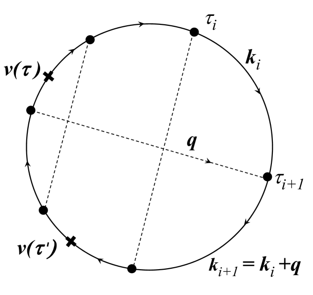
Figure 1: A typical Feynman diagram contributing to the current-current correlation function. Solid (dashed) lines stand for electron (phonon) propagators $G$ ($D$), dots are representing interaction vertices $|V|$, and crosses mark velocity measurements.

Method. As far as the diagMC method is concerned, our finite temperature calculation (in which we used the units $M=\Omega=1$) is similar to that employed for calculating the optical conductivity in Ref. us4 for $T=\beta^{-1}\to 0$. The difference is that now phonon propagators in imaginary time are temperature dependent, $D(\tau)=[e^{-\Omega\tau}+e^{\Omega\tau-\Omega\beta}]/[1-e^{-\Omega\beta}]$, and we do not assume that $e^{-\Omega\beta}$ is small. A typical diagram contributing to the current-current correlation function $C(\tau-\tau^{\prime})=d^{-1}\langle{\mathbf{v}}(\tau){\mathbf{v}}(\tau^{\prime})\rangle\equiv(dM^{2})^{-1}\langle{\mathbf{k}}(\tau){\mathbf{k}}(\tau^{\prime})\rangle$ is shown in Fig. 1. By using Matsubara frequencies, $\omega_{m}=2\pi mT$ (with $m$ integer), we obtain an efficient unbiased Monte Carlo estimator for its Fourier transform,

$$C_{m}=\int_{0}^{\beta}d\tau C(\tau)\,e^{i\omega_{m}\tau}\equiv\frac{1}{d\beta M^{2}}\langle|{\mathbf{k}}_{m}|^{2}\rangle.$$ (7)

The value of ${\mathbf{k}}_{m}$ for a diagram of order $N$ is readily found from the electron momenta $\{{\mathbf{k}}_{i}\}$ in imaginary time intervals $i=1,\dots,2N$ ranging from $\tau_{i}$ to $\tau_{i+1}$ (cf. Fig 1),

$${\mathbf{k}}_{m}=\int_{0}^{\beta}d\tau{\mathbf{k}}(\tau)\,e^{i\omega_{m}\tau}=\sum_{i}^{2N}{\mathbf{k}}_{i}\frac{e^{i\omega_{m}\tau_{i+1}}-e^{i\omega_{m}\tau_{i}}}{i\omega_{m}}\,.$$ (8)

There are several exact and asymptotic relations relations that the correlation function has to satisfy. Any of them can be used as an independent check on the accuracy of the data. For the equal-time correlator we find that $T\sum_{m}C_{m}=\langle k^{2}\rangle/dM^{2}$. The sum rule for the mobility translates into $C_{m=0}=1$. The asymptotic behavior in the limit of large $|m|$ comes from diagrams containing very short time intervals $\tau_{i+1}-\tau_{i}=\Delta\tau\to 0$ with large particle momenta $k_{i}\sim 1/\sqrt{\Delta\tau}\to\infty$. Dressing such intervals by vertex corrections is not necessary because it would result in additional factors of $\sqrt{\Delta\tau}$. Therefore, one can use perturbation theory to compute the high-frequency limit with the final result

$$C_{m\to\infty}\to\frac{2\sqrt{2}\,\alpha\coth[\Omega\beta/2]}{d\,\omega_{m}^{3/2}}\;.$$ (9)

To determine the mobility, one needs to perform the analytic continuation numerically, which amounts to inverting the Kramers-Kronig transformation

$$C_{m}=\frac{2}{\pi}\int_{0}^{\infty}d\omega\,\frac{\omega^{2}\mu(\omega)}{\omega^{2}+\omega_{m}^{2}}\;.$$ (10)

The asymptotic behavior implied by $C_{m}$ immediately yields the asymptotic behavior of $\mu(\omega)$

$$\mu(\omega\to\infty)\to\frac{2\alpha\coth[\Omega\beta/2]}{d\,\omega^{5/2}}\;,$$

which can be used to subtract the leading tail contribution when performing the analytic continuation. The nature of Eq. (10) is such that even tiny error bars on $C_{m}$ translate into large uncertainties on integrals of $\mu(\omega)$ over physically relevant intervals. All errors on the $\mu(\omega)$ function itself are conditional and depend on constraints for allowed behavior us3 . In this work, Monte Carlo data for the lowest Matsubara frequencies were accurate at the level of five to six significant digits.

Our analytic continuation method for solving Eq. (10) is similar to the one used in Ref. minimum . The main difference is that we extract $\mu(\omega)$ from the data parameterized by the Matsubara frequency rather than imaginary time. We also employ more conservative protocols for computing both the mobility and its errorbars from multiple solutions of the stochastic optimization with the consistent constraints method (see Supplemental material) us2 ; us3 .

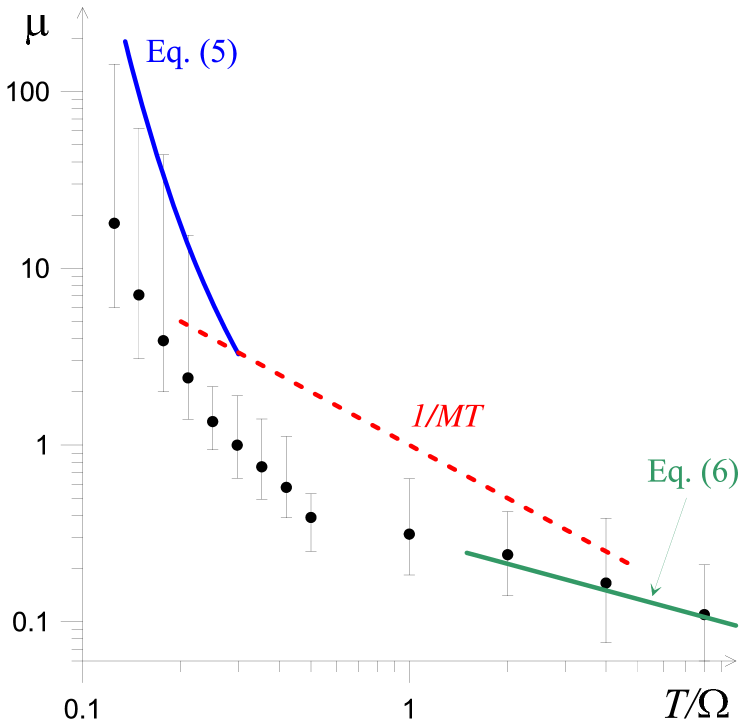
Figure 2: (color online). Black dots: mobility of a Fröhlich polaron as a function of temperature at intermediate coupling ($\alpha=2.5$). Blue and green lines are predictions based on Eqs. (5) and (6), respectively. Below the dashed red line, $\mu=1/MT$, the MIR criterion is violated.

Results. To begin with, we verified that our results for the mobility are consistent with the predictions (5) and (6) based on perturbation theory for small $\alpha=0.25$. In this case, the MIR criterion is not violated even at $T\sim\Omega$, i.e., the mobility remains large compared to $1/MT$. When the coupling strength is increased to $\alpha=2.5$, the situation changes. As Fig. 2 shows, the MIR criterion is violated over a broad temperature interval $0.2<T/\Omega<10$. The data for $T>\Omega$ approach the limiting form in Eq. (6), as expected, because Eq. (6) is valid for any $\alpha$. On the other hand, one should not expect the low-temperature formula (5) to be valid beyond weak coupling. Indeed, it is clear from Fig. 2 that the slow temperature dependence extends down to at least $T\sim\Omega/2$. At lower temperatures, our data are consistent with the exponential increase of the mobility, but uncertainties amplified by the analytic continuation procedure become too large for a meaningful analysis.

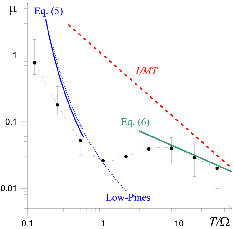
Figure 3: (color online). Mobility of a Fröhlich polaron as a function of temperature at strong coupling ($\alpha=6$). All notations are identical to those in Fig. 2. Eq. (5) is plotted using the exact result $M^{*}=7.3$ instead of its perturbative approximation; otherwise the curve would go unphysical. The Low-Pines formula Low is shown by a dotted line comment_LP .

A delay (at $T<\Omega$) in the onset of the exponential dependence may be anticipated already from perturbation theory. Indeed, matching Eqs. (5) and (6), we find that the crossover temperature

$$T_{\text{cr}}\sim\frac{\Omega}{\ln\lambda}\left(1-\frac{\ln\ln\lambda}{2\ln\lambda}+\dots\right)$$ (11)

with $\lambda\equiv M^{*}/M$ is (logarithmically) suppressed compared to $\Omega$ for $\lambda\gg 1$.

One might argue that the MIR criterion cannot be specified down to a well-defined numerical factor and, thus, having $\mu MT=1/4$ for $\alpha=2.5$ is merely a borderline situation. However, the strong coupling case ($\alpha=6$) (cf. Fig. 3) shows that there is no obvious limit on how small the value of $\mu MT$ can be. Even more surprising is the finding that the mobility develops a minimum at $T/\Omega\lesssim 1$ and that the high-temperature limit is recovered only after a maximum at $T/\Omega\sim\alpha$, see Fig. 3. The $\mu MT$ value at the minimum is about $1/30$.

The mobility minimum for lattice polarons is a well-established phenomenon (see, e.g., Refs. Holstein59 ; Friedman63 ; minimum ; minimum1 ; minimum2 ), known as “activated hopping” between lattice sites. However, we are not aware of any work on the mobility minimum for Fröhlich polarons because the notion of hopping is ill-defined in the continuum. To understand the origin of the non-monotonic behavior, we note that for $\alpha=6$ the effective mass renormalization at low temperatures and small momenta is very strong, $M^{*}/M\approx 7.3$ us2 , while the physics at high temperatures is still captured by the Migdal theorem. The mobility minimum then emerges from the competition between the decreasing number of thermal excitations and the strong particle mass renormalization: The former dominates at $T/\Omega\ll 1$, while the latter is more important at $T/\Omega\gtrsim 1$.

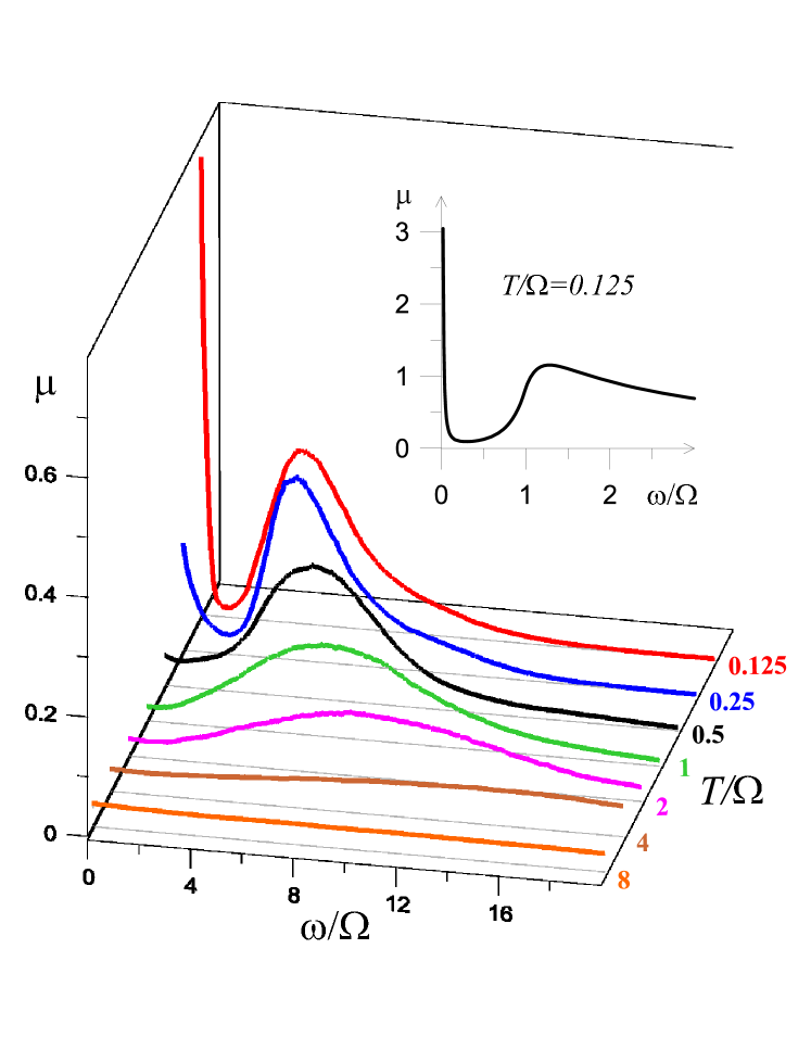
Figure 4: (color online). The real part of the mobility for $\alpha=6$ as a function of frequency at different temperatures. At low temperatures (red and blue curves) we observe a well-defined Drude peak. In the temperature interval $0.5\leq T/\Omega\leq 4$ the mobility has a local minimum at $\omega=0$ that cannot be explained within the kinetic-equation approach. Only at $T/\Omega=8$ the situation changes back to having a (barely visible) broad maximum at $\omega=0$. For comparison, the inset displays the real of part of the mobility for a Holstein polaron at weak coupling Supplemental .

If renormalization of the effective mass, which is temperature and energy dependent, does play such an important role, then the dependence of $\mu$ on $\omega$ should be radically different from the prediction of the Drude model in Eq. (1). To check this assertion we present the real part of $\mu(\omega,T)$ in Fig. 4. At the two lowest temperatures ($T=0.125\,\Omega$ and $T=0.25\,\Omega$), $\mu(\omega,T)$ exhibits a narrow Drude peak at low frequencies and a broad maximum at intermediate frequencies. In the context of small lattice polarons, the broad maximum in the mobility is commonly attributed to ionization of bound states Emin . In a broader context, however, this maximum is referred to as “Holstein band” and arises because emission of phonons is activated for $\omega$ above the characteristic phonon frequency Allen ; Timusk . The Fröhlich model is just one example; another one is the Holstein model the result for which is shown in the inset in Fig. 4.

For $T/\Omega\gtrsim 0.5$ the Drude peak in the mobility disappears. Moreover, for $T/\Omega\gtrsim 2.0$ the broad maximum becomes barely distinguishable. Any attempt to extract the scattering time from the frequency dependence of the mobility obviously fails in this regime. Our interpretation instead is to use the physically appealing relation $\tau^{-1}\sim E\sim T$ in order to conclude that the effective mass defined through $M^{*}\sim\tau/\mu$ undergoes strong renormalization as the temperature is lowered down to $T<\Omega$ (which is further confirmed by calculating the effective mass at $T=0$).

Even if the mobility retains a Drude peak but the MIR criterion is violated, the scattering time can not be extracted from the Drude formula. This is supported by an example of a heavy particle with a large transport scattering cross-section embedded into a Fermi sea, e.g., an electron bubble in ³He. Its mobility is described by Eq. (1), cast in the form $\mu(\omega)=1/M(\Gamma-i\omega)$, with a width $\Gamma\approx\text{const}$ down to temperatures exponentially lower than $\Gamma$ ionsHe3 . This result is also well known in the context of Ohmic dissipative models Schmid ; Bulgadaev . Interpreting $\Gamma$ as the scattering rate at temperatures $T\ll\Gamma$ implies that the particle mass is not renormalized. However, if the Planckian bound on the scattering rate $1/\tau(T)$ is to be obeyed, one is forced to conclude that the effective mass has to diverge as $M^{*}\propto M\Gamma/T$ in order to maintain a constant DC mobility $\mu=1/M\Gamma\sim\tau(T)/M^{*}(T)$. That the last interpretation is physically correct is revealed by considering the superfluid state at $T\ll T_{C}\ll\Gamma$, when the undamped particle motion is controlled by the strongly renormalized effective mass $M^{*}\propto M\Gamma/T_{C}$ ionsHe3 .

In conclusion, we have studied the problem of electron mobility in ionic semiconductors in the temperature regime where the MIR criterion for the applicability of the kinetic-equation approach is violated. We found that the mobility can be orders of magnitude smaller than the MIR value of $1/MT$. This result is consistent with recently observed MIR violation for non-degenerate charge carriers in doped SrTiO₃ Behnia . At strong coupling, the mobility has a minimum at a temperature comparable to the optical mode frequency and increases with a further increase of the temperature despite the fact that the number of thermally excited phonons grows linearly with $T$. We ascribe this behavior to the “undressing” of polarons at higher temperatures. After going through a maximum at $T\gg\Omega$, the mobility follows the $\mu\sim T^{-1/2}$ law predicted by the kinetic equation.

Acknowledgments. We acknowledge stimulating discussions with K. Behnia and T. Timusk. This work was initiated and partially performed at Aspen Center for Physics supported by the National Science Foundation grant PHY-1607611. We acknowledge support by the Simons Collaboration on the Many Electron Problem (N.P.), the National Science Foundation under grant DMR-1720465 (N.V.P.) and DMR-1720816 (A.K. and D.L.M.), the ImPACT Program of the Council for Science, Technology and Innovation (Cabinet Office, Government of Japan) and JST CREST Grant Number JPMJCR1874, Japan (A.S.M.), and by FP7/ERC Consolidator grant QSIMCORR No. 771891, the Nanosystems Initiative Munich and the Munich Center for Quantum Science and Technology (L.P.). Open Data for this project can be found at https://gitlab.lrz.de/QSIMCORR/mobilityfroehlich

References

- (1) F.E. Low and D. Pines, Phys. Rev. 98, 414 (1955).
- (2) L.P. Kadanoff, Phys. Rev. 130, 1364 (1963); D.C. Langreth and L.P. Kadanoff, Phys. Rev. 133, A1070 (1964).
- (3) Polarons in Advanced Materials, edited by S.A. Alexandrov, Canopus/Springer, Bristol (2007).
- (4) E. M. Lifshitz and L. P. Pitaevskii, Physical Kinetics, Course of Theoretical Physics, v. X, Butterworth-Heinemann, Burlington (1981).
- (5) A.S. Mishchenko, N. Nagaosa, G. De Filippis, A. de Candia, and V. Cataudella, Phys. Rev. Lett. 114, 146401 (2015).
- (6) T. Holstein, Ann. Phys. (N.Y.) 8, 343 (1959).
- (7) See, e.g., S. A. Hartnoll, A. Lucas, and S. Sachdev, Holographic Quantum Matter, MIT Press, Cambridge, (2018). and references therein.
- (8) S. A. Hartnoll, Nature Phys. 11, 54 (2015).
- (9) J. A. N. Bruin, H. Sakai, R. S. Perry, and A. P. Mackenzie, Science 339, 804 (2013).
- (10) H. Fröhlich, H. Pelzer, and S. Zienau, Philos. Mag. 41, 221 (1950).
- (11) L.D. Landau, Phys. Z. Sowjetunion 3, 664 (1933) [English translation: Collected Papers, Gordon and Breach, New York, (1965)].
- (12) J. Appel, in Solid State Physics Vol. 21, edited by H. Ehrenreich, F. Seitz, and D. Turnbull, Academic, New York, (1968).
- (13) N.V. Prokof’ev and B.V. Svistunov, Phys. Rev. Lett. 81, 2514 (1998).
- (14) A.S. Mishchenko, N.V. Prokof’ev, A. Sakamoto, and B.V. Svistunov, Phys. Rev. B 62, 6317 (2000).
- (15) Supplemental material.
- (16) O. Goulko, A.S. Mishchenko, L. Pollet, N. Prokof’ev, and B. Svistunov, Phys. Rev. B 95, 014102 (2017).
- (17) A. S. Mishchenko, Correlated Electrons: From Models to Materials, edited by E. Pavarini, W. Koch, F. Anders, and M. Jarrel (Forschungszentrum Julich GmbH, Julich, 2012), p. 14.1.
- (18) A.S. Mishchenko, N. Nagaosa, N.V. Prokof’ev, A. Sakamoto, and B.V. Svistunov, Phys. Rev. Lett. 91, 236401 (2003).
- (19) A popular modification of the Low-Pines formula with the exponential factor replaced by the inverse Bose function, [see, e.g., H. P. R. Frederikse and W. R. Hosler, Phys. Rev. 161, 822 (1967)], does not reproduce the correct scaling of the mobility at given by Eq. (6).
- (20) L. Friedman and T. Holstein, Ann. Phys. (N.Y.) 21, 494 (1963).
- (21) F. Ortmann, F. Bechstedt, and K. Hannewald, Phys. Rev. B 79, 235206 (2009).
- (22) F. Ortmann, F. Bechstedt, and K. Hannewald, J. Phys.: Condens. Matter 22, 465802 (2010).
- (23) See, e.g., D. Emin, Phys. Rev. B13 691 48 (1993) and references therein.
- (24) P. B. Allen, Phys. Rev. B3, 305 (1971).
- (25) D. N. Basov and T. Timusk, Rev. Mod. Phys. 77, 721 (2005).
- (26) N.V. Prokof’ev, Int. J. Mod. Phys. B7, 3327 (1993).
- (27) A. Schmid, Phys. Rev. Lett. 51, 1506 (1983).
- (28) S.A. Bulgadaev, Sov. Pys. JETP 63, 369 (1986).
- (29) X. Lin, C. W. Rischau, L. Buchauer, A. Jaoui, B. Fauqué, and K. Behnia, npj Quantum Materials 2, 41 (2017).