Stages of Reionization as Revealed by the Minkowski Functionals

Abstract

We study the evolution of the hydrogen ionization field during the epoch of reionization (EoR) using semi-numerical simulations. By calculating the Minkowski functionals (MFs) of the 21cm brightness temperature field, which provides a quantitative description of topology of the neutral and ionized regions, we find that the reionization process can be divided into five stages, each with different topological structures, corresponding to isolated ionized regions (“bubbles”); connected ionized region (“ionized fibers”) which percolate through the cosmic volume; a sponge-like configuration with intertwined neutral and ionized regions after the overlap of bubbles; connected neutral regions (“neutral fibers”) when the ionized region begin to surround the remaining neutral region; and isolated neutral regions (“islands”), before the whole space is ionized except for the rare dense clumps in galaxies and minihalos and the reionization process is completed. We use the MFs and the size statistics on the ionized or neutral regions to distinguish these different stages, and find the neutral fractions at which the transition of the different stages occur. At the later stages of reionization the neutral regions are more isolated than the ionized regions, this is the motivation for the island model description of reionization. We compare the late stage topological evolution in the island model and the bubble model, showing that in the island model the neutral fibers are more easily broken into multiple pieces due to the ionizing background.

1 introduction

The epoch of reionization (EoR) is a complex and information-rich stage in the history of our Universe, during which the first galaxies formed and the intergalactic medium (IGM) transits from neutral to ionized (e.g. Dayal & Ferrara 2018). The Lyman-$\alpha$ absorption spectra of high redshift quasars show that reionization is nearly complete at $z\approx 6$ (Fan et al., 2006), while the latest cosmic microwave background (CMB) data from the Planck satellite sets the average redshift of EoR to be $z_{re}=7.82$ (Akrami et al., 2018). Recently, the Experiment to Detect the Global Epoch of Reionization Signature (EDGES) claims to detect a strong global 21cm absorption signal at redshift $z\sim 18$ corresponding to the formation of the first luminous objects (Bowman et al., 2018), though the claimed signal is too strong to be consistent with standard cosmological model, and this result still needs further confirmation from more experiments. Besides the basic timing of reionization, however, more details about this process, such as the nature and properties of the ionizing sources and the scale and morphology of the ionization field are still very uncertain. Using the 21 cm transition of neutral hydrogen as the tracer of the neutral IGM, various experiments are built or being designed in order to detect the 21 cm signals from the EoR, including the current GMRT (Paciga et al., 2011), MWA (Tingay et al., 2013), PAPER (Parsons et al., 2010), and LOFAR (van Haarlem et al., 2013), and the upcoming HERA (DeBoer et al., 2017) and SKA-low (Maartens et al., 2015). The 21 cm power spectrum may be the most comprehensively studied statistics, and it is also probably the first statistical signal to be measured in the near future. Nevertheless, much more information is expected to be extracted from other 21 cm statistics beyond the power spectrum, as the reionization process involves various non-linear processes, and the ionization field is expected to be highly non-Gaussian. Indeed, evolutionary features in the skewness (e.g. Wyithe & Morales 2007), kurtosis (e.g. Kittiwisit et al. 2018), and bispectrum (e.g. Shimabukuro et al. 2016) of the 21 cm brightness fields, among others, have been explored.

According to our current understanding, reionization began with the formation of first stars and galaxies in high density regions, which photoionized the gas in the surrounding regions and form individual ionized bubbles. As more and more galaxies form, the bubbles grow in size and number, at some point they start to connect with each other, going through a percolation process, and eventually the ionized regions overlap with each other and most of them are connected as a whole. The remaining neutral regions are then one-by-one cut off from each other and become isolated islands. The reionization process is completed with the shrinking and disappearing of these islands.

The widely adopted “bubble model” assumed isolated-bubbles topology for the early stage of reionization (Furlanetto et al., 2004), and several semi-numerical simulation programs have been developed based on this idea (Zahn et al., 2006; Mesinger et al., 2011)). It is important to know the realm in which the isolated-bubbles topology applies, before such simulations are used for interpreting the upcoming observational data. Recently, it has been recognized that the bubble overlap happens at fairly high neutral fractions (Xu et al., 2014; Furlanetto & Oh, 2016), casting doubts on the applicable range of the models based on the idea of isolated bubbles, as its basic premise is invalid except for a very brief periods. At a later stage, when most of the space have been reionized, the neutral regions become isolated, and one could then treat them as neutral islands (Xu et al., 2014), but again we need to know the point at which the topological phase transition happened and the model based on the island picture can apply.

The two-dimensional and three-dimensional topology of the ionized regions during the EoR have been investigated in a number of researches (Gleser et al., 2006; Lee et al., 2008; Hong et al., 2014; Wang et al., 2015) (Kapahtia et al., 2018; Bag et al., 2018, 2019). While the neutral fraction, matter density and spin temperature of the hydrogen atoms may all affect the 21cm signal, Yoshiura et al. (2017) demonstrated that the MFs of the 21cm field is determined primarily by the neutral fraction, so that it provides a very powerful tool to study the topological evolution process during reionization.

Here we aim to quantify the topological structure of the 21 cm brightness field in terms of the MFs, and provide a full description of the evolutionary features of the 21 cm signal through the reionization process. Using the Minkowski functionals and the statistics of ionized and neutral regions, we try to gain an understanding of how the topology of the neutral and ionized regions evolve.

In Section 2, we briefly introduce the excursion set theory of reionization, and the semi-numerical simulations, on which our topological analysis is based. The computation of MFs is given in Section 3. The evolutionary features in the topology of the 21 cm brightness field are presented in Section 4, with each subsection dedicated to a stage of EoR. Section 5 compares the topology evolution in the 21cmFAST and the IslandFAST. We then discuss the feasibility to measure the MFs with SKA in Section 6, before summarizing the main results in Section 7.

2 Semi-numerical simulations

In order to generate the ionization field and the corresponding 21 cm brightness temperature map during reionization, we use the semi-numerical simulations of the 21cmFAST (Mesinger et al., 2011) program as well as the IslandFAST(Xu et al., 2017), which is designed to have a more accurate description at the late stage of the reionization. The semi-numerical simulations are based on the excursion set theory of structure formation (Bond et al. 1991, Lacey & Cole 1993, Zentner 2007), in which the formation of luminous objects are determined by the over-density on the corresponding mass scales, and the ionization of the region is determined by the balance of ionizing photon supply and the number of baryons to be ionized–in the presence of recombination, each baryon may also require multiple photons to keep it ionized during the time being considered. The 21cmFAST program was developed based on the “bubble model” of reionization (Furlanetto et al., 2004) which assumes an isolated-bubble topology of the ionization regions. To obtain a more accurate description of the reionization process after percolation of the ionized regions, the “island model” (Xu et al., 2014) and the corresponding semi-numerical code IslandFAST (Xu et al., 2017) were developed, assuming a topology of isolated neutral islands in the ionization field. Strictly speaking, the “bubble model” should be applied only before the connection of individual bubbles, while the “island model” should be used only after the isolation of the neutral patches, and during the mid-stage of reionization when the percolation occurs, neither of these model is completely accurate. Within the framework of the excursion set theory, the watershed happens when the density barrier crosses the coordinate origin on the $\delta-S$ plane.

Although the ionized bubbles are isolated only at the early stage of reionization, it was found that the statistical predictions from the 21cmFAST still have a reasonable agreement with full radiative transfer hydrodynamical simulations for most epochs during reionization (Zahn et al., 2006). In this paper we will use the 21cmFAST to simulate the whole process of reionization, and analyze the topology of reionization. Using the MFs, we will identify the point at which neutral regions are divided into discrete pieces, after that the neutral island gives a better description of the hydrogen distribution. For the late stage, we also perform the IslandFAST simulation, which begin with an initial state generated with 21cmFAST, but then evolve the reionization sequence using the IslandFAST rules.

We assume an ionizing efficiency parameter of $\zeta=20$, and a minimum virial temperature of $10^{4}$ K for halos hosting ionizing sources as our fiducial model. For the IslandFAST, an empirical model for the ionizing background is adopted, based on the observed number density of Lyman limit systems near redshift 6 (Songaila & Cowie, 2010). The simulation box has comoving length of 1 Gpc on a side and $500^{3}$ cubic cells.

The EoR experiments measure the 21 cm brightness temperature, given by (e.g. Furlanetto et al. 2006):

$$T_{b}(z) \approx 27x_{\rm HI}(1+\delta_{m})\left(\frac{H}{{\rm d}v_{r}/{\rm d}r+H}\right)\left(1-\frac{T_{\gamma}}{T_{\rm S}}\right)$$ (1)

$$\left(\frac{1+z}{10}\frac{0.15}{\Omega_{m}h^{2}}\right)^{1/2}\left(\frac{\Omega_{b}h^{2}}{0.023}\right)[{\rm mK}],$$

where $H$ is the Hubble parameter, $\Omega_{m}$ and $\Omega_{b}$ are the matter and baryon density parameters respectively, $T_{\gamma}$ is the CMB temperature and ${\rm d}v_{r}/{\rm d}r$ is the radial gradient of the peculiar velocity. The topology of $T_{b}$ contains the three-dimensional information about the neutral fraction $x_{\rm HI}$, matter overdensity $\delta_{m}$, spin temperature $T_{\rm S}$, as well as the radio velocity gradient. The spin temperature is an weighted average of the gas kinetic temperature and the CMB temperature. At the cosmic dawn, when the first stars and galaxies formed, the spin temperature might be driven below the CMB temperature by the Wouthuysen-Field mechanism of the Lyman-$\alpha$ photons, producing an absorption trough (Chen & Miralda-Escude, 2004). However, for the major part of the epoch of reionization, especially when the ionization fraction became significant, the gas would have already been heated well above the CMB temperature, thus the tomographic signal would be found 21cm emission. Below for simplicity we assume $T_{\rm S}\gg T_{\gamma}$ in the analysis. While the density fluctuations also contribute to $T_{b}$ fluctuations, the ionization can set the brightness directly to 0. Therefore, the features in the MFs of $T_{b}$ during reionization are dominated by the $x_{\rm HI}$ distribution (Yoshiura et al., 2017). We will focus on the topology of $T_{b}=0$ contours.

3 Minkowski Functionals

To quantify the morphological structure of the reionization, we calculate the MFs (Minkowski, 1903) of the $T_{b}$ field, for which there are only four independent ones in three dimensional space (Schmalzing & Buchert, 1997). A typical set of MFs in the three dimensional space is:

$$V_{0}(\nu)=\frac{1}{V}\int_{V}{\rm d}^{3}x~{}\Theta[u(\mathbf{x})-\nu\sigma]$$ (2)

$$V_{1}(\nu)=\frac{1}{6V}\int_{\partial F_{\nu}}ds$$ (3)

$$V_{2}(\nu)=\frac{1}{6\pi V}\int_{\partial F_{\nu}}{\rm d}s~{}[\kappa_{1}(\mathbf{x})+\kappa_{2}(\mathbf{x})]$$ (4)

$$V_{3}(\nu)=\frac{1}{4\pi V}\int_{\partial F_{\nu}}{\rm d}s~{}\kappa_{1}(\mathbf{x})\kappa_{2}(\mathbf{x})$$ (5)

where $\Theta$ denotes the Heaviside step function, $u(\mathbf{x})$ is the random field being studied, $\sigma$ is the root mean square (rms) of the field, and $\nu=u_{\rm thr}/\sigma$ is the relative threshold. $V$ denotes the three dimensional space being studied, $x$ denotes the comoving coordinates, $\partial F_{\nu}$ denotes the contour surface formed by $u(\vec{x})=\bar{u}+\nu\sigma$, $\kappa_{1,2}$ are the principle curvatures of $\partial F_{\nu}$. These MFs, in order, describes the volume, surface area, mean curvature and the Gaussian curvature of the excursion sets, i.e. regions in which the field $u$ exceeds certain threshold. By the Gaussian integration theorem, $V_{3}$ is also the Euler characteristic, which is related to the genus by $g=1-\chi/2$, which describes the topology of the excursion set, with $gV$ = (number of tunnels) - (number of isolated surfaces)+1.

We smooth the $T_{b}$ field with the simple average and a smoothing scale of $4^{3}$ cells (8 Mpc a side). The 21cm fluctuation $T_{b}/\sigma_{T_{b}}$ is used as the probe field, and as we discussed above, the $T_{b}=0$ contours trace the ionization fronts. During the reionization, at least in popular reionization models with soft ionizing photon sources, the boundary between the ionized regions and neutral regions are sharply defined. At such boundary $T_{b}=0$, thus we may watch for the $T_{b}=0$ point in the MF for the evolution of ionized regions. Other points in the MFs reflect also the change in the density of the neutral hydrogen field, though being affected by many factors it is more difficult to interpret.

We use the Koenderink method (Koenderink, 1984) to calculate the MFs. This method obtain the principal curvature by calculating the first and second order partial derivatives of the field, and transforms the surface integrals to volume integrals for computation using the Gaussian theorem.

Before moving on to measuring the simulation results, we first consider the case of random Gaussian field, which gives a good description of primordial density field of the large scale structure in the standard cosmology model. The analytical form of the MFs are known in this case:

$$V_{0} = \frac{1}{2}-\frac{1}{2}\Phi(\frac{\nu}{\sqrt{2}})$$ (6)

$$V_{1} = \frac{2}{3}\frac{\lambda}{\sqrt{2\pi}}e^{-\nu^{2}/2}$$ (7)

$$V_{2} = \frac{2}{3}\frac{\lambda^{2}}{\sqrt{2\pi}}\nu e^{-\nu^{2}/2}$$ (8)

$$V_{3} = \frac{\lambda^{3}}{\sqrt{2\pi}}(\nu^{2}-1)e^{-\nu^{2}/2}$$ (9)

where $\nu=\delta/\sigma$, $\lambda=\sqrt{|\xi^{{}^{\prime\prime}}(0)|/(2\pi\xi(0))}$ where $\xi(r)$ denotes the correlation function at zero, and $\Phi(x)=\frac{2}{\sqrt{\pi}}\int_{0}^{x}dt~{}e^{-t^{2}}$ is the Gaussian error integral. We plot the MFs of a Gaussian random field in Fig. 1 for reference, and use them to check our code for numerically measuring the MFs.

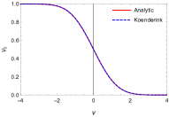
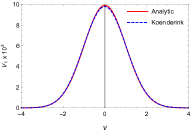
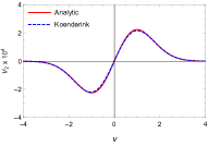
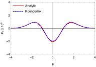
Figure 1: MFs for a Gaussian random field with $\bar{u}=0$ and $\sigma=0.5$. Red solid line denotes analytical solution and blue solid line denotes the result of numerical algorithm, which are almost identical. The resolution in this case is $128^{3}$.

We can also gain some insights on the interpretation of the MFs from this plot. The left end of the plot corresponds to extreme under-density, so the contours there would have very small total surface area ($V_{1}\sim 0$), and as the surface is oriented from high density to low density, it enclosed most of the volume ($V_{0}\sim 1$). As the density increases, the enclosed volume fraction $V_{0}$ decreases, which drops to zero at the right end for the extremely large over-density fluctuations. During the same process, the area of the contour surface $V_{1}$ initially increases as we move to more probable field values, reaching a maximum at the mean value of $\nu=0$, then starts decreasing again to smaller values at large over-densities. The mean curvature $V_{2}$ at $\nu<0$ is negative due to the orientation of the contour surface and positive at $\nu>0$, crossing zero at the mean field value of $\nu=0$. It approaches zero at large $|\nu|$, as the number and contour surface of such extreme points rapidly decrease, though the curvature itself is large. The maximum and minimum of $V_{2}$ is reached near $\nu=1$ and $-1$ respectively. However, $V_{2}$ is not frequently used in cosmological applications. The $V_{3}>0$ peaks at a moderately large $|\nu|$ indicated that $g<0$, i.e. the number of tunnels smaller than the number of isolated surfaces, while the case $V_{3}<0$ near $\nu=0$ is just the opposite, where we would have a “sponge” topology with complex multi-connected iso-density surfaces.

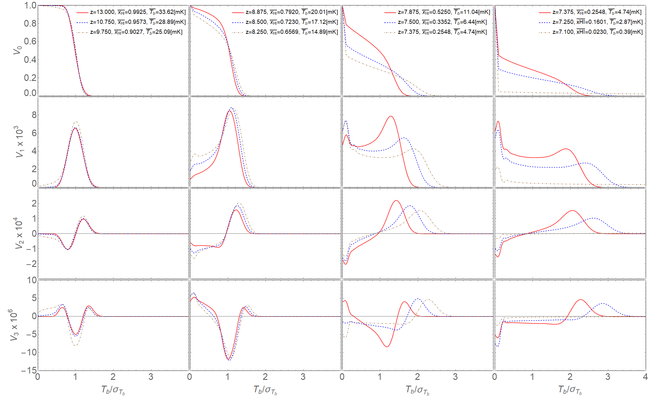
Figure 2: The Minkowski functionals at different redshifts. From top to bottom are $V_{0},V_{1},V_{2},V_{3}$ respectively, and from left to right, for each panel the MF at three redshifts (marked on the plot) are shown.

4 Stages of Reionization

In the bubble model, it is noted that the ionized bubbles first formed in high density peaks where the star formation rate is high, and as redshift decreases, more bubbles appear and existing bubbles grow in size, eventually they would overlap with each other (Furlanetto et al., 2004), then most of the space is reionized, with only a small fraction of low density regions remain as neutral islands, and afterwards they also disappeared quickly. After that, the hydrogen reionization is complete and the neutral hydrogen is only found within the high density clumps of galaxies or minihalos. However, it has been recognized recently that the percolation of the ionized bubbles could occur when the average ionized fraction is still very low (Xu et al., 2014; Furlanetto & Oh, 2016), so strictly speaking, the bona fide isolated bubble picture is only valid for a very brief period.

Armed with the MFs, we can now study the history of reionization quantitatively. However, we shall use a modified form. We shall plot the $V_{i}$ not as a function of the temperature fluctuation normalized with the variance, $\delta_{T}=(T_{b}-\bar{T_{b}})/\sigma_{T_{b}}$, but simply as a dimensionless brightness temperature $T_{b}/\sigma_{T_{b}}$. The advantage of using this is that the boundary between neutral and ionized regions have $T_{b}=0$, which we can easily mark, while in the conventional definition this point changes with $\bar{T_{b}}$.

The redshift evolution of the MFs are plotted in Fig. 2, where the MFs $V_{0},V_{1},V_{2},V_{3}$ are shown from top to bottom, the results at different redshifts are plotted on the four columns from left to right in descending order, and within each panel results for three redshifts are plotted.

Using the MFs as a classification tool, we find that the reionization history can be divided into the following five stages according to morphology:

• The Ionized Bubbles stage. Initially the MFs of the 21cm brightness temperature field are almost identical with the case of a Gaussian random field. A small number of isolated ionized bubbles begin to appear in the volume at high peaks of the density field.

• The Ionized Fibers stage. From $x_{\rm HI}\sim 0.9$ to $x_{\rm HI}\sim 0.7$, more and more bubbles get connected to form a large fiber-like structure extending the whole simulation box. While such ionized structures do not look exactly as the originally envisioned bubbles, they can still be regarded as connected bubbles embedded in the neutral box.

• The Sponge stage. When $x_{\rm HI}$ drops below 0.7, we begin to see that most of the ionized regions get connected, with the neutral and ionized regions intertwined with each to form a sponge-like complex structure.

• The Neutral Fibers stage. When the neutral fraction drops below 0.3, the neutral regions begin to look like a large fiber embedded in the ionized regions. This stage mirrors the ionized fiber stage before the sponge stage.

• The Neutral Islands stage. As reionization progresses further, the connections between the neutral regions get cut off. When $x_{\rm HI}<0.16$, the remaining large neutral regions become islands, and continue to shrink and disappear in the end.

Below, we study the evolving MFs and the stages of reionization in detail. The transition neutral fraction between each stage and the corresponding features in MFs are summarized in Table 1.

4.1 The Ionized Bubbles stage

In Fig. 2, the first column from left shows the earliest stage of the reionization process. The three curves in the figure are for redshift $z=13$ (red solid line), $z=10.75$ (blue dashed line), and $z=9.75$ (brown dash-dotted line), and the corresponding neutral fractions are $x_{\rm HI}=0.9975,0.9573,0.9025$ respectively (At the mass resolution considered here, the difference between the volume and mass-weighted neutral fractions are not large, we shall use the volume neutral fraction in all discussions in this paper.) The general impression on the MFs of this stage is that they are very close to the Gaussian case, with only minor deviations.

At the beginning of reionization ($z=13$), almost all of the gas are neutral, and the 21 cm brightness field are dominated by the density fluctuations. The MFs of the $T_{b}$ field follow those of a Gaussian field.

As the ionized bubbles formed, the neutral hydrogen field deviates from the Gaussian case. Inside the ionized regions $T_{b}=0$, and the boundary between the ionized region and neutral regions are sharp, at least for the soft ionizing sources such as stars, so we expect that the volume $V_{0}(T_{b})$ should drop steeply just above the point $T_{b}=0$, as a fraction of the volume $x_{i}=1-x_{\rm HI}$ is now ionized and has $T_{b}=0$. It should rejoin the original Gaussian curve at a height of $V_{0}=x_{\rm HI}$, if the brightness temperature field remain unchanged outside ionized region. Due to the effect of smoothing, the actual drop of $V_{0}$ is not so steep. In fact for $x_{\rm HI}\approx 0.96$ case, the difference from the Gaussian curve is very small, perhaps because the bubbles are still smaller than the smoothing scale. But we do see that for the $x_{\rm HI}\approx 0.90$ case, the $V_{0}$ decreases at $T_{b}>0$ and approaches the Gaussian curve at a value close to $x_{\rm HI}$. The same is true for the surface area $V_{1}$, which for $x_{\rm HI}\approx 0.96$ the change is unnoticeable, but for $x_{\rm HI}\approx 0.90$ the increase in $V_{1}$ is quite obvious.

The nature of the ionized region can be revealed by $V_{3}$ which is related to the topology of the field. It has an increase at $T_{b}>0$, showing an excess of contour surfaces, corresponding to the formation of bubbles. The trough of $V_{3}$ at the mean brightness temperature also deepens, perhaps due to structure growth, but this is more complicated and not relevant to the main purpose of our study, so we will not discuss it further.

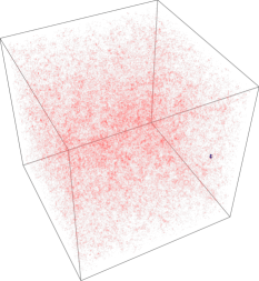
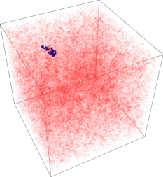
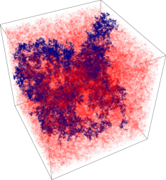
Figure 3: The largest ionized region(blue) and other ionized regions(red) at $z=13.0,x_{\rm HI}=0.9925$ (top), $z=10.75,x_{\rm HI}=0.9573$(middle), and $z=9.75,x_{\rm HI}=0.9027$ (bottom). The neutral regions are left transparent.

The simulation box at the three redshifts is shown in Fig. 3, where the ionized regions are shown in red, except the largest ionized region which is colored blue, while the neutral region are left transparent. We plot the simulation box in this way to highlight the nature of the largest ionized region. We see that at $z=13$, there are already numerous ionized bubbles, but they are all very small, so that after smoothing with a relatively large scale (8 Mpc), one would recover almost the exact Gaussian field. At $z=10.75$, the density of the ionized regions increased, and some of them merge to form large ionized regions, but even the largest ionized region is still very small. At $z=9.750$, however, even more ionized regions appear, and begin to get connected with each other to form a large ionized region. This result is consistent with the findings of Furlanetto & Oh (2016) that one large ionized bubble formed at around $\bar{x}_{\rm HI}\approx 0.9$.

The size distribution of the ionized regions at each redshift is shown in Figure 4 in units of box cells. We have made the plot such that the few largest cells appear individually as distinct spikes at the large size side in the figure. We can see that a very large ionized region appeared at $z=9.75$ box, its size exceeds other ionized regions by orders of magnitude. Such a large ionized region starts to “suppress” the growth of more ionized regions, in the sense that the newly formed ionized regions are more likely to encounter this giant one and become annexed before growing to large scale by itself. When the Universe is only $5\%$ ionized, there are still numerous ionized regions with comparable sizes of the order $10^{4}~{}V_{\rm cell}$. However, the number of these is reduced when the largest ionized region formed at $x_{\rm HI}\sim 0.9$, and the volume of other ionized regions stay much lower. The value of the distribution function at small volume is still rather large, the small bubbles are not significantly affected. Recall that due to the well known biased formation of structures, the larger bubbles are likely formed in large regions with high average density, while the many smaller bubbles are more likely to form in regions of lower average densities, so the isolated bubble assumption could still be applied to these after this stage.

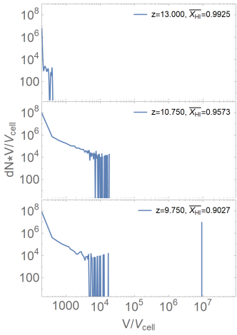
Figure 4: The size distribution of ionized regions at $z=13.000$, $\bar{x}_{\rm HI}=0.9925$ (top panel), $z=10.750$, $\bar{x}_{\rm HI}=0.9573$ (center panel) and $z=9.750$, $\bar{x}_{\rm HI}=0.9027$ (bottom panel).

4.2 The Ionized Fibers stage

The second column of Fig. 2 from left shows the MFs of the second stage of the reionization process. The three curves are for $z=8.875,x_{\rm HI}=0.792$ (red solid line), $z=8.5,x_{\rm HI}=0.7230$(blue dashed line) and $z=8.25,x_{\rm HI}=0.6569$ (brown dash-dotted line). The MFs around the ionization boundary $T_{b}=0$ are clearly different from the Gaussian field in this stage.

As noted above, at $x_{\rm HI}\sim 0.9$ a large ionized region formed, which goes through the whole simulation box. The formation of a connected ionized region which is infinitely large, or going through the whole box volume in a simulation, marks the point of percolation of ionized regions . Not all of the ionized regions are connected at this point, however, as is clearly shown in Fig. 3. But as a matter of fact, even to the very late stage of reionization, there may still be some isolated ionized regions referred to as “bubbles-in-island” in Xu et al. (2014) which are not connected. At best, one can say that most of the ionized regions get connected in this era.

After the formation of this large ionized region, as redshift decreases, more and more ionized regions get connected. The MFs near $T_{\rm b}=0$ changed appreciably. Now for $V_{0}$ the drop above $T_{b}=0$ is more apparent, and it rejoins the near-Gaussian case at $V_{0}\sim x_{\rm HI}$ as we discussed earlier. The surface area $V_{1}$ at $T_{\rm b}=0$ contours increase continuously, as ionized regions of large size formed. An additional local peak near $T_{b}\sim 0$ appeared when the global neutral fraction reaches $x_{\rm HI}\sim 0.70$. Meanwhile, the trough in the mean curvature $V_{2}$ and the peak in the Euler characteristic $V_{3}$ shifts toward left, also reaching $T_{b}\sim 0$ at $x_{\rm HI}\sim 0.70$. The position of these peaks and trough are slightly above $T_{b}=0$ thanks to the smoothing effect. These features in $V_{1},V_{2}$ and $V_{3}$ near $T_{b}=0$ indicates that there is a very large area and complicated topology and morphology for the ionized region, which is an nature outcome of the connection of the ionized regions. We shall refer to this point as the overlap of ionized regions.

As discussed in last subsection, the largest region which now permeates much of the volume has the effect of annexing the other large ionized regions. The size distribution of ionized regions is shown in Fig.5. The few largest ionized regions of $\sim 10^{4}~{}V_{\rm cell}$ in Fig. 4 now disappears, as most of the ionized regions get connected with each other. However, the number of small bubbles remain numerous, showing that not all ionized regions are connected.

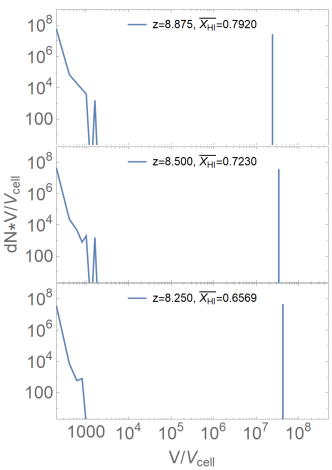
Figure 5: The size distribution of the ionized regions at $z=9.75,x_{\rm HI}=0.90275$ (top), $z=8.5,x_{\rm HI}=0.723$ (middle) and $z=8.25,x_{\rm HI}=0.6569$ (bottom).

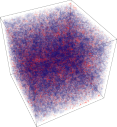
Figure 6: The largest connected ionized region at $z=8.25$.

We show the largest ionized region after the overlap of ionized regions in Figure 6. It is difficult to identify the beginning of overlap visually, but the additional peak in the Minkowski Functional $V_{1}$ curve at around $T_{b}=0$ give a cue for its occurrence. The typical global neutral fraction at which overlap happens is found to be $\bar{x}_{\rm HI}\sim 0.70$, which is consistent with the findings of Furlanetto & Oh (2016) and Bag et al. (2018).

4.3 The Sponge Stage

The MFs during next stage of reionization is shown in the third column from left in Fig. 2. Here all three curves are from an epoch after the overlap, for $z=7.875,x_{\rm HI}=0.525$ (red solid line), $z=7.5,x_{\rm HI}=0.3352$ (blue dashed line), and $z=7.375,x_{\rm HI}=0.2548$.

After the point of overlap, the whole box consists one large ionized region with small neutral regions inside, and one large neutral region, with small ionized regions inside. The two are intertwining with each other in a sponge-like morphology, as shown in Figure 7.

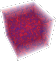
Figure 7: The largest ionized region(red) and the largest neutral region(blue) at $z=7.875$.

The evolution of the topological structure is best shown with the Euler characteristics $V_{3}$. The Euler characteristics can tell the difference between a solid sphere in an empty space, which has a positive $\chi$, and holes inside a solid object, which has a negative $\chi$. The Euler characteristics is additive, so whether the $V_{3}$ value is positive or negative can be used to determine whether the neutral region or ionized region is the dominating one.

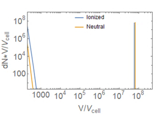
Figure 8: The size distribution of ionized regions and neutral regions at $\bar{x}_{\rm HI}=0.5250$.

Initially, $V_{3}$ has a positive peak around $T_{b}=0$, reflecting the fact that even down to $x_{\rm HI}\sim 0.5$, the ionized regions are still in some sense surrounded by neutral regions. When the neutral fraction drops to around 0.3, however, the $V_{3}$ at $T_{b}=0$ become negative. This is the sign that there are similar number of “holes” (neutral regions inside ionized region) to that of “balls” (ionized regions inside neutral region). We note that there is an asymmetry in the evolution of topology as a function of the global neutral fraction, which may help to explain why the analytical “bubble model” and semi-numerical models based on the same idea works fairly well statistically throughout most of the epoch of reionization.

The other MFs also show interesting evolution during this stage. The volume fraction $V_{0}$ now exhibits a cliff-like initial drop at $T_{b}\sim 0$, then it changes to a shallower decrease. This very steep initial drop does not reach $x_{\rm HI}$ however, but only down some point higher than it. In earlier discussions we noted that the smoothing effect make the drop of $V_{0}$ less steep. The appearance of the very steep initial drop shows that at this stage of reionization, some very large ionized regions are present, so that they are not affected by the smoothing. However, some of the ionized regions are still small which are subject to the smoothing effect, so the $V_{0}$ changes to a more gentle decline before reaching $x_{\rm HI}$. Looking more carefully, there is a small bounce at the bottom of its initial drop. As $V_{0}(x)$ is the fraction of volume with $T_{b}>x$, it should be monotonically decrease. The peak in the surface area $V_{1}$ and the trough in the mean curvature $V_{2}$ at $T_{b}\sim 0$ becomes more prominent, consistent with the impression that the interface between the neutral and ionized regions are highly complicated for the sponge-like topology in this stage.

The fact that the neutral region still surrounds the ionized regions after the Universe is $50\%$ ionized can also be seen using the size distribution of ionized region as shown in Figure 8. Both the largest neutral region and the largest ionized region appear as a dominant cell cluster in this figure, and they have comparable volumes. However, the number of small ionized regions and neutral regions have a significant difference, with many more (two orders of magnitude higher) ionized regions than its neutral counterparts. The bubbles are much more numerous than the islands, hence the positive Euler characteristics.

4.4 The Neutral Fibers Stage

As the redshift decreases further, most of the cosmic volume become occupied by the ionized regions, and we expect to enter a neutral fibers stage, which in some sense can be regarded as the mirror of the ionized fiber state: the neutral regions are now embedded within the ionized regions, but most of the neutral regions are connected.

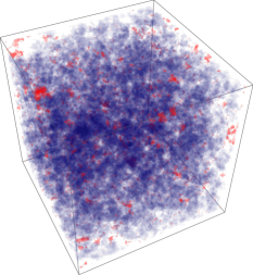
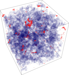
Figure 9: The largest neutral region(blue) and other neutral regions(red) at $z=7.35,x_{\rm HI}=0.2548$ (top) and $z=7.25,x_{\rm HI}=0.1601$. The ionized regions are left transparent.

Two curves in the last column of Fig. 2 are the MF during this stage. The first curve, which is the same as the last curve of the last stage, with $z=7.375,x_{\rm HI}=0.2548$ (red solid line), and the second has $z=7.25,x_{\rm HI}=0.1601$ (blue dash line).

Now the $V_{0}$ has an even larger steep initial drop at $T_{b}=0$, though still not down to $x_{\rm HI}$ during this steep drop due to the smoothing effect. The surface area $V_{1}$ at $T_{b}=0$ decreases a bit as the neutral region begin to shrink. The negative trough of $V_{2}$ also become less deep. The trough of $V_{3}$ deepens however, showing that there are more “tunnels” than the ”holes”, and the neutral region remain to have a highly complicated topology. However, at $x_{\rm HI}=0.16$ the $V_{3}$ drops to a minimum, approaching the percolation threshold.

In Fig. 9 we show the largest neutral region in blue and all other neutral regions in red, while ionized regions are transparent. We can see the largest neutral region has a fiber-like morphology, similar to the ionized regions during the ionized fiber stage. At the lower redshift with $x_{\rm HI}=0.16$, the size of the largest fiber decrease, and some of its branches are cut off by ionization and become small, independent neutral regions.

4.5 The Neutral Islands Stage

As the reionization progress further, the connected network of neutral regions gradually break into pieces and become isolated neutral islands. The last curve in the last column of Fig. 2, $z=7.1,x_{\rm HI}=0.023$ shows this final stage of reionization.

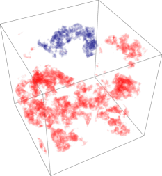
Figure 10: The largest neutral region(blue) with other neutral regions(red) as simulated with 21cmFAST at $z=7.1,x_{\rm HI}=0.023$, ionized cells are left transparent.

The volume fraction $V_{0}$ now drops as a cliff at $T_{b}>0$, to almost zero, then bounces back to a value slightly larger than $x_{\rm HI}$, due to smoothing. For the surface area $V_{1}$, the peak at $T_{b}=0$ lowers as the number and area of the neutral region is decreasing, and at higher $T_{b}$ it almost vanished. The trough at $T_{b}=0$ for the mean curvature $V_{2}$ and the Euler characteristic $V_{3}$ also has the same vanishing trend. Furthermore, during the Neutral Fibers stage there is still some peaks in $T_{b}\gg 0$, indicating the presence of some dense clumps inside the large neutral region, these now also disappeared. At this point, most neutral regions are isolated, contributing the number of “holes”, and the island model description becomes applicable.

After the neutral islands become isolated, they continue to shrink and disappear, resulting the decreasing value of $V_{3}$ around $T_{b}\sim 0$. Eventually, all the islands are ionized and $V_{3}$ returns to 0 as the reionization is completed. In Fig.10 we show the largest neutral region in blue, and other neutral regions in red. Here we see even the largest neutral region is now relatively small, but there are still numerous small islands. However, all of these neutral will be reionized eventually.

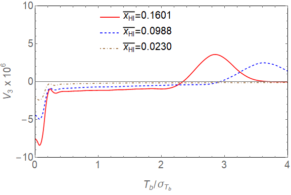
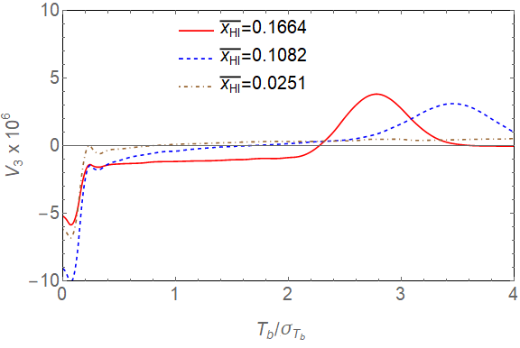
Figure 11: The evolution of $V_{3}$ simulated with 21cmFAST (top panel) and IslandFAST (bottom panel).

5 IslandFAST vs. 21cmFAST

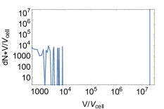
(a) $\bar{x}_{\rm HI}=0.1601$, 21cmFAST

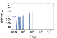
(b) $\bar{x}_{\rm HI}=0.0988$, 21cmFAST

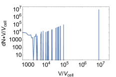
(c) $\bar{x}_{\rm HI}=0.0687$, 21cmFAST

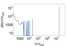
(d) $\bar{x}_{\rm HI}=0.1664$, IslandFAST

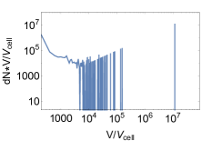
(e) $\bar{x}_{\rm HI}=0.1082$, IslandFAST

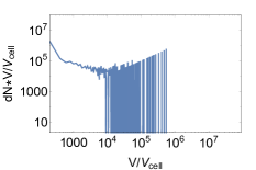
(f) $\bar{x}_{\rm HI}=0.0769$, IslandFAST

Figure 12: Size distribution of neutral regions in each neutral fraction from $x_{\rm HI}\sim 0.17$ to $\bar{x}_{\rm HI}\sim 0.07$. The top panel are results of 21cmFAST, and the bottom panel are results for islandFAST.

In the above, the evolution of the ionization field were obtained by using the 21cmFAST semi-numerical simulation. However, the external photons from the ionizing background may play an important role in the later stages of reionization. This is taken into account by the IslandFAST model. Here we make a re-analysis of the later stages by comparing the results of the 21cmFAST and IslandFAST simulations. The IslandFAST requires an input on the external ionizing background at the start, though afterwards the ionizing background at each later redshift is derived self-consistently. Here we started the IslandFAST simulation at $x_{\rm HI}=0.17$, using the output of the 21cmFAST at that redshift as initial condition. We then compare the subsequent topological evolution for the two models.

The evolution of $V_{3}$ as simulated with IslandFAST and 21cmFAST are shown in Figure 11. As the evolution in the two models are different, we take the results at approximately equal neutral fractions.

For the 21 cm field simulated with 21cmFAST, the $V_{3}$ at $T_{b}=0$ simply increases monotonically during this era, indicating a continuous decrease in the number of individual islands. For the IslandFAST, however, $V_{3}$ at $T_{b}=0$ first decrease to a lower minimum, then begin to increase. The further decrease in $V_{3}$ for the IslandFAST simulation reflects the process that the relatively large neutral regions are being divided into smaller ones because of the bubbles-in-island effect, as well as the increasing ionizing background. This process creates more “holes”, resulting in a more negative $V_{3}$ around $T_{b}=0$. Eventually, the isolated neutral islands are consumed by the ionizing background, and similar to the case with 21cmFAST, the $V_{3}$ at $T_{b}=0$ eventually vanishes.

In Fig. 12 we plot the size distribution function of the two simulations at three comparable neutral fractions (the neutral fractions are derived from the simulation snapshots, so they can not be made exactly equal). The top panels (a,b,c) show the 21cmFAST results, while the bottom panels (d,e,f) show the IslandFAST result. For 21cmFAST, the neutral region simply shrinks as the neutral fraction decreases, so that the whole neutral region size distribution simply shifts toward smaller ones, but a very large neutral cluster is always present. For IslandFAST, however, at certain point the largest neutral region breaks into disconnected pieces around $x_{\rm HI}\sim 0.1$, so the largest island disappears, while the number of smaller ones is nearly constant or even get an increase during this process. This evolution in the number of neutral islands as a function of average neutral fraction is also plotted in Fig. 13. At the starting point $x_{\rm HI}=0.17$, the number of islands in the 21cmFAST simulation and the IslandFAST simulation are the same. As $x_{\rm HI}$ decreases, however, the two models diverge. For 21cmFAST, the number of neutral regions as well as the volume of the largest neutral region decreases monotonically. For IslandFAST, as $x_{\rm HI}$ drops to $\approx 0.1$, the large neutral region breaks into a number of smaller islands, with a sudden increase of the number of neutral regions. Of course, for either code, the number of islands approaches zero with $x_{\rm HI}\to 0$.

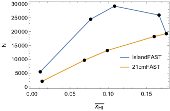
Figure 13: The number of islands as a function of average neutral fraction as simulated with 21cmFAST and IslandFAST.

From these results, we observe that during the late stage of the reionization, the IslandFAST simulation predicts that the largest neutral region gets cut off into multiple pieces, while in the 21cmFAST it shrinks, though at some point it must also be broken off into two or a few pieces, as it no longer percolate through the whole box. This is not surprising, the IslandFAST takes the ionization caused by external photons into account explicitly, such photons are more uniformly distributed, and would more likely to cut through the links between the neutral regions at the same time, and this perhaps provides a better description of the topological evolution during the late stage of EoR.

6 Observablity

We now study the feasibility of using the MFs to distinguish the various stages. The reionization process are very complicated and there are a very wide range of possibilities, it is not possible to cover or even explore all these possibilities here. For example, For example, if the ionizing photon spectrum are produced by quasars or decaying particles and very hard, many regions will be partially ionized and the scenarios would be entirely different. Instead, we will use our fiducial model to illustrate how the MFs can be used as a quantitative tool to distinguish these stages, and similar analysis with the MFs can be performed on models not too different. For simplicity, we select one feature for each stage transition and list them in Table 1, but we do NOT claim that these are universal criteria applicable to all models.

Table 1: A summary of the MF features at transition points

Stage⋆	$\bar{x}^{c}_{\rm HI}$	Feature
1 $\to$ 2	0.9	The fractional difference of the
		two peaks of $V_{3}>0.1$
2 $\to$ 3	0.7	The trough in $V_{2}$ shifts leftwards
		to $T_{b}\approx 0$
3 $\to$ 4	0.3	$V_{3}$ around $T_{b}\sim 0$ becomes negative
4 $\to$ 5	0.1 or 0.16†	The trough in $V_{3}$ reaches its minimum

^⋆ The numbered stages are 1.the Ionized Bubbles stage, 2. the Ionized Fibers stage, 3. the Sponge stage, 4. the Neutral Fibers stage and 5. Neutral Islands stage.
^† The mean neutral fraction at the last transition is about 0.16 in 21cmFAST and about 0.10 in islandFAST.

For the Square Kilometer Array phase one low frequency experiment (SKA1-low), the angular and frequency resolutions are much finer than the comoving smoothing scale (16 Mpc) used for our MF measurement, so instrumental smearing is negligible. We assume the per pixel noise is Gaussian and given by (e.g. Watkinson & Pritchard 2014):

$$\sigma_{\rm{noise}} = 2.9\left(\frac{10^{5}\rm{m^{2}}}{A_{\rm{eff}}}\right)\left(\frac{10^{\prime}}{\Delta\theta}\right)^{2}\left(\frac{1+z}{10.0}\right)^{4.6}$$ (10)

$$\times\sqrt{\frac{1\,\rm{MHz}}{\Delta\nu}\frac{100\,\rm{hours}}{t_{\rm{int}}}}\rm{mK},$$

with the system temperature $T_{\rm sys}\approx T_{\rm sky}$ with (Mozdzen et al., 2015)

$$T_{\rm sky}=180\left(\frac{\nu}{180\,{\rm MHz}}\right)^{-2.6}\rm{K}.$$ (11)

The array sensitivity $A_{\rm{eff}}/T_{\rm{sys}}$ is modeled according to the SKA performance document, and we assume an integration time of 1000 hours. For $z=8.5$ and $\bar{x}_{\rm HI}=0.72$ in our fiducial model, the signal to noise ratio $\approx$10 per smoothing pixel ($(16\,{\rm Mpc})^{3}$).

6.1 The measurement error of MFs

Both the 21cm temperature and the thermal noise on each pixel are random. To estimate the error on MFs, we generate different realizations of the 21cm field as well as the noise, and compute the sample variance.

First we consider the effect of cosmic variance of the 21cm field. We re-simulate the reionization process with 8 independent realizations using the same parameters. The results are shown as the blue shadows (below the y-axis) in Fig. 14. As expected, the MFs in the different realizations are similar and the deviations are small, showing that the MFs are indeed good statistical observables. This is achieved with the 1 Gpc box, which at $z\sim 7$ corresponds to an $6.5^{\circ}\times 6.5^{\circ}$ area. For comparison, a fiducial value of the SKA deep field is about $20\,{\rm deg}^{2}$ (Greig et al., 2019). Note that the error of the MFs approximately scales as $V^{-1/2}$, as we verified using the simulation.

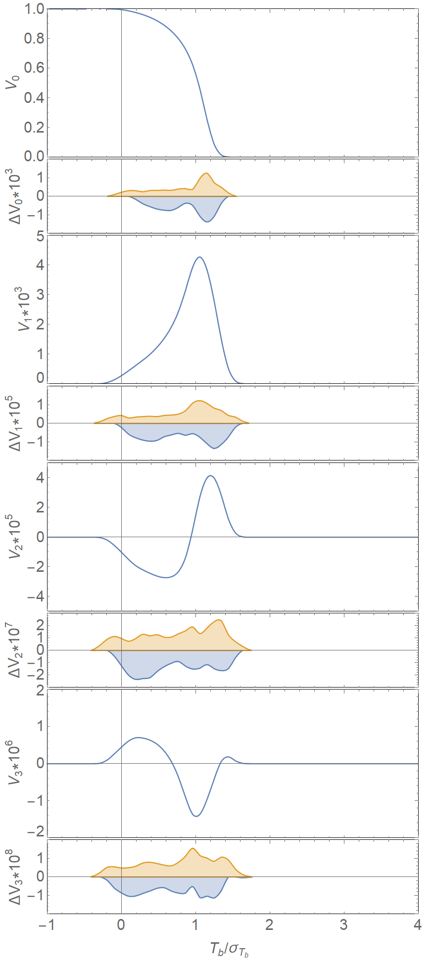
Figure 14: A typical set of MFs with cosmic variance denoted as $\Delta V_{i}$ at $\bar{x}_{HI}\sim 0.72$. The orange shadow (above the y-axis) represents the sampling error from 30 different realizations of thermal noise. The blue shadow (below the y-axis) represents the sampling error derived from the 8 different realizations of simulation.

Second, we generate 30 different realizations of thermal noise, and plot the sample variance with the orange shadow (upper half of the y-axis) in Fig. 14. The variance between them are also quite small. However, the thermal noise has a Gaussian distribution, as a result its impacts on the Minkowski functionals are biased. The observed 21cm field, which is a superposition of the 21cm field and the thermal noise has a more Gaussian distribution than the 21cm field alone. The features in the MFs come mainly from the topology of the $T_{\rm b}=0$ contours which correspond to the boundaries between neutral and ionized regions, i.e. ionizing fronts, such a contour is sensitive to the addition of the thermal noise, as already pointed out in previous works on the bubble and island statistics (Giri et al., 2019, 2018). In Fig. 15, we show the MFs for the no noise case, the small noise case which corresponding to the one simulated above, and the large noise case which is obtained by magnifying the thermal noise by a factor of 3 so that the signal to noise ratio is $\sim$ 3, the results are shown in Fig. 15. The MFs of the small noise case are almost identical to those of the no noise case. However, in the large noise case, the shape of MFs becomes very similar to the MFs of Gaussian random field as illustrated in Fig. 1, effectively wiping out the features of the percolation cluster. The MFs are only effective reionization topology indicators when large signal to noise ratio observation data is available.

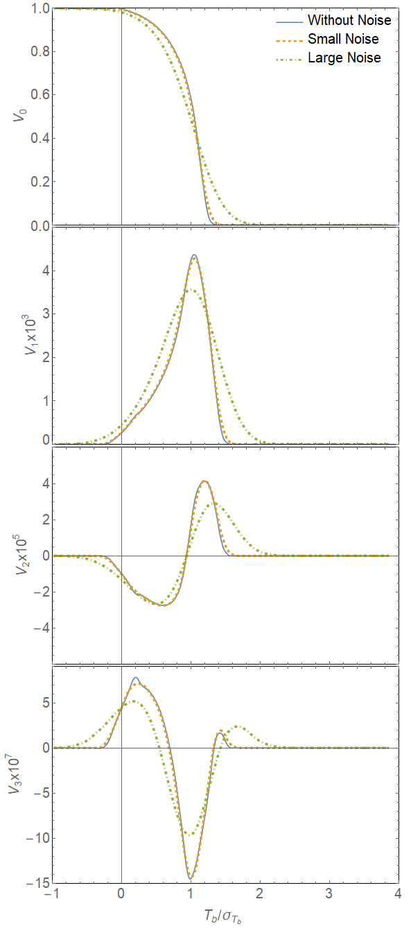
Figure 15: MFs at $\bar{x}_{\rm HI}\sim 0.72$ with no noise, small noise ($\rm SNR\sim 10$) and large noise ($\rm SNR\sim 3$). The $V_{2}$ and $V_{3}$ with noise are multiplied by 10 for better view.

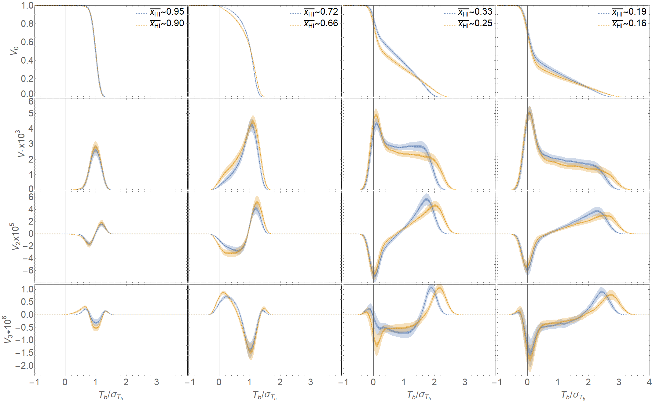
Figure 16: The simulated observation of MFs and errors taken into account of the light cone effect at a few redshifts during EoR. In each column we show the results of two mean neutral fractions which are before (blue) and after (orange) a transition discussed in this paper. For each the lighter shadow shows the error taken with a measurement of $(1\,{\rm Gpc})^{2}\times 48\,{\rm Mpc}$, while the darker shadow shows the error with a measurement of $(5\,{\rm Gpc})^{2}\times 48\,{\rm Mpc}$.

6.2 The light cone effects

In the above we have simulated the measurement of MFs at a given time or redshift in a comoving three dimensional box. However, in real observations one can only make the measurement along the light cone, the near and far sides of the survey volume correspond to different redshifts. The size of the volume in which the measurement is made must then be limited, such that the evolution is not too much during the light travel time across the box. For reionization, this poses a serious problem, because the ionization fraction are changing rapidly. If one take a redshift interval of $\delta z\sim 0.2$ at $z=8.5$, for example, it corresponds to only about $\delta L\sim 50\,\rm{Mpc}$ along the line of sight. As our smoothing length is $R_{\rm{pix}}=16\,\rm{Mpc}$, a “realistic” observation can cover only about three slices. If such small volume is used, the uncertainties would be significant. This light cone effect has been well known in the power spectrum measurement (e.g. Datta et al. 2012, 2014).

Taking boxes of a thickness of $\delta L=48\,{\rm Mpc}$, we calculate the MFs and the expected errors, the results are shown in Fig. 16. Here on each column we plot the results just before(in blue color) or after (in orange color) one of the transition of stages discussed above. The large lighter shadow depicts the expected error for a survey volume of $(1\,{\rm Gpc})^{2}\times 48\,{\rm Mpc}$. Due to the light cone effect, the error is much larger than the previously discussed sampling errors. Nevertheless, in few cases the differences are still large enough to be distinguished easily, but in other cases the differences are just comparable to the measurement errors. However, the measurement error can be reduced by observing a larger sky area. As noted earlier, the error of MFs roughly scales as $V^{-1/2}$. For a fixed redshift interval limited by the light cone effect, the error can be reduced to acceptable level by having a larger sky area. We also show in the darker shadow area in Fig. 16 the result with a survey of $(5\,{\rm Gpc})^{2}\times 48\,{\rm Mpc}$, with the same integration time per pixel. This would require a quite large amount of observing time, but may still be achieved over several years, and the process can be speed up if the SKA-low is equipped with multi-beam forming capability.

7 Discussions

We have analyzed the evolution of the topological structure of the 21 cm brightness temperature field during EoR using a set of semi-numerical simulations. The ionized regions have a brightness temperature of $T_{b}=0$, while the neutral regions have $T_{b}>0$. By tracking the changes of MFs, especially by looking at the MFs at just above $T_{b}=0$, one can gain insights on the topology of the ionization-neutral region interface during the reionization process.

Based on the analysis of the MFs and other statistics, e.g. the size distribution of the neutral and ionized regions, we find that the topological evolution of the reionization process can be divided into five different stages. In the first stage where the neutral fraction $x_{\rm HI}\gtrsim 0.9$, there are numerous isolated ionized regions (“bubbles”). As more numerous and larger bubbles formed, the ionized regions begin to connect with each other. Next, the ionized regions formed cluster structures (“ionized fibers”), with the largest one percolating through the whole simulation box. At $x_{\rm HI}\approx 0.7$, most of the ionized regions overlap with each other, forming a connected structure intertwined with a similar structure of neutral regions, the whole space of ionized and neutral regions takes the appearance of a “sponge”. As the reionization progress further, the neutral regions begin to shrink and being surrounded by the ionized regions, at $x_{\rm HI}\lesssim 0.3$, a “neutral fiber” stage set in. Finally, the neutral fiber also shrinks and at some point around $x_{\rm HI}\sim 0.16$ it no longer percolate through the whole simulation box, and we enter the stage of isolated “neutral islands”.

From the results summarized above, we see that strictly speaking, the original assumptions of the bubble model and island model, namely that the ionized regions or the neutral regions are isolated, are only valid during the first or the last stage of the reionization process. During the intermediate stages, the topology of the region could be fairly complicated, and as a result the numerical model may not be quantitatively accurate, as have been noted in previous works (Xu et al., 2014; Furlanetto et al., 2006). Nevertheless, it is interesting to note that the semi-numerical simulations which are based on spherical averages do produce very complex and irregular shaped regions. The bubble model and island model are based on the balance between the number of photons needed for ionization and the number of photons produced locally (bubble model) and also the number of photons from the external background (for the island model). The fiber-like shape in such models originates from the shape of the iso-density contours of the density fluctuations. Very recently, Bag et al. (2018) used the MFs and cluster statistics to characterize the topology of the ionized regions, they also found the fiber-like shapes of the ionized regions, and using the shapefinder statistics derived from the MFs, they found that the cross-section of the fibers are nearly constant. The numerical algorithm we adopted is not suitable for accurate computing of the shapefinder statistics, but this result is consistent with the general picture of reionization process we delineated above.

Compared with the original assumption, the most important difference for the fiber shaped ionized region is that they will get some additional ionizing photons from the connected neighboring cells, i.e. some ionizing photons can propagate along the fibers, so that the ionization may be even faster. However, if the ionized regions are indeed shaped as fibers, the cross section for the background photon is fairly limited, and the zigzag path also limit the distance the photons could travel due to finite propagation time and the absorption by the residue neutral gas in the ionized regions. Thus, even though the original assumption of isolated bubbles is no longer true during the ionized fiber stage, we speculate that the model may still give reasonably good predictions. For the neutral fibers, the inaccuracy of the 21cmFAST model may be larger, as a substantial amount of the photons could come from the surrounding ionizing background. However, the IslandFAST program may take into account of the surface area of the actual neutral region, the main difference in topology is that the neutral fibers are more prone to break-up into smaller islands.

We found that although the value of MFs are affected by thermal noise, which is more Gaussian than the signal and thus making the MFs more bland, there remains features which can be used to distinguish the different stages, at least with high signal-to-noise measurements (${\rm SNR}\sim 10)$). However, due to the rapid evolution of the ionization fraction during EoR, the light cone effect put a limit on the usable redshift bin size ($\Delta z\lesssim 0.2$). For a typical SKA EoR survey with an area of $\sim 40\,{\rm deg}^{2}$ and 1000 hour integration time per pixel, in some cases the MFs can still be distinguished though for many cases the difference would be comparable to the measurement errors. To achieve a good measurement, a larger sky area is needed. Thus, the evolution of topology is within the reach through 21 cm brightness temperature measurements using SKA-low, though it may require a survey of many years to complete. The survey time could be shortened if the SKA-low is equipped with multi-beam forming capability.

The present study is still limited in several ways. Our study is based on semi-numerical models, which is only an approximation and can not replace a full radiative transfer simulation. The study of the topology of reionization using the semi-numerical models may be considered as a self-consistent check on the basic assumptions of the method. We have limited our presentation to the results obtained for a fiducial model. The different cosmological and reionization parameters may affect the results. However, from a few exploratory tests, it seems that as long as the ionizing sources are soft ones which produce clear boundary between the neutral and ionized regions, and the cosmological parameters and reionization parameters are not too extreme, the general picture of the evolution presented above should be robust.

References

- Akrami et al. (2018) Akrami, Y., et al. 2018, 1807.06205
- Bag et al. (2019) Bag, S., Mondal, R., Sarkar, P., Bharadwaj, S., Choudhury, T. R., & Sahni, V. 2019, MNRAS, 485, 2235
- Bag et al. (2018) Bag, S., Mondal, R., Sarkar, P., Bharadwaj, S., & Sahni, V. 2018, Mon. Not. Roy. Astron. Soc., 477, 1984
- Bond et al. (1991) Bond, J. R., Cole, S., Efstathiou, G., & Kaiser, N. 1991, Astrophys. J., 379, 440
- Bowman et al. (2018) Bowman, J. D., Rogers, A. E. E., Monsalve, R. A., Mozdzen, T. J., & Mahesh, N. 2018, Nature, 555, 67
- Chen & Miralda-Escude (2004) Chen, X.-L., & Miralda-Escude, J. 2004, Astrophys. J., 602, 1
- Datta et al. (2014) Datta, K. K., Jensen, H., Majumdar, S., Mellema, G., Iliev, I. T., Mao, Y., Shapiro, P. R., & Ahn, K. 2014, Mon. Not. Roy. Astron. Soc., 442, 1491
- Datta et al. (2012) Datta, K. K., Mellema, G., Mao, Y., Iliev, I. T., Shapiro, P. R., & Ahn, K. 2012, Mon. Not. Roy. Astron. Soc., 424, 1877
- Dayal & Ferrara (2018) Dayal, P., & Ferrara, A. 2018, Phys. Rep., 780, 1
- DeBoer et al. (2017) DeBoer, D. R., et al. 2017, Publ. Astron. Soc. Pac., 129, 045001
- Fan et al. (2006) Fan, X.-H., Carilli, C. L., & Keating, B. G. 2006, Ann. Rev. Astron. Astrophys., 44, 415
- Furlanetto et al. (2006) Furlanetto, S., Oh, S. P., & Briggs, F. 2006, Phys. Rept., 433, 181
- Furlanetto et al. (2004) Furlanetto, S., Zaldarriaga, M., & Hernquist, L. 2004, Astrophys. J., 613, 1
- Furlanetto & Oh (2016) Furlanetto, S. R., & Oh, S. P. 2016, Mon. Not. Roy. Astron. Soc., 457, 1813
- Giri et al. (2019) Giri, S. K., Mellema, G., Aldheimer, T., Dixon, K. L., & Iliev, I. T. 2019, 1903.01294
- Giri et al. (2018) Giri, S. K., Mellema, G., Dixon, K. L., & Iliev, I. T. 2018, Mon. Not. Roy. Astron. Soc., 473, 2949
- Gleser et al. (2006) Gleser, L., Nusser, A., Ciardi, B., & Desjacques, V. 2006, Mon. Not. Roy. Astron. Soc., 370, 1329
- Greig et al. (2019) Greig, B., Mesinger, A., & Koopmans, L. V. E. 2019, 1906.07910
- Hong et al. (2014) Hong, S. E., Ahn, K., Park, C., Kim, J., Iliev, I. T., & Mellema, G. 2014, Journal of Korean Astronomical Society, 47, 49
- Kapahtia et al. (2018) Kapahtia, A., Chingangbam, P., Appleby, S., & Park, C. 2018, Journal of Cosmology and Astro-Particle Physics, 2018, 011
- Kittiwisit et al. (2018) Kittiwisit, P., Bowman, J. D., Jacobs, D. C., Beardsley, A. P., & Thyagarajan, N. 2018, Mon. Not. Roy. Astron. Soc., 474, 4487
- Koenderink (1984) Koenderink, J. J. 1984, Biological Cybernetics, 50, 363
- Lacey & Cole (1993) Lacey, C. G., & Cole, S. 1993, Mon. Not. Roy. Astron. Soc., 262, 627
- Lee et al. (2008) Lee, K.-G., Cen, R., Gott, III, J. R., & Trac, H. 2008, ApJ, 675, 8
- Maartens et al. (2015) Maartens, R., Abdalla, F. B., Jarvis, M., & Santos, M. G. 2015, PoS, AASKA14, 016
- Mesinger et al. (2011) Mesinger, A., Furlanetto, S., & Cen, R. 2011, Mon. Not. Roy. Astron. Soc., 411, 955
- Minkowski (1903) Minkowski, H. 1903, Mathematische Annalen, 57, 447
- Mozdzen et al. (2015) Mozdzen, T. J., Bowman, J. D., Monsalve, R. A., & Rogers, A. E. E. 2015, Monthly Notices of the Royal Astronomical Society, 455, 3890
- Paciga et al. (2011) Paciga, G. et al. 2011, Mon. Not. Roy. Astron. Soc., 413, 1174
- Parsons et al. (2010) Parsons, A. R., et al. 2010, Astron. J., 139, 1468
- Saberi (2015) Saberi, A. A. 2015, Phys. Rep., 578, 1
- Schmalzing & Buchert (1997) Schmalzing, J., & Buchert, T. 1997, ApJ, 482, L1
- Shimabukuro et al. (2016) Shimabukuro, H., Yoshiura, S., Takahashi, K., Yokoyama, S., & Ichiki, K. 2016, Mon. Not. Roy. Astron. Soc., 458, 3003
- Songaila & Cowie (2010) Songaila, A., & Cowie, L. L. 2010, ApJ, 721, 1448
- Tingay et al. (2013) Tingay, S. J., et al. 2013, Astron. J., 146, 103
- van Haarlem et al. (2013) van Haarlem, M. P., et al. 2013, Astron. Astrophys., 556, A2
- Wang et al. (2015) Wang, Y., Park, C., Xu, Y., Chen, X., & Kim, J. 2015, Astrophys. J., 814, 6
- Watkinson & Pritchard (2014) Watkinson, C. A., & Pritchard, J. R. 2014, Mon. Not. Roy. Astron. Soc., 443, 3090
- Wyithe & Morales (2007) Wyithe, S., & Morales, M. F. 2007, Mon. Not. Roy. Astron. Soc., 379, 1647
- Xu et al. (2017) Xu, Y., Yue, B., & Chen, X. 2017, Astrophys. J., 844, 117
- Xu et al. (2014) Xu, Y., Yue, B., Su, M., Fan, Z., & Chen, X. 2014, Astrophys. J., 781, 97
- Yoshiura et al. (2017) Yoshiura, S., Shimabukuro, H., Takahashi, K., & Matsubara, T. 2017, Mon. Not. Roy. Astron. Soc., 465, 394
- Zahn et al. (2006) Zahn, O., Lidz, A., McQuinn, M., Dutta, S., Hernquist, L., Zaldarriaga, M., & Furlanetto, S. R. 2006, Astrophys. J., 654, 12
- Zentner (2007) Zentner, A. R. 2007, Int. J. Mod. Phys., D16, 763