Gravity-Mediated SUSY Breaking,
$R$ Symmetry and Hyperbolic Kähler Geometry

Abstract

Abstract: A novel realization of the gravity-mediated SUSY breaking is presented taking into account a continuous global $R$ symmetry. Consistently with it, we employ a linear superpotential for the hidden sector superfield and a Kähler potential parameterizing the $SU(1,1)/U(1)$ Kähler manifold with constant curvature $-1/2$. The classical vacuum energy vanishes without unnatural fine tuning and non-vanishing soft SUSY-breaking parameters, of the order of the gravitino mass, arise. A solution to the $\mu$ problem of MSSM may be also achieved by conveniently applying the Giudice-Masiero mechanism. The potentially troublesome $R$ axion may acquire acceptably large mass by explicitly breaking the $R$ symmetry in the Kähler potential through a quartic term which does not affect, though, the achievements above.

PACs numbers: 12.60.Jv, 04.65.+e Published in Phys. Rev. D 100, no. 5, 055013 (2019)

I Introduction

Although still undiscovered, Supersymmetry (SUSY) remains one of the most plausible, well-motivated and natural candidates for the evolution of particle physics beyond the Standard Model (SM). One of the most elusive problems of the SUSY theories is the mechanism of the SUSY breaking. According to an elegant and extensively adopted paradigm, SUSY is spontaneously broken by the vacuum expectation values (v.e.vs) of a set of chiral fields which form a “hidden sector” nilles connecting with the observable sector mostly through gravitational-strength interactions, including the effects of Supergravity (SUGRA).

One of the key ingredients for the successful implementation of this scenario is the determination of a realistic vacuum for the relevant SUGRA potential with naturally vanishing or, at least, tunably small cosmological constant. In view of the recent scepticism vafa ; lindev related to the consistency of the de Sitter vacua within string theory, we here concentrate on the former possibility proposing a novel gravity-mediated SUSY-breaking scenario with natural Minkowski solutions at the classical level. Actually, we improve the well-known Polonyi model polonyi in two directions: Following Ref. hall , we keep only the first term of the relevant superpotential which includes a linear term of the hidden sector field and may become consistent with a global $R$ symmetry rnelson forbidding other terms. The vanishing of cosmological constant is elegantly addressed by selecting an appropriate internal space which exhibits a $SU(1,1)/U(1)$ symmetry linde1 ; linde ; su11 with constant curvature $-1/2$. Using a convenient parametrization of the Kähler manifold, which violates though the $R$ symmetry, we show that our model exhibits novel Minkowski solutions in the context of the generalized no-scale SUGRA noscale ; noscale1 ; noscale18 . Contrary to that case noscale13 , the gravitino, $\widetilde{G}$, mass is clearly determined at the tree level and the soft SUSY-breaking (SSB) parameters soft can readily acquire adjustable, non-zero values of the order of $\widetilde{G}$ mass. We exemplify these effects, linking the hidden sector to a generic SUSY model and the Minimal Supersymmetric SM (MSSM). In the latter case, our scheme also offers an explanation of the $\mu$ term of MSSM by conveniently adapting the Giudice-Masiero mechanism masiero .

However, a spontaneously broken continuous and global $R$ symmetry implies an (pseudo) Nambu-Goldstone boson, the $R$ axion, rnelson ; raxion – as in the case of Peccei-Quinn symmetry pq – which is cosmologically dangerous. To avoid this effect, we introduce a quartic term, inspired by Ref. noscale18 , in the Kähler potential which violates $R$ symmetry and allows for non-vanishing $R$-axion masses without disturbing, though, either the minimization of the SUGRA potential or the values of the SSB parameters.

Below, in Sec. II, we outline the SUGRA formalism and then we focus first, in Sec. III, on the hidden sector and then, in Sec. IV, on the visible sector of our model. Our conclusions and several perspectives are discussed in Sec. V. Possible connection of our model with no-scale SUGRA is examined in Appendix A. Unless otherwise stated, we use units where the reduced Planck mass $m_{\rm P}=2.433\cdot 10^{18}~{}{\mbox{\rm GeV}}$ is taken to be unity and charge conjugation is denoted by a bar.

II SUGRA Formalism

In constructing a SUSY-breaking model based on SUGRA, we mostly consider two sectors; a so-called hidden sector responsible for the spontaneous SUSY breaking, and an observable sector which includes ordinary matter and Higgs fields and which would have unbroken global SUSY in the absence of the coupling to SUGRA. In particular, it is assumed that the superpotential has the form

$$W=W_{\rm H}(Z)+W_{\rm O}\left(\Phi_{\alpha}\right),$$ (1)

in which $W_{\rm H}$ and $W_{\rm O}$ depend only on the chiral fields of the hidden and observable sectors, respectively. The hidden sector here consists of just one gauge-singlet superfield $Z$, similarly to the Polonyi polonyi model, whereas the superfields of the observable sector are denoted by $\Phi_{\alpha}$. The suggested Kähler potential may take collectively the form

$$K=K_{\rm H}(Z)+\widetilde{K}(Z)|\Phi_{\alpha}|^{2}.$$ (2)

The specific expressions for $W_{\rm H}$ and $K_{\rm H}$ are given in Sec. III whereas those for $W_{\rm O}$ and $\widetilde{K}$ in Sec. IV.

Central role in the SUGRA formalism plays the Kähler-invariant function expressed in terms of $K$ and $W$ as follows

$$G=K+\ln|W|^{2}.$$ (3)

Using it we can derive the SUGRA scalar potential

$$V=e^{G}\left(G^{{A}{\bar{B}}}G_{A}G_{\bar{B}}-3\right)=\left(G_{{A}{\bar{B}}}F^{A}\bar{F}^{\bar{B}}-3e^{G}\right),$$ (4)

where the subscripts denote differentiation with respect to (w.r.t) the fields $Z$ and $\Phi^{\alpha}$ and $G^{{A}{\bar{B}}}=K^{{A}{\bar{B}}}$ is the inverse of the Kähler  metric $K_{{A}{\bar{B}}}$. The F terms are defined as soft

$$F^{A}=e^{G/2}K^{{A}{\bar{B}}}G_{\bar{B}}~{}~{}~{}\mbox{and}~{}~{}~{}\bar{F}^{\bar{A}}=e^{G/2}K^{{\bar{A}}{B}}G_{B}\,.$$ (5)

The spontaneous SUSY breaking is signaled by the absorption of a massless fermion named goldstino by $\widetilde{G}$, according to the “super-Higgs” mechanism, and is accompanied by a non-vanishing $\widetilde{G}$ mass evaluated at the minimum of $V$ as follows

$$m_{3/2}=\left\langle{e^{G/2}}\right\rangle=\frac{1}{3}\left\langle{G_{Z{\bar{Z}}}F^{Z}\bar{F}^{\bar{Z}}-V}\right\rangle,$$ (6)

where we made use of Eq. (4) and assume that $\langle{\Phi_{\alpha}}\rangle\ll\left\langle{Z}\right\rangle$. The present vacuum energy density corresponds to $\left\langle{V}\right\rangle\simeq 10^{-120}$, a negligible value w.r.t the SUSY-breaking mass scale $m_{3/2}>10^{-15}$ which implies $\langle{F^{Z}\bar{F}^{\bar{Z}}}\rangle>10^{-30}$. The extraordinarily precise cancellation required in Eq. (4) for fulfilling simultaneously the two above constraints is the notorious cosmological constant problem. Since the explanation of the smallness of $\left\langle{V}\right\rangle$ is the crucial point of this problem and the compatibility of the de Sitter solutions with the string theory is currently under debate vafa ; lindev , we below focus on $\left\langle{V}\right\rangle=0$ which defines a Minkowski vacuum.

Under the assumption above, the mass-squared matrices $M_{J}^{2}$ of the particles with spin $J$ composing the final spectrum of the hidden sector obey the super-trace formula nilles

$${\sf STr}M^{2} = \sum_{J=0}^{3/2}(-1)^{2J}(2J+1)\mbox{\sf Tr}M_{J}^{2}$$ (7)

$$= 2m_{3/2}^{2}\langle{G_{Z{\bar{Z}}}^{-2}G_{Z}G_{{\bar{Z}}}R_{Z{\bar{Z}}}}\rangle,$$

where we take into account that $K_{\rm H}=K_{\rm H}(Z)$. Also, we define the Ricci curvature noscale1 ; linde1 of the Kähler manifold as

$$R_{Z{\bar{Z}}}=-\partial_{Z}\partial_{\bar{Z}}\ln{\rm g}~{}~{}~{}\mbox{with}~{}~{}~{}{\rm g}=\partial_{Z}\partial_{\bar{Z}}K_{\rm H}$$ (8)

being the Kähler  metric of the hidden space, whose the scalar curvature is evaluated from the formula su11

$${\mathcal{R}}_{\rm H}=G^{Z{\bar{Z}}}R_{Z{\bar{Z}}}=\left({\partial_{Z}{\rm g}\partial_{{\bar{Z}}}{\rm g}-{\rm g}\partial_{Z}\partial_{\bar{Z}}{\rm g}}\right)/{{\rm g}^{3}}.$$ (9)

Taking advantage of Eqs. (9) and (4) with $A=Z$ we easily infer that Eq. (7) is translated into

$${\sf STr}M^{2}=6m_{3/2}^{2}\left\langle{{\mathcal{R}}_{\rm H}}\right\rangle,$$ (10)

which is significantly simplified w.r.t the initial one. E.g., in the case of the Polonyi model polonyi with canonical Kähler potential  we obtain ${\rm g}=1$ and so ${\sf STr}M^{2}=0$ nilles .

III Hidden Sector

In this Section we first – see Sec. A – specify the hidden sector of our model and then – see Sec. B – investigate the SUSY-breaking mechanism conserving $R$ symmetry and employing the curvature of the Kähler manifold as free parameter. Perturbing mildly the resulting geometry, we repeat the study, in Sec. C, considering a convenient $R$-symmetry violating term in the Kähler potential.

A Model Set-up

Taking into account the deep conceptual connection rnelson between $R$ symmetry and SUSY-breaking, we fix hall the form of $W_{\rm H}$ in Eq. (1) by imposing an $R$ symmetry under which $Z$ has the $R$ character of $W_{\rm H}$. Namely, we select

$$W_{\rm H}=mZ,$$ (11)

where $m$ is a positive, free parameter with mass dimensions. Contrary to the Polonyi model polonyi and its variants olivegr ; muray , we do not consider any $R$-symmetry violating constant term.

On the other hand, the form of $K_{\rm H}$ in Eq. (2) adopted here may not be totally $R$ invariant. In particular, we set

$$K_{\rm H}=-N\ln\left(1-\frac{|Z|^{2}-kZ_{-}^{n}}{N}\right)~{}~{}\mbox{with}~{}~{}~{}Z_{-}=Z-{\bar{Z}}$$ (12)

and $|Z|<\sqrt{N}$. Here $N,k$ and $n$ are positive free parameters. Motivated by several superstring and D-brane models Ibanez we consider the integer values of $N$ as the most natural. We restrict also ourselves to integer $n$’s. In contrast to the original Polonyi model polonyi and its descendents hall ; olivegr , where flat internal spaces are assumed, $K_{\rm H}$ parameterizes a curved space, with metric

$${\rm g}=Nw\left(N-|Z|^{2}+kZ_{-}^{n}\right)^{-2}$$ (13a)

where

$$w=N-nk^{2}Z_{-}^{2(n-1)}-k(n-1)Z_{-}^{n-2}\left(Z_{-}^{2}+n(|Z|^{2}-N)\right)$$ (13b)

and $n>2$. The $R$-symmetry violation is expressed via $k$ which is a tiny parameter employed to endow $R$ axion – see Sec. C – with mass. Small $k$ values are totally natural, in the ’t Hooft’s sense symm , since nullifying this parameter the $R$ symmetry becomes exact. In the same limit, the Kähler manifold is totally $SU(1,1)/U(1)$ symmetric linde ; noscale1 ; su11 but the Kähler-invariant function – see Eq. (3) – still violates it, due to the form of $W_{\rm H}$ in Eq. (11).

B Totally $R$-Symmetric Case

If we set $k=0$ in Eq. (12) we obtain the exactly $R$-symmetric version of our model which exhibits an hyperbolic space, in Poincaré disk coordinates linde ; su11 , with metric

$${\rm g}^{(0)}=\partial_{Z}\partial_{\bar{Z}}K_{\rm H0}=\left(1-{|Z|^{2}}/{N}\right)^{-2}$$ (14)

and constant curvature estimated by Eq. (9) with result

$${\cal R}_{\rm H}^{(0)}=-2/N~{}~{}~{}\mbox{since}~{}~{}~{}R^{(0)}_{Z{\bar{Z}}}=-{2}{\rm g}^{(0)}/N\,.$$ (15)

Here and hereafter, the superscript $(0)$ and the subscript $0$ denote quantities corresponding to the totally $R$-symmetric case. The same geometry can be expressed in the half-plane coordinates as detailed in Appendix A.

The corresponding SUGRA potential, $V_{\rm H0}$, derived by applying Eq. (4), depends exclusively on $|Z|^{2}$. Indeed, we obtain

$$V_{\rm H0}=\left(\frac{m}{N}\right)^{2}e^{K_{\rm H0}}\left(\left(N+\left(N-1\right)|Z|^{2}\right)^{2}-3N^{2}|Z|^{2}\right),$$ (16)

where we take into account Eq. (14) and the equality

$$G^{(0)}_{Z}=\left(\sqrt{{\rm g}^{(0)}}|Z|^{2}+1\right)/Z=\bar{G}^{(0)}_{\bar{Z}}\,.$$ (17)

We seek below the (preferably integer) value of $N$ that yields a Minkowski vacuum defined by the conditions

$$\mbox{\sf\footnotesize(a)}~{}~{}\left\langle{V_{\rm H0}}\right\rangle=0,~{}~{}\mbox{\sf\footnotesize(b)}~{}~{}\left\langle{V_{\rm H0}^{\prime}}\right\rangle=0~{}~{}~{}\mbox{and}~{}~{}~{}\mbox{\sf\footnotesize(c)}~{}~{}\left\langle{V_{\rm H0}^{\prime\prime}}\right\rangle>0,$$ (18)

where the derivatives w.r.t $|Z|^{2}$ are denoted by a prime. Computing the first derivative of $V_{\rm H0}$ in Eq. (16) w.r.t $|Z|^{2}$, we find

$$V_{\rm H0}^{\prime}=m^{2}\frac{N+(N-1)|Z|^{2}}{e^{1-K_{\rm H0}}N^{3}}\Big{(}(N-1)(N-2)|Z|^{2}-2N\Big{)}.$$ (19)

Taking into account that $|Z|^{2}>0$, we infer that Eq. (18b) implies (for $N\neq 1$ and $N\neq 2$)

$$\left\langle{V_{\rm H0}^{\prime}}\right\rangle=0~{}\Rightarrow~{}\left\langle{|Z|^{2}}\right\rangle=\frac{2N}{(N-2)(N-1)},$$ (20)

which fulfils Eq. (18b) since

$$\left\langle{V_{\rm H0}^{\prime\prime}}\right\rangle=m^{2}\left(\frac{N-2}{N-3}\right)^{N+1}\left(1-\frac{1}{N}\right)^{N+2}>0$$ (21)

for $N>3$. The value of $V_{\rm H0}$ at the minimum is

$$\left\langle{V_{\rm H0}}\right\rangle=m^{2}\frac{N-4}{N-2}\left(\frac{(N-2)(N-1)}{(N-3)N}\right)^{N-1}$$ (22)

and can become consistent with Eq. (18a) for $N=4$. In other words, the value $N=4$ renders the expression in the parenthesis of Eq. (16) equal to the expansion of a perfect square – see Eq. (30) below. In view of Eq. (15), we deduce that the emergence of the Minkowski vacuum is closely connected with the curvature of the internal space which is confined to $R^{(0)}_{\rm H}=-1/2$. The structure of $V_{\rm H0}$ in Eq. (16) is further highlighted in Fig. 1, where we depict it for $N=3,4$ and $5$ (dot-dashed, solid and dashed line respectively) versus $|Z|^{2}$. We observe that for

$$N=4~{}~{}~{}\mbox{and}~{}~{}~{}\left\langle{|Z|^{2}}\right\rangle=4/3$$ (23)

$V_{\rm H0}$ exhibits an absolute minimum with vanishing $\langle{V_{\rm H0}}\rangle$. It is impressive that this goal is attained without any tuning. Obviously, tiny, non-zero $\langle{V_{\rm H0}}\rangle$ can be also achieved by tuning $N$ to values a little larger than $4$.

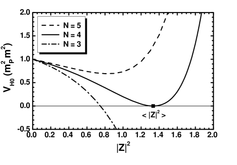
Fig. 1: The (dimensionless) hidden-sector potential $V_{\rm H0}/m^{2}m_{\rm P}^{2}$ in Eq. (16) as a function of $|Z|^{2}$ for $N=3$ (dot-dashed line), $N=4$ (solid line) and $N=5$ (dashed line). The line $V_{\rm H0}=0$ and the value $\left\langle{|Z|^{2}}\right\rangle$ are also indicated.

If we analyze $Z$ according to the description

$$Z=(z+i{\theta})/\sqrt{2}$$ (24)

and expand $V_{\rm H0}$ in Eq. (16) about the configuration

$$\left\langle{z}\right\rangle=2\sqrt{\frac{2}{3}}~{}~{}~{}\mbox{and}~{}~{}\left\langle{{\theta}}\right\rangle=0,$$ (25)

– cf. Eq. (23) –, we obtain the hidden-sector spectrum of the model. This is composed of a massless Nambu-Goldstone boson, ${\theta}$, – referred rnelson to as an $R$ axion –, a massive real scalar field, $\widehat{z}$, called $R$ saxion, with mass $\widehat{m}_{z}$ and the gravitino $\widetilde{G}$ – which absorbs the fermionic partner of the $R$ saxion, the $R$ axino – with mass $m_{3/2}$. The former can be found by substituting Eq. (21) with $N=4$ in the formula

$$\widehat{m}_{z}=\left\langle{\partial^{2}_{\widehat{z}}V_{\rm H0}}\right\rangle^{1/2}=\left\langle{\frac{2V_{\rm H0}^{\prime\prime}|Z|^{2}}{{\rm g}}}\right\rangle^{1/2}=\frac{3\sqrt{3}}{2}m,$$ (26a)

where we take into account that $$\widehat{z}=\sqrt{{\rm g}^{0}}z \langle{\sqrt{{\rm g}^{0}}}\rangle=\langle{\sqrt{{\rm g}}}\rangle=3/2 R \widetilde{G}$$ with – since along the direction in Eq. (25) the -violating term in Eq. (12) vanishes, we do not apply the distinction mentioned below Eq. (15). As regards the mass, Eq. (6) yields

$$m_{3/2}=m\left\langle{e^{K_{\rm H}/2}Z}\right\rangle=\frac{3\sqrt{3}}{2}m\,.$$ (26b)

The masses above satisfy Eq. (10) in view of Eqs. (15) and (23), since

$${\sf STr}M_{0}^{2}=\widehat{m}_{z}^{2}-4m_{3/2}^{2}=-3m_{3/2}^{2}\,.$$ (27)

We see that the mass scale $m$ involved in Eq. (11) is related to $\widetilde{G}$ mass. Its value is not constrained within our scheme. It may lie in the range from TeV until $m_{\rm P}$ with the former choice being favored by the resolution of the gauge hierarchy problem and the latter option being more natural from the point of view of model building.

Since the $R$ symmetry is explicitly broken by the SSB terms only in the observable sector, the $R$ axion remains completely massless if the $R$ symmetry is color, i.e. $SU(3)_{\rm c}$, non-anomalous. To assess the color anomaly we have to know the complete structure of theory, i.e., the $R$ charges of the $SU(3)_{\rm c}$ non-singlet fermions – cf. Refs. univ ; dvali . There are model-dependent mechanisms gaugedR which may render the $R$ symmetry anomalous free. In a such case, the promotion of the global $R$ symmetry to a gauged one surpasses the difficulty with the massless mode since the $R$ axion is absorbed by the corresponding gauge boson via the Higgs mechanism. If the $R$ symmetry is color anomalous, non-perturbative QCD instanton effects anomalies result in a mass for the $R$ axion. Since $\left\langle{z}\right\rangle\sim m_{\rm P}$, the decay constant of the $R$-axion, $f_{R}$, is expected to be of order $m_{\rm P}$ in contradiction with the constraint $10^{-8}\lesssim f_{R}/m_{\rm P}\lesssim 10^{-6}$ implied by the stellar evolution and the dark matter abundance in the universe. The constraint on $f_{R}$ may be fulfilled, though, considering lower fundamental scale in the Kähler potential – cf. Ref. ribe .

In both cases above, another solution to the problem with the massless $R$ axion is the consideration of $Z$ as a nilpotent superfield nilpotent . In such a case, no sgoldstino multiplet appears at the SUSY-breaking vacuum and so no $R$ axion too. Finally, the simplest solution, adopted here, is the explicit breaking of $R$ symmetry via subdominant terms in $W_{\rm H}$ and/or $K_{\rm H}$ which generates a large enough mass for the $R$ axion. In particular, its mass must exceed $10~{}{\rm MeV}$ to evade astrophysical constraints from production in a supernova astro .

C Including the $R$-Symmetry-Breaking Term

Taking advantage of the nice behavior of $V_{\rm H0}$ in Sec. B we fix $N=4$ and we allow for non-vanishing $k$ and integer $n$ values in Eq. (12). Although no purely theoretical motivation exists for this term, we can show that $n$ can be uniquely determined if we require that the resulting SUGRA potential $V_{\rm H}$ takes, along the real direction ${\theta}=0$, the form of $V_{\rm H0}$ in Eq. (16) and the $R$ axion becomes massive.

Initially, it is easy to convince ourselves that g in Eq. (13a) declines from g⁽⁰⁾ in Eq. (14) for $Z={\bar{Z}}$ and $n=1$ or $2$. Therefore, we restrict our analysis to $n\geq 3$. Applying Eq. (4), we find that $V_{\rm H}$ takes the form

$$V_{\rm H}=\frac{m^{2}}{4}e^{K_{\rm H}}\Big{(}\frac{uv}{w}-12|Z|^{2}\Big{)},$$ (28)

where we introduce the quantities

$$u =4+3|Z|^{2}-kZ_{-}^{n-1}\left((4n-1)Z+{\bar{Z}}\right)$$ (29a)

$$v =4+3|Z|^{2}+kZ_{-}^{n-1}\left(Z+(4n-1){\bar{Z}}\right)$$ (29b)

with $u$ and $v$ originating from the numerators of $G_{Z}$ and $G_{\bar{Z}}$ whereas $w$ is given by Eq. (13b) for $N=4$. Using the parametrization in Eq. (24), we can express $V_{\rm H}$ as a function of $z$ and ${\theta}$ and minimize it in both directions to determine the Minkowski vacuum. We can show, though, that the direction ${\theta}=0$ is stable, for $n>3$, and so the Minkowski vacuum still lies along the direction in Eq. (25).

Indeed, $V_{\rm H}$ for ${\theta}=0$ coincides with the one obtained from Eq. (16) for $N=4$, i.e.,

$$V_{\rm H}(z,{\theta}=0)=64m^{2}\frac{(3z^{2}-8)^{2}}{(z^{2}-8)^{4}}$$ (30)

and therefore, $\left\langle{z}\right\rangle$ keeps its value in Eq. (25). As regards ${\theta}$, its value in Eq. (25) satisfies the extremum condition $\left\langle{\partial_{{\theta}}V_{\rm H}}\right\rangle=0$ for $n>3$. To prove it, we compute the first derivative of $V_{\rm H}$ w.r.t ${\theta}$ for ${\theta}=\left\langle{{\theta}}\right\rangle$ with result

$$\left\langle{\partial_{{\theta}}V_{\rm H}}\right\rangle =-4m^{2}\left(\frac{3}{2}\right)^{4}\left\langle{\frac{\partial_{{\theta}}w}{w}}\right\rangle+\cdots$$

$$=-\frac{27}{2^{2-\frac{n}{2}}}i^{n-2}n(n-1)(n-2)km^{2}\left\langle{{\theta}}\right\rangle^{n-3}+\cdots,$$ (31)

where the ellipsis represents terms which vanish at the vacuum of Eq. (25) for $n>2$. From the expression above, we infer that

$$\left\langle{\partial_{{\theta}}V_{\rm H}}\right\rangle=\begin{cases}-81i\sqrt{2}km^{2}&\mbox{for}~{}~{}n=3;\\ 0&\mbox{for}~{}~{}n>3.\end{cases}$$ (32)

For $n>3$, we can also verify that

$$\left\langle{\partial_{z}\partial_{{\theta}}V_{\rm H}}\right\rangle=\left\langle{\partial_{{\theta}}\partial_{z}V_{\rm H}}\right\rangle=0.$$ (33)

if we take into account the following relations

$$\left\langle{\partial_{z}\partial_{{\theta}}u}\right\rangle=\left\langle{\partial_{{\theta}}\partial_{z}u}\right\rangle=\left\langle{\partial_{z}\partial_{{\theta}}v}\right\rangle=\left\langle{\partial_{{\theta}}\partial_{z}v}\right\rangle=0;$$ (34a)

$$\left\langle{\partial_{z}\partial_{{\theta}}w}\right\rangle=-(\sqrt{2}i)^{n-2}n(n-1)(n-2)k\left\langle{{\theta}}\right\rangle^{n-3}\left\langle{z}\right\rangle\,.$$ (34b)

On the other hand, non-vanishing $R$-axion mass dictates $n=4$. Indeed, evaluating the second derivative of $V_{\rm H}$ in Eq. (28) w.r.t ${\theta}$ for ${\theta}=\left\langle{{\theta}}\right\rangle$ and taking into account

$$\left\langle{u}\right\rangle=\left\langle{v}\right\rangle=2\left\langle{w}\right\rangle=8~{}~{}\mbox{and}~{}~{}\left\langle{\partial^{2}_{{\theta}}u}\right\rangle=\left\langle{\partial^{2}_{{\theta}}v}\right\rangle=3,$$ (35)

along with Eq. (18a) which implies

$$\left\langle{uv}\right\rangle=12\left\langle{w|Z|^{2}}\right\rangle~{}~{}\stackrel{{\scriptstyle(\ref{z0})}}{{\Longrightarrow}}~{}~{}\left\langle{uv}\right\rangle=16\left\langle{w}\right\rangle,$$ (36)

we arrive at the following result

$$\left\langle{\partial_{{\theta}}^{2}V_{\rm H}}\right\rangle ={m^{2}}\left(\frac{3}{2}\right)^{4}\Bigg{(}4\left\langle{\frac{\partial^{2}_{{\theta}}u}{u}+\frac{\partial^{2}_{{\theta}}v}{v}-\frac{\partial^{2}_{{\theta}}w}{w}}\right\rangle-3\Bigg{)}$$

$$=-\frac{27i^{n-2}}{2^{2-\frac{n}{2}}}n(n-1)(n-2)(n-3)km^{2}\left\langle{{\theta}}\right\rangle^{n-4}.$$ (37)

The expression above assumes a positive value for $n=4$, whereas it vanishes for $n>4$. Canonically normalizing the relevant mode, we may translate the above output as follows

$$\widehat{m}_{\theta}=\left\langle{\partial^{2}_{\widehat{\theta}}V_{\rm H}}\right\rangle^{\frac{1}{2}}=\left\langle{\partial^{2}_{{\theta}}V_{\rm H}/{\rm g}}\right\rangle^{\frac{1}{2}}=\begin{cases}12\sqrt{2k}m&\mbox{for}~{}~{}n=4,\\ 0&\mbox{for}~{}~{}n>4.\end{cases}$$ (38)

Consequently, setting $n=4$ and $k>0$ in Eq. (12) does not modify $V_{\rm H}$ from $V_{\rm H0}$ in the real direction but just allows for a non-vanishing $R$-axion mass. Note that the same (quartic) term is also employed in Ref. noscale18 to stabilize the imaginary direction of the SUSY breaking field within a no-scale-type model. The strength of the $R$ symmetry breaking is adequate to render $\widehat{\theta}$ heavier than a few tens of MeV freeing it, thereby, from the astrophysical constraints. E.g., for $m=1~{}{\mbox{\rm TeV}}$, it is enough to take $k\geq 4\cdot 10^{-13}$ – where we restore the units for convenience.

The conclusions of the analysis above can be also verified by Fig. 2, where we display the relevant three dimensional plot of the dimensionless quantity $V_{\rm H}/m^{2}m_{\rm P}^{2}$ given by Eq. (28) for $k=0.1$ and $n=4$ versus $z$ and ${\theta}$. We see that the direction ${\theta}=0$ is a valley of minima, along which the minimization of $V_{\rm H}$ w.r.t $z$ may be safely performed. As a consequence, the Minkowski vacuum in Eq. (25) indicated by the black thick point is also included in this path.

Fig. 2: Three dimensional plot of the (dimensionless) hidden-sector potential $V_{\rm H}/m^{2}m_{\rm P}^{2}$ in Eq. (28) for $n=4$ and $k=0.1$ as a function of the parameters $z$ and ${\theta}$ defined in Eq. (24). The location of the Minkowski vacuum in Eq. (25) is also depicted by a thick black point.

Besides the $R$ axion, $\widehat{\theta}$, which is massive for $n=4$ and $k>0$ in Eq. (12), the particle spectrum of the present version of our model comprises also $\widehat{z}$ and $\widetilde{G}$ whose the masses are given by Eqs. (26a) and (26b) respectively since the $z$-dependent form of $V_{\rm H}$ in Eq. (28) coincides with that of $V_{\rm H0}$ in Eq. (16). We can verify that these masses obey Eq. (10) with ${\mathcal{R}}_{\rm H}$ estimated by Eq. (9) with result

$${\mathcal{R}}_{\rm H}=-\frac{1}{2}\left(1+\frac{3k}{4}\left(|Z|^{2}-4\right)^{3}\right)$$ (39)

for $Z={\bar{Z}}$. Indeed, evaluating $\left\langle{{\mathcal{R}}_{\rm H}}\right\rangle$ we end up with

$${\sf STr}M^{2}=\widehat{m}_{z}^{2}+\widehat{m}_{\theta}^{2}-4m_{3/2}^{2}=\frac{1}{3}\left(128k-9\right)m_{3/2}^{2}\,.$$ (40)

Checking the hierarchy of the various masses, we infer that

$$\widehat{m}_{z}=m_{3/2}~{}~{}~{}\mbox{and}~{}~{}~{}\widehat{m}_{\theta}\leq m_{3/2}~{}~{}~{}\mbox{for}~{}~{}~{}k\leq\frac{1}{8}\sqrt{\frac{3}{2}}.$$ (41)

Therefore, no decay of $\widehat{z}$ and $\widehat{\theta}$ (for the $k$’s above) into $\widetilde{G}$ is allowed in contrast to the models with strongly stabilized sgoldstino – cf. Refs. olivegr ; olivepheno ; strongpheno . As a consequence, no extra contribution to the relic abundance of $\widetilde{G}$ before nucleosyntesis arises and no extra constraint has to be imposed on the reheat temperature – cf. Ref. raxion .

Let us, finally, note that the problem of the vanishing $R$-axion mass can be also solved, if we set the quartic term in Eq. (12) outside argument of the logarithm there. In particular, if we adopt one of the $K_{\rm H}$ below

$$K_{\rm H} =-4\ln\left(1-|Z|^{2}/4\right)-N_{k}\ln\left(1+kZ_{-}^{4}/N_{k}\right),$$ (42a)

$$K_{\rm H} =-4\ln\left(1-|Z|^{2}/4\right)-kZ_{-}^{4},$$ (42b)

the $R$-axion acquires mass

$$\widehat{m}_{\theta}=8\sqrt{3k}m,$$ (43)

which is similar to that found in Eq. (38). The prefactor $N_{k}$ in Eq. (42a) remains an undetermine positive constant.

IV Observable Sector

In this section we specify the transmission of the SUSY breaking to the observable sector of SUSY models. We consider first, in Sec. A, a generic SUSY model and then, in Sec. B, we focus on the MSSM proposing a solution to the $\mu$ problem. Since the quantities of the hidden sector related to the present set-up are computed exclusively at the Minkowski vacuum in Eq. (25), the results are obviously independent from the violation of the $R$ symmetry.

A Generic Model

To investigate the response of the visible sector to the invisible one, introduced in Sec. III, we have to specify $W_{\rm O}$ and $\widetilde{K}$ in Eqs. (1) and (2). We here adopt the following, quite generic form

$$W_{\rm O}=h\Phi_{1}\Phi_{2}\Phi_{3}+\mu\Phi_{4}\Phi_{5},$$ (44)

where we assign $R$ charge $2/3$ for each of $\Phi_{1},\Phi_{2}$ and $\Phi_{3}$ and $1$ for each of $\Phi_{4}$ and $\Phi_{5}$ – let assume that $W$ and $Z$ carry $R$ charge $2$. We also consider that $\Phi_{\alpha}$ with ${\alpha}=1,...,5$ are involved in one of the following Kähler potentials

$$K_{1} =K_{\rm H}+\mbox{$\sum_{\alpha}$}|\Phi_{\alpha}|^{2},~{}~{}~{}$$ (45a)

$$K_{2} =-4\ln\Big{(}1-\left(|Z|^{2}-kZ_{-}^{4}+\mbox{$\sum_{\alpha}$}|\Phi_{\alpha}|^{2}\right)/4\Big{)},$$ (45b)

$$K_{3} =K_{\rm H}-N_{\rm O}\ln\left(1-\mbox{$\sum_{\alpha}$}|\Phi_{\alpha}|^{2}/N_{\rm O}\right),$$ (45c)

where $K_{\rm H}$ is given by Eq. (12) for $n=4$ and the specific value of $N_{\rm O}>0$ is irrelevant for our purposes. We also restrict ourselves to universal SSB parameters, i.e., the same for any $\Phi_{\alpha}$. If we expand the $K$’s above for low $\Phi_{\alpha}$ values, these may assume the form shown in Eq. (2), with $\widetilde{K}$ being identified as

$$\widetilde{K}=\begin{cases}1&\mbox{for}~{}~{}K=K_{1},K_{3};\\ \left(1-(|Z|^{2}-kZ_{-}^{4})/4\right)^{-1}&\mbox{for}~{}~{}K=K_{2}\,.\end{cases}$$ (46)

Replacing $Z$ by its v.e.v, Eq. (25), in the total SUGRA potential, Eq. (4), and take $m_{\rm P}\rightarrow\infty$ keeping $m_{3/2}$ fixed, we obtain the SSB terms in the effective low energy potential which can be written as

$$V_{\rm SSB}=\widetilde{m}_{\alpha}^{2}|\widehat{}\Phi_{\alpha}|^{2}+\left(Ah\widehat{}\Phi_{1}\widehat{}\Phi_{2}\widehat{}\Phi_{3}+B\mu\widehat{}\Phi_{4}\widehat{}\Phi_{5}+{\rm h.c.}\right),$$ (47)

where the canonically normalized fields $\widehat{}\Phi_{\alpha}=\langle{\widetilde{K}}\rangle^{1/2}\Phi_{\alpha}$ are denoted by hats and the SSB parameters may be found by adapting the general formulae of Ref. soft to our case. I.e.,

$$\widetilde{m}_{\alpha}^{2} =m_{3/2}^{2}-\left\langle{\bar{F}^{\bar{Z}}F^{Z}\partial_{\bar{Z}}\partial_{Z}\ln\widetilde{K}}\right\rangle;$$ (48a)

$$A =\left\langle{e^{K_{\rm H}/2}\widetilde{K}^{-3/2}F^{Z}\left(\partial_{Z}K_{\rm H}-\partial_{Z}\ln\widetilde{K}^{3}\right)}\right\rangle;~{}~{}~{}$$ (48b)

$$B =\left\langle{{e^{K_{\rm H}/2}/\widetilde{K}}\bigg{(}F^{Z}\left(\partial_{Z}K_{\rm H}-\partial_{Z}\ln\widetilde{K}^{2}\right)-m_{3/2}\bigg{)}}\right\rangle.$$ (48c)

Note that $h$ and $\mu$ are considered as independent of $Z$ and remain unhatted in Eq. (47) – cf. Ref. soft . In deriving the values of the SSB parameters above, we find it convenient to distinguish the cases:

(a)

For $K=K_{1}$ and $K_{3}$, we see from Eq. (46) that $\widetilde{K}$ is constant and so the relevant derivatives are eliminated. Substituting

$$\left\langle{F^{Z}}\right\rangle=\langle{\bar{F}^{\bar{Z}}}\rangle=\frac{2m_{3/2}}{\sqrt{3}},~{}\left\langle{e^{K_{\rm H}/4}}\right\rangle=\frac{3}{2},~{}\left\langle{\partial_{Z}K_{\rm H}}\right\rangle=\sqrt{3}$$ (49)

into Eqs. (48a) – (48c), we arrive at

$$\widetilde{m}_{\alpha}=m_{3/2}~{}~{}~{}\mbox{and}~{}~{}~{}A=2B=\frac{9}{2}m_{3/2}\,.$$ (50)

(b)

For $K=K_{2}$, $\widetilde{K}$ in Eq. (46) is $Z$ dependent with $\langle{\widetilde{K}}\rangle=3/2$ and the relevant derivatives are found to be

$$\left\langle{\partial_{Z}\ln\widetilde{K}^{2}}\right\rangle=\frac{2}{3}\left\langle{\partial_{Z}\ln\widetilde{K}^{3}}\right\rangle=\frac{\sqrt{3}}{2},~{}\left\langle{\partial_{\bar{Z}}\partial_{Z}\ln\widetilde{K}}\right\rangle=\frac{9}{16}.$$ (51)

Inserting the expressions above into Eqs. (48a) – (48c) we end up with

$$\widetilde{m}_{\alpha}=\frac{1}{2}m_{3/2},~{}A=\frac{1}{2}\sqrt{\frac{3}{2}}m_{3/2}~{}~{}~{}\mbox{and}~{}~{}~{}B=0,$$ (52)

where the last result arises from a cancellation in the last factor of Eq. (48c).

Let us emphasize, finally, that $U(1)_{R}$ is totally broken for $k\neq 0$ in Eq. (12) and so, no topological defects are generated when $Z$ acquires its v.e.v in Eq. (25). For $k=0$ the terms in $V_{\rm SSB}$ explicitly break $U(1)_{R}$ to its subgroup $\mathbb{Z}_{2}^{R}$. Since $Z$ has the $R$ symmetry of $W_{\rm H}$, $\left\langle{z}\right\rangle$ in Eq. (25) breaks also spontaneously $U(1)_{R}$ to $\mathbb{Z}_{2}^{R}$. Thanks to this fact, $\mathbb{Z}_{2}^{R}$ remains unbroken and so, no disastrous domain walls are formed in this case too.

B MSSM

Trying to combine $W_{\rm H}$ in Eq. (11) with an even more realistic observable sector we consider MSSM and we show how the SUSY breaking is communicated to the scalar and gaugino sector in Secs. 1 and 2 respectively.

1 Scalar Sector – Generation of the $\mu$ Term

As shown in Eqs. (50) and (52), the existence of the bilinear term in Eq. (47) is relied on the introduction of the similar term in $W_{\rm O}$. In the case of MSSM, such a term, involving the Higgs superfields $H_{u}$ and $H_{d}$ coupled to the up and down quark respectively, with $\mu\sim 1~{}{\mbox{\rm TeV}}$ is crucial for the electroweak symmetry breaking and the generation of masses for the fermions. However, we would like to avoid the introduction by hand of a low energy scale into the superpotential of MSSM, $W_{\rm MSSM}$. To achieve that, we assign $R$ charges equal to $2$ for both $H_{u}$ and $H_{d}$ whereas all the other fields of MSSM – i.e., $i$th generation $SU(2)_{\rm L}$ doublet left-handed quark and lepton superfields, $Q_{i}$ and $L_{i}$, and the $SU(2)_{\rm L}$ singlet antiquark $u^{c}_{i}$ and ${d_{i}}^{c}$ and antilepton superfields and $e^{c}_{i}$ – have zero $R$ charges. Note that these $R$ assignments prohibit not only the term $\mu{H_{u}}{H_{d}}$ but also a term $\lambda_{\mu}Z{H_{u}}{H_{d}}$ which leads to unacceptable phenomenology since $\mu\sim\left\langle{Z}\right\rangle$. Consequently, the resulting $W_{\rm MSSM}$ exhibits the structure of $W_{\rm O}$ in Eq. (44) with $\mu=0$, i.e.,

$$W_{\rm MSSM} = h_{D}{d}^{c}{Q}{H_{d}}+h_{U}{u}^{c}{Q}{H_{u}}+h_{E}{e}^{c}{L}{H_{d}}$$ (53)

$$= \frac{1}{6}h_{{\alpha}{\beta}\gamma}\Phi_{\alpha}\Phi_{\beta}\Phi_{\gamma}\,,$$

where we suppress the generation indices, consider real values of $W_{\rm MSSM}$ for simplicity and set $h_{{\alpha}{\beta}\gamma}=h_{I}$ with $I=D,u,E$. The resulting $R$ symmetry is anomalous since the $R$ color anomaly, defined as the sum of the $R$ charges over the $SU(3)_{\rm c}$ non-singlet fermions of the theory, is $N_{R}=12$ – i.e., $U(1)_{R}$ is broken by the QCD instanton effects down to its $\mathbb{Z}_{12}^{R}$ subgroup. As a consequence, the $R$ axion is cosmologically safe if it becomes adequately massive, i.e., if the $U(1)_{R}$ is explicitly violated. Thanks to this violation, no domain walls are formed too.

Despite the fact that no mixing between ${H_{u}}$ and ${H_{d}}$ exists in $W_{\rm MSSM}$, in Eq. (53), such a term emerges in the part of the potential including the SSB terms

$$V_{\rm SSB} = \widetilde{m}_{\alpha}^{2}|\widehat{}\Phi_{\alpha}|^{2}+\left(\frac{1}{6}A_{{\alpha}{\beta}\gamma}h_{{\alpha}{\beta}\gamma}\widehat{}\Phi_{\alpha}\widehat{}\Phi_{\beta}\widehat{}\Phi_{\gamma}\right.$$ (54)

$$+ \widetilde{B}\mu\widehat{H}_{u}\widehat{H}_{d}+{\rm h.c.}\Big{)},$$

if we add (somehow) to the $K$’s in Eqs. (45a) – (45c) the following higher order terms, inspired by Ref. masiero ,

$$\Delta K_{\mu}=\lambda_{\mu}\frac{{\bar{Z}}^{2}}{m_{\rm P}^{2}}{H_{u}}{H_{d}}\ +\ {\rm h.c.},$$ (55)

where $\lambda_{\mu}$ is a real constant and $\widehat{}\Phi_{\alpha}$ in Eq. (54) are related to the unhatted ones as shown below Eq. (47). Due to the adopted $R$ symmetry, the terms in Eq. (55) are one order of magnitude higher than those proposed in the original paper masiero . However, we show below that the magnitude of the resulting $\widetilde{B}\mu$ is of the correct order of magnitude.

To be more specific, we consider the following alternative Kähler potentials

$$K_{11} =K_{1}+\Delta K_{\mu},~{}~{}~{}$$ (56a)

$$K_{21} =K_{2}+\Delta K_{\mu},$$ (56b)

$$K_{22} =-4\ln\left(1-\left(|Z|^{2}-kZ_{-}^{4}+\mbox{$\sum_{\alpha}$}|\Phi_{\alpha}|^{2}-\Delta K_{\mu}\right)/4\right),~{}~{}~{}~{}~{}$$ (56c)

$$K_{23} =-4\ln\Big{(}1-\left(|Z|^{2}-kZ_{-}^{4}-\Delta K_{\mu}\right)/4\Big{)}+\mbox{$\sum_{\alpha}$}|\Phi_{\alpha}|^{2},~{}~{}~{}~{}~{}~{}~{}$$ (56d)

where $K_{1}$ and $K_{2}$ are defined in Eqs. (45a) and (45b) respectively. The $K$’s above may be brought into the form

$$K_{\rm MSSM}=K+\big{(}C_{H}{H_{u}}{H_{d}}+{\rm h.c.}\big{)},$$ (57)

where $K$ is defined in Eq. (2), with

$$\widetilde{K}=\begin{cases}1&\mbox{for}~{}~{}K=K_{11},K_{23};\\ \left(1-(|Z|^{2}-kZ_{-}^{4})/4\right)^{-1}&\mbox{for}~{}~{}K=K_{21},K_{22},\end{cases}$$ (58a)

and $$C_{H} K {H_{u}} {H_{d}}$$ is found by expanding the ’s in Eqs. (56a) – (56d) for low and values with result

$$C_{H}=\lambda_{\mu}\frac{{\bar{Z}}^{2}}{m_{\rm P}^{2}}\begin{cases}1&\mbox{for}~{}~{}K=K_{11},K_{21};\\ \Big{(}\frac{|Z|^{2}-kZ_{-}^{4}}{4}-1\Big{)}^{-1}&\mbox{for}~{}~{}K=K_{22},K_{23}.\end{cases}$$ (58b)

Thanks to non-vanishing $C_{H}$, we expect that the effective coefficient $\widetilde{B}\mu$ in Eq. (54) assumes a non-vanishing, in principle, value which may be found by applying the formula soft

$$\widetilde{B}\mu = \frac{m_{3/2}}{\langle{\widetilde{K}}\rangle}\Bigg{(}2m_{3/2}\left\langle{C_{H}}\right\rangle-\left\langle{\bar{F}^{\bar{Z}}\partial_{\bar{Z}}C_{H}}\right\rangle+\left\langle{F^{Z}\partial_{Z}C_{H}}\right\rangle$$ (59)

$$+ \frac{1}{m_{3/2}}\left\langle{\bar{F}^{\bar{Z}}F^{Z}\partial_{\bar{Z}}C_{H}\partial_{Z}\ln\widetilde{K}^{2}-\bar{F}^{\bar{Z}}F^{Z}\partial_{\bar{Z}}\partial_{Z}C_{H}}\right\rangle$$

$$- \left\langle{F^{Z}C_{H}\partial_{Z}\ln\widetilde{K}^{2}}\right\rangle\Bigg{)}.$$

Making use of Eqs. (48a) and (48b) we extract the following SSB parameters

$$\frac{\widetilde{m}_{\alpha}}{m_{3/2}}=\begin{cases}1\\ \frac{1}{2}\end{cases}\mbox{and}~{}~{}~{}\frac{A_{{\alpha}{\beta}\gamma}}{m_{3/2}}=\begin{cases}~{}~{}\frac{9}{2}\\ \left(\frac{3}{8}\right)^{\frac{1}{2}}\end{cases}\mbox{for}~{}~{}K=\begin{cases}K_{11},K_{23};\\ K_{21},K_{22},\end{cases}$$ (60a)

as expected if we compare the $$K \widetilde{B}\mu$$’s in Eqs. (56a) – (56d) with those in Eqs. (45a) – (45c). As regards , Eq. (59) yields

$$\frac{\widetilde{B}\mu}{m_{3/2}^{2}}=\lambda_{\mu}\begin{cases}0&\mbox{for}~{}~{}K=K_{11};\\ 8/9&\mbox{for}~{}~{}K=K_{21};\\ 2/3&\mbox{for}~{}~{}K=K_{22};\\ 4&\mbox{for}~{}~{}K=K_{23},\end{cases}$$ (60b)

where we take into account the following:

(a)

For $K=K_{11}$ and $K_{21}$, $C_{H}$ in Eq. (58b) is only ${\bar{Z}}$ dependent and so we have

$$\left\langle{C_{H}}\right\rangle=4\lambda_{\mu}/3,~{}\left\langle{\partial_{Z}C_{H}}\right\rangle=0~{}~{}\mbox{and}~{}~{}\left\langle{\partial_{\bar{Z}}C_{H}}\right\rangle=4\lambda_{\mu}/\sqrt{3}.$$ (61a)

As a consequence, a cancellation occurs in the two first terms of the right-hand side of Eq. (59) for $$K=K_{11} \widetilde{B}\mu=0 K=K_{21} \widetilde{K}$$ yielding . For , derivatives involving can be computed with the aid of Eq. (51).

(b)

For $K=K_{22}$ and $K_{23}$, $C_{H}$ in Eq. (58b) is both $Z$ and ${\bar{Z}}$ dependent and so we estimate

$$\left\langle{C_{H}}\right\rangle = 2\left\langle{\partial_{\bar{Z}}\partial_{Z}C_{H}}\right\rangle/3=-2\lambda_{\mu};$$ (61b)

$$\left\langle{\partial_{Z}C_{H}}\right\rangle = \left\langle{\partial_{\bar{Z}}C_{H}}\right\rangle/5=-\sqrt{3}\lambda_{\mu}/2.$$ (61c)

For $K=K_{22}$, $\widetilde{K}$ is non trivial and its contribution into Eq. (59) is computed by employing Eq. (51).

In conclusion, the $\mu$ term of MSSM can be generated consistently with the imposed $R$ symmetry for $K=K_{21},K_{22}$ and $K_{23}$ in Eqs. (56b) – (56d).

2 Gaugino Sector

Apart from the SSB terms for the scalars, we can also obtain masses $M_{\rm a}$ for the (canonically normalized) gauginos $\widehat{\uplambda}_{\rm a}$ – where ${\rm a}=1,2,3$ runs over the factors of the gauge group of MSSM, $U(1)_{Y}$, $SU(2)_{\rm L}$ and $SU(3)_{\rm c}$ with gauge coupling constants $g_{\rm a}$ respectively. These depend not only on $K_{\rm H}$ and $W_{\rm H}$ but also on the selected gauge-kinetic function $f_{\rm a}$ which is an holomorphic dimensionless function of the chiral superfields. Adapting to our case the most general formula kapnilles , we find that the ratios of the running gaugino masses $M_{\rm a}$ over the gauge coupling constants squared $g_{\rm a}^{2}$ at a renormalization point are given by

$$\frac{M_{\rm a}}{g_{\rm a}^{2}} = \frac{1}{2}\left\langle{F^{Z}\partial_{Z}f_{\rm a}}\right\rangle+\frac{1}{64\pi^{2}}C_{\rm a}\partial_{Z}\ln\mbox{Re}(f_{\rm a})$$ (62)

$$+ \frac{1}{16\pi^{2}}b_{\rm a}\left(m_{3/2}+\frac{1}{3}\left\langle{F^{Z}\partial_{Z}K_{\rm H}}\right\rangle\right)$$

$$- \frac{1}{8\pi^{2}}\sum_{a}C^{a}_{\rm a}\left\langle{(F^{Z})^{2}\partial_{Z}\ln\left(e^{-K_{\rm H}/3}\widetilde{K}\right)}\right\rangle.$$

Here $(b_{\rm a})=(33/5,1,-3)$ are the one-loop beta function coefficients, $C_{\rm a}$ are the quadratic Casimir of the gauge multiplets and $(C_{\rm a}^{a})=(33/5,7,6)$ are the quadratic Casimir of the representations $\Phi^{a}$ of MSSM.

Since the gauginos carry R-charge $+1$, the Majorana gaugino mass terms originating from a polyonymic form of $f_{\rm a}$ violate strongly the $R$ symmetry in the SUGRA Lagrangian – cf. Ref. gauginoHall – and generate potentially dangerous radiative corrections corr to $K_{\rm H}$ in Eq. (12). For this reason, we may assume that $f_{\rm a}$ is a constant. However, the remaining contributions to $M_{\rm a}$ from gauge anomalies are loop suppressed and violate mildly the $R$ symmetry. For $m\ll m_{\rm P}$ and all possible $K$’s in Eqs. (56a) – (56d) we obtain

$$\frac{M_{\rm a}}{m_{3/2}}=\frac{1}{\pi^{2}}\begin{cases}11/16&\mbox{for}~{}~{}{\rm a}=1;\\ 5/48&\mbox{for}~{}~{}{\rm a}=2;\\ -5/16&\mbox{for}~{}~{}{\rm a}=3\,,\end{cases}$$ (63)

where we make use of Eq. (49). Note that the last term in Eq. (62) turns out to be suppressed by $m_{3/2}^{2}/m_{\rm P}$. As in the original anomaly mediated scenario, the gaugino corresponding to ${\rm a}=2$ tends to be the lightest one and the $M_{\rm a}$’s turn out to be one order of magnitude lower than $m_{3/2}$ or $\widetilde{m}_{\alpha}$ due to the large denominators.

V Conclusions and Perspectives

We presented an improved version of the well-known Polonyi model using as guideline a global $R$ symmetry which is badly violated in the superpotential of that model. As a starting point, we investigated a theory completely consistent with this $R$ symmetry – which uniquely determines the superpotential in Eq. (11) – selecting a specific hyperbolic geometry for the Kähler manifold with metric given by Eq. (14). Constraining the curvature of this space to a natural value – see Eq. (23) –, from the point of view of the string theory, we succeeded to minimize the relevant SUGRA potential at a SUSY-breaking Minkowski vacuum. The presence of the cosmologically dangerous $R$ axion in the spectrum of the model can be eluded by including a quartic term in the Kähler potential – i.e., setting $n=4$ in Eq. (12) – which breaks the $R$ symmetry without modifying the SUGRA potential, along its real direction, and the position of the Minkowski vacuum in Eq. (25). No string-theoretical origin can be invoked for this term, though.

It is gratifying that the $R$ saxion and axion may acquire masses lower than or equal to the $\widetilde{G}$ mass and so the $\widetilde{G}$ problem is not aggravated. The model communicates the SUSY breaking to the visible world, allowing for non-vanishing SSB (i.e. soft SUSY-breaking) parameters which do not depend on the $R$-violating term. More specifically, the SSB masses for the scalars are of the order of $m_{3/2}$ whereas those for gauginos may be one order of magnitude lower, originating from gauge anomalies. Furthermore, the consideration of a higher order non-holomorphic term in the Kähler potential – see Eq. (55) – offers an explanation of the $\mu$ problem of MSSM inspired by the Giudice-Masiero mechanism.

In its current realization, our model does not support viable inflation driven by $Z$, mainly due to low scalar spectral index achieved in small-field inflationary models. However, it can be combined with an inflationary sector compatible with the $R$ symmetry – see, e.g., Refs. dvali ; univ . In a such situation we expect that $Z$ is displaced from its v.e.v in Eq. (25) to lower values due to the large mass that it acquires during inflation and rolls towards its v.e.v after it – see, e.g., Refs. buch ; olivepheno ; eev ; kingpolonyi ; ketov ; riotto . In the course of the decaying-inflaton period which follows inflation, $Z$ tracks an instantaneous minimum adiabatic until the Hubble parameter becomes of the order of its mass. Successively it starts to oscillate about its v.e.v. in Eq. (25) and may or may not dominate the Universe, depending on the initial amplitude of the coherent oscillations. The latter possibility is more favored, since it does not dilute any preexisting lepton asymmetry and does not disturb the success of the Big Bang nucleosynthesis polonyiproblem . It can be facilitated if $R$ saxion is strongly stabilized through a large enough higher order term of the Kähler potential olivegr , or if it participates there in a strong enough coupling with the inflaton adiabatic . Obviously such complications may affect our scheme and deserve further investigation. Moreover, the $R$ axion is expected to be stable on cosmological time scales due to weak decay widths ribe . It would be premature, though, to say anything about its candidacy as dark matter particle before clarify the fate of the $R$ saxion.

Another prospect of our setting is related to the low-energy SUSY searches. Indeed, the values for SSB parameters found in Sec. B may be used as boundary conditions imposed at a high scale in order to solve the renormalization group equations which govern their evolution up-to a low scale. Finding their values there, we can impose radiative electroweak symmetry breaking, derive the sparticle spectrum and check its compatibility with a number of phenomenological requirements – cf. Refs. noscale13 ; strongpheno ; queve . The viability of our scheme against these constraints is an important open issue. The fact that the majority of the SSB parameters gain values of the same order of magnitude helps to this direction. Possible non universalities, caused by associating different $\widetilde{K}$’s to $\Phi_{\alpha}$ may further facilitate the achievement of acceptable results.

Despite the uncertainties above, we believe that the introduction of a novel model for SUSY breaking without tuning can be considered as an important development which offers the opportunity for further explorations towards several cosmo-phenomenological directions.

Acknowledgments

I would like to acknowledge F. Fa-rakos, G. Lazarides and Q. Shafi for useful discussions. This project was supported by King Saud University, Deanship of Scientific Research, College of Sciences Research Center.

Appendix A Half-Plane Parametrization of Hyperbolic Geometry

In this Appendix we employ an alternative parameterization of hyperbolic geometry which, although violates the $R$ symmetry, allows us to compare our model with similar ones established in the context of generalized no-scale SUGRA noscale1 ; noscale18 . The transition to the new parameters is described in Sec. 1 and then, in Secs. 2 and 3 the particle spectrum and the SSB parameters are derived respectively.

1 Half-Plane Formulation

It is well-known linde that the hyperbolic geometry is also parameterized in the half-plane coordinates $T$ and $\bar{T}$ which are related to the disc coordinates $Z$ and $\bar{Z}$, employed in the main text, through the analytic transformation

$$Z=-\sqrt{N}\frac{T-1/2}{T+1/2}~{}~{}~{}\mbox{with}~{}~{}~{}|T|<1/2.$$ (64)

Inserting Eq. (64) into Eq. (12) for $k=0$, $K_{\rm H0}$ may be expressed in terms of $T$ and $\bar{T}$ as follows

$$K_{\rm H0}=-N\ln\frac{T+\bar{T}}{(T+1/2)(\bar{T}+1/2)}\,.$$ (65)

Upon performing a convenient Kähler  transformation we can show that the model described by Eqs. (65) and (11) is equivalent to a model relied on the Kähler potential

$$\widetilde{K}_{\rm H}=-N\ln\left({T+\bar{T}}\right)$$ (66)

and the superpotential

$$\widetilde{W}_{\rm H}=-\sqrt{N}m(T^{2}-1/4)(T+1/2)^{N-2}\,.$$ (67)

The Kähler  metric, the Ricci curvature and the curvature associated with $\widetilde{K}_{\rm H}$ are respectively

$$\widetilde{\rm g}=\frac{N}{\left(T+\bar{T}\right)^{2}},~{}~{}\widetilde{R}_{T\bar{T}}=-2\frac{\widetilde{\rm g}}{N}~{}~{}\mbox{and}~{}~{}~{}\widetilde{\mathcal{R}}_{\rm H}=-\frac{2}{N}\,.$$ (68)

Note that the last result coincides with that in Eq. (15).

2 Hidden-Sector Spectrum

Substituting Eqs. (66) and (67) with $N=4$ into Eq. (4) we find the corresponding SUGRA potential which reads

$$\widetilde{V}_{\rm H0}=\frac{m^{2}}{4}\left|T+\frac{1}{2}\right|^{4}\left(\frac{1+4|T|^{2}-4(T+\bar{T})}{(T+\bar{T})^{2}}\right)^{2}.$$ (69)

To investigate further the structure of $\widetilde{V}_{\rm H0}$, we analyze $T$ in real and imaginary parts as follows

$$T=\left(t+i\varphi\right)/\sqrt{2}$$ (70)

and depict $\widetilde{V}_{\rm H0}$ in Fig. 3 as a function of these parameters for $0\leq t\leq 1/\sqrt{2}$ and $-1\leq\varphi\leq 1$. We observe that $\widetilde{V}_{\rm H0}(\varphi=0)$ develops two extrema at $t=t_{\rm max}$ and $t_{\rm min}$ with

$$t_{\rm max}\simeq\frac{1}{\sqrt{2}}~{}~{}\mbox{and}~{}~{}~{}t_{\rm min}=\frac{1}{\sqrt{2}}\left(2-\sqrt{3}\right),$$ (71)

from which $t_{\rm max}$ corresponds to a maximum whereas $t_{\rm min}$ corresponds to a global minimum with vanishing $\langle{\widetilde{V}_{\rm H0}}\rangle$. Moreover, we see that the direction $\varphi=0$ is unstable for $0<t\leq 1/\sqrt{2}$ contrary to the situation in Fig. 2 where the direction ${\theta}=0$ is stabilized for all values of $z\leq\left\langle{z}\right\rangle$.

Fig. 3: Three dimensional plot of the (dimensionless) hidden-sector potential $\widetilde{V}_{\rm H0}/m^{2}m_{\rm P}^{2}$ as a function of the parameters $t$ and $\varphi$ defined in Eq. (70). The values $t_{\rm max}$ and $t_{\rm min}$ for $\varphi=0$ are also depicted by thick black points.

If we derive the spectrum of the theory at $t_{\rm min}$ we infer that this consists of a massless axion, a real scalar field, $\hat{t}$ and $\widetilde{G}$. The masses of the two latter particles are $\widehat{m}_{t}=\widehat{m}_{z}$ and $\widetilde{m}_{3/2}=m_{3/2}$ given by Eqs. (26a) and (26b) respectively. These masses fulfill again Eq. (10) where $\widetilde{m}_{3/2}$ is now calculated as follows

$$\widetilde{m}_{3/2}^{2}=4m^{2}\left\langle{\left|T+1/2\right|^{4}\left|T^{2}-1/4\right|^{2}(T+\bar{T})^{-4}}\right\rangle.$$ (72)

The existence of the axion with zero mass is justified by the fact that a $\mathbb{Z}_{2}$ symmetry remains unbroken. Indeed, $\widetilde{V}_{\rm H0}$ in Eq. (69) is a function of $|T|^{2}$ and $(T+\bar{T})$ and so remains invariant under the reflection $\varphi\rightarrow-\varphi$. Including, though, a quartic term as that emerging in the argument of the logarithm in Eq. (12) for $n=4$, we can generate a non-vanishing mass $\widehat{m}_{\varphi}$ for $\widehat{\varphi}$. In particular, if we employ the Kähler potential

$$\widetilde{K}_{\rm H}=-4\ln\left({T+\bar{T}}+kT_{-}^{4}/4\right)~{}~{}\mbox{with}~{}~{}~{}T_{-}=T-\bar{T},$$ (73)

we obtain

$$\widehat{m}_{\varphi}=3\left(26-15\sqrt{3}\right)\sqrt{k}m_{3/2}.$$ (74)

Moreover, alternative choices like

$$\widetilde{K}_{\rm H} =-4\ln\left({T+\bar{T}}\right)-N_{k}\ln\left(1+kT_{-}^{4}/N_{k}\right)$$ (75a)

$$\mbox{or}~{}~{}\widetilde{K}_{\rm H} =-4\ln\left({T+\bar{T}}\right)-kT_{-}^{4}$$ (75b)

result to a little lower mass

$$\widehat{m}_{\varphi}=3\left(7-4\sqrt{3}\right)\sqrt{k}m_{3/2},$$ (76)

without generating any ramification either to location of the Minkowski vacuum or to the residual particle spectrum. Apparently, our solutions are not included in those presented in Refs. noscale1 ; noscale18 , where Kähler potentials of the type of $\widetilde{K}_{\rm H}$ in Eq. (66) are considered.

3 Soft SUSY-Breaking Parameters

Another key difference of our scheme with the pure no-scale models noscale1 is that here non-vanishing SSB parameters are generated. This feature insists employing the present parametrization too. To prove it, we below find the SSB parameters involved in the potential of Eq. (47), adopting the superpotetial in Eq. (44) for the visible-sector fields $\Phi_{a}$ and one of the following Kähler potentials

$$\widetilde{K}_{1} =\widetilde{K}_{\rm H}+\mbox{$\sum_{\alpha}$}|\Phi_{\alpha}|^{2},~{}~{}~{}$$ (77a)

$$\widetilde{K}_{2} =-4\ln\left(T+\bar{T}+kT_{-}^{4}/4-\mbox{$\sum_{\alpha}$}|\Phi_{\alpha}|^{2}/4\right),$$ (77b)

$$\widetilde{K}_{3} =\widetilde{K}_{\rm H}-N_{\rm O}\ln\left(1-\mbox{$\sum_{\alpha}$}|\Phi_{\alpha}|^{2}/N_{\rm O}\right),$$ (77c)

taking as reference $\widetilde{K}_{\rm H}$ defined in Eq. (73). For low $\Phi_{\alpha}$ values, the $K$’s above reduce to that shown in Eq. (2), with $\widetilde{K}$ being identified as

$$\widetilde{K}=\begin{cases}1&\mbox{for}~{}~{}K=\widetilde{K}_{1},\widetilde{K}_{3};\\ \left(T+\bar{T}+kT_{-}^{4}/4\right)^{-1}&\mbox{for}~{}~{}K=\widetilde{K}_{2}\,.\end{cases}$$ (78)

With the aid of Eqs. (48a), (48b) and (48c) we extract the following SSB masses

$$\widetilde{m}_{\alpha}=\begin{cases}m_{3/2}&\mbox{for}~{}~{}K=\widetilde{K}_{1},\widetilde{K}_{3};\\ m_{3/2}/2&\mbox{for}~{}~{}K=\widetilde{K}_{2}\end{cases}$$ (79a)

trilinear couplings

$$A=\begin{cases}2\left(12+7\sqrt{3}\right)m_{3/2}&\mbox{for}~{}~{}K=\widetilde{K}_{1},\widetilde{K}_{3};\\ \sqrt{3}\sqrt{2+\sqrt{3}}m_{3/2}/2&\mbox{for}~{}~{}K=\widetilde{K}_{2}\\ \end{cases}$$ (79b)

and bilinear coupling

$$B=\begin{cases}\left(17+10\sqrt{3}\right)m_{3/2}&\mbox{for}~{}~{}K=\widetilde{K}_{1},\widetilde{K}_{3};\\ \left(\sqrt{3}+1\right)m_{3/2}&\mbox{for}~{}~{}K=\widetilde{K}_{2},\end{cases}$$ (79c)

Comparing the above results with those in Eqs. (50) and (52) we remark that $\widetilde{m}_{\alpha}$ are exactly the same.

As a bottom line, the SSB parameters acquire here non-vanishing values, distinguishing further our set-up from the traditional no-scale SUGRA noscale1 ; noscale13 .

References

H.P. Nilles, Phys. Rept. 110, 1 (1984).

G. Obied, H. Ooguri, L. Spodyneiko and C. Vafa, arXiv: 1806.08362.

Y. Akrami, R. Kallosh, A. Linde and V. Vardanyan, Fortsch. Phys.  67, no. 1-2, 1800075 (2019) [arXiv:1808.09440].

J. Polonyi, Budapest preprint KFKI/1977/93 (1977).

M. Claudson, L. Hall and I. Hinchliffe, Phys. Lett. B 130, 260 (1983).

A.E. Nelson and N. Seiberg, Nucl. Phys. B416, 46 (1994) [hep-ph/9309299].

R. Kallosh and A. Linde, Comptes Rendus Physique 16, 914 (2015) [arXiv:1503.06785].

J.J.M. Carrasco, R. Kallosh, A. Linde and D. Roest, Phys. Rev. D 92, no. 4, 041301 (2015) [arXiv:1504.05557].

C. Pallis and N. Toumbas, J. Cosmol. Astropart. Phys. 05, no. 05, 015 (2016) [arXiv:1512.05657].

E. Cremmer, S. Ferrara, C. Kounnas and D.V. Nanopoulos, Phys. Lett. B 133, 61 (1983).

J.R. Ellis, C. Kounnas and D.V. Nanopoulos, Nucl. Phys. B241, 406 (1984).

J. Ellis, B. Nagaraj, D.V. Nanopoulos and K.A. Olive, J. High Energy Phys. 11, 110 (2018) [arXiv:1809.10114].

J. Ellis, D.V. Nanopoulos and K.A. Olive, Phys. Rev. D 89, no. 4, 043502 (2014) [arXiv:1310.4770].

A. Brignole, L.E. Ibáñez and C. Muñoz, Adv. Ser. Direct. High Energy Phys. 18, 125 (1998) [hep-ph/9707209].

G.F. Giudice and A. Masiero, Phys. Lett. B 206, 480 (1988).

J. Bagger, E. Poppitz, and L. Randall, Nucl. Phys. B426, 3 (1994) [hep-ph/9405345].

R. Peccei and H. Quinn, Phys. Rev. Lett. 38, 1440 (1977).

J.L. Evans, M. Garcia and K.A. Olive, J. Cosmol. Astropart. Phys. 03, 022 (2014) [arXiv:1311.0052].

C-I. Chiang and H. Murayama, arXiv:1808.02279.

G. ’t Hooft, NATO Sci. Ser. B 59, 135 (1980).

See e.g. L.E. Ibáñez and D. Lüst, Nucl. Phys. B382, 305 (1992) [hep-th/9202046]; D. Lüst, S. Reffert and S. Stieberger, Nucl. Phys. B727, 264 (2005) [hep-th/0410074].

I. Dalianis, F. Farakos, A. Kehagias, A. Riotto and R. von Unge, J. High Energy Phys. 01, 043 (2015) [arXiv:1409.8299].

G.R. Dvali, G. Lazarides and Q. Shafi, Phys. Lett. B 424, 259 (1998) [hep-ph/9710314].

C. Pallis, J. Cosmol. Astropart. Phys. 04, 024 (2014); 07, 01(E) (2017) [arXiv:1312.3623]; C. Pallis, Universe 4, no. 1, 13 (2018) [arXiv:1710.05759]; C. Pallis and Q. Shafi, Eur. Phys. J. C 78, no. 6, 523 (2018) [arXiv:1803.00349]; C. Pallis, Eur. Phys. J. C 78, no. 12, 1014 (2018) [arXiv:1807.01154].

A.H. Chamseddine and H. Dreiner, Nucl. Phys. B458, 65 (1996) [hep-ph/9504337]; D. J. Castaño, D.Z. Freedman and C. Manuel, Nucl. Phys. B461, 50 (1996) [hep-ph/9507397].

G. ’t Hooft, Phys. Rev. Lett. 37, 8 (1976).

H.S. Goh and M. Ibe, J. High Energy Phys. 03, 049 (2009) [arXiv:0810.5773]; Y. Hamada et al., J. Cosmol. Astropart. Phys. 01, 024 (2014) [arXiv:1310.0118].

S. Ferrara, R. Kallosh and A. Linde, J. High Energy Phys. 10, 2014 (143) [arXiv:1408.4096].

J. Jaeckel and M. Spannowsky, Phys. Lett. B 753, 482 (2016) [arXiv:1509.00476]; J.S. Lee, arXiv:1808.10136.

J. Ellis, M. Garcia, D. Nanopoulos and K. Olive, J. Cosmol. Astropart. Phys. 10, 003 (2015) [arXiv:1503.08867].

E. Dudas et al., Eur. Phys. J. C 73, no. 1, 2268 (2013) [arXiv: 1209.0499].

V. Kaplunovsky and J. Louis, Nucl. Phys. B444, 191 (1995) [hep-th/9502077]; K. Choi and H.P. Nilles J. High Energy Phys. 04, 006 (2007) [hep-ph/0702146].

L.J. Hall and L. Randall, Nucl. Phys. B352, 289 (1991).

I.L. Buchbinder, S. Kuzenko and Z. Yarevskaya, Nucl. Phys. B411, 665 (1994); M. T. Grisaru, M. Rocek and R. von Unge, Phys. Lett. B 383, 415 (1996) [hep-th/9605149].

W. Buchmüller, E. Dudas, L. Heurtier and C. Wieck, J. High Energy Phys. 14, 053 (2014) [arXiv:1407.0253].

E. Dudas, T. Gherghetta, Y. Mambrini and K.A. Olive, Phys. Rev. D 96, no. 11, 115032 (2017) [arXiv:1710.07341].

M.C. Romão and S.F. King, J. High Energy Phys. 07, 033 (2017) [arXiv:1703.08333].

Y. Aldabergenov and S.V. Ketov, Phys. Lett. B 761, 115 (2016) [arXiv:1607.05366].

G.D. Coughlan et al., Phys. Lett. B131, 59 (1983).

A.D. Linde, Phys. Rev. D 53, 4129 (1996) [hep-th/9601083]; K. Nakayama, F. Takahashi and T.T. Yanagida, Phys. Rev. D 84, 123523 (2011) [arXiv:1109.2073].

J.P. Conlon, S.S. Abdussalam, F. Quevedo and K. Suruliz, J. High Energy Phys. 01, 032 (2007) [hep-th/0610129].