Zemach moments and radii of ^2,3H and ^3,4He

Abstract

We present benchmark calculations of Zemach moments and radii of ^2,3H and ^3,4He using various few-body methods. Zemach moments are required to interpret muonic atom data measured by the CREMA collaboration at the Paul Scherrer Institute. Conversely, radii extracted from spectroscopic measurements can be compared with ab initio computations, posing stringent constraints on the nuclear model. For a given few-body method, different numerical procedures can be applied to compute these quantities. A detailed analysis of the numerical uncertainties entering the total theoretical error is presented. Uncertainties from the few-body method and the calculational procedure are found to be smaller than the dependencies on the dynamical modeling and the single nucleon inputs, which are found to be $\lesssim 2\%$. When relativistic corrections and two-body currents are accounted for, the calculated moments and radii are in very good agreement with the available experimental data.

I Introduction

Recent spectroscopic measurements on muonic atoms have enabled an extraction of the charge radii of the proton Pohl et al. (2010); Antognini et al. (2013) and deuteron Pohl et al. (2016) with unprecedented precision, exposing inconsistencies with measurements performed on electronic systems, see, e.g., Refs. Pohl et al. (2017); Bernauer and Pohl (2014); Pohl et al. (2013); Beyer et al. (2017); Fleurbaey et al. (2018). The emergence of the so-called “proton-radius” and “deuteron-radius” puzzles has attracted the attention of both the experimental and theoretical physics communities. Regardless of the nature of these puzzles, it became clear that the precise determination of any nuclear charge radius from spectroscopic measurements on its muonic atom/ion heavily relies on an accurate knowledge of nuclear structure corrections to the muonic spectrum Pohl et al. ; Ji et al. (2018). The CREMA collaboration has began investigating other light systems, such as ^3,4He Pohl et al. ; Franke et al. (2017); Diepold et al. (2018), therefore, detailed studies on light nuclei are called for, and demand a careful investigation of all sources of uncertainty.

In a hydrogen-like muonic atom or ion, the energy difference $2S$–$2P$, also called the Lamb shift (LS), is a sensitive probe of the charge distribution of the nucleus (see, e.g., Refs. Eides et al. (2001); Borie (2012) for reviews and Ref. Korzinin et al. (2018) and references therein for the most recent calculations). In a $Z\alpha$ expansion up to 5^th order, with $\alpha$ being the fine-structure constant and $Z$ the proton number, this energy shift is related to the rms electric charge radius of the nucleus $R_{E}\equiv\sqrt{{\langle}R_{E}^{2}{\rangle}}$ by

$$\Delta E_{\rm LS}=\delta_{\rm QED}+\mathcal{A}_{\rm QED}\cdot R_{E}^{2}+\delta_{\rm TPE}\,,$$ (1)

where $\delta_{\rm QED}$ and $\mathcal{A}_{\rm QED}$ are independent of nuclear structure and are known to a very high accuracy from quantum electro-dynamics (QED). The precision of the radius extracted from these measurements is driven by the uncertainty in the $\delta_{\rm TPE}$ term Ji et al. (2018). The latter describes the two-photon exchange (TPE) process where two virtual photons transfer energy and momentum to and from the nucleus. We note in passing that an analogous expression to Eq. (1) allows the extraction of the Zemach radius ${\langle}R_{Z}{\rangle}$ (defined in Section II) from the measured hyperfine splitting (HFS) of a muonic $nS$ states Pohl et al. . Also in this case, accurate nuclear structure calculations of the TPE contribution play a crucial role Kalinowski et al. (2018).

The $\delta_{\rm TPE}$ term can be separated into elastic and inelastic contributions. In the second case, the nucleus is excited to intermediate states. The elastic contribution $\delta_{\rm Zem}$ is related to the third Zemach moment of the electric form factor ${{\langle}{R^{3}_{E}}{\rangle}}_{(2)}$, while the inelastic term $\delta_{\rm pol}$ is related to the nuclear polarizability, so that $\delta_{\rm TPE}=\delta_{\rm Zem}+\delta_{\rm pol}$. Notably, ab initio calculations reported in Ref. Ji et al. (2018) currently provide the most precise determinations of $\delta_{\rm pol}$ and $\delta_{\rm Zem}$ values and include nucleons’ finite sizes but neglect the contributions from two-body currents. One of the goals of this paper is to study the effect of two-body currents, nuclear models, and different treatments of single-nucleon finite-sizes.

The puzzles exposed by muonic laser spectroscopy have contributed to the evolution of nuclear theory into a new era of precision, where the various sources of theoretical uncertainty need to be addressed adequately. It is worth noting that while there has been considerable activity recently devoted to the theoretical evaluation of $\delta_{\rm TPE}$ in light muonic atoms Pachucki (2011); Friar (2013); Ji et al. (2013); Carlson et al. (2014); Hernandez et al. (2014); Pachucki and Wienczek (2015); Nevo Dinur et al. (2016); Carlson et al. (2017), the variety of few-body methods used in ab initio nuclear physics have yet to confront the computation of nuclear Zemach moments and similar observables. A famous benchmark of different few-body methods for computing the binding energy and radius of ⁴He dates back almost two decades Kamada et al. (2001) and thus did not utilize state-of-the-art nuclear forces. More recently, other four-body and even five-body benchmarks were performed, e.g., in Refs. Viviani et al. (2017); Lazauskas (2018), which focused on hadronic scattering rather than on electromagnetic observables. Filling this gap is among the goals of this work. To this end, we benchmark different ab initio methods on electromagnetic radii, Zemach moments, and other ground-state observables for light nuclei in the mass range of $2\leq A\leq 4$, which are of interest to the ongoing experimental efforts mentioned above.

We focus on ground-state observables that can be readily calculated by the few-body methods adopted here. We neglect $\delta_{\rm pol}$—which requires an additional computational development, as described in Refs. Ji et al. (2018); Nevo Dinur et al. (2014); Baker et al. (2018).

In particular, we solve the $A=2$ problem using either the Numerov algorithm Hartree (1958) or the harmonic oscillator expansion used in Refs. Hernandez et al. (2014, 2018); Ji et al. (2018). For $A=3$ and 4, we use Variational Monte Carlo (VMC) Wiringa (1991) and Green’s function Monte Carlo (GFMC) Pudliner et al. (1997) methods, along with two different implementations of the hyperspherical harmonics (HH) expansions, namely its momentum-space formulation (HH-p) Piarulli et al. (2013) and the effective interaction scheme in coordinate-space (EIHH) Barnea et al. (2001). These are all well-established methods and we do not provide further details on them here, but rather refer the interested reader to the following articles Leidemann and Orlandini (2013); Bacca and Pastore (2014); Marcucci et al. (2016); Carlson and Schiavilla (1998); Kievsky et al. (2008a); Viviani et al. (2006).

The paper is structured as follows. In Section II, we define the various electromagnetic observables under study and present the numerical procedures implemented for their computations. In Section III, we perform a benchmark in the impulse approximation (IA) using wave functions from different few-body methods for $A=2,3$ and $4$ systems, and compare the results to experimental data. The agreement with data is reached by including relativistic corrections and two-body currents, whose contributions are studied only for the $A=3$ nuclei. Finally, we probe the sensitivity of our results to variations in both nuclear and nucleonic inputs, and in Section IV we draw our conclusions.

II Numerical procedures

For a given few-body method that can provide nuclear wave functions, different procedures can be used to calculate both Zemach and regular electromagnetic moments. We present a momentum-space, a coordinate-space, and a mixed (momentum & coordinate-spaces) formulation. The latter exploits the respective advantages of the previous two methods.

II.1 Definitions and momentum-space formulation

The electric ($E$) and magnetic ($M$) form factors are defined in momentum-space Piarulli et al. (2013); Phillips (2016) as expectation values of the ground state wave function of the A-body nucleus. In particular, the deuteron electric and magnetic form factors are defined, respectively, as Piarulli et al. (2013)

$$F_{E}(q^{2}) = \frac{1}{3}\sum_{M=\pm 1,0}\langle d;M\mid\rho(q\,\hat{\bf z})\mid d;M\rangle\ ,$$ (2)

$$F_{M}(q^{2}) = \frac{\sqrt{2}\,m_{d}}{q}\,{\rm Im}\left[\,\langle d;1\mid j_{y}(q\,\hat{\bf z})\mid d;0\rangle\,\right]\ ,$$ (3)

where $\mid d;M\rangle$ is the deuteron state with spin projection $J_{z}=M$, $\rho$ and $j_{y}$ denote, respectively, the charge operator and $y$-component of the current operator; the momentum transfer ${\bf q}$ is taken along the $z$-axis (the spin quantization axis), and $m_{d}$ is the deuteron mass. Form factors are normalized at $q^{2}=0$ to $1$ and $(m_{d}/m_{N})\mu_{d}$, respectively, where $\mu_{d}$ is the deuteron magnetic moment (in units of nucleon Bohr magneton $\mu_{N}$).

The charge and magnetic form factors of the trinucleons are derived from Piarulli et al. (2013)

$$F_{E}(q^{2}) = \frac{1}{Z}\,\langle+\!\mid\rho(q\,\hat{\bf z})\mid\!+\rangle\ ,$$ (4)

$$F_{M}(q^{2}) = -\frac{2\,m_{N}}{q}\,{\rm Im}\left[\,\langle-\!\mid j_{y}(q\,\hat{\bf z})\mid\!+\rangle\,\right]\ ,$$ (5)

normalized to $1$ and $\mu$, where $\mu$ is the magnetic moment of the three-body system (in units of $\mu_{N}$), and $\mid\pm\rangle$ represent either the ³He state or ³H state in spin projections $J_{z}=\pm 1/2$.

The charge and current operators are expanded in many-body terms as

$$\rho(q) = \sum_{i}^{A}{\rho}_{i}(q)+\sum_{i<j}^{A}{\rho}_{ij}(q)+\dots\ ,$$ (6)

$${\bf j}(q) = \sum_{i}^{A}{\bf j}_{i}(q)+\sum_{i<j}^{A}{\bf j}_{ij}(q)+\dots\ .$$

Calculations that retain only one-body terms in Eq. (6) are typically called impulse approximation (IA) computations. In this paper, instead, we denote with IA those calculations that make use of only the leading-order (LO) one-body term in the chiral expansion of the electromagnetic operator Pastore et al. (2008, 2009, 2011); Kolling et al. (2009, 2011, 2012), basically excluding the relativistic one-body corrections. These operators are the standard charge and current one-body operators obtained from the non-relativistic reduction of the covariant nucleonic electromagnetic currents. In this work, we use two-body currents derived from a chiral effective field theory with pions and nucleons up to and including one-loop corrections Pastore et al. (2008, 2009, 2011); Kolling et al. (2009, 2011, 2012). Note that, contributions from two-body terms enter at next-to-leading order (NLO) and at N⁴LO in the chiral expansion of the current and charge operators, respectively. Thus, two-body terms are expected to be sizable in observables induced by the current operator and small in those induced by the charge operator.

The finite size of the nucleon is accounted for by including the proton ($p$) and neutron ($n$) electric ($E$) and magnetic ($M$) form factors, $G^{p/n}_{E/M}(q^{2})$. For example, the IA charge operator in the point-nucleon limit reads

$$\rho({\bm{q}})\!=\!\sum_{i}^{Z}\exp({\bm{q}}\cdot{\bm{r}}_{i})\,,$$ (7)

where ${\bm{r}}_{i}$ is the coordinate of the $i$-th nucleon, and it becomes

$$\rho({\bm{q}})\!=\!\!\sum_{i}^{A}\!\exp({\bm{q}}\cdot{\bm{r}}_{i})\!\left[\left(\frac{1+\tau^{3}_{i}}{2}\right)\!G^{p}_{E}(q^{2})+\left(\frac{1-\tau^{3}_{i}}{2}\right)\!G^{n}_{E}(q^{2})\!\right]\,,$$ (8)

when the nucleonic form factors are included, with $\tau^{3}_{i}$ being the third isospin component of the $i$-th nucleon. $G^{p/n}_{E/M}(q^{2})$ are typically represented by parameterizations of electron-scattering data, and here we will test the sensitivity of our results to different nucleonic inputs.

The nuclear electromagnetic form factors $F_{E}$ and $F_{M}$ can be regarded as distributions, and thus one can define the corresponding momenta at different orders in the $q^{2}$ expansion. The 2^nd and 4^th electric (magnetic) moments can be derived from an expansion near momentum transfer $q^{2}\rightarrow 0$ of the charge (magnetic) form factor as

$$F_{x}(q^{2})=1-\frac{1}{3!}\langle R_{x}^{2}\rangle q^{2}+\frac{1}{5!}\langle R_{x}^{4}\rangle q^{4}+\dots\ ,$$ (9)

where

$$\langle R_{x}^{2}\rangle = -\,6\,\frac{\partial F_{x}(q^{2})}{\partial q^{2}}\bigg{|}_{q=0}\ ,$$ (10)

$$\langle R_{x}^{4}\rangle = 60\,\frac{\partial^{2}F_{x}(q^{2})}{\partial^{2}q^{2}}\bigg{|}_{q=0}\ ,$$ (11)

with $x=E(M)$. Given the calculated nuclear form factors $F_{x}(q^{2})$ at small values of $q^{2}$, the ${\langle}R_{x}^{2,4}{\rangle}$ are then obtained from a quadratic fit as indicated in Eq. (9). From these, of course, follow estimates of, e.g., the rms charge radius $R_{E}=\sqrt{{\langle}R_{E}^{2}{\rangle}}$, which is measured by Lamb shift experiments in muonic atoms using Eq. (1).

The elastic component of $\delta_{\rm TPE}$ in Eq. (1), namely $\delta_{\rm Zem}$, is directly proportional to the third Zemach moment Ji et al. (2013), defined as

$${{\langle}{R^{3}_{E}}{\rangle}}_{(2)}=\frac{48}{\pi}\int_{0}^{\infty}\frac{dq}{q^{4}}\left[F_{E}^{2}(q^{2})-1+\frac{q^{2}{\langle}R_{E}^{2}{\rangle}}{3}\right]\,.$$ (12)

The Zemach radius (traditionally called the first Zemach moment) is a quantity of mixed electric and magnetic nature, defined as

$${\langle}R_{Z}{\rangle}=-\frac{4}{\pi}\int_{0}^{\infty}\frac{dq}{q^{2}}\left[F_{E}(q^{2})\,\frac{F_{M}(q^{2})}{F_{M}(0)}-1\right]\,.$$ (13)

It was first developed by Zemach in Ref. Zemach (1956) in the context of hyperfine splitting in hydrogen $S$-states, where the leading correction due to the proton’s finite size was shown to be proportional to ${{\langle}{R_{Z}}{\rangle}}$. Consequently, ${{\langle}{R_{Z}}{\rangle}}$ of a spin-half nucleus can be experimentally determined, e.g., from the hyperfine splitting in its muonic hydrogen-like atom/ion, with precision that could rival determinations from electron scattering Antognini et al. (2013); Pohl et al. .

$R_{E}={{\langle}{R_{E}^{2}}{\rangle}}^{\frac{1}{2}}$, ${{\langle}{R^{3}_{E}}{\rangle}}_{(2)}$, ${{\langle}{R_{E}^{4}}{\rangle}}$, ${{\langle}{R_{Z}}{\rangle}}$, $R_{M}={{\langle}{R_{M}^{2}}{\rangle}}^{\frac{1}{2}}$ and $\mu$ are the observables we study in this paper. Since they are all essentially moments of electromagnetic distributions, we refer to them cumulatively as “electromagnetic moments”.

We would like to comment on the $q$ integration that enter in the above definitions. Clearly for a certain large value of $q$, denoted as $Q_{max}$, the form factors $F_{E/M}(q^{2})$ are too small to contribute to the integrals in Eqs. (12) and (13). Therefore from $q=Q_{max}$ up to $q=\infty$ the tail of the integrand is given by the analytical expression in Eqs. (12) and (13) where $F_{E/M}(q^{2})$ are set to 0. On the other hand, the integrands of the above equations are numerically unstable near $q=0$. Therefore at $0\leqslant q\leqslant Q_{min}$, where $Q_{min}$ is a small value, they are replaced with their low-$q^{2}$ approximations

$$\lim_{q^{2}\to 0}\!\frac{1}{q^{4}}\!\!\left[F_{E}^{2}(q^{2})\!-\!1\!+\!\frac{q^{2}R_{E}^{2}}{3}\right]\!\!=\!\frac{R^{4}_{E}}{36}+\frac{{{\langle}{R^{4}_{E}}{\rangle}}}{60},$$ (14)

$$\lim_{q^{2}\to 0}\!\frac{1}{q^{2}}\!\!\left[F_{E}(q^{2})\,F_{M}(q^{2})-1\right]\!=\!-\frac{\langle R_{E}^{2}\rangle}{6}-\frac{\langle R_{M}^{2}\rangle}{6}.$$ (15)

Using Eqs. (9)–(15) to calculate electromagnetic moments is hereafter referred to as the momentum-space numerical procedure and denoted with “$q$-space”.

II.2 Coordinate-space formulation

The rms charge radius, as well as other even moments, can be readily obtained from point-nucleon computations in coordinate-space. In the IA and in the non-relativistic limit, the 2^nd and 4^th moments of the electric charge distribution can be obtained as

$$\langle R^{2}_{E}\rangle = \langle R^{2}_{p}\rangle+{r_{p}}^{2}+\frac{N}{Z}r^{2}_{n},$$ (16)

$${{\langle}{R^{4}_{E}}{\rangle}} = \langle R^{4}_{p}\rangle+r^{4}_{p}+\frac{N}{Z}r^{4}_{n}\!+\!\frac{10}{3}\!\!\left(r^{2}_{p}\langle R^{2}_{p}\rangle+\frac{N}{Z}r^{2}_{n}\langle R^{2}_{n}\rangle\!\!\right)\,,$$

where, the point-proton mean-square radius is calculated as an expectation value on the ground-state wave-function

$$\langle R^{2}_{p}\rangle=\langle\Psi_{0}|\frac{1}{Z}\sum_{i}^{Z}r^{2}_{i}|\Psi_{0}\rangle\,.$$ (17)

Analogous expressions exist for the point-neutron radius $\langle R^{2}_{n}\rangle$ and for $\langle R^{4}_{p}\rangle$. We perform our benchmark calculations with the Kelly parameterization of the nucleon form factors Kelly (2004). Accordingly, the 2^nd and 4^th moments of the intrinsic nucleon electric form factors are taken to be $r^{2}_{p}=0.744(7)$ fm², $r^{2}_{n}=-0.112(3)$ fm², $r^{4}_{p}=1.6(1)$ fm⁴, and $r^{4}_{n}=-0.33(2)$ fm⁴.

Using Eqs. (16) to calculate $\langle R^{2}_{E}\rangle$ and ${{\langle}{R^{4}_{E}}{\rangle}}$ will be referred to as the coordinate-space numerical procedure and denoted with “$r$-space”.

II.3 Mixed momentum & coordinate-space formulation

Given $F_{E}(q^{2})$, one can obtain the charge density in coordinate-space, in the non-relativistic limit, as its Fourier transform

$$\rho_{E}({\bm{r}})=\int d^{3}q~{}F_{E}(q^{2})~{}e^{-i\bm{q}\cdot\bm{r}}~{}.$$ (18)

The $n$-th electric Zemach moment is defined as

$${\langle}R^{n}_{E}{\rangle}_{(2)}=\int d^{3}{r}\int d^{3}{r^{\prime}}~{}\rho_{E}(r^{\prime})~{}\rho_{E}(|\bm{r^{\prime}}-\bm{r}|)~{}r^{n}\,.$$ (19)

By inserting Eq. (18) into Eq. (19) one obtains

$${\langle}R^{n}_{E}{\rangle}_{(2)}=\int_{0}^{\infty}dr\,r^{n+1}\left[\frac{2}{\pi}\int_{0}^{\infty}dq\,qF^{2}_{E}(q^{2})\sin(qr)\right]\,,$$ (20)

which contains integrals on both $q$ and $r$. In the above we used explicitly only the contribution from the “spherical” part of the charge distribution, which is an approximation for the deuteron, but is exact for $A=$ 3 and 4. This algorithm was found to be very robust, and does not suffer the numerical uncertainty associated with the regularization of Eq. (12) at q=0.

Obviously, $F^{2}_{E}(q^{2})$ in Eq. (20) may be replaced with either $F_{E}(q^{2})\cdot F_{M}(q^{2})$ or $F^{2}_{M}(q^{2})$, leading to the calculation of other moments, such as, e.g., ${{\langle}{R_{Z}}{\rangle}}$ of Eq. (13). Additionally, there exist relations between various Zemach and regular moments, e.g.,

$$2{\langle}R^{2}_{E}{\rangle} = {{\langle}{R^{2}_{E}}{\rangle}}_{(2)}\,,$$ (21)

$$2{{\langle}{R^{4}_{E}}{\rangle}} = {{\langle}{R^{4}_{E}}{\rangle}}_{(2)}-\frac{10}{3}{\langle}R^{2}_{E}{\rangle}^{2}\,,$$ (22)

which enable the consistent calculation of essentially all the regular and Zemach moments, and particularly all the observables targeted here, via this procedure.

Using Eqs. (20)–(22) to calculate electromagnetic moments will be referred to as the mixed-space numerical procedure, which we label with “$qr$-space”.

II.4 Numerical Procedures: Comparison

We apply the numerical procedures detailed above to study the ³He electric moments. In particular, the $r$- and $qr$-space procedures are used in combination with EIHH few-body computational method, while the $q$-space procedure is implemented within the HH-p method.

Table 1: Calculations of the ³He charge radius, $R_{E}$, 3^rd Zemach moment, ${\langle}R^{3}_{E}{\rangle}_{(2)}$, and 4^th electric moment, ${\langle}R^{4}_{E}{\rangle}$ in IA, based on the AV18+UIX nuclear interaction, and Kelly parameterization for the nucleonic form factors. The errors in parenthesis account for the computational error associated with the few-body method (either EIHH or HH-p) and the error from the numerical procedure ($r$-, $qr$-, or $q$-space) added in quadrature.

$R_{E}$ [fm]	$\qquad{}^{3}$He
$r$-space (EIHH)	1.953(2)
$qr$-space (EIHH)	1.953(2)
$q$-space (HH-p)	1.953(1)
${\langle}R^{3}_{E}{\rangle}_{(2)}$ [fm3]	$\qquad{}^{3}$He
$r$-space (EIHH)	–
$qr$-space (EIHH)	27.65(10)
$q$-space (HH-p)	27.56(20)
${\langle}R^{4}_{E}{\rangle}$ [fm4]	$\qquad{}^{3}$He
$r$-space (EIHH)	33.88(52)
$qr$-space (EIHH)	33.79(24)
$q$-space (HH-p)	32.5(1.3)

In Table 1, we compare results obtained using the AV18 two-body (NN) nuclear force Wiringa et al. (1995) complemented by the Urbana IX (UIX) three-body (3N) force Pudliner et al. (1995)—which we denote with AV18+UIX, and the Kelly nucleonic form factors Kelly (2004). The values in brackets are estimates of the computational uncertainties corresponding to the numerical procedure and the computational method added in quadrature. The various procedures produce consistent results within uncertainties. The latter are typically of the order of 0.1$\%$ for $R_{E}$ and 0.4-0.7$\%$ for the third Zemach moment. For the fourth moment, instead, the $q$-space procedure, while being statistically in agreement with the other estimates, is affected by a larger ($\sim 4\%$) uncertainty, while the $r$- and $qr$-procedure lead to an uncertainty of about 1$\%$. Here we remark that the uncertainty from the $q$-space extrapolation could potentially affect also experimental extractions of higher moments. Overall, we find that the mixed ($qr$-space) procedure is more robust and allows for higher precision, without the need to investigate the quality of the fitting and regulating procedures corresponding to Eqs. (9)–(15).

Table 2: Deuteron benchmark in IA: calculations with the harmonic oscillator basis (HO) or the Numerov algorithm based on the AV18 potential, in the point-nucleon limit, i.e., without form factors (w/o FF), or with nucleon finite sizes parameterized by the Kelly form factors (w FF). Experimental data are shown in the last row.

	$R_{E}$	${{\langle}{R^{3}_{E}}{\rangle}}_{(2)}$	${{\langle}{R^{4}_{E}}{\rangle}}$	${{\langle}{R_{\rm Z}}{\rangle}}$	$R_{M}$	$\mu$
Method	[fm]	[fm3]	[fm4]	[fm]	[fm]	[$\mu_{N}$]
HO (w/o FF)	1.96734(1)	31.7812(3)	55.370(1)	2.3811(2)	1.9405(1)	${0.84699(1)}$
Numerov (w/o FF)	1.9674(1)	31.83(1)	55.376(1)	2.3795(1)	1.9405(1)	${0.84699(1)}$
HO (w FF)	2.1219(1)	38.2902(3)	64.809(1)	2.5973(2)	2.0664(1)	${0.84699(1)}$
Numerov (w FF)	2.1218(1)	38.33(1)	64.814(1)	2.595(3)	2.0664(1)	${0.84699(1)}$
Exp.	2.1413(25) Mohr et al. (2016)	n.a	n.a	2.593(16) Friar and Sick (2004)	1.90(14) Afanasev et al. (1998)	0.8574382311(48) Mohr et al. (2016)
	2.1256(8)  Pohl et al. (2016)

III Results

In this section we present results for $A=2,3$ and $4$ nuclei. Following the investigation outlined above, we will show EIHH results obtained using the $qr$-procedure and HO results for the deuteron obtained using the $r$-space procedure, which involved the least approximation in this case. Numerov results and HH-p results use the $q$-space procedure, while quantum Monte Carlo results use the $qr$-space procedure.

III.1 Benchmark in impulse approximation

Table 3: ³He electromagnetic moments calculated in IA with several ab initio methods using the AV18+UIX nuclear Hamiltonian. Experimental values are from Ref. Sick (2014); Purcell et al. (2010). Errors in parenthesis are from the computational method and the numerical procedure applied to extract the moments. See text for explanations.

	$R_{E}$	${{\langle}{R^{3}_{E}}{\rangle}}_{(2)}$	${{\langle}{R^{4}_{E}}{\rangle}}$	${\langle}R_{\rm Z}{\rangle}$	$R_{M}$	$\mu$
Method	[fm]	[fm3]	[fm4]	[fm]	[fm]	[$\mu_{N}$]
VMC	1.956(1)	27.8(1)	33.5(1)	2.58(1)	2.000(1)	${-1.774}(1)$
GFMC	1.954(3)	27.7(2)	33.7(4)	2.60(1)	1.989(8)	${-1.747(2)}$
HH-p	1.953(1)	27.56(20)	32.5(1.3)	2.598(1)	2.103(1)	${-1.757(1)}$
EIHH	1.953(2)	27.65(10)	33.8(2)	-	-	$-1.758(1)$
Exp.	1.973(14)	28.15(70)	32.9(1.60)	2.528(16)	1.976(47)	$\;{-2.127}$

Table 4: Same as Table 3 but for ³H. Experimental values are from Refs. Angeli and Marinova (2013); Purcell et al. (2010).

	$R_{E}$	${{\langle}{R^{3}_{E}}{\rangle}}_{(2)}$	${{\langle}{R^{4}_{E}}{\rangle}}$	${\langle}R_{\rm Z}{\rangle}$	$R_{M}$	$\mu$
Method	[fm]	[fm3]	[fm4]	[fm]	[fm]	[$\mu_{N}$]
VMC	1.765(1)	20.2(1)	21.1(1)	2.37(1)	1.898(1)	2.588(1)
GFMC	1.747(2)	19.6(1)	20.0(2)	2.35(1)	1.899(7)	2.555(2)
HH-p	1.745(1)	19.34(13)	19.0(4)	2.355(1)	1.922(1)	2.579(1)
EIHH	1.740(1)	19.30(4)	19.95(6)	-	-	$2.572(1)$
Exp.	1.759(36)	-	-	-	1.840(181)	2.979

First, we benchmark electromagnetic moments of ²H, ³H, ³He and ⁴He calculated in IA, which include nucleon form factors from the Kelly parameterization Kelly (2004). Ground-state wave-functions were obtained from the AV18 two-body nuclear interaction for the deuteron, and the AV18+UIX nuclear Hamiltonian for $A=3,4$ nuclei. We will neglect isospin symmetry breaking (ISB) effects in $A=2$ and $3$, which were found to be small Nevo Dinur et al. (2016).

In Table  2, we show results for the deuteron calculated expanding on the harmonic oscillator basis or using the Numerov algorithm. We show results both in the point-nucleon limit, i.e., without form factors (w/o FF), and when the nucleon finite sizes are included via the Kelly parameterization (w FF). The two numerical methods are in perfect agreement with each other for all the observables except the Zemach radius, third Zemach and fourth charge moments. The latter are more sensitive to the numerical procedure but the differences are not significant ($\sim 0.1\%$). The inclusion of finite size effects via the nucleon form factors improves the agreement with experiment for all the observables expect for the magnetic radius. For magnetic properties it is known that the addition of two-body currents is required to explain the experimental data Schiavilla et al. (2018). For $\mu$, calculations with or without form factors are the same in IA, since, at leading order, finite size effects are proportional to $q$, thus they are suppressed in the limit $q\rightarrow 0$.

Next, we benchmark ³He and ³H electromagnetic moments in IA, where we solve the Schrödinger equation with the VMC, GFMC, HH-p, and EIHH computational methods. The results, which include nucleon finite sizes via the Kelly parameterization and are presented in Tables 3 and 4 with computational uncertainties. Specifically, these uncertainties are a quadrature sum of the uncertainties from the numerical procedure described in the previous paragraph and those coming from the few-body method, e.g., due to truncation of the model-space for basis expansion methods or statistical uncertainties for Monte Carlo methods. When using the $q$-space procedure, the former were typically larger than the latter.

Comparing the results from the different few-body methods, we observe that they are consistent and in agreement with each other for ³He, while for ³H the $R_{E}$ and ${{\langle}{R^{4}_{E}}{\rangle}}$ values obtained with the EIHH are slightly smaller than with the other methods. Although this difference is not significant, it is found to be consistent with available literature, where, e.g., HH calculations with AV18+UIX reported in Ref. Kievsky et al. (2008b) produce ${{\langle}{R^{2}_{p}}{\rangle}}$ of ³H that is smaller by $\sim 1$% than GFMC calculations of Refs. Pieper et al. (2001). The small differences on $R_{M}$ and $\mu$ are possibly due to the fact that magnetic observables probe also the spin degrees of freedom and thus are more sensitive to details in the wave functions.

Interestingly, one observes that in IA the electromagnetic moments (magnetic moments) are overestimated (underestimated) with respect to the experiment. This is due to the missing contributions from relativistic corrections and two-body currents, that will be discussed in the next section.

Finally, in Table 5, we present the ⁴He electric moments in IA. For this nucleus, we explore the effect of isospin symmetry breaking (ISB) within the EIHH method. We denote this last set numerical values with EIHH-ISB. As one can see, ISB effects are rather small (between $0.1\%$ and $0.6\%$).

Comparing the various methods, one sees that VMC and GFMC are very close to each other for ⁴He, more so than for the three-body nuclei. The EIHH values are consistently smaller, and the ISB terms systematically enhance the electric radii. Compared to experiment, theoretical calculations in IA underestimate the measurements by a few percent, similarly to what it is found in the $A=3$ nuclei.

Table 5: ⁴He electric moments calculated in IA with several ab initio methods using the AV18+UIX nuclear Hamiltonian. Experimental values are from Ref. Sick (2014). Uncertainties in parenthesis are from the computational method and the numerical procedure applied to extract the moments. See text for explanations.

	$R_{E}$	${{\langle}{R^{3}_{E}}{\rangle}}_{(2)}$	${{\langle}{R^{4}_{E}}{\rangle}}$
Method	[fm]	[fm3]	[fm4]
VMC	1.649(1)	16.0(1)	14.1(1)
GFMC	1.648(2)	16.0(1)	14.1(1)
EIHH	1.638(2)	15.6(2)	13.6(2)
EIHH-ISB	1.640(2)	15.7(2)	13.7(2)
Exp.	1.681(4)	16.73(10)	14.35(11)

III.2 Two-body currents and relativistic corrections

The results reported in the previous section are obtained using charge and current operators in IA. Here, we study the contributions generated by one-body relativistic corrections (RC), and two-body components in the electromagnetic currents. We use electromagnetic currents derived from chiral effective field theory in Refs. Pastore et al. (2008, 2009, 2011); Piarulli et al. (2013); Kolling et al. (2009, 2011). In particular, we adopt the implementation in the HH-p scheme described in Ref. Piarulli et al. (2013). We emphasize that the calculations we present are hybrid, meaning that chiral currents are used in combination with wave functions obtained from the AV18+UIX nuclear interactions. Intrinsic to this approach is a mismatch between the short-range dynamics used to correlate nucleons in pairs and that implemented in the two-body current operators. Additional uncertainties arising from this procedure will be discussed briefly in Section III.3. Calculations of electromagnetic observables in $A=2$ and $3$ system based on both chiral currents and interactions have been recently performed in Ref. Schiavilla et al. (2018), and detailed studies of electromagnetic moments within a chiral formulation will be possible in the near future.

Table 6: Electromagnetic moments for ³He calculated within the HH-p method. Beyond the IA, relativistic corrections (RC) are included, as well as two-body currents Pastore et al. (2008, 2009, 2011); Piarulli et al. (2013) which are added to the IA+RC results and reported in column labeled with TOT. Experimental values are from Refs. Sick (2014); Purcell et al. (2010). Errors reported in the second parenthesis of the final results (TOT) account for uncertainties due to the truncation in the chiral expansion. See text for explanations.

	$R_{E}$	${{\langle}{R^{3}_{E}}{\rangle}}_{(2)}$	${{\langle}{R^{4}_{E}}{\rangle}}$	$R_{\rm Z}$	$R_{M}$	$\mu$
Method	[fm]	[fm3]	[fm4]	[fm]	[fm]	[$\mu_{N}$]
IA	1.953(1)	27.56(20)	32.5(1.3)	2.598(1)	2.103(1)	-1.757(1)
IA+RC	1.975(1)	28.44(20)	33.6(1.3)	2.621(1)	2.116(1)	-1.737(1)
TOT	1.979(1)(10)	28.58(66)(13)	33.8(1.5)(2)	2.539(3)(19)	1.991(1)(31)	-2.093(1)(55)
Exp.	1.973(14)	28.15(70)	32.9(1.60)	2.528(16)	1.976(47)	-2.127

Table 7: Same as Table 6 but for ³H. Experimental values are from Angeli and Marinova (2013); Purcell et al. (2010).

	$R_{E}$	${{\langle}{R^{3}_{E}}{\rangle}}_{(2)}$	${{\langle}{R^{4}_{E}}{\rangle}}$	$R_{\rm Z}$	$R_{M}$	$\mu$
Method	[fm]	[fm3]	[fm4]	[fm]	[fm]	[$\mu_{N}$]
IA	1.745(1)	19.34(13)	19.0(4)	2.355(1)	1.922(1)	2.579(1)
IA+RC	1.716(1)	18.35(13)	17.6(4)	2.347(1)	1.936(1)	2.542(1)
TOT	1.726(2)(9)	18.61(37)(8)	17.6(1)(1)	2.295(3)(24)	1.850(1)(30)	2.955(1)(74)
Exp.	1.759(36)	-	-	-	1.840(181)	2.979

In Tables 6 and 7, besides the calculations in IA, we show results obtained by adding relativistic corrections—column labeled with “IA+RC”, and final results that include also two-body currents—column labeled with “TOT”. We find that RC contributions are of the order of $1\%$ in both the charge and magnetic radii of the trinucleon systems while they provide a 3$\%$–7$\%$ correction to the third Zemach and fourth electric moments of ³He and ³H. The addition of RC significantly improves the comparison with experiments for the electric moments. As expected, the effect of two-body operators is very small for these observables while it is sizable for the magnetic radii ($\sim 6\%$) and magnetic moments ($\sim 15\%$), bringing the theoretical results in agreement with the experimental data.

In Tables 6 and 7 the error reported in the first bracket include the “$q$-space” uncertainty—mostly coming from the fitting procedure described in the previous section—and uncertainties due to the few-body method, added in quadrature. These are the only uncertainties we report in the “IA” and “IA+RC” calculations, to be consistent with the benchmark results presented in the previous section. The uncertainty shown in the second bracket—which we provide only for the final results labeled with “TOT”—is an estimate of the error due to the truncation in the chiral expansion of the currents, here included up to one-loop. To estimate this theoretical uncertainty, we use the algorithm developed by Epelbaum et al. in Ref. Epelbaum et al. (2015). The algorithm has in fact been applied to calculate the uncertainty given in the second brackets of all moments except for ${{\langle}{R_{E}^{(3)}}{\rangle}}$ and $R_{Z}$. These observable are defined in Eqs. (12) and (13). In particular, $R_{Z}$ involves a convolution of both the electric and magnetic form factors, induced by the charge and current operators, respectively. The theoretical error from the truncation in the chiral expansion, in these cases, is inferred from those associated with $R_{E}$, $R_{M}$, and ${{\langle}{R_{E}^{4}}{\rangle}}$. For these observables, we utilize their expressions in the low-$q$ regime given in Eqs. (14) and (15), and obtain their theoretical errors by propagating those associated with $R_{E}$, $R_{M}$, and ${{\langle}{R_{E}^{4}}{\rangle}}$.

The chiral truncation uncertainties are of the order of or less than $\sim 1\%$ for the charge-radii, third Zemach and fourth moments, while they are of the order of $1\%$–2.5$\%$ for the magnetic radii, magnetic moments and first Zemach moments. In the case of the fourth moment of ³He the $q$-space uncertainty ($\sim 4\%$) is comparable to and even larger than the chiral uncertainty.

We combine the ³He results given in Tables 3 & 6 in Figs. 1 and 2. In Fig. 1, we plot the third Zemach moment versus $R_{E}$ and compare calculations using different numerical methods to data from electron scattering experiments Sick (2014). First, one observes that the IA calculations obtained from different methods (EIHH, HH-p and GFMC) all agree within computational error bars—albeit they underestimate the experimental results— thus demonstrating that the numerical uncertainties from the choice of the few-body techniques and numerical integration procedures are negligibly small. Therefore, for these light nuclei, any of these few-body methods or numerical procedure may be used to further analyze the dependence on dynamical inputs, i.e., nucleonic form factors, nuclear Hamiltonians and two-body currents. Second, as expected, we observe a strong correlation between the two plotted observables: they are roughly linearly correlated. After the inclusion of RC and two-body electromagnetic currents, which combined together provide a $3\%-5\%$ contribution, the calculated observables are in very good agreement with the experimental values. The theoretical uncertainty of the results labeled with “TOT” includes the chiral truncation error, which is summed in quadrature together with the few-body and numerical procedure uncertainties. In essence, the final results (“TOT”) account for a more complete uncertainty budget—as opposed to the other points shown in Fig. 1–, which amounts to $\sim 0.5\%$ ($\sim 2\%$) for $R_{E}$ (third Zemach moment), comparable to the experimental uncertainty.

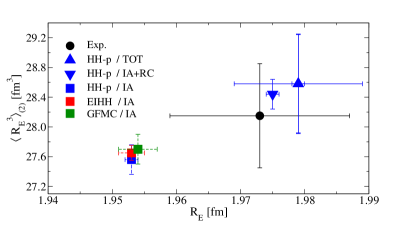
Figure 1: (Color online) Third Zemach moment vs charge radius of ³He: different calculations are compared with experimental data from Ref. Sick (2014). The calculations are based on the AV18+UIX nuclear potential and Kelly form factors. Results with the charge operator in IA are labeled with IA, and those with the addition of RC (and two-body currents) are labeled with IA+RC (TOT). IA and IA+RC results are shown with uncertainties from the computational methods alone, while the calculations labeled with “TOT” include also the chiral truncation error. See text for details.

In Fig. 2, we show the magnetic observables, namely $R_{Z}$ versus $R_{M}$, calculated with the HH-p method. Also in this case, we observe a correlation between the two observables. In particular, the IA over-estimates experiment, and RC have a smaller effect ($\sim 3\%$) than the two-body currents ($\sim 6\%$). Also in this case, once RC and two-body currents are included, theoretical results agree nicely with experiment. When the chiral truncation error is accounted for (again only in the point labeled with “TOT”), theory and experiment have comparable uncertainties.

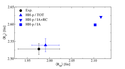
Figure 2: (Color online) First Zemach moment vs magnetic radius of ³He: various calculations are compared with experimental data from Ref. Sick (2014). Results with the charge operator in IA are labeled with IA, and those with the addition of RC (and two-body currents) are labeled with IA+RC (TOT). IA and IA+RC results are shown with uncertainties from the computational methods alone, while the calculations labeled with “TOT” include also the chiral truncation error. When not visible, error bars are included in the size of the symbols. See text for details.

III.3 Nuclear and nucleon models

At this point, we briefly address the dependency on variations in two inputs that were kept fixed until now, namely, the nuclear interaction and the nucleonic form factors. The effect due to a possible variance in each of these inputs may be considered as an additional source of uncertainty. To this end, we study the ${{\langle}{R^{3}_{E}}{\rangle}}_{(2)}$ and $R_{E}$ of ³He using the EIHH few-body method and the charge operator in IA.

Table 8: ³He electric moments in IA calculated with the EIHH method using i) either the AV18+UIX or the $\chi$EFT nuclear Hamiltonian, and ii) different parameterizations of the nucleonic form factor $G_{E}$. Quoted uncertainties include only the method and procedure error bars. Experimental values are from Ref. Sick (2014); Purcell et al. (2010). See text for details.

	$R_{E}$	${{\langle}{R^{3}_{E}}{\rangle}}_{(2)}$
Potential/$G_{E}$	[fm]	[fm3]
$\chi$EFT/CODATA	1.976(2)	28.33(14)
$\chi$EFT/Kelly	1.971(2)	28.20(14)
$\chi$EFT/CREMA	1.961(2)	27.72(14)
AV18+UIX/CODATA	1.958(2)	27.77(10)
AV18+UIX/Kelly	1.953(2)	27.65(10)
AV18+UIX/CREMA	1.943(2)	27.17(9)
Exp.	1.973(14)	28.15(70)

In order to provide a rough estimate of the overall nuclear model dependency, we simply repeat the calculations using a different nuclear Hamiltonian with two- and three-body interactions derived from chiral effective field theory. Following Refs. Ji et al. (2018); Nevo Dinur et al. (2016); Ji et al. (2013), we use the two- and three-body interactions derived in Refs. Entem and Machleidt (2003) and Navrátil (2007), respectively, and denote results from this Hamiltonian with “$\chi$EFT”. Results are shown in Table 8 for different potentials and also for different parameterization of the nucleonic form factor. If we use the same nucleon form factor as calculations in previous sections, namely the Kelly form factors, we see that the $\chi$EFT interactions shift the electric moments: both $R_{E}$ and ${{\langle}{R^{3}_{E}}{\rangle}}_{(2)}$ increase and agree better with the experimental values. The dynamical model dependency amounts to 1$\%$-2$\%$, which is compatible with the chiral truncation uncertainty estimate discussed before and is much larger than the sub-percentage few-body or procedure uncertainty.

The second variable input we address here is the specific parameterization of the nucleonic form factors. Our benchmark calculations are based on the Kelly parameterization, which is widely used due to its simplicity and high-quality fit of the available nucleon electromagnetic data. The Kelly parameterization yields a proton radius $r_{p}(K)=0.863(4)$ fm. Another common parameterization from global fits of electron scattering data is from Höhler Höhler et al. (1976). When tested in calculations of the electric moments of $A=3$ Piarulli et al. (2013), these parameterizations produce results in agreement at the sub-percent level.

Currently, the main uncertainty in this input pertains to the size of the proton, stemming from the discrepancy between the determination from muonic hydrogen by the CREMA collaboration Antognini et al. (2013), i.e., $r_{p}(\mu^{-})=0.84087(39)\ {\rm fm}$, and the most recent CODATA determination Mohr et al. (2016) of $r_{p}(e^{-})=0.8751(61)\ {\rm fm}$, which does not incorporate the muonic hydrogen result. In order to conservatively estimate the impact of this discrepancy at the nucleonic level onto nuclear observables, and in lack of parameterizations that account for this proton’s size uncertainty in the global fits, we adopt a simple parameterization. We the use dipole form to represent the nucleon form factor as was done, e.g., in Ref. Friar and Payne (2005), fitting the single parameter to reproduce either the CREMA or the CODATA proton radius. Clearly this approximation is completely driven by one observable at q=0, whereas the moments are, as we saw, sensitive to the slopes and shapes of the nucleonic form factors. With this warning in mind, we proceed our analysis. Following Ref. Ji et al. (2018), we take the neutron electric form factor to be of the modified Galster shape used in Friar and Payne (2005), updated to reproduce ${{\langle}{r^{2}_{E}}{\rangle}}_{n}=-0.116$ fm² from J. Beringer et al. (2012) (Particle Data Group).

Results for the charge radius and third Zemach moment are shown in Table 8, where we observe a 1$\%$–2$\%$ variance, which is as large as the dependency on the nuclear interaction. While the specific choice used of nuclear potential and nucleon form factors may significantly affect the perceived agreement of the IA calculation with experiment—e.g., the $\chi$EFT potential in combination with the Kelly or CODATA form factor is very close to the mean experimental value—we stress that RC and two-body currents are missing here. If one added consistently all the uncertainties stemming from the truncation in the chiral expansion, all these theoretical points would be statistically in agreement among themselves and with the experimental values–albeit with a slightly larger but comparable uncertainty.

Table 9: Uncertainty budget for the ³He electric moments. Experimental values are from Ref. Sick (2014); Purcell et al. (2010). See text for details.

	$\delta$(Method)	$\delta$(Dynamics)	$\delta$(FF)
$R_{E}$	0.1%	0.9%	0.8%
${{\langle}{R^{3}_{E}}{\rangle}}_{(2)}$	0.4-0.7%	2%	2.4%

Our findings are summarized in Table 9 where we show the uncertainty budget for these calculations. Here, $\delta$(Method) is the uncertainty from the few-body method and numerical procedure added in quadrature, $\delta$(Dynamics) is the model dependence accounted by testing two nuclear Hamiltonians, $\delta$(FF) is the sensitivity of our results to the use of this single nucleon input.

As already pointed out, $\delta$(Method) is small for $R_{E}$ and ${{\langle}{R^{3}_{E}}{\rangle}}_{(2)}$ and $\delta$(Dynamics) is of the same order as the chiral convergence uncertainty obtained by using the algorithm by Epelbaum et al. Epelbaum et al. (2015). Finally, $\delta$(FF) is roughly estimated using dipole form factors fixed to reproduce either the CREMA or the CODATA proton radii, giving a very conservative uncertainty, also the order of 1$\%$–2$\%$. It is to be noted that, e.g., the electric charge radii vary by only 0.15$\%$ when replacing Kelly nucleon form factors with a different global fit from Höhler et al. Höhler et al. (1976), as was done in Ref. Piarulli et al. (2013)

Overall, we observe that the uncertainty pertaining the nuclear dynamics and dipole nucleonic form factors are dominant over the method uncertainties.

IV Conclusions

In this paper, we performed benchmark calculations of electromagnetic moments relevant to ongoing experimental efforts, particularly those investigating the spectroscopy of muon-nucleus systems.

Benchmark calculations in IA are important to assess the reliability of the calculated electromagnetic moments within modern ab initio methods. We show that different few-body computational methods lead to compatible results, given the same dynamical inputs. We also investigated three distinct numerical procedures ($q$-space, $r$-space, and $qr$-space) that can be used to calculate these observables, and have shown that they yield comparable results in agreement at the 1$\%$ level or better, a part for the fourth electric moment, for which the $q$-space method produces a larger uncertainty.

The dominant source of uncertainty in the calculations is due to the employed dynamical inputs, that is, the nuclear Hamiltonian, the electromagnetic current operators, and the single nucleon parameterizations. In particular, few-body and numerical procedure errors are found to be at the sub-percent level in calculations of the ³He electric moments in IA based on the $r$-space procedure. The same observables have $\sim 1\%$–$2\%$ variation when different nuclear Hamiltonians are used.

We studied the RC and two-body current contributions in the $A=3$ systems using wave functions from the AV18+UIX Hamiltonian, and found that these contributions are important to reach agreement with the data. In particular, RC corrections are found to be relevant in electric moments, while two-body currents are necessary to explain magnetic data. The combined contribution from RC and two-body currents is at the $3\%$–$5\%$ level in $R_{E}$ and ${{\langle}{R^{3}_{E}}{\rangle}}_{(2)}$, and of the order of $\sim 3\%$–$6\%$ ($\sim 12\%$–$15\%$) in $R_{Z}$ and $R_{M}$ (the $A=3$ $\mu$’s). Lastly, in order to make contact with the CREMA findings on the proton’s size, and in order to asses the possible impact of these findings on nuclear observables, we used a dipole representation of the nucleonic form factors fitted to reproduce either the CREMA or the CODATA value. This produces yields a rather ample allowance for the uncertainty in the nucleonic input, and leads to a conservative few-percent error bar on the nuclear observables.

This first theoretical study of electromagnetic moments indicates that the total theoretical uncertainty is of the same order of magnitude as the experimental one at least for the charge, magnetic and Zemach radii, third Zemach moment, and magnetic moments. Finally, we remark that, while currently theoretical uncertainties seem comparable to those of electron scattering data, the anticipated precision of muonic experiments will be superior, further challenging the theory. Performing a fully consistent calculation accompanied by a thorough statistical and systematical analysis of these observables is demanding and will be explored in our future studies.

Acknowledgments – S.P. and M.P. would like to thank Rocco Schiavilla and Laura Elisa Marcucci for useful discussions, and gratefully acknowledge the computing resources of the high-performance computing cluster operated by the Laboratory Computing Resource Center (LCRC) at Argonne National Laboratory (ANL). This work was supported in parts by the Natural Sciences and Engineering Research Council (NSERC), the National Research Council of Canada, by the Deutsche Forschungsgemeinschaft DFG through the Collaborative Research Center [The Low-Energy Frontier of the Standard Model (SFB 1044)], and through the Cluster of Excellence [Precision Physics, Fundamental Interactions and Structure of Matter (PRISMA)]. The work of R.B.W. is supported by the U.S. Department of Energy, Office of Science, Office of Nuclear Physics, under Contract No. DE-AC02-06CH11357.

References

- Pohl et al. (2010) R. Pohl et al., Nature 466, 213 (2010).
- Antognini et al. (2013) A. Antognini et al., Science 339, 417 (2013).
- Pohl et al. (2016) R. Pohl, F. Nez, L. M. P. Fernandes, F. D. Amaro, F. Biraben, J. M. R. Cardoso, D. S. Covita, A. Dax, S. Dhawan, M. Diepold, A. Giesen, A. L. Gouvea, T. Graf, T. W. Hänsch, P. Indelicato, L. Julien, P. Knowles, F. Kottmann, E.-O. Le Bigot, Y.-W. Liu, J. A. M. Lopes, L. Ludhova, C. M. B. Monteiro, F. Mulhauser, T. Nebel, P. Rabinowitz, J. M. F. dos Santos, L. A. Schaller, K. Schuhmann, C. Schwob, D. Taqqu, J. F. C. A. Veloso, A. Antognini, and , Science 353, 669 (2016), http://science.sciencemag.org/content/353/6300/669.full.pdf .
- Pohl et al. (2017) R. Pohl, F. Nez, T. Udem, A. Antognini, A. Beyer, H. Fleurbaey, A. Grinin, T. W. Hänsch, L. Julien, F. Kottmann, J. J. Krauth, L. Maisenbacher, A. Matveev, and F. Biraben, Metrologia 54, L1 (2017).
- Bernauer and Pohl (2014) J. C. Bernauer and R. Pohl, Sci. Am. 310, 18 (2014).
- Pohl et al. (2013) R. Pohl, R. Gilman, G. A. Miller, and K. Pachucki, Ann. Rev. Nucl. Part. Sci. 63, 175 (2013), arXiv:1301.0905 [physics.atom-ph] .
- Beyer et al. (2017) A. Beyer et al., Science 358, 79 (2017).
- Fleurbaey et al. (2018) H. Fleurbaey et al., Phys. Rev. Lett. 120, 183001 (2018).
- (9) R. Pohl, F. Nez, L. M. P. Fernandes, M. A. Ahmed, F. D. Amaro, P. Amaro, F. Biraben, J. M. R. Cardoso, D. S. Covita, A. Dax, S. Dhawan, M. Diepold, B. Franke, S. Galtier, A. Giesen, A. L. Gouvea, J. Götzfried, T. Graf, T. W. Hänsch, M. Hildebrandt, P. Indelicato, L. Julien, K. Kirch, A. Knecht, P. Knowles, F. Kottmann, J. J. Krauth, E.-O. L. Bigot, Y.-W. Liu, J. A. M. Lopes, L. Ludhova, J. Machado, C. M. B. Monteiro, F. Mulhauser, T. Nebel, P. Rabinowitz, J. M. F. dos Santos, J. P. Santos, L. A. Schaller, K. Schuhmann, C. Schwob, C. I. Szabo, D. Taqqu, J. F. C. A. Veloso, A. Voss, B. Weichelt, and A. Antognini, “Laser spectroscopy of muonic atoms and ions,” in Proceedings of the 12th International Conference on Low Energy Antiproton Physics (LEAP2016), https://journals.jps.jp/doi/pdf/10.7566/JPSCP.18.011021 .
- Ji et al. (2018) C. Ji, S. Bacca, N. Barnea, O. J. Hernandez, and N. Nevo Dinur, Journal of Physics G: Nuclear and Particle Physics 45, 093002 (2018).
- Franke et al. (2017) B. Franke, J. J. Krauth, A. Antognini, M. Diepold, F. Kottmann, and R. Pohl, The European Physical Journal D 71, 341 (2017).
- Diepold et al. (2018) M. Diepold, B. Franke, J. J. Krauth, A. Antognini, F. Kottmann, and R. Pohl, Annals of Physics 396, 220 (2018).
- Eides et al. (2001) M. I. Eides, H. Grotch, and V. A. Shelyuto, Physics Reports 342, 63 (2001).
- Borie (2012) E. Borie, Annals of Physics 327, 733 (2012).
- Korzinin et al. (2018) E. Y. Korzinin, V. A. Shelyuto, V. G. Ivanov, and S. G. Karshenboim, Phys. Rev. A 97, 012514 (2018).
- Kalinowski et al. (2018) M. Kalinowski, K. Pachucki, and V. A. Yerokhin, (2018), arXiv:1810.06601 [physics.atom-ph] .
- Pachucki (2011) K. Pachucki, Phys. Rev. Lett. 106, 193007 (2011).
- Friar (2013) J. L. Friar, Phys. Rev. C 88, 034003 (2013).
- Ji et al. (2013) C. Ji, N. Nevo Dinur, S. Bacca, and N. Barnea, Phys. Rev. Lett. 111, 143402 (2013).
- Carlson et al. (2014) C. E. Carlson, M. Gorchtein, and M. Vanderhaeghen, Phys. Rev. A 89, 022504 (2014).
- Hernandez et al. (2014) O. Hernandez, C. Ji, S. Bacca, N. Nevo Dinur, and N. Barnea, Physics Letters B 736, 344 (2014).
- Pachucki and Wienczek (2015) K. Pachucki and A. Wienczek, Phys. Rev. A91, 040503 (2015), arXiv:1501.07451 [physics.atom-ph] .
- Nevo Dinur et al. (2016) N. Nevo Dinur, C. Ji, S. Bacca, and N. Barnea, Physics Letters B 755, 380 (2016).
- Carlson et al. (2017) C. E. Carlson, M. Gorchtein, and M. Vanderhaeghen, Phys. Rev. A95, 012506 (2017), arXiv:1611.06192 [nucl-th] .
- Kamada et al. (2001) H. Kamada et al., Phys. Rev. C64, 044001 (2001), arXiv:nucl-th/0104057 [nucl-th] .
- Viviani et al. (2017) M. Viviani, A. Deltuva, R. Lazauskas, A. C. Fonseca, A. Kievsky, and L. E. Marcucci, Phys. Rev. C 95, 034003 (2017).
- Lazauskas (2018) R. Lazauskas, Phys. Rev. C97, 044002 (2018), arXiv:1711.04716 [nucl-th] .
- Nevo Dinur et al. (2014) N. Nevo Dinur, N. Barnea, C. Ji, and S. Bacca, Phys. Rev. C 89, 064317 (2014).
- Baker et al. (2018) R. B. Baker, K. D. Launey, N. Nevo Dinur, S. Bacca, J. P. Draayer, and T. Dytrych, AIP Conference Proceedings 2038, 020006 (2018), https://aip.scitation.org/doi/pdf/10.1063/1.5078825 .
- Hartree (1958) D. R. Hartree, Numerical Analysis (Oxford University Press, 2nd ed., 1958).
- Hernandez et al. (2018) O. Hernandez, A. Ekström, N. Nevo Dinur, C. Ji, S. Bacca, and N. Barnea, Physics Letters B 778, 377 (2018).
- Wiringa (1991) R. B. Wiringa, Phys.Rev. C43, 1585 (1991).
- Pudliner et al. (1997) B. S. Pudliner, V. R. Pandharipande, J. Carlson, S. C. Pieper, and R. B. Wiringa, Phys. Rev. C 56, 1720 (1997).
- Piarulli et al. (2013) M. Piarulli, L. Girlanda, L. E. Marcucci, S. Pastore, R. Schiavilla, et al., Phys. Rev. C 87, 014006 (2013).
- Barnea et al. (2001) N. Barnea, W. Leidemann, and G. Orlandini, Nuclear Physics A 693, 565 (2001).
- Leidemann and Orlandini (2013) W. Leidemann and G. Orlandini, Prog.Part.Nucl.Phys. 68, 158 (2013).
- Bacca and Pastore (2014) S. Bacca and S. Pastore, J. Phys. G41, 123002 (2014), arXiv:1407.3490 [nucl-th] .
- Marcucci et al. (2016) L. E. Marcucci, F. Gross, M. T. Pena, M. Piarulli, R. Schiavilla, I. Sick, A. Stadler, J. W. Van Orden, and M. Viviani, J. Phys. G43, 023002 (2016), arXiv:1504.05063 [nucl-th] .
- Carlson and Schiavilla (1998) J. Carlson and R. Schiavilla, Rev. Mod. Phys. 70, 743 (1998).
- Kievsky et al. (2008a) A. Kievsky, S. Rosati, M. Viviani, L. E. Marcucci, and L. Girlanda, J. Phys. G35, 063101 (2008a), arXiv:0805.4688 [nucl-th] .
- Viviani et al. (2006) M. Viviani, L. E. Marcucci, S. Rosati, A. Kievsky, and L. Girlanda, Few Body Syst. 39, 159 (2006), arXiv:nucl-th/0512077 [nucl-th] .
- Phillips (2016) D. R. Phillips, Annual Review of Nuclear and Particle Science 66, 421 (2016), https://doi.org/10.1146/annurev-nucl-102014-022321 .
- Pastore et al. (2008) S. Pastore, R. Schiavilla, and J. L. Goity, Phys. Rev. C 78, 064002 (2008).
- Pastore et al. (2009) S. Pastore, L. Girlanda, R. Schiavilla, M. Viviani, and R. B. Wiringa, Phys. Rev. C 80, 034004 (2009).
- Pastore et al. (2011) S. Pastore, L. Girlanda, R. Schiavilla, and M. Viviani, Phys. Rev. C 84, 024001 (2011).
- Kolling et al. (2009) S. Kolling, E. Epelbaum, H. Krebs, and U.-G. Meißner, Phys. Rev. C 80, 045502 (2009).
- Kolling et al. (2011) S. Kolling, E. Epelbaum, H. Krebs, and U.-G. Meißner, Phys. Rev. C 84, 054008 (2011).
- Kolling et al. (2012) S. Kolling, E. Epelbaum, and D. R. Phillips, Phys. Rev. C86, 047001 (2012).
- Zemach (1956) A. C. Zemach, Phys. Rev. 104, 1771 (1956).
- Kelly (2004) J. J. Kelly, Phys. Rev. C 70, 068202 (2004).
- Wiringa et al. (1995) R. B. Wiringa, V. G. J. Stoks, and R. Schiavilla, Phys. Rev. C 51, 38 (1995).
- Pudliner et al. (1995) B. S. Pudliner, V. R. Pandharipande, J. Carlson, and R. B. Wiringa, Phys. Rev. Lett. 74, 4396 (1995).
- Mohr et al. (2016) P. J. Mohr, D. B. Newell, and B. N. Taylor, Rev. Mod. Phys. 88, 035009 (2016).
- Friar and Sick (2004) J. L. Friar and I. Sick, Physics Letters B 579, 285 (2004).
- Afanasev et al. (1998) A. V. Afanasev, V. D. Afanasev, and S. V. Trubnikov, arXiv:nucl-th/9808047 (1998).
- Sick (2014) I. Sick, Phys. Rev. C 90, 064002 (2014).
- Purcell et al. (2010) J. Purcell, J. Kelley, E. Kwan, C. Sheu, and H. Weller, Nuclear Physics A 848, 1 (2010).
- Angeli and Marinova (2013) I. Angeli and K. Marinova, Atomic Data and Nuclear Data Tables 99, 69 (2013).
- Schiavilla et al. (2018) R. Schiavilla et al., (2018), arXiv:1809.10180 [nucl-th] .
- Kievsky et al. (2008b) A. Kievsky, S. Rosati, M. Viviani, L. E. Marcucci, and L. Girlanda, Journal of Physics G: Nuclear and Particle Physics 35, 063101 (2008b).
- Pieper et al. (2001) S. C. Pieper, V. R. Pandharipande, R. B. Wiringa, and J. Carlson, Phys. Rev. C 64, 014001 (2001).
- Epelbaum et al. (2015) E. Epelbaum, H. Krebs, and U.-G. Meissner, The European Physical Journal A 51, 53 (2015).
- Entem and Machleidt (2003) D. R. Entem and R. Machleidt, Phys. Rev. C 68, 041001 (2003).
- Navrátil (2007) P. Navrátil, Few-Body Systems 41, 117 (2007).
- Höhler et al. (1976) G. Höhler, E. Pietarinen, I. Sabba-Stefanescu, F. Borkowski, G. Simon, V. Walther, and R. Wendling, Nuclear Physics B 114, 505 (1976).
- Friar and Payne (2005) J. L. Friar and G. L. Payne, Phys. Rev. C 72, 014002 (2005).
- J. Beringer et al. (2012) (Particle Data Group) J. Beringer et al. (Particle Data Group), Phys. Rev. D 86, 010001 (2012).