Analysis of a projection method for the Stokes problem using an $\varepsilon$-Stokes approach

Abstract

We generalize pressure boundary conditions of an $\varepsilon$-Stokes problem. Our $\varepsilon$-Stokes problem connects the classical Stokes problem and the corresponding pressure-Poisson equation using one parameter $\varepsilon>0$. For the Dirichlet boundary condition, it is proven in K. Matsui and A. Muntean (2018) that the solution for the $\varepsilon$-Stokes problem converges to the one for the Stokes problem as $\varepsilon$ tends to 0, and to the one for the pressure-Poisson problem as $\varepsilon$ tends to $\infty$. Here, we extend these results to the Neumann and mixed boundary conditions. We also establish error estimates in suitable norms between the solutions to the $\varepsilon$-Stokes problem, the pressure-Poisson problem and the Stokes problem, respectively. Several numerical examples are provided to show that several such error estimates are optimal in $\varepsilon$. Our error estimates are improved if one uses the Neumann boundary conditions. In addition, we show that the solution to the $\varepsilon$-Stokes problem has a nice asymptotic structure.

1 Introduction

Let $\Omega$ be a bounded domain in ${\mathbb{R}}^{n}(n\geq 2,n\in{\mathbb{N}})$ with Lipschitz continuous boundary $\Gamma$ and let $F:\Omega\rightarrow{\mathbb{R}}^{n}$ be a given applied force field and $u_{b}:\Gamma\rightarrow{\mathbb{R}}^{n}$ be a given Dirichlet boundary data satisfying $\int_{\Gamma}u_{b}\cdot\nu=0$, where $\nu$ is the unit outward normal vector on $\Gamma$. A strong form of the Stokes problem is given as follows. Find $u_{\mbox{\tiny$S$}}:\Omega\rightarrow{\mathbb{R}}^{n}$ and $p_{\mbox{\tiny$S$}}:\Omega\rightarrow{\mathbb{R}}$ such that

$$\left\{\begin{array}[]{ll}-\Delta u_{\mbox{\tiny$S$}}+\nabla p_{\mbox{\tiny$S$}}=F&\mbox{in }\Omega,\\ {\operatorname{div}}u_{\mbox{\tiny$S$}}=0&\mbox{in }\Omega,\\ u_{\mbox{\tiny$S$}}=u_{b}&\mbox{on }\Gamma,\end{array}\right.$$ (1.4)

where $u_{\mbox{\tiny$S$}}$ and $p_{\mbox{\tiny$S$}}$ are the velocity and the pressure of the flow governed by (S), respectively. We refer to Temam for the details on the Stokes problem (i.e., physical background and corresponding mathematical analysis). Taking the divergence of the first equation, we obtain

$${\operatorname{div}}F={\operatorname{div}}(-\Delta u_{\mbox{\tiny$S$}}+\nabla p_{\mbox{\tiny$S$}})=-\Delta({\operatorname{div}}u_{\mbox{\tiny$S$}})+\Delta p_{\mbox{\tiny$S$}}=\Delta p_{\mbox{\tiny$S$}}.$$ (1.5)

This equation is often called the pressure-Poisson equation and is used in numerical schemes such as MAC (marker and cell), SMAC (simplified MAC) and the projection methods (see, e.g., Amsden_Harlow ; Chorin68 ; Cummins_Rudman ; Guermond ; mac1 ; Kim_Moin ; mac2 ; Perot ). Based on the above, we consider a similar problem. Find $u_{\mbox{\tiny$P\!P$}}:\Omega\rightarrow{\mathbb{R}}^{n}$ and $p_{\mbox{\tiny$P\!P$}}:\Omega\rightarrow{\mathbb{R}}$ satisfying

$$\left\{\begin{array}[]{ll}-\Delta u_{\mbox{\tiny$P\!P$}}+\nabla p_{\mbox{\tiny$P\!P$}}=F&\mbox{in }\Omega,\\ -\Delta p_{\mbox{\tiny$P\!P$}}=-{\operatorname{div}}F&\mbox{in }\Omega,\\ u_{\mbox{\tiny$P\!P$}}=u_{b}&\mbox{on }\Gamma,\\ +\mbox{boundary condition for }p_{\mbox{\tiny$P\!P$}}.&\end{array}\right.$$ (1.10)

We call this problem the pressure-Poisson problem. The idea of using (1.5) instead of ${\operatorname{div}}u_{\mbox{\tiny$S$}}=0$ is useful for calculating the pressure numerically in the Navier–Stokes equation. For example, this idea is used in MAC, SMAC and projection methods. The Dirichlet boundary condition for the pressure is used in an outflow boundary Chan_Street ; Viecelli . See also Conca_etc94 ; Conca_etc95 ; Marusic .

We introduce an “interpolation” between problems (S) and (PP). For $\varepsilon>0$, find $u_{\varepsilon}:\Omega\rightarrow{\mathbb{R}}^{n}$ and $p_{\varepsilon}:\Omega\rightarrow{\mathbb{R}}$ such that

$$\left\{\begin{array}[]{ll}-\Delta u_{\varepsilon}+\nabla p_{\varepsilon}=F&\mbox{in }\Omega,\\ -\varepsilon\Delta p_{\varepsilon}+{\operatorname{div}}u_{\varepsilon}=-\varepsilon{\operatorname{div}}F&\mbox{in }\Omega,\\ u_{\varepsilon}=u_{b}&\mbox{on }\Gamma,\\ +\mbox{boundary condition for }p_{\varepsilon}.&\end{array}\right.$$ (1.15)

This problem is called the $\varepsilon$-Stokes problem (ES) in prev . In Douglas_Wang ; Glowinski ; Hughes , the authors treat this problem as an approximation of the Stokes problem to avoid numerical instabilities. The $\varepsilon$-Stokes problem approximates the Stokes problem (S) as $\varepsilon\rightarrow 0$ and the pressure-Poisson problem (PP) as $\varepsilon\rightarrow\infty$ (Fig. 1). It is shown in prev that if $p_{\mbox{\tiny$S$}}\in{H^{1}(\Omega)}$ then there exists a constant $c>0$ independent of $\varepsilon$ such that

$$\begin{array}[]{rrl}\|u_{\mbox{\tiny$S$}}-u_{\mbox{\tiny$P\!P$}}\|_{{H^{1}(\Omega)}^{n}}&\leq&c\|\gamma_{0}p_{\mbox{\tiny$S$}}-\gamma_{0}p_{\mbox{\tiny$P\!P$}}\|_{H^{1/2}(\Gamma)},\\ \|u_{\mbox{\tiny$S$}}-u_{\varepsilon}\|_{{H^{1}(\Omega)}^{n}}&\leq&c\|\gamma_{0}p_{\mbox{\tiny$S$}}-\gamma_{0}p_{\mbox{\tiny$P\!P$}}\|_{H^{1/2}(\Gamma)},\end{array}$$

where $\gamma_{0}\in B({H^{1}(\Omega)},H^{1/2}(\Gamma))$ is the standard trace operator Girault . From the first inequality, if we have a good prediction value for pressure on $\Gamma$, then $u_{\mbox{\tiny$P\!P$}}$ is a good approximation of $u_{\mbox{\tiny$S$}}$. Moreover, $u_{\varepsilon}$ is also a good approximation of $u_{\mbox{\tiny$S$}}$ from the second inequality.

Figure 1: Sketch of the connections between the problems (S), (PP) and (ES).

Next we specify the boundary conditions for $p_{\mbox{\tiny$P\!P$}}$ and $p_{\varepsilon}$. We assume that the boundary $\Gamma$ is a union of two open subsets $\Gamma_{D}$ and $\Gamma_{N}$ such that

$$|\Gamma\setminus(\Gamma_{D}\cup\Gamma_{N})|=0,\quad|\Gamma_{D}|>0,\quad\Gamma_{D}\cap\Gamma_{N}=\emptyset,$$

and number of connected components of $\Gamma_{D}$ and $\Gamma_{N}$ with respect to the relative topology of $\Gamma$ are finite. We consider a Neumann boundary condition (1.16) and a mixed boundary condition (1.21),

$${\displaystyle\frac{\partial p_{\mbox{\tiny$P\!P$}}}{\partial\nu}=g_{b}}\mbox{ on }\Gamma,\quad{\displaystyle\frac{\partial p_{\varepsilon}}{\partial\nu}=g_{b}}\mbox{ on }\Gamma,$$ (1.16)

$$\left\{\begin{array}[]{ll}p_{\mbox{\tiny$P\!P$}}=p_{b}&\mbox{on }\Gamma_{D},\\[8.0pt] {\displaystyle\frac{\partial p_{\mbox{\tiny$P\!P$}}}{\partial\nu}=g_{b}}&\mbox{on }\Gamma_{N},\end{array}\right.\quad\left\{\begin{array}[]{ll}p_{\varepsilon}=p_{b}&\mbox{on }\Gamma_{D},\\[8.0pt] {\displaystyle\frac{\partial p_{\varepsilon}}{\partial\nu}=g_{b}}&\mbox{on }\Gamma_{N},\end{array}\right.$$ (1.21)

where $p_{b}:\Gamma_{D}\rightarrow{\mathbb{R}}$ and $g_{b}=\Gamma\rightarrow{\mathbb{R}}$ satisfying $\int_{\Gamma}g_{b}=\int_{\Gamma}{\operatorname{div}}F$ are given boundary data.

In prev , the authors impose Dirichlet boundary conditions for $p_{\mbox{\tiny$P\!P$}}$ and $p_{\varepsilon}$ (i.e., (1.21) with $\Gamma_{D}=\Gamma$ and $\Gamma_{N}=\emptyset$.) For such boundary conditions, they introduce a weak solution $(u_{\varepsilon},p_{\varepsilon})$ to the $\varepsilon$-Stokes problem (ES) and prove that $(u_{\varepsilon},p_{\varepsilon})$ strongly converges in ${H^{1}(\Omega)}^{n}\times{H^{1}(\Omega)}$ to a weak solution to the pressure-Poisson problem (PP) as $\varepsilon\rightarrow\infty$ and weakly converges in ${H^{1}_{0}(\Omega)}^{n}\times({L^{2}(\Omega)}/{\mathbb{R}})$ to a weak solution $(u_{\mbox{\tiny$S$}},p_{\mbox{\tiny$S$}})$ to the Stokes problem (S) as $\varepsilon\rightarrow 0$. Moreover, if $p_{\mbox{\tiny$S$}}\in{H^{1}(\Omega)}$, then strong convergence of $(u_{\varepsilon},p_{\varepsilon})$ to $(u_{\mbox{\tiny$S$}},p_{\mbox{\tiny$S$}})$ as $\varepsilon\rightarrow 0$ holds.

In this paper, we generalize the Dirichlet boundary condition of $p_{\mbox{\tiny$P\!P$}}$ and $p_{\varepsilon}$ to both the Neumann boundary condition (1.16) and the mixed boundary condition (1.21), and prove the corresponding convergence result (see Theorem 3.1, 4.2 and 4.3). Since the mixed boundary condition for pressure often appears in engineering problems, this generalization of the boundary conditions for pressure is important. In addition, for the Neumann boundary condition, we estimate the error between the weak solutions to (ES) and (S) provided $p_{\mbox{\tiny$S$}}\in{H^{1}(\Omega)}$. We also give an asymptotic expansion for the weak solution to (ES). We furthermore check this convergence result using numerical computations.

The organization of this paper is as follows. In Section 2 we introduce the notation used in this work and the weak form of these problems. We also prove the well-posedness of the problems (PP) and (ES) and show some their properties. In Section 3 we study that the solution to (ES) converges to the solution to (PP) in the strong topology as $\varepsilon\rightarrow\infty$. We also explore here the structure of the regular perturbation asymptotics. Section 4 is devoted to proving that the solution to (ES) converges to the solution to (S) in the weak and strong topology as $\varepsilon\rightarrow 0$. Finally, in Section 5, we show several numerical examples of these problems. The numerical errors between the problems (ES) and (PP), and between the problems (ES) and (S) using the P2/P1 finite element method. Proofs for several theorems which are similar to ones in prev are described.

2 Well-posedness

In this section, we introduce the notation and the weak form of the problems (S), (PP) and (ES), and prove their well-posedness. We give estimates between these solutions by using a pressure error on the boundary $\Gamma$.

2.1 Notation

We set

$$\begin{array}[]{ll}C^{\infty}_{0}(\Omega)^{n}&{\displaystyle:=\{\varphi\in C^{\infty}(\Omega)^{n}\,|\,\mbox{supp}(\varphi)\subset\Omega\},}\\[8.0pt] {L^{2}(\Omega)}/{\mathbb{R}}&:={\displaystyle\left\{\psi\in{L^{2}(\Omega)}\,\middle|\,\int_{\Omega}\psi=0\right\},}\\[8.0pt] {H^{1}(\Omega)}/{\mathbb{R}}&:={H^{1}(\Omega)}\cap({L^{2}(\Omega)}/{\mathbb{R}}),\\[8.0pt] {H^{1}_{0,D}(\Omega)}&:={\displaystyle\{\psi\in{H^{1}(\Omega)}\mid\psi|_{\Gamma_{D}}=0\}.}\\[8.0pt] \end{array}$$

For $m\in{\mathbb{N}}$, ${H^{-1}(\Omega)}^{m}:=({H^{1}_{0}(\Omega)}^{m})^{*}$ is equipped with the dual norm

$$\|f\|_{{H^{-1}(\Omega)}^{m}}:=\sup_{\varphi\in S_{m}}\langle f,\varphi\rangle\mbox{ for }f\in{H^{-1}(\Omega)}^{m},$$

where

$$S_{m}:=\{\varphi\in{H^{1}_{0}(\Omega)}^{m}~{}|~{}\|\nabla\varphi\|_{{L^{2}(\Omega)}^{n\times m}}=1\}.$$

Let $Q\subset{H^{1}(\Omega)}$ be a closed subspace such that there exists a constant $c>0$ for which $\|q\|_{L^{2}(\Omega)}\leq c\|\nabla q\|_{{L^{2}(\Omega)}^{n}}$ for all $q\in Q$. The dual space $Q^{*}$ is equipped with the norm

$$\|f\|_{Q^{*}}:=\sup_{\psi\in S_{Q}}\langle f,\psi\rangle$$

for $f\in Q^{*}$, where

$$S_{Q}:=\{\psi\in Q~{}|~{}\|\nabla\psi\|_{{L^{2}(\Omega)}^{n}}=1\}.$$

We define

$$\begin{array}[]{rl}[p]&:={\displaystyle p-\frac{1}{|\Omega|}\int_{\Omega}p,}\\[8.0pt] \|p\|_{{L^{2}(\Omega)}/{\mathbb{R}}}&:={\displaystyle\inf_{a\in{\mathbb{R}}}\|p-a\|_{L^{2}(\Omega)}=\|[p]\|_{L^{2}(\Omega)},}\\[8.0pt] \langle\nabla p,\varphi\rangle&:={\displaystyle-\int_{\Omega}p\,{\operatorname{div}}\varphi}\\[8.0pt] {\displaystyle\nabla u:\nabla\varphi}&:={\displaystyle\sum^{n}_{i=1}\frac{\partial u}{\partial x_{i}}\cdot\frac{\partial\varphi}{\partial x_{i}}}\end{array}$$

for all $p\in{L^{2}(\Omega)},u,\varphi\in{H^{1}_{0}(\Omega)}^{n}$, where $|\Omega|$ is the volume of $\Omega$.

2.2 Preliminary results

Let $\gamma_{0}\in B({H^{1}(\Omega)},H^{1/2}(\Gamma))$ be the standard trace operator. The trace operator $\gamma_{0}$ is surjective and satisfies $\mbox{Ker}(\gamma_{0})={H^{1}_{0}(\Omega)}$ (Girault, , Theorem 1.5). Let $\nu$ be the unit outward normal for $\Gamma$. Since $\nu$ is a unit vector, ${H^{1}(\Omega)}^{3}\ni u\mapsto u\cdot\nu:=(\gamma_{0}u)\cdot\nu\in H^{1/2}(\Gamma)$ is a linear continuous map. For all $u\in{H^{1}(\Omega)}^{3}$ and $\omega\in{H^{1}(\Omega)}$, the following Gauss divergence formula holds:

$$\int_{\Omega}u\cdot\nabla\omega+\int_{\Omega}({\operatorname{div}}u)\omega=\int_{\Gamma}(u\cdot\nu)\omega.$$

We recall the following four embedding theorems which plays an important role in the proof of the existence of pressure solutions to the Stokes problem. For the proof of Theorem 2.1, see (Necas, , Lemma 7.1) and (Duvaut, , Theorem 3.2 and Remark 3.1).

Theorem 2.1

There exists a constant $c>0$ such that

$$\|f\|_{L^{2}(\Omega)}\leq c(\|f\|_{H^{-1}(\Omega)}+\|\nabla f\|_{{H^{-1}(\Omega)}^{n}})$$

for all $f\in{L^{2}(\Omega)}$.

The following result follows from Theorem 2.1.

Theorem 2.2

(Girault, , Corollary 2.1, 2^∘) There exists a constant $c>0$ such that

$$\|f\|_{{L^{2}(\Omega)}/{\mathbb{R}}}\leq c\|\nabla f\|_{{H^{-1}(\Omega)}^{n}}$$

for all $f\in{L^{2}(\Omega)}$.

The following two embedding theorems are often called the Poincaré inequality.

Theorem 2.3

(Necas, , Theorem 7.8) There exists a constant $c>0$ such that

$$\|\psi\|_{L^{2}(\Omega)}\leq c\|\nabla\psi\|_{{L^{2}(\Omega)}^{n}}$$

for all $\psi\in{H^{1}(\Omega)}/{\mathbb{R}}$.

Theorem 2.4

(Girault, , Lemma 3.1) There exists a constant $c>0$ such that

$$\|\psi\|_{L^{2}(\Omega)}\leq c\|\nabla\psi\|_{{L^{2}(\Omega)}^{n}}$$

for all $\psi\in{H^{1}_{0,D}(\Omega)}$.

2.3 Weak formulations of the problems (PP), (S) and (ES)

We assume the following conditions for $F,u_{b}$ and $g_{b}$:

$$F\in{L^{2}(\Omega)}^{n},\quad u_{b}\in H^{1/2}(\Gamma),\quad\int_{\Gamma}u_{b}\cdot\nu=0,$$ (2.22)

$$g_{b}\in L^{2}(\Gamma),\quad{\operatorname{div}}F\in{L^{2}(\Omega)},$$ (2.23)

$$\int_{\Gamma}g_{b}=\int_{\Omega}{\operatorname{div}}F,$$ (2.24)

$$p_{b}\in{H^{1}(\Omega)}.$$ (2.25)

We start by defining the weak solution to (S). For all $\varphi\in{H^{1}_{0}(\Omega)}^{n}$, we obtain from the first equation of (S) that

$$\int_{\Omega}F\cdot\varphi=-\int_{\Gamma}\frac{\partial u_{\mbox{\tiny$S$}}}{\partial\nu}\cdot\varphi+\int_{\Omega}\nabla u_{\mbox{\tiny$S$}}:\nabla\varphi+\int_{\Omega}\nabla p_{\mbox{\tiny$S$}}\cdot\varphi=\int_{\Omega}\nabla u_{\mbox{\tiny$S$}}:\nabla\varphi+\int_{\Omega}\nabla p_{\mbox{\tiny$S$}}\cdot\varphi.$$

Using this expression, the weak form of the Stokes problem becomes as follows: Find $u_{\mbox{\tiny$S$}}\in{H^{1}(\Omega)}^{n}$ and $p_{\mbox{\tiny$S$}}\in{L^{2}(\Omega)}/{\mathbb{R}}$ such that

$$\left\{\begin{array}[]{ll}{\displaystyle\int_{\Omega}\nabla u_{\mbox{\tiny$S$}}:\nabla\varphi+\langle\nabla p_{\mbox{\tiny$S$}},\varphi\rangle=\int_{\Omega}F\cdot\varphi}&\mbox{for all }\varphi\in{H^{1}_{0}(\Omega)}^{n},\\[8.0pt] {\operatorname{div}}u_{\mbox{\tiny$S$}}=0&\mbox{in }{L^{2}(\Omega)},\\ u_{\mbox{\tiny$S$}}=u_{b}&\mbox{in }H^{1/2}(\Gamma)^{n}.\end{array}\right.$$ (2.29)

Next, we define the weak formulations of (PP) and (ES) first for the Neumann boundary condition (1.16) and them for the mixed boundary condition (1.21). After that, we define generalized weak formulations for (PP) and (ES) which cover both cases.

First, we apply the Neumann boundary condition (1.16) for (PP) and (ES). We take a test function $\psi\in{H^{1}(\Omega)}$. From the second equation of (PP), we obtain

$$\begin{array}[]{ll}{\displaystyle-\int_{\Omega}({\operatorname{div}}F)\psi}&{\displaystyle=-\int_{\Omega}(\Delta p_{\mbox{\tiny$P\!P$}})\psi}={\displaystyle-\int_{\Gamma}\frac{\partial p_{\mbox{\tiny$P\!P$}}}{\partial\nu}\psi+\int_{\Omega}\nabla p_{\mbox{\tiny$P\!P$}}\cdot\nabla\psi}\\[8.0pt] &{\displaystyle=-\int_{\Gamma}g_{b}\psi+\int_{\Omega}\nabla p_{\mbox{\tiny$P\!P$}}\cdot\nabla\psi}.\end{array}$$

Hence,

$$\int_{\Omega}\nabla p_{\mbox{\tiny$P\!P$}}\cdot\nabla\psi=\int_{\Gamma}g_{b}\psi-\int_{\Omega}({\operatorname{div}}F)\psi.$$

We note that $\int_{\Gamma}g_{b}\psi-\int_{\Omega}({\operatorname{div}}F)\psi=\int_{\Gamma}g_{b}[\psi]-\int_{\Omega}({\operatorname{div}}F)[\psi]$ for all $\psi\in{H^{1}(\Omega)}$ by (2.24). Therefore, the weak form of the pressure-Poisson problem with the Neumann boundary condition (1.16) becomes as follows. Find $u_{\mbox{\tiny$P\!P$}}\in{H^{1}(\Omega)}^{n}$ and $p_{\mbox{\tiny$P\!P$}}\in{H^{1}(\Omega)}/{\mathbb{R}}$ such that

$$\left\{\begin{array}[]{ll}{\displaystyle\int_{\Omega}\nabla u_{\mbox{\tiny$P\!P$}}:\nabla\varphi+\int_{\Omega}\nabla p_{\mbox{\tiny$P\!P$}}\cdot\varphi=\int_{\Omega}F\cdot\varphi}&\mbox{for all }\varphi\in{H^{1}_{0}(\Omega)}^{n},\\[8.0pt] {\displaystyle\int_{\Omega}\nabla p_{\mbox{\tiny$P\!P$}}\cdot\nabla\psi=\langle G_{1},\psi\rangle}&\mbox{for all }\psi\in{H^{1}(\Omega)}/{\mathbb{R}},\\ u_{\mbox{\tiny$P\!P$}}=u_{b}&\mbox{in }H^{1/2}(\Gamma)^{n},\end{array}\right.$$ (2.33)

where $G_{1}\in{H^{1}(\Omega)}^{*}$ such that $\langle G_{1},\psi\rangle=\int_{\Gamma}g_{b}\psi-\int_{\Omega}({\operatorname{div}}F)\psi~{}(\psi\in{H^{1}(\Omega)})$.

The weak form of (ES) with the Neumann boundary condition can be defined similarly to that of (PP). Find $u_{\varepsilon}\in{H^{1}(\Omega)}^{n}$ and $p_{\varepsilon}\in{H^{1}(\Omega)}/{\mathbb{R}}$ such that

$$\left\{\begin{array}[]{ll}{\displaystyle\int_{\Omega}\nabla u_{\varepsilon}:\nabla\varphi+\int_{\Omega}\nabla p_{\varepsilon}\cdot\varphi=\int_{\Omega}F\cdot\varphi}&\mbox{for all }\varphi\in{H^{1}_{0}(\Omega)}^{n},\\[8.0pt] {\displaystyle\varepsilon\int_{\Omega}\nabla p_{\varepsilon}\cdot\nabla\psi+\int_{\Omega}({\operatorname{div}}u_{\varepsilon})\psi=\varepsilon\langle G_{1},\psi\rangle}&\mbox{for all }\psi\in{H^{1}(\Omega)}/{\mathbb{R}},\\ u_{\mbox{\tiny$S$}}=u_{b}&\mbox{in }H^{1/2}(\Gamma)^{n}.\end{array}\right.$$ (2.37)

Secondly, we apply the mixed boundary condition (1.21) for (PP) and (ES). We take a test function $\psi\in{H^{1}_{0,D}(\Omega)}$. From the second equation of (PP), we obtain

$$\begin{array}[]{ll}{\displaystyle-\int_{\Omega}({\operatorname{div}}F)\psi}&{\displaystyle=-\int_{\Omega}(\Delta p_{\mbox{\tiny$P\!P$}})\psi}={\displaystyle-\int_{\Gamma}\frac{\partial p_{\mbox{\tiny$P\!P$}}}{\partial\nu}\psi+\int_{\Omega}\nabla p_{\mbox{\tiny$P\!P$}}\cdot\nabla\psi}\\[8.0pt] &{\displaystyle=-\int_{\Gamma_{N}}g_{b}\psi+\int_{\Omega}\nabla p_{\mbox{\tiny$P\!P$}}\cdot\nabla\psi}.\end{array}$$

Hence,

$$\int_{\Omega}\nabla p_{\mbox{\tiny$P\!P$}}\cdot\nabla\psi=\int_{\Gamma_{N}}g_{b}\psi-\int_{\Omega}({\operatorname{div}}F)\psi.$$

The weak form of the pressure-Poisson problem with the mixed boundary condition (1.21) becomes as follows. Find $u_{\mbox{\tiny$P\!P$}}\in{H^{1}(\Omega)}^{n}$ and $p_{\mbox{\tiny$P\!P$}}\in{H^{1}(\Omega)}$ such that

$$\left\{\begin{array}[]{ll}{\displaystyle\int_{\Omega}\nabla u_{\mbox{\tiny$P\!P$}}:\nabla\varphi+\int_{\Omega}\nabla p_{\mbox{\tiny$P\!P$}}\cdot\varphi=\int_{\Omega}F\cdot\varphi}&\mbox{for all }\varphi\in{H^{1}_{0}(\Omega)}^{n},\\[8.0pt] {\displaystyle\int_{\Omega}\nabla p_{\mbox{\tiny$P\!P$}}\cdot\nabla\psi=\langle G_{2},\psi\rangle}&\mbox{for all }\psi\in{H^{1}_{0,D}(\Omega)},\\ u_{\mbox{\tiny$P\!P$}}=u_{b}&\mbox{in }H^{1/2}(\Gamma)^{n},\\ p_{\mbox{\tiny$P\!P$}}=p_{b}&\mbox{in }H^{1/2}(\Gamma_{D}),\end{array}\right.$$ (2.42)

where $G_{2}\in{H^{1}_{0,D}(\Omega)}^{*}$ such that

$$\langle G_{2},\psi\rangle=\int_{\Gamma_{N}}g_{b}\psi-\int_{\Omega}({\operatorname{div}}F)\psi$$

for $\psi\in{H^{1}_{0,D}(\Omega)}$. The weak form of (ES) with the mixed boundary condition (1.21) can be defined similarly to that of (PP). It reads as follows. Find $u_{\varepsilon}\in{H^{1}(\Omega)}^{n}$ and $p_{\varepsilon}\in{H^{1}(\Omega)}$ such that

$$\left\{\begin{array}[]{ll}{\displaystyle\int_{\Omega}\nabla u_{\varepsilon}:\nabla\varphi+\int_{\Omega}\nabla p_{\varepsilon}\cdot\varphi=\int_{\Omega}F\cdot\varphi}&\mbox{for all }\varphi\in{H^{1}_{0}(\Omega)}^{n},\\[8.0pt] {\displaystyle\varepsilon\int_{\Omega}\nabla p_{\varepsilon}\cdot\nabla\psi+\int_{\Omega}({\operatorname{div}}u_{\varepsilon})\psi=\varepsilon\langle G_{2},\psi\rangle}&\mbox{for all }\psi\in{H^{1}_{0,D}(\Omega)},\\ u_{\mbox{\tiny$S$}}=u_{b}&\mbox{in }H^{1/2}(\Gamma)^{n},\\ p_{\mbox{\tiny$S$}}=p_{b}&\mbox{in }H^{1/2}(\Gamma_{D}).\end{array}\right.$$ (2.47)

Finally, we generalize (PP₁) and (PP₂) to an abstract pressure-Poisson problem. Let $Q\subset{H^{1}(\Omega)}$ be a closed subspace as defined in Section 2.1. Find $u_{\mbox{\tiny$P\!P$}}\in{H^{1}(\Omega)}^{n}$ and $p_{\mbox{\tiny$P\!P$}}\in Q$ such that

$$\left\{\begin{array}[]{ll}{\displaystyle\int_{\Omega}\nabla u_{\mbox{\tiny$P\!P$}}:\nabla\varphi+\int_{\Omega}\nabla p_{\mbox{\tiny$P\!P$}}\cdot\varphi=\int_{\Omega}F\cdot\varphi}&{\rm\mbox{for all }}\varphi\in{H^{1}_{0}(\Omega)}^{n},\\[8.0pt] {\displaystyle\int_{\Omega}\nabla p_{\mbox{\tiny$P\!P$}}\cdot\nabla\psi=\langle G,\psi\rangle}&{\rm\mbox{for all }}\psi\in Q,\\ u_{\mbox{\tiny$P\!P$}}=u_{b}&\mbox{in }H^{1/2}(\Gamma)^{n},\\ p_{\mbox{\tiny$P\!P$}}-p_{b}\in Q,&\end{array}\right.$$ (2.52)

with $G\in Q^{*}$. Indeed, by Theorem 2.3 and 2.4, we obtain (PP₁) from (PP’) by putting $Q:={H^{1}(\Omega)}/{\mathbb{R}}$ and $G:=G_{1}$. Similarly, we obtain (PP₂) from (PP’) by putting $Q:={H^{1}_{0,D}(\Omega)}$ and $G:=G_{2}$.

We generalize (ES₁) and (ES₂) to an abstract $\varepsilon$-Stokes problem. Find $u_{\varepsilon}\in{H^{1}(\Omega)}^{n}$ and $p_{\varepsilon}\in Q$ such that

$$\left\{\begin{array}[]{ll}{\displaystyle\int_{\Omega}\nabla u_{\varepsilon}:\nabla\varphi+\int_{\Omega}\nabla p_{\varepsilon}\cdot\varphi=\int_{\Omega}F\cdot\varphi}&{\rm\mbox{for all }}\varphi\in{H^{1}_{0}(\Omega)}^{n},\\[8.0pt] {\displaystyle\varepsilon\int_{\Omega}\nabla p_{\varepsilon}\cdot\nabla\psi+\int_{\Omega}({\operatorname{div}}u_{\varepsilon})\psi=\varepsilon\langle G,\psi\rangle}&{\rm\mbox{for all }}\psi\in Q,\\ u_{\varepsilon}-u_{b}\in{H^{1}_{0}(\Omega)}^{n},&\\ p_{\varepsilon}-p_{b}\in Q.&\end{array}\right.$$ (2.57)

Indeed, by Theorem 2.3, 2.4, we obtain (ES₁) from (ES’) by putting $Q:={H^{1}(\Omega)}/{\mathbb{R}}$ and $G:=G_{1}$. Similarly, we also obtain (ES₂) from (ES’) by putting $Q:={H^{1}_{0,D}(\Omega)}$ and $G:=G_{2}$.

2.4 Well-posedness of (S’), (PP’) and (ES’)

We show the well-posedness of problems (S’), (PP’) and (ES’) in Theorem 2.5, 2.6 and 2.7.

Theorem 2.5

Under the condition (2.22), there exists a unique solution

$(u_{\mbox{\tiny$S$}},p_{\mbox{\tiny$S$}})\in{H^{1}(\Omega)}^{n}\times({L^{2}(\Omega)}/{\mathbb{R}})$ satisfying (S’).

See (Temam, , Theorem 2.4 and Remark 2.5) for the proof.

Theorem 2.6

Under the condition (2.22) and (2.25), for $G\in Q^{*}$, there exists a unique solution $(u_{\mbox{\tiny$P\!P$}},p_{\mbox{\tiny$P\!P$}})\in{H^{1}(\Omega)}^{n}\times Q$ satisfying (PP’).

Proof. Using the Lax–Milgram theorem, since $Q\times Q\ni(p,\psi)\mapsto\int_{\Omega}\nabla p\cdot\nabla\psi\in{\mathbb{R}}$ is a continuous and coercive bilinear form, $p_{\mbox{\tiny$P\!P$}}\in{H^{1}(\Omega)}$ is uniquely determined from the second and fourth equations of (PP’). Then $u_{\mbox{\tiny$P\!P$}}\in{H^{1}(\Omega)}^{n}$ is also uniquely determined from the first and third equations, again using the Lax–Milgram theorem. ∎

Theorem 2.7

Under the condition (2.22) and (2.25), for $\varepsilon>0$ and $G\in Q^{*}$, there exists a unique solution $(u_{\varepsilon},p_{\varepsilon})\in{H^{1}(\Omega)}^{n}\times{H^{1}(\Omega)}$ satisfying (ES’).

This is a generalization of Theorem 2.6 in prev . See Appendix Appendix for the proof.

From now on, let the solutions of (S’), (PP’) and (ES’) be denoted by $(u_{\mbox{\tiny$S$}},p_{\mbox{\tiny$S$}}),(u_{\mbox{\tiny$P\!P$}},p_{\mbox{\tiny$P\!P$}})$ and $(u_{\varepsilon},p_{\varepsilon})$, respectively. We show their properties in connection with a pressure error on the boundary $\Gamma$.

Proposition 2.8

Suppose that $p_{\mbox{\tiny$S$}}\in{H^{1}(\Omega)}$, ${H^{1}_{0}(\Omega)}\subset Q$ and $\langle G,\psi\rangle=$
$-\int_{\Omega}({\operatorname{div}}F)\psi$ for all $\psi\in{H^{1}_{0}(\Omega)}$. Then there exists a constant $c>0$ independent of $\varepsilon$ such that

$$\begin{array}[]{rrl}\|u_{\mbox{\tiny$S$}}-u_{\mbox{\tiny$P\!P$}}\|_{{H^{1}(\Omega)}^{n}}&\leq&c\|\gamma_{0}p_{\mbox{\tiny$S$}}-\gamma_{0}p_{\mbox{\tiny$P\!P$}}\|_{H^{1/2}(\Gamma)},\\ \|u_{\mbox{\tiny$S$}}-u_{\varepsilon}\|_{{H^{1}(\Omega)}^{n}}&\leq&c\|\gamma_{0}p_{\mbox{\tiny$S$}}-\gamma_{0}p_{\mbox{\tiny$P\!P$}}\|_{H^{1/2}(\Gamma)}.\end{array}$$ (2.60)

In particular, if $\gamma_{0}p_{\mbox{\tiny$S$}}=\gamma_{0}p_{\mbox{\tiny$P\!P$}}$, then $(u_{\mbox{\tiny$S$}},p_{\mbox{\tiny$S$}})=(u_{\mbox{\tiny$P\!P$}},p_{\mbox{\tiny$P\!P$}})=(u_{\varepsilon},p_{\varepsilon})$ holds for all $\varepsilon>0$.

This is a generalization of Proposition 2.7 in prev . See Appendix A for the proof.

Since ${H^{1}_{0}(\Omega)}\not\subset{H^{1}(\Omega)}/{\mathbb{R}}$, Proposition 2.8 does not apply directly for the case of the Neumann boundary condition (1.16). However, we add natural assumptions, then it leads to (2.60).

Proposition 2.9

Suppose that $p_{\mbox{\tiny$S$}}\in{H^{1}(\Omega)}$, $Q={H^{1}(\Omega)}/{\mathbb{R}}$. If $G\in Q^{*}=({H^{1}(\Omega)}/{\mathbb{R}})^{*}$ is such that $G\in{H^{1}(\Omega)}^{*}$ and $\langle G,\psi\rangle=\int_{\Gamma}g_{b}\psi-\int_{\Omega}({\operatorname{div}}F)\psi$ for all $\psi\in{H^{1}(\Omega)}$, then we have (2.60).

Proof. Since $G\in{H^{1}(\Omega)}^{*}$ satisfies $\langle G,\psi\rangle=\int_{\Gamma}g_{b}\psi-\int_{\Omega}({\operatorname{div}}F)\psi$ for all $\psi\in{H^{1}(\Omega)}$, it holds that

$$\int_{\Omega}\nabla p_{\mbox{\tiny$P\!P$}}\cdot\nabla\psi=-\int_{\Omega}({\operatorname{div}}F)\psi$$

for all $\psi\in{H^{1}_{0}(\Omega)}$ from the second equation of (PP’). Hence, it leads the second equation of (.10). Using the proof of Proposition 2.8, we obtain (2.60). ∎

3 Links between (ES) and (PP)

as guaranteed by Theorem 2.5, 2.6 and 2.7. In this section, we show that $(u_{\varepsilon},p_{\varepsilon})$ converges to $(u_{\mbox{\tiny$P\!P$}},p_{\mbox{\tiny$P\!P$}})$ strongly in ${H^{1}(\Omega)}^{n}\times{H^{1}(\Omega)}$ as $\varepsilon\rightarrow\infty$. We also treat the case of the regular perturbation asymptotics by exploring the structure of the lower order terms and their effect on the convergence rate.

3.1 Convergence as $\varepsilon\rightarrow\infty$

We use the following Lemma 3.1 for the proofs of the theorems in this section.

Lemma 3.1

Let $h\in Q^{*}$ and $(v_{\varepsilon},q_{\varepsilon})\in{H^{1}_{0}(\Omega)}^{n}\times Q$ satisfy

$$\left\{\begin{array}[]{ll}{\displaystyle\int_{\Omega}\nabla v_{\varepsilon}:\nabla\varphi+\int_{\Omega}(\nabla q_{\varepsilon})\cdot\varphi=0}&{\rm\mbox{for all }}\varphi\in{H^{1}_{0}(\Omega)}^{n},\\[8.0pt] {\displaystyle\varepsilon\int_{\Omega}\nabla q_{\varepsilon}\cdot\nabla\psi+\int_{\Omega}({\operatorname{div}}v_{\varepsilon})\psi=\langle h,\psi\rangle}&{\rm\mbox{for all }}\psi\in Q\end{array}\right.$$ (3.63)

for an arbitrarily fixed $\varepsilon>0$. Then there exists a constant $c>0$ such that

$$\|v_{\varepsilon}\|_{{H^{1}(\Omega)}^{n}}\leq\frac{c}{\varepsilon}\|h\|_{Q^{*}},\qquad\|q_{\varepsilon}\|_{H^{1}(\Omega)}\leq\frac{c}{\varepsilon}\|h\|_{Q^{*}}.$$

Proof. Putting $\varphi:=v_{\varepsilon}$ and $\psi:=q_{\varepsilon}$ and adding two equations of (3.63), we obtain

$$\|\nabla v_{\varepsilon}\|^{2}_{{L^{2}(\Omega)}^{n\times n}}+\varepsilon\|\nabla q_{\varepsilon}\|^{2}_{{L^{2}(\Omega)}^{n}}\leq\|h\|_{Q^{*}}\|\nabla q_{\varepsilon}\|_{{L^{2}(\Omega)}^{n}}.$$

where we have used $\int_{\Omega}\nabla q_{\varepsilon}\cdot v_{\varepsilon}=-\int_{\Omega}({\operatorname{div}}v_{\varepsilon})q_{\varepsilon}$. Thus

$$\|\nabla q_{\varepsilon}\|_{{L^{2}(\Omega)}^{n}}\leq\frac{1}{\varepsilon}\|h\|_{Q^{*}}.$$

In addition, from the first equation of (3.63) by putting $\varphi:=v_{\varepsilon}$, we have

$$\begin{array}[]{rl}\|\nabla v_{\varepsilon}\|^{2}_{{L^{2}(\Omega)}^{n}}=&{\displaystyle\int_{\Omega}\nabla v_{\varepsilon}:\nabla v_{\varepsilon}}={\displaystyle-\int_{\Omega}(\nabla q_{\varepsilon})\cdot v_{\varepsilon}}\leq\|\nabla q_{\varepsilon}\|_{{L^{2}(\Omega)}^{n}}\|v_{\varepsilon}\|_{{L^{2}(\Omega)}^{n}}\\[8.0pt] \leq&c\|\nabla q_{\varepsilon}\|_{{L^{2}(\Omega)}^{n}}\|\nabla v_{\varepsilon}\|_{{L^{2}(\Omega)}^{n\times n}},\end{array}$$

and then

$$\|\nabla v_{\varepsilon}\|_{{L^{2}(\Omega)}^{n}}\leq c\|\nabla q_{\varepsilon}\|_{{L^{2}(\Omega)}^{n}}\leq\frac{c}{\varepsilon}\|h\|_{Q^{*}}.$$

∎

Using Lemma 3.1, we obtain Theorem 3.2.

Theorem 3.2

There exists a constant $c>0$ independent of $\varepsilon>0$ such that

$$\|u_{\varepsilon}-u_{\mbox{\tiny$P\!P$}}\|_{{H^{1}(\Omega)}^{n}}\leq\frac{c}{\varepsilon}\|{\operatorname{div}}u_{\mbox{\tiny$P\!P$}}\|_{Q^{*}},\quad\|p_{\varepsilon}-p_{\mbox{\tiny$P\!P$}}\|_{H^{1}(\Omega)}\leq\frac{c}{\varepsilon}\|{\operatorname{div}}u_{\mbox{\tiny$P\!P$}}\|_{Q^{*}}.$$

for all $\varepsilon>0$. In particular, we have

$$\|u_{\varepsilon}-u_{\mbox{\tiny$P\!P$}}\|_{{H^{1}(\Omega)}^{n}}\rightarrow 0,~{}\|p_{\varepsilon}-p_{\mbox{\tiny$P\!P$}}\|_{H^{1}(\Omega)}\rightarrow 0\quad as~{}\varepsilon\rightarrow\infty.$$

Proof. Combining (PP’) and (ES’), we obtain

$$\left\{\begin{array}[]{ll}{\displaystyle\int_{\Omega}\nabla v_{\varepsilon}:\nabla\varphi+\int_{\Omega}\nabla q_{\varepsilon}\cdot\varphi=0}&{\rm\mbox{for all }}\varphi\in{H^{1}_{0}(\Omega)}^{n},\\[8.0pt] {\displaystyle\varepsilon\int_{\Omega}\nabla q_{\varepsilon}\cdot\nabla\psi+\int_{\Omega}({\operatorname{div}}v_{\varepsilon})\psi=-\int_{\Omega}({\operatorname{div}}u_{\mbox{\tiny$P\!P$}})\psi}&{\rm\mbox{for all }}\psi\in Q,\end{array}\right.$$ (3.66)

where $v_{\varepsilon}:=u_{\varepsilon}-u_{\mbox{\tiny$P\!P$}},q_{\varepsilon}:=p_{\varepsilon}-p_{\mbox{\tiny$P\!P$}}$ and $h:={\operatorname{div}}u_{\mbox{\tiny$P\!P$}}$. By Lemma 3.1, we conclude the proof. ∎

Corollary 3.3

If $u_{\mbox{\tiny$P\!P$}}$ satisfies ${\operatorname{div}}u_{\mbox{\tiny$P\!P$}}=0$, then $u_{\varepsilon}=u_{\mbox{\tiny$P\!P$}}$ and $p_{\varepsilon}=p_{\mbox{\tiny$P\!P$}}$ hold for all $\varepsilon>0$. Furthermore, $u_{\mbox{\tiny$S$}}=u_{\varepsilon}=u_{\mbox{\tiny$P\!P$}}$ and $p_{\mbox{\tiny$S$}}=[p_{\varepsilon}]=[p_{\mbox{\tiny$P\!P$}}]$ hold for all $\varepsilon>0$.

3.2 Regular Perturbation Asymptotics

By Theorem 3.2, we have that $\|\varepsilon(u_{\varepsilon}-u_{\mbox{\tiny$P\!P$}})\|_{{H^{1}(\Omega)}^{n}}\leq c$ and $\|\varepsilon(p_{\varepsilon}-p_{\mbox{\tiny$P\!P$}})\|_{H^{1}(\Omega)}\leq c$ for all $\varepsilon>0$. It implies that there exists a subsequence of $(\varepsilon(u_{\varepsilon}-u_{\mbox{\tiny$P\!P$}}),\varepsilon(p_{\varepsilon}-p_{\mbox{\tiny$P\!P$}}))$ which converges weakly to $(v^{(1)},q^{(1)})\in{H^{1}_{0}(\Omega)}^{n}\times Q$ if $\varepsilon\rightarrow\infty$. The next theorem states properties of the limit functions $v^{(1)}$ and $q^{(1)}$.

Theorem 3.4

Let $v^{(1)}_{\varepsilon}:=\varepsilon(u_{\varepsilon}-u_{\mbox{\tiny$P\!P$}})\in{H^{1}_{0}(\Omega)}^{n},q^{(1)}_{\varepsilon}:=\varepsilon(p_{\varepsilon}-p_{\mbox{\tiny$P\!P$}})\in Q$ and let $(v^{(1)},q^{(1)})\in{H^{1}_{0}(\Omega)}^{n}\times Q$ satisfy

$$\left\{\begin{array}[]{ll}{\displaystyle\int_{\Omega}\nabla v^{(1)}:\nabla\varphi+\int_{\Omega}(\nabla q^{(1)})\cdot\varphi=0}&{\rm\mbox{for all }}\varphi\in{H^{1}_{0}(\Omega)}^{n},\\[8.0pt] {\displaystyle\int_{\Omega}\nabla q^{(1)}\cdot\nabla\psi=-\int_{\Omega}({\operatorname{div}}u_{\mbox{\tiny$P\!P$}})\psi}&{\rm\mbox{for all }}\psi\in Q.\end{array}\right.$$ (3.69)

Then there exists a constant $c>0$ independent of $\varepsilon$ such that

$$\|v^{(1)}_{\varepsilon}-v^{(1)}\|_{{H^{1}(\Omega)}^{n}}\leq\frac{c}{\varepsilon}\|{\operatorname{div}}v^{(1)}\|_{Q^{*}},\qquad\|q^{(1)}_{\varepsilon}-q^{(1)}\|_{H^{1}(\Omega)}\leq\frac{c}{\varepsilon}\|{\operatorname{div}}v^{(1)}\|_{Q^{*}}.$$

Proof. The existence and the uniqueness of the pair $(v^{(1)},q^{(1)})\in{H^{1}_{0}(\Omega)}^{n}\times Q$ as a solution to (3.69) follows from Theorem 2.6. As in (3.66), we have

$$\left\{\begin{array}[]{ll}{\displaystyle\int_{\Omega}\nabla v^{(1)}_{\varepsilon}:\nabla\varphi+\int_{\Omega}(\nabla q^{(1)}_{\varepsilon})\cdot\varphi=0}&{\rm\mbox{for all }}\varphi\in{H^{1}_{0}(\Omega)}^{n},\\[8.0pt] {\displaystyle\int_{\Omega}\nabla q^{(1)}_{\varepsilon}\cdot\nabla\psi+\frac{1}{\varepsilon}\int_{\Omega}({\operatorname{div}}v^{(1)}_{\varepsilon})\psi=-\int_{\Omega}({\operatorname{div}}u_{\mbox{\tiny$P\!P$}})\psi}&{\rm\mbox{for all }}\psi\in Q.\end{array}\right.$$ (3.72)

Subtracting (3.69) from (3.72), it holds that

$$\left\{\begin{array}[]{ll}{\displaystyle\int_{\Omega}\nabla(v^{(1)}_{\varepsilon}-v^{(1)}):\nabla\varphi+\int_{\Omega}(\nabla(q^{(1)}_{\varepsilon}-q^{(1)}))\cdot\varphi=0}&{\rm\mbox{for all }}\varphi\in{H^{1}_{0}(\Omega)}^{n},\\[8.0pt] {\displaystyle\int_{\Omega}\nabla(q^{(1)}_{\varepsilon}-q^{(1)})\cdot\nabla\psi+\frac{1}{\varepsilon}\int_{\Omega}({\operatorname{div}}v^{(1)}_{\varepsilon})\psi=0}&{\rm\mbox{for all }}\psi\in Q.\end{array}\right.$$

Hence,

$$\left\{\begin{array}[]{ll}{\displaystyle\int_{\Omega}\nabla v_{\varepsilon}:\nabla\varphi+\int_{\Omega}\nabla q_{\varepsilon}\cdot\varphi=0}&{\rm\mbox{for all }}\varphi\in{H^{1}_{0}(\Omega)}^{n},\\[8.0pt] {\displaystyle\varepsilon\int_{\Omega}\nabla q_{\varepsilon}\cdot\nabla\psi+\int_{\Omega}({\operatorname{div}}v_{\varepsilon})\psi=-\int_{\Omega}({\operatorname{div}}v^{(1)})\psi}&{\rm\mbox{for all }}\psi\in Q,\end{array}\right.$$

where $v_{\varepsilon}:=v^{(1)}_{\varepsilon}-v^{(1)},q_{\varepsilon}:=q^{(1)}_{\varepsilon}-q^{(1)}$ and $h:=-{\operatorname{div}}v^{(1)}$. By Lemma 3.1 , we have

$$\|v^{(1)}_{\varepsilon}-v^{(1)}\|_{{H^{1}(\Omega)}^{n}}\leq\frac{c}{\varepsilon}\|{\operatorname{div}}v^{(1)}\|_{Q^{*}},\quad\|q^{(1)}_{\varepsilon}-q^{(1)}\|_{H^{1}(\Omega)}\leq\frac{c}{\varepsilon}\|{\operatorname{div}}v^{(1)}\|_{Q^{*}}$$

for all $\varepsilon>0$. ∎

Next, we generalize Theorem 3.4 to the following theorem:

Theorem 3.5

Let $k\in{\mathbb{N}}$ be arbitrary ($k\geq 1$) and let $v^{(0)}:=u_{\mbox{\tiny$P\!P$}}$. If functions $v^{(1)},v^{(2)},\cdots,v^{(k)}\in{H^{1}_{0}(\Omega)}^{n}$ and $q^{(1)},q^{(2)},\cdots,q^{(k)}\in Q$ satisfy

$$\left\{\begin{array}[]{ll}{\displaystyle\int_{\Omega}\nabla v^{(i)}:\nabla\varphi+\int_{\Omega}(\nabla q^{(i)})\cdot\varphi=0}&{\rm\mbox{for all }}\varphi\in{H^{1}_{0}(\Omega)}^{n},\\[8.0pt] {\displaystyle\int_{\Omega}\nabla q^{(i)}\cdot\nabla\psi=-\int_{\Omega}({\operatorname{div}}v^{(i-1)})\psi}&{\rm\mbox{for all }}\psi\in Q,\end{array}\right.$$ (3.75)

for all $1\leq i\leq k$, then there exists a constant $c>0$ independent of $\varepsilon$ satisfying

$$\begin{array}[]{c}{\displaystyle\left\|u_{\varepsilon}-\left(u_{\mbox{\tiny$P\!P$}}+\frac{1}{\varepsilon}v^{(1)}+\cdots+\left(\frac{1}{\varepsilon}\right)^{k}v^{(k)}\right)\right\|_{{H^{1}(\Omega)}^{n}}\leq\frac{c}{\varepsilon^{k+1}}\|{\operatorname{div}}v^{(k)}\|_{Q^{*}},}\\[8.0pt] {\displaystyle\left\|p_{\varepsilon}-\left(p_{\mbox{\tiny$P\!P$}}+\frac{1}{\varepsilon}q^{(1)}+\cdots+\left(\frac{1}{\varepsilon}\right)^{k}q^{(k)}\right)\right\|_{H^{1}(\Omega)}\leq\frac{c}{\varepsilon^{k+1}}\|{\operatorname{div}}v^{(k)}\|_{Q^{*}}.}\end{array}$$

Proof. Let $(v^{(i)}_{\varepsilon},q^{(i)}_{\varepsilon})\in{H^{1}_{0}(\Omega)}^{n}\times Q~{}(1\leq i\leq k)$ satisfy

$$\left\{\begin{array}[]{ll}{\displaystyle\int_{\Omega}\nabla v^{(i)}_{\varepsilon}:\nabla\varphi+\int_{\Omega}(\nabla q^{(i)}_{\varepsilon})\cdot\varphi=0}&{\rm\mbox{for all }}\varphi\in{H^{1}_{0}(\Omega)}^{n},\\[8.0pt] {\displaystyle\int_{\Omega}\nabla q^{(i)}_{\varepsilon}\cdot\nabla\psi+\frac{1}{\varepsilon}\int_{\Omega}({\operatorname{div}}v^{(i)}_{\varepsilon})\psi=-\int_{\Omega}({\operatorname{div}}v^{(i-1)})\psi}&{\rm\mbox{for all }}\psi\in Q.\end{array}\right.$$ (3.78)

Subtracting (3.75) from (3.78), it holds that

$$\left\{\begin{array}[]{ll}{\displaystyle\int_{\Omega}\nabla(v^{(i)}_{\varepsilon}-v^{(i)}):\nabla\varphi+\int_{\Omega}(\nabla(q^{(i)}_{\varepsilon}-q^{(i)}))\cdot\varphi=0}&{\rm\mbox{for all }}\varphi\in{H^{1}_{0}(\Omega)}^{n},\\[8.0pt] {\displaystyle\int_{\Omega}\nabla(q^{(i)}_{\varepsilon}-q^{(i)})\cdot\nabla\psi+\frac{1}{\varepsilon}\int_{\Omega}({\operatorname{div}}v^{(i)}_{\varepsilon})\psi=0}&{\rm\mbox{for all }}\psi\in Q.\end{array}\right.$$

Setting $v_{\varepsilon}:=v^{(i)}_{\varepsilon}-v^{(i)},q_{\varepsilon}:=q^{(i)}_{\varepsilon}-q^{(i)}$ and $h:=-{\operatorname{div}}v^{(i)}$, we obtain from Lemma 3.1 that the estimates

$$\|v^{(i)}_{\varepsilon}-v^{(i)}\|_{{H^{1}(\Omega)}^{n}}\leq\frac{c}{\varepsilon}\|{\operatorname{div}}v^{(i)}\|_{Q^{*}},\quad\|q^{(i)}_{\varepsilon}-q^{(i)}\|_{H^{1}(\Omega)}\leq\frac{c}{\varepsilon}\|{\operatorname{div}}v^{(i)}\|_{Q^{*}}$$

hold for all $\varepsilon>0$. In particular, putting $i:=k$, we obtain

$$\|v^{(k)}_{\varepsilon}-v^{(k)}\|_{{H^{1}(\Omega)}^{n}}\leq\frac{c}{\varepsilon}\|{\operatorname{div}}v^{(k)}\|_{Q^{*}},$$

$$\|q^{(k)}_{\varepsilon}-q^{(k)}\|_{H^{1}(\Omega)}\leq\frac{c}{\varepsilon}\|{\operatorname{div}}v^{(k)}\|_{Q^{*}}$$

for all $\varepsilon>0$. By the uniqueness of the solution to (ES’) in Theorem 2.7, it leads that $v^{(i+1)}_{\varepsilon}=\varepsilon(v^{(i)}_{\varepsilon}-v^{(i)}),q^{(i+1)}_{\varepsilon}=\varepsilon(q^{(i)}_{\varepsilon}-q^{(i)})$ for all $i=1,\cdots,k-1$, and thus

$$\begin{array}[]{rl}&v^{(k)}_{\varepsilon}-v^{(k)}\\[8.0pt] =&\varepsilon(v^{(k-1)}_{\varepsilon}-v^{(k-1)})-v^{(k)}\\[8.0pt] =&{\displaystyle\varepsilon\left(v^{(k-1)}_{\varepsilon}-\left(v^{(k-1)}+\left(\frac{1}{\varepsilon}\right)v^{(k)}\right)\right)}\\[8.0pt] =&\cdots\\[8.0pt] =&{\displaystyle\varepsilon^{k-1}\left(v^{(1)}_{\varepsilon}-\left(v^{(1)}+\cdots+\left(\frac{1}{\varepsilon}\right)^{k-2}v^{(k-1)}+\left(\frac{1}{\varepsilon}\right)^{k-1}v^{(k)}\right)\right)}\\[8.0pt] =&{\displaystyle\varepsilon^{k}\left(u_{\varepsilon}-\left(u_{\mbox{\tiny$P\!P$}}+\frac{1}{\varepsilon}v^{(1)}+\cdots+\left(\frac{1}{\varepsilon}\right)^{k-1}v^{(k-1)}+\left(\frac{1}{\varepsilon}\right)^{k}v^{(k)}\right)\right)},\end{array}$$

$$\begin{array}[]{rl}&q^{(k)}_{\varepsilon}-q^{(k)}\\[8.0pt] =&\varepsilon(q^{(k-1)}_{\varepsilon}-q^{(k-1)})-q^{(k)}\\[8.0pt] =&{\displaystyle\varepsilon\left(q^{(k-1)}_{\varepsilon}-\left(q^{(k-1)}+\left(\frac{1}{\varepsilon}\right)q^{(k)}\right)\right)}\\[8.0pt] =&\cdots\\[8.0pt] =&{\displaystyle\varepsilon^{k-1}\left(q^{(1)}_{\varepsilon}-\left(q^{(1)}+\cdots+\left(\frac{1}{\varepsilon}\right)^{k-2}q^{(k-1)}+\left(\frac{1}{\varepsilon}\right)^{k-1}q^{(k)}\right)\right)}\\[8.0pt] =&{\displaystyle\varepsilon^{k}\left(p_{\varepsilon}-\left(p_{\mbox{\tiny$P\!P$}}+\frac{1}{\varepsilon}q^{(1)}+\cdots+\left(\frac{1}{\varepsilon}\right)^{k-1}q^{(k-1)}+\left(\frac{1}{\varepsilon}\right)^{k}q^{(k)}\right)\right)}.\end{array}$$

Hence it holds that

$$\left\|u_{\varepsilon}-\left(u_{\mbox{\tiny$P\!P$}}+\frac{1}{\varepsilon}v^{(1)}+\cdots+\left(\frac{1}{\varepsilon}\right)^{k}v^{(k)}\right)\right\|_{{H^{1}(\Omega)}^{n}} \leq\frac{c}{\varepsilon^{k+1}}\|{\operatorname{div}}v^{(k)}\|_{Q^{*}},$$

$$\left\|p_{\varepsilon}-\left(p_{\mbox{\tiny$P\!P$}}+\frac{1}{\varepsilon}q^{(1)}+\cdots+\left(\frac{1}{\varepsilon}\right)^{k}q^{(k)}\right)\right\|_{H^{1}(\Omega)} \leq\frac{c}{\varepsilon^{k+1}}\|{\operatorname{div}}v^{(k)}\|_{Q^{*}}.$$

∎

Remark 3.6

Theorem 3.5 can be interpreted from the operator theory.

Let $t\geq 0,X:={H^{1}_{0}(\Omega)}^{n}\times Q,Y:={H^{-1}(\Omega)}^{n}\times Q^{*}$ be equipped with norms

$$\begin{array}[]{rl}\|(u,p)\|^{2}_{X}&:=\|u\|^{2}_{{H^{1}(\Omega)}^{n}}+\|p\|^{2}_{H^{1}(\Omega)},\\[8.0pt] \|(f,g)\|^{2}_{Y}&:=\|f\|^{2}_{{H^{-1}(\Omega)}^{n}}+\|g\|^{2}_{Q^{*}}\end{array}$$

for $(u,p)\in X,(f,g)\in Y$, and let $A$ and $B$ be

$$\begin{array}[]{rccc}A:&X&\longrightarrow&Y\\ &\rotatebox{90.0}{$\in$}&&\rotatebox{90.0}{$\in$}\\ &(u,p)&\longmapsto&(-\Delta u+\nabla p,\Delta p),\end{array}\quad\begin{array}[]{rccc}B:&X&\longrightarrow&Y\\ &\rotatebox{90.0}{$\in$}&&\rotatebox{90.0}{$\in$}\\ &(u,p)&\longmapsto&(0,{\operatorname{div}}u).\end{array}$$

Then $(u_{\mbox{\tiny$P\!P$}},p_{\mbox{\tiny$P\!P$}})$ and $(u_{\varepsilon},p_{\varepsilon})$ satisfy

$$A(u_{\mbox{\tiny$P\!P$}},p_{\mbox{\tiny$P\!P$}})=f,\quad\left(A+\frac{1}{\varepsilon}B\right)(u_{\varepsilon},p_{\varepsilon})=f,$$

where $f=(F,G)$. We have $A+tB\in{\rm Isom}(X,Y)$ for an arbitrary $t\geq 0$ by the analogy of Theorem 2.6 ($t=0$) and Theorem 2.7 ($t=1/\varepsilon$). Equation (3.75) states that

$$A(v^{(i)},q^{(i)})=-B(v^{(i-1)},q^{(i-1)})$$

for $i=1,\cdots,k$, i.e.

$$\begin{array}[]{rl}(v^{(i)},q^{(i)})&=-A^{-1}B(v^{(i-1)},q^{(i-1)})=\cdots=(-A^{-1}B)^{i}(u_{\mbox{\tiny$P\!P$}},p_{\mbox{\tiny$P\!P$}})\\[8.0pt] &=A^{-1}(-BA^{-1})^{i}f.\end{array}$$

By Theorem 3.5, there exists a constant $c>0$ such that

$$\left\|\left(A+\frac{1}{\varepsilon}B\right)^{-1}f-A^{-1}\sum^{k}_{i=0}\left(-\frac{1}{\varepsilon}BA^{-1}\right)^{i}f\right\|_{X}\leq\frac{c}{\varepsilon^{k+1}}\|(BA^{-1})^{k+1}f\|_{Y}$$

for all $\varepsilon>0,f\in Y$.

4 Convergence of (ES) to (S)

In this section, we show that $(u_{\varepsilon},p_{\varepsilon})$ converges to $(u_{\mbox{\tiny$S$}},p_{\mbox{\tiny$S$}})$ weakly in ${H^{1}_{0}(\Omega)}^{n}\times({L^{2}(\Omega)}/{\mathbb{R}})$ as $\varepsilon\rightarrow 0$. Moreover, if $p_{\mbox{\tiny$S$}}\in{H^{1}(\Omega)}$, then $(u_{\varepsilon},p_{\varepsilon})$ converges to $(u_{\mbox{\tiny$S$}},p_{\mbox{\tiny$S$}})$ strongly in ${H^{1}_{0}(\Omega)}^{n}\times({L^{2}(\Omega)}/{\mathbb{R}})$ as $\varepsilon\rightarrow 0$.

The outline of the proof of our convergence results (Theorem 4.2, 4.3 and 4.4) is as follows. First, we prove the boundedness of the sequence $((u_{\varepsilon},p_{\varepsilon}))_{\varepsilon>0}$ in ${H^{1}_{0}(\Omega)}^{n}\times({L^{2}(\Omega)}/{\mathbb{R}})$. By the reflexivity of ${H^{1}_{0}(\Omega)}^{n}\times({L^{2}(\Omega)}/{\mathbb{R}})$, the sequence has a subsequence converging weakly in ${H^{1}_{0}(\Omega)}^{n}\times({L^{2}(\Omega)}/{\mathbb{R}})$. In the end, we show that the limit pair of functions satisfies (S’).

We start this section with a useful lemma.

Lemma 4.1

If $v\in{H^{1}(\Omega)}^{n},q\in{L^{2}(\Omega)}$ and $f\in{H^{-1}(\Omega)}^{n}$ satisfy

$$\int_{\Omega}\nabla v:\nabla\varphi+\langle\nabla q,\varphi\rangle=\langle f,\varphi\rangle\quad\mbox{for all }\varphi\in{H^{1}_{0}(\Omega)}^{n},$$

then there exists a constant $c>0$ such that

$$\|q\|_{{L^{2}(\Omega)}/{\mathbb{R}}}\leq c(\|\nabla v\|_{{L^{2}(\Omega)}^{n\times n}}+\|f\|_{{H^{-1}(\Omega)}^{n}}).$$

Proof. Let $c$ be the constant from Theorem 2.2. Then we obtain

$$\begin{array}[]{rl}\|q\|_{{L^{2}(\Omega)}/{\mathbb{R}}}\leq&c\|\nabla q\|_{{H^{-1}(\Omega)}^{n}}={\displaystyle c\sup_{\varphi\in S_{n}}|\langle\nabla q,\varphi\rangle|}\\[8.0pt] \leq&{\displaystyle c\sup_{\varphi\in S_{n}}\left(\left|\int_{\Omega}\nabla v:\nabla\varphi\right|+|\langle f,\varphi\rangle|\right)}\\[8.0pt] \leq&c(\|\nabla v\|_{{L^{2}(\Omega)}^{n\times n}}+\|f\|_{{H^{-1}(\Omega)}^{n}}).\end{array}$$

∎

Theorem 4.2

There exists a constant $c>0$ independent of $\varepsilon$ such that

$$\|u_{\varepsilon}\|_{{H^{1}(\Omega)}^{n}}\leq c,\quad\|p_{\varepsilon}\|_{{L^{2}(\Omega)}/{\mathbb{R}}}\leq c\quad{\mbox{for all }\varepsilon>0}.$$

Furthermore, if $C^{\infty}_{0}(\Omega)\subset Q$, then we obtain

$$u_{\varepsilon}\rightharpoonup u_{\mbox{\tiny$S$}}~{}weakly~{}\mbox{in }{H^{1}(\Omega)}^{n},~{}[p_{\varepsilon}]\rightharpoonup p_{\mbox{\tiny$S$}}~{}weakly~{}\mbox{in }{L^{2}(\Omega)}/{\mathbb{R}}\quad{\rm as}~{}\varepsilon\rightarrow 0.$$

See Appendix A for the proof.

If we add a regularity assumption of $p_{\mbox{\tiny$S$}}$, then $(u_{\varepsilon},p_{\varepsilon})$ converges strongly in ${H^{1}(\Omega)}^{n}\times{L^{2}(\Omega)}/{\mathbb{R}}$

Theorem 4.3

Suppose that $p_{\mbox{\tiny$S$}}\in{H^{1}(\Omega)}$. Then we obtain

$$u_{\varepsilon}\rightarrow u_{\mbox{\tiny$S$}}~{}strongly~{}\mbox{in }{H^{1}(\Omega)}^{n},~{}[p_{\varepsilon}]\rightarrow p_{\mbox{\tiny$S$}}~{}strongly~{}\mbox{in }{L^{2}(\Omega)}/{\mathbb{R}}\quad{\rm as}~{}\varepsilon\rightarrow 0.$$

See Appendix A for the proof.

Theorem 4.3 does not give the convergence rate. If $Q={H^{1}(\Omega)}/{\mathbb{R}}$ (corresponding to the Neumann boundary condition (1.16)), then the convergence rate becomes $\sqrt{\varepsilon}$.

Theorem 4.4

Suppose that $Q={H^{1}(\Omega)}/{\mathbb{R}}$ and $p_{\mbox{\tiny$S$}}\in{H^{1}(\Omega)}$. Then there exists a constant $c>0$ independent of $\varepsilon$ such that

$$\|u_{\varepsilon}-u_{\mbox{\tiny$S$}}\|_{{H^{1}(\Omega)}^{n}}\leq c\sqrt{\varepsilon},~{}\|p_{\varepsilon}-p_{\mbox{\tiny$S$}}\|_{{L^{2}(\Omega)}}\leq c\sqrt{\varepsilon}.$$

Proof. We obtain from (ES’) and (S’) that

$$\left\{\begin{array}[]{ll}{\displaystyle\int_{\Omega}\nabla(u_{\varepsilon}-u_{\mbox{\tiny$S$}}):\nabla\varphi+\int_{\Omega}(\nabla(p_{\varepsilon}-p_{\mbox{\tiny$S$}}))\cdot\varphi=0}&{\rm\mbox{for all }}\varphi\in{H^{1}_{0}(\Omega)}^{n},\\[8.0pt] {\displaystyle\varepsilon\int_{\Omega}\nabla p_{\varepsilon}\cdot\nabla\psi+\int_{\Omega}({\operatorname{div}}u_{\varepsilon})\psi=\varepsilon\langle G,\psi\rangle}&{\rm\mbox{for all }}\psi\in{H^{1}(\Omega)}/{\mathbb{R}}.\end{array}\right.$$

Putting $\varphi:=u_{\varepsilon}-u_{\mbox{\tiny$S$}}\in{H^{1}_{0}(\Omega)}^{n}$ and $\psi:=p_{\varepsilon}-p_{\mbox{\tiny$S$}}\in{H^{1}(\Omega)}/{\mathbb{R}}$, we get

$$\begin{array}[]{ll}&\|\nabla(u_{\varepsilon}-u_{\mbox{\tiny$S$}})\|^{2}_{{L^{2}(\Omega)}^{n\times n}}+\varepsilon\int_{\Omega}\nabla p_{\varepsilon}\cdot\nabla(p_{\varepsilon}-p_{\mbox{\tiny$S$}})\\[8.0pt] =&{\displaystyle-\int_{\Omega}(\nabla(p_{\varepsilon}-p_{\mbox{\tiny$S$}}))\cdot(u_{\varepsilon}-u_{\mbox{\tiny$S$}})-\int_{\Omega}({\operatorname{div}}u_{\varepsilon})(p_{\varepsilon}-p_{\mbox{\tiny$S$}})+\varepsilon\langle G,p_{\varepsilon}-p_{\mbox{\tiny$S$}}\rangle}\\[8.0pt] =&{\displaystyle\int_{\Omega}({\operatorname{div}}u_{\varepsilon}-{\operatorname{div}}u_{\mbox{\tiny$S$}})(p_{\varepsilon}-p_{\mbox{\tiny$S$}})-\int_{\Omega}({\operatorname{div}}u_{\varepsilon})(p_{\varepsilon}-p_{\mbox{\tiny$S$}})+\varepsilon\langle G,p_{\varepsilon}-p_{\mbox{\tiny$S$}}\rangle}\\[8.0pt] =&{\displaystyle\varepsilon\langle G,p_{\varepsilon}-p_{\mbox{\tiny$S$}}\rangle.}\\[8.0pt] \end{array}$$ (4.83)

Subtracting $\varepsilon\int_{\Omega}\nabla p_{\mbox{\tiny$S$}}\cdot\nabla(p_{\varepsilon}-p_{\mbox{\tiny$S$}})$ from both sides of (4.83), we obtain

$$\begin{array}[]{ll}&\|\nabla(u_{\varepsilon}-u_{\mbox{\tiny$S$}})\|^{2}_{{L^{2}(\Omega)}^{n\times n}}+\varepsilon\|\nabla(p_{\varepsilon}-p_{\mbox{\tiny$S$}})\|^{2}_{{L^{2}(\Omega)}^{n}}\\[8.0pt] =&{\displaystyle-\varepsilon\int_{\Omega}\nabla p_{\mbox{\tiny$S$}}\cdot\nabla(p_{\varepsilon}-p_{\mbox{\tiny$S$}})+\varepsilon\langle G,p_{\varepsilon}-p_{\mbox{\tiny$S$}}\rangle}\\[8.0pt] \leq&\varepsilon(\|\nabla p_{\mbox{\tiny$S$}}\|_{{L^{2}(\Omega)}^{n}}+\|G\|_{({H^{1}(\Omega)}/{\mathbb{R}})^{*}})\|\nabla(p_{\varepsilon}-p_{\mbox{\tiny$S$}})\|_{{L^{2}(\Omega)}^{n}}.\end{array}$$ (4.87)

To clarify the following estimates, we set $\alpha:=\|\nabla(u_{\varepsilon}-u_{\mbox{\tiny$S$}})\|_{{L^{2}(\Omega)}^{n\times n}},\beta:=\|\nabla(p_{\varepsilon}-p_{\mbox{\tiny$S$}})\|_{{L^{2}(\Omega)}^{n}},a:=\|\nabla p_{\mbox{\tiny$S$}}\|_{{L^{2}(\Omega)}^{n}}+\|G\|_{({H^{1}(\Omega)}/{\mathbb{R}})^{*}}$. The estimate (4.87) reads as

$$\alpha^{2}+\varepsilon\beta^{2}\leq\varepsilon a\beta,~{}\left(\frac{\alpha}{\sqrt{\varepsilon}}\right)^{2}+\left(\beta-\frac{a}{2}\right)^{2}\leq\left(\frac{a}{2}\right)^{2}.$$

Hence, $\alpha\leq a\sqrt{\varepsilon}/2$, i.e., $\|\nabla(u_{\varepsilon}-u_{\mbox{\tiny$S$}})\|_{{L^{2}(\Omega)}^{n\times n}}\leq(\sqrt{\varepsilon}/2)(\|\nabla p_{\mbox{\tiny$S$}}\|_{{L^{2}(\Omega)}^{n}}+\|G\|_{({H^{1}(\Omega)}/{\mathbb{R}})^{*}})$. By Lemma 4.1, we obtain

$$\begin{array}[]{ll}\|p_{\varepsilon}-p_{\mbox{\tiny$S$}}\|_{L^{2}(\Omega)}&\leq c\|\nabla(u_{\varepsilon_{k}}-u_{\mbox{\tiny$S$}})\|_{{L^{2}(\Omega)}^{n\times n}}=c\alpha\leq{\displaystyle c\frac{a\sqrt{\varepsilon}}{2}}\\[8.0pt] &={\displaystyle c\frac{\sqrt{\varepsilon}}{2}(\|\nabla p_{\mbox{\tiny$S$}}\|_{{L^{2}(\Omega)}^{n}}+\|G\|_{({H^{1}(\Omega)}/{\mathbb{R}})^{*}}).}\end{array}$$

∎

5 Numerical examples

For our simulations, we consider $\Omega=(0,1)\times(0,1)$. We take the following boundary conditions:

$$u_{b}=(x(x-1),y(y-1))^{T},~{}g_{b}=(2,2)^{T}\cdot\nu$$

on $\Gamma$. The exact solutions for (PP₁) are $u_{\mbox{\tiny$P\!P$}}=(x(x-1),y(y-1))^{T}$ and $p_{\mbox{\tiny$P\!P$}}=2x+2y-2$. We solve the problems (PP₁), (ES₁) and (S’) numerically by using the finite element method with P2/P1 elements by the software FreeFem++ FreeFem . The numerical solutions $(u_{\mbox{\tiny$P\!P$}},p_{\mbox{\tiny$P\!P$}}),(u_{\varepsilon},p_{\varepsilon})~{}(\varepsilon=1,10^{-2}{\rm~{}or~{}}10^{-4})$ and $(u_{\mbox{\tiny$S$}},p_{\mbox{\tiny$S$}})$ to the problems (PP₁), (ES₁) and (S’), respectively, are illustrated in Fig. 2–4. From these pictures we observe that $(u_{\varepsilon},p_{\varepsilon})$ seems to converge to $(u_{\mbox{\tiny$P\!P$}},p_{\mbox{\tiny$P\!P$}})$ as $\varepsilon\rightarrow\infty$ and to $(u_{\mbox{\tiny$S$}},p_{\mbox{\tiny$S$}})$ as $\varepsilon\rightarrow 0$ (as expected from Theorem 3.2 and 4.3.)

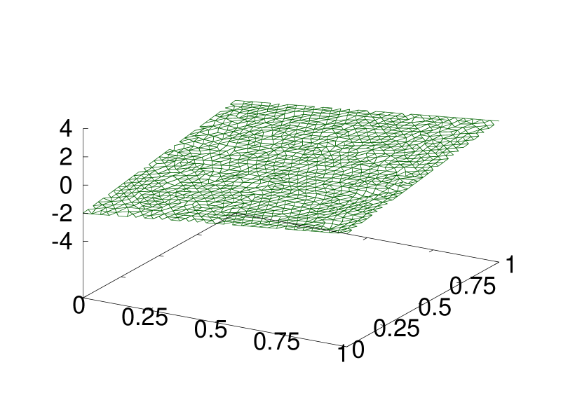
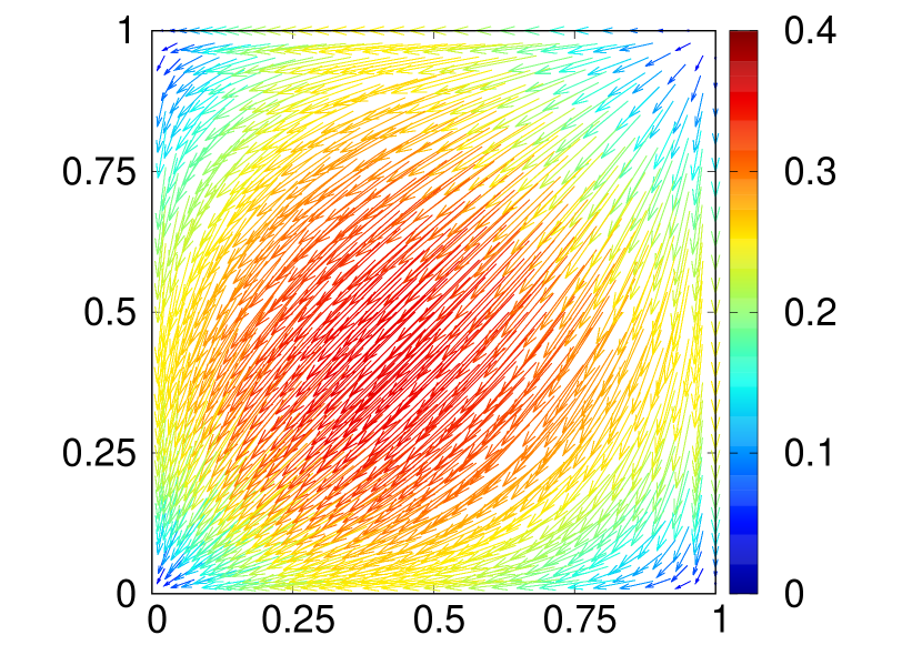
Figure 2: $p_{\mbox{\tiny$P\!P$}}$ (left) and $u_{\mbox{\tiny$P\!P$}}$ (right). The color scale indicates the length of $|u_{\mbox{\tiny$P\!P$}}(\xi)|$ at each node $\xi$.

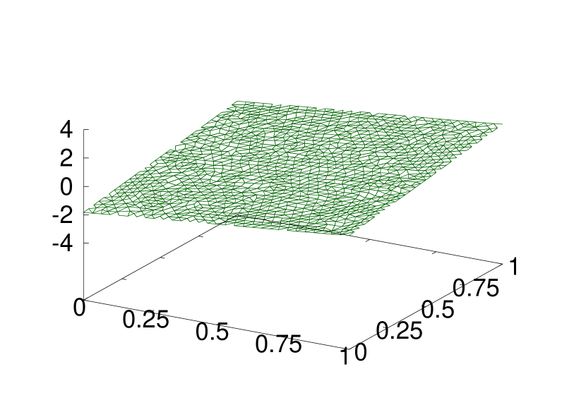
(a)

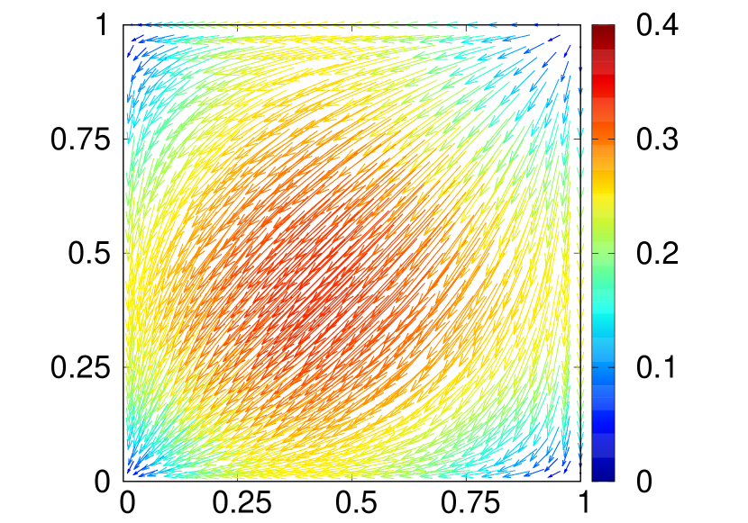
(b)

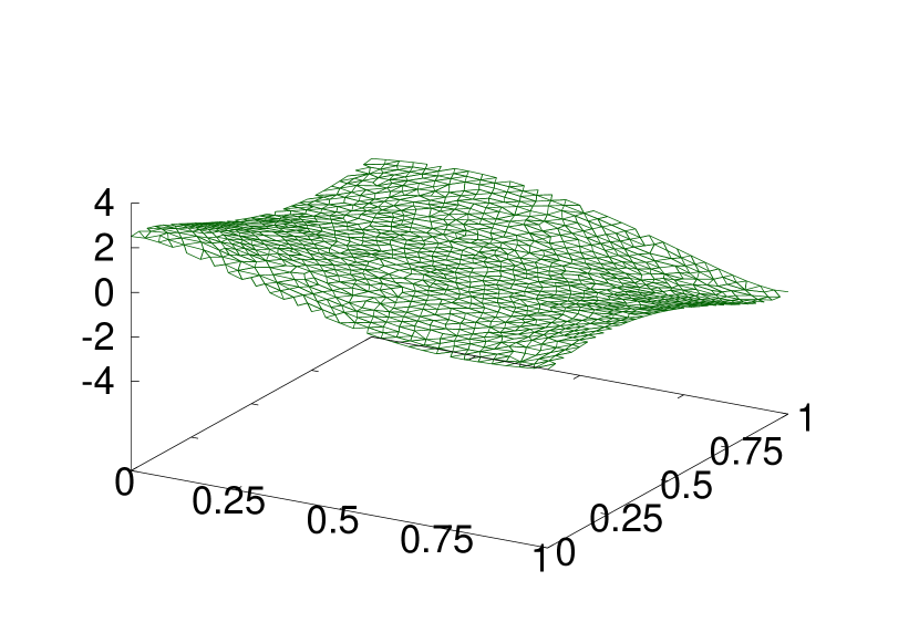
(c)

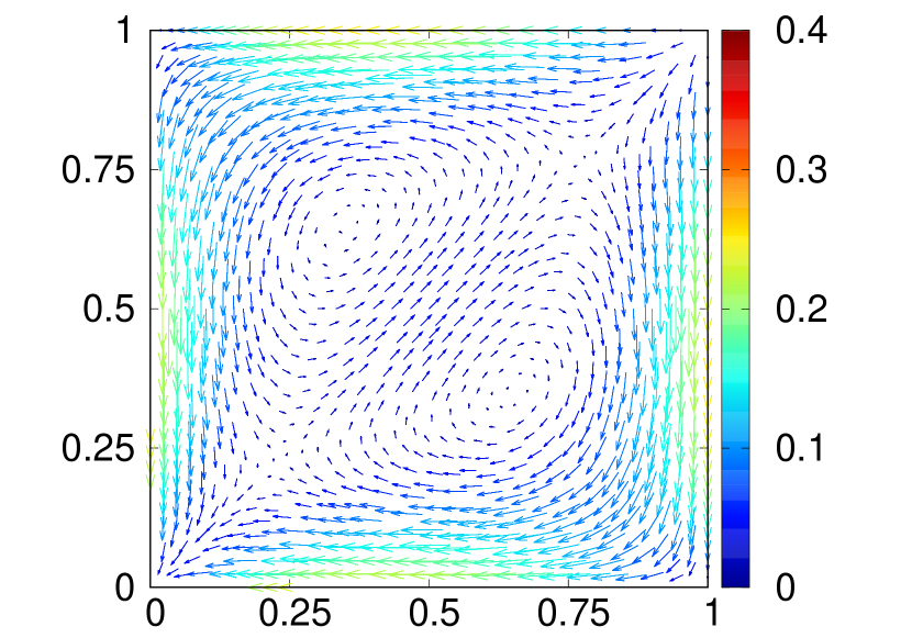
(d)

(e)

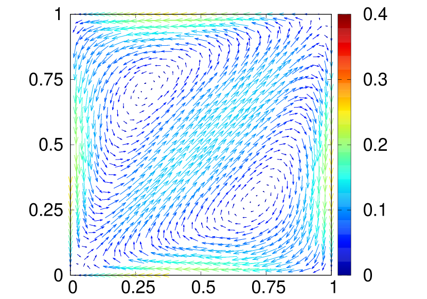
(f)

Figure 3: $p_{\varepsilon}$ (a) and $u_{\varepsilon}$ (b) with $\varepsilon=1$. $p_{\varepsilon}$ (c) and $u_{\varepsilon}$ (d) with $\varepsilon=10^{-2}$. $p_{\varepsilon}$ (e) and $u_{\varepsilon}$ (f) with $\varepsilon=10^{-4}$. The color scales indicate the length of $|u_{\varepsilon}(\xi)|$ at each node $\xi$.

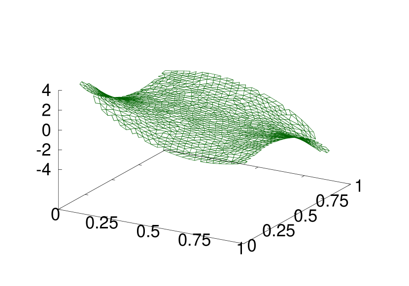
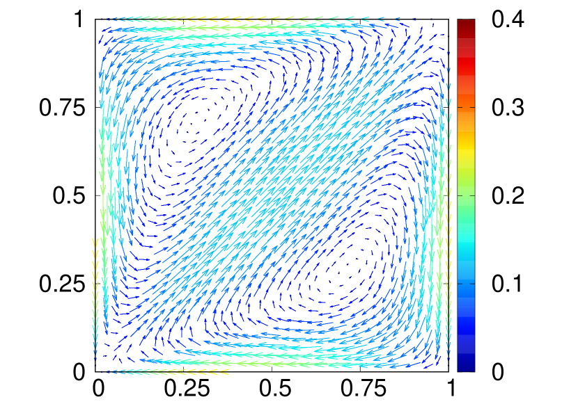
Figure 4: $p_{\mbox{\tiny$S$}}$ (left) and $u_{\mbox{\tiny$S$}}$ (right). The color scale indicates the length of $|u_{\mbox{\tiny$S$}}(\xi)|$ at each node $\xi$.

Next we compute the error estimate between the numerical solutions of (ES₁) and (PP₁). The numerical errors $\|u_{\varepsilon}-u_{\mbox{\tiny$P\!P$}}\|_{{L^{2}(\Omega)}^{n}}$, $\|\nabla(u_{\varepsilon}-u_{\mbox{\tiny$P\!P$}})\|_{{L^{2}(\Omega)}^{n\times n}}$, $\|p_{\varepsilon}-p_{\mbox{\tiny$P\!P$}}\|_{{L^{2}(\Omega)}}$ and $\|\nabla(p_{\varepsilon}-p_{\mbox{\tiny$P\!P$}})\|_{{L^{2}(\Omega)}^{n}}$ are shown in Fig. 5 and Fig. 6. Based on these values, we have fitted a constant $c$ such that $\|u_{\varepsilon}-u_{\mbox{\tiny$P\!P$}}\|_{{H^{1}(\Omega)}^{n}}\sim c/\varepsilon$ and $\|p_{\varepsilon}-p_{\mbox{\tiny$P\!P$}}\|_{{H^{1}(\Omega)}}\sim c/\varepsilon$ for $\varepsilon$ large. Fig. 5 and Fig. 6 indicate that there exists a constant $c$ such that $\|u_{\varepsilon}-u_{\mbox{\tiny$P\!P$}}\|_{{H^{1}(\Omega)}^{n}}\leq c/\varepsilon$ and $\|p_{\varepsilon}-p_{\mbox{\tiny$P\!P$}}\|_{{H^{1}(\Omega)}}\leq c/\varepsilon$, as expected from Theorem 3.2.

We also compute the error estimate between the problems (ES₁) and (S’) by numerical calculation. The numerical error estimate $\|u_{\varepsilon}-u_{\mbox{\tiny$S$}}\|_{{L^{2}(\Omega)}^{n}},~{}\|\nabla(u_{\varepsilon}-u_{\mbox{\tiny$S$}})\|_{{L^{2}(\Omega)}^{n\times n}}~{},\|p_{\varepsilon}-p_{\mbox{\tiny$S$}}\|_{{L^{2}(\Omega)}}$ and $\|\nabla(p_{\varepsilon}-p_{\mbox{\tiny$S$}})\|_{{L^{2}(\Omega)}^{n}}$ are shown in Fig. 7 and Fig. 8. Based on these values, we have fitted a constant $c$ such that $\|u_{\varepsilon}-u_{\mbox{\tiny$S$}}\|_{{H^{1}(\Omega)}^{n}}\sim c\varepsilon$ and $\|p_{\varepsilon}-p_{\mbox{\tiny$S$}}\|_{{L^{2}(\Omega)}}\sim c\varepsilon$ for $\varepsilon$ small. Fig. 7 and Fig. 8 indicate that there exists a constant $\tilde{c}$ such that $\|u_{\varepsilon}-u_{\mbox{\tiny$S$}}\|_{{H^{1}(\Omega)}^{n}}\leq\tilde{c}\sqrt{\varepsilon}$ and $\|p_{\varepsilon}-p_{\mbox{\tiny$S$}}\|_{{L^{2}(\Omega)}}\leq\tilde{c}\sqrt{\varepsilon}$, as expected from Theorem 4.4.

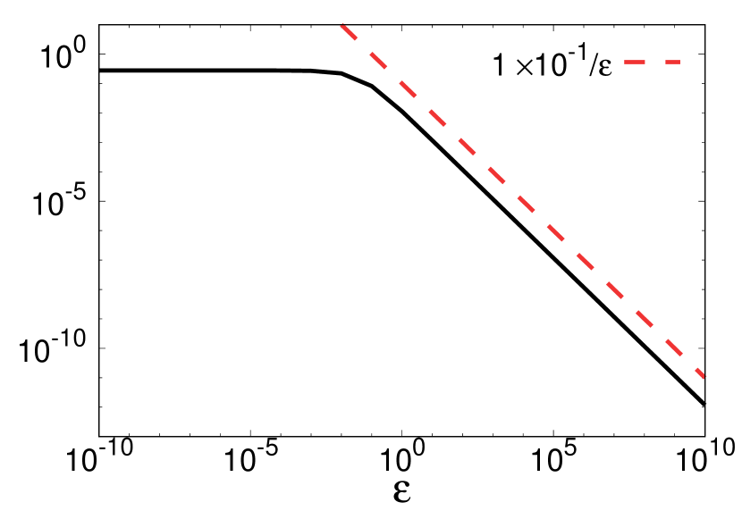
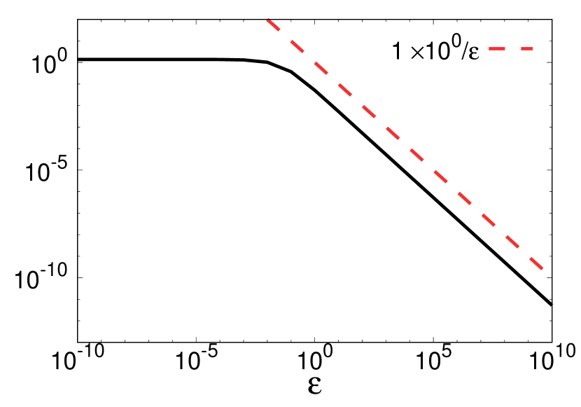
Figure 5: $\|u_{\varepsilon}-u_{\mbox{\tiny$P\!P$}}\|_{{L^{2}(\Omega)}^{n}}$ (left, solid line) and $\|\nabla(u_{\varepsilon}-u_{\mbox{\tiny$P\!P$}})\|_{{L^{2}(\Omega)}^{n\times n}}$ (right, solid line) as functions of $\varepsilon$.

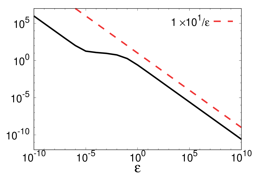
Figure 6: $\|p_{\varepsilon}-p_{\mbox{\tiny$P\!P$}}\|_{{L^{2}(\Omega)}}$ (left, solid line) and $\|\nabla(p_{\varepsilon}-p_{\mbox{\tiny$P\!P$}})\|_{{L^{2}(\Omega)}^{n}}$ (right, solid line) as functions of $\varepsilon$.

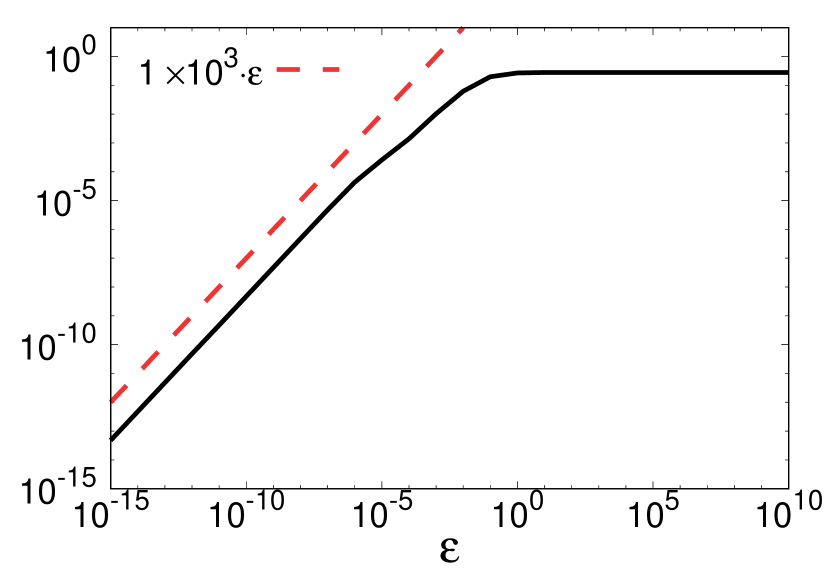
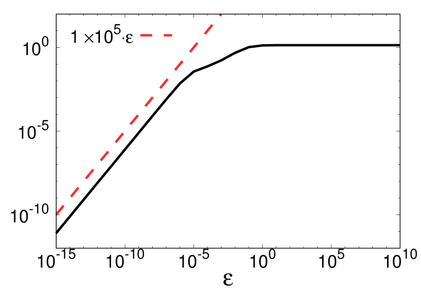
Figure 7: $\|u_{\varepsilon}-u_{\mbox{\tiny$S$}}\|_{{L^{2}(\Omega)}^{n}}$ (left, solid line) and $\|\nabla(u_{\varepsilon}-u_{\mbox{\tiny$S$}})\|_{{L^{2}(\Omega)}^{n\times n}}$ (right, solid line) as functions of $\varepsilon$.

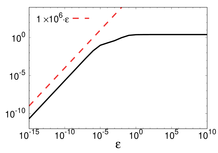
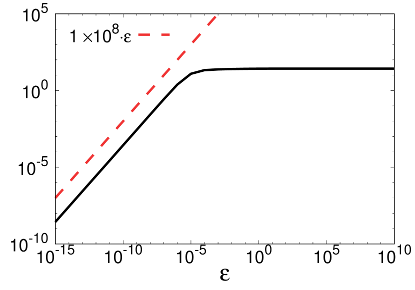
Figure 8: $\|p_{\varepsilon}-p_{\mbox{\tiny$S$}}\|_{{L^{2}(\Omega)}}$ (left, solid line) and $\|\nabla(p_{\varepsilon}-p_{\mbox{\tiny$S$}})\|_{{L^{2}(\Omega)}^{n}}$ (right, solid line) as functions of $\varepsilon$.

Appendix

Theorem 2.7, 4.2, 4.3, and Proposition 2.8 are generalizations of several theorems stated in prev . In this appendix, however, we give their proofs for the readers’ convenience. We define a continuous coercive bilinear form depending on $\varepsilon$ and prove Theorem 2.7 by the Lax–Milgram Theorem.

Proof of Theorem 2.7. We take arbitrary $u_{1}\in{H^{1}(\Omega)}^{n}$ with $\gamma_{0}u_{1}=u_{b}$. Since ${\operatorname{div}}:{H^{1}_{0}(\Omega)}^{n}\rightarrow{L^{2}(\Omega)}/{\mathbb{R}}$ is surjective (Girault, , Corollary 2.4, 2^∘), there exists $u_{2}\in{H^{1}_{0}(\Omega)}^{n}$ such that ${\operatorname{div}}u_{2}={\operatorname{div}}u_{1}$. We put

$$u_{0}:=u_{1}-u_{2},$$ (.1)

and note that $\gamma_{0}u_{0}=u_{b}$ and ${\operatorname{div}}u_{0}=0$. To simplify the notation, we set $u:=u_{\varepsilon}-u_{0}\in{H^{1}_{0}(\Omega)}^{n},p:=p_{\varepsilon}-p_{b}\in Q$, and define $f\in{H^{-1}(\Omega)}^{n}$ and $g\in Q^{*}$ by

$$\begin{array}[]{rll}\langle f,v\rangle&{\displaystyle:=\int_{\Omega}Fv-\int_{\Omega}\nabla u_{0}:\nabla v-\int_{\Omega}(\nabla p_{b})\cdot v}&\mbox{for all }v\in{H^{1}_{0}(\Omega)}^{n},\\[8.0pt] \langle g,q\rangle&{\displaystyle:=\langle G,q\rangle-\int_{\Omega}\nabla p_{b}\cdot\nabla q}&\mbox{for all }q\in Q.\end{array}$$ (.4)

Then, $(u_{\varepsilon},p_{\varepsilon})$ satisfies (ES’) if and only if $(u,p)$ satisfies

$$\left\{\begin{array}[]{ll}{\displaystyle\int_{\Omega}\nabla u:\nabla\varphi+\int_{\Omega}(\nabla p)\cdot\varphi=\langle f,\varphi\rangle}&{\rm\mbox{for all }}\varphi\in{H^{1}_{0}(\Omega)}^{n},\\[8.0pt] {\displaystyle\varepsilon\int_{\Omega}\nabla p\cdot\nabla\psi+\int_{\Omega}({\operatorname{div}}u)\psi=\varepsilon\langle g,\psi\rangle}&{\rm\mbox{for all }}\psi\in Q.\end{array}\right.$$ (.7)

Adding the equations in (.7), we get

$$\left(\left(\begin{array}[]{c}u\\ p\end{array}\right),\left(\begin{array}[]{c}\varphi\\ \psi\end{array}\right)\right)_{\varepsilon}:=\int_{\Omega}\nabla u:\nabla\varphi+\varepsilon\int_{\Omega}\nabla p\cdot\nabla\psi+\int_{\Omega}(\nabla p)\cdot\varphi+\int_{\Omega}({\operatorname{div}}u)\psi=\langle f,\varphi\rangle+\varepsilon\langle g,\psi\rangle.$$

We check that $(\cdot,\cdot)_{\varepsilon}$ is a continuous coercive bilinear form on ${H^{1}_{0}(\Omega)}^{n}\times Q$. The bilinearity and continuity of $(\cdot,\cdot)_{\varepsilon}$ are obvious. The coercivity of $(\cdot,\cdot)_{\varepsilon}$ is obtained in the following way. Take $(v,q)^{T}\in{H^{1}_{0}(\Omega)}^{n}\times Q$. We have the following sequence of inequalities:

$$\begin{array}[]{rl}\left(\left(\begin{array}[]{c}v\\ q\end{array}\right),\left(\begin{array}[]{c}v\\ q\end{array}\right)\right)_{\varepsilon}=&{\displaystyle\int_{\Omega}\nabla v:\nabla v+\varepsilon\int_{\Omega}\nabla q\cdot\nabla q+\int_{\Omega}v\cdot\nabla q+\int_{\Omega}({\operatorname{div}}v)q}\\[8.0pt] =&\|\nabla v\|^{2}_{{L^{2}(\Omega)}}+\varepsilon\|\nabla q\|^{2}_{{L^{2}(\Omega)}}\\[8.0pt] \geq&{\displaystyle{\rm min}\{1,\varepsilon\}\left(\|\nabla v\|^{2}_{{L^{2}(\Omega)}}+\|\nabla q\|^{2}_{{L^{2}(\Omega)}}\right)}\\[8.0pt] \geq&{\displaystyle c~{}{\rm min}\{1,\varepsilon\}\left(\|v\|^{2}_{{H^{1}(\Omega)}^{n}}+\|q\|^{2}_{{H^{1}(\Omega)}}\right)}.\end{array}$$

Summarizing, $(\cdot,\cdot)_{\varepsilon}$ is a continuous coercive bilinear form and ${H^{1}_{0}(\Omega)}^{n}\times Q$ is a Hilbert space. Therefore, the conclusion of Theorem 2.7 follows from the Lax–Milgram Theorem. ∎

Let $(u_{\mbox{\tiny$S$}},p_{\mbox{\tiny$S$}}),(u_{\mbox{\tiny$P\!P$}},p_{\mbox{\tiny$P\!P$}})$ and $(u_{\varepsilon},p_{\varepsilon})$ be the solutions of (S’), (PP’) and (ES’), respectively, as guaranteed by Theorem 2.5, 2.6 and 2.7. We show that the subtract $p_{\mbox{\tiny$S$}}-p_{\mbox{\tiny$P\!P$}}$ satisfies

$$\Delta(p_{\mbox{\tiny$S$}}-p_{\mbox{\tiny$P\!P$}})=0$$

in distributions sense. The weak harmonicity is the key ingredient to proving Proposition 2.8.

Proof of Proposition 2.8. First, we prove that there exists a constant $c>0$ independent of $\varepsilon$ such that $\|u_{\mbox{\tiny$S$}}-u_{\mbox{\tiny$P\!P$}}\|_{{H^{1}(\Omega)}^{n}}\leq c\|\gamma_{0}p_{\mbox{\tiny$S$}}-\gamma_{0}p_{\mbox{\tiny$P\!P$}}\|_{H^{1/2}(\Gamma)},$ and if $\gamma_{0}(p_{\mbox{\tiny$S$}}-p_{\mbox{\tiny$P\!P$}})=0$, then $p_{\mbox{\tiny$P\!P$}}=p_{\mbox{\tiny$S$}}$. Taking the divergence of the first equation of (S’), we obtain

$${\operatorname{div}}F={\operatorname{div}}(-\Delta u_{\mbox{\tiny$S$}}+\nabla p_{\mbox{\tiny$S$}})=-\Delta({\operatorname{div}}u_{\mbox{\tiny$S$}})+\Delta p_{\mbox{\tiny$S$}}=\Delta p_{\mbox{\tiny$S$}}.$$

in distributions sense. Since $p_{\mbox{\tiny$S$}}\in{H^{1}(\Omega)}$ and $C^{\infty}_{0}(\Omega)$ is dense in ${H^{1}_{0}(\Omega)}$, it follows that

$$\int_{\Omega}\nabla p_{\mbox{\tiny$S$}}\cdot\nabla\psi=-\int_{\Omega}({\operatorname{div}}F)\psi$$

for all $\psi\in{H^{1}_{0}(\Omega)}$. Together with (S’), (PP’) and ${H^{1}_{0}(\Omega)}\subset Q$, we obtain

$$\left\{\begin{array}[]{ll}{\displaystyle\int_{\Omega}\nabla(u_{\mbox{\tiny$S$}}-u_{\mbox{\tiny$P\!P$}}):\nabla\varphi=-\int_{\Omega}(\nabla(p_{\mbox{\tiny$S$}}-p_{\mbox{\tiny$P\!P$}}))\cdot\varphi}&{\rm\mbox{for all }}\varphi\in{H^{1}_{0}(\Omega)}^{n},\\[8.0pt] {\displaystyle\int_{\Omega}\nabla(p_{\mbox{\tiny$S$}}-p_{\mbox{\tiny$P\!P$}})\cdot\nabla\psi=0}&{\rm\mbox{for all }}\psi\in{H^{1}_{0}(\Omega)}\end{array}\right.$$ (.10)

from the assumption $\langle G,\psi\rangle=\int_{\Omega}\nabla F\cdot\psi$. Putting $\varphi:=u_{\mbox{\tiny$S$}}-u_{\mbox{\tiny$P\!P$}}\in{H^{1}_{0}(\Omega)}^{n}$ in (.10), we get

$$\begin{array}[]{rl}\|\nabla(u_{\mbox{\tiny$S$}}-u_{\mbox{\tiny$P\!P$}})\|^{2}_{{L^{2}(\Omega)}^{n\times n}}&={\displaystyle-\int_{\Omega}(\nabla(p_{\mbox{\tiny$S$}}-p_{\mbox{\tiny$P\!P$}}))\cdot(u_{\mbox{\tiny$S$}}-u_{\mbox{\tiny$P\!P$}})}\\[8.0pt] &\leq\|\nabla(p_{\mbox{\tiny$S$}}-p_{\mbox{\tiny$P\!P$}})\|_{{L^{2}(\Omega)}^{n}}\|u_{\mbox{\tiny$S$}}-u_{\mbox{\tiny$P\!P$}}\|_{{L^{2}(\Omega)}^{n}}.\end{array}$$

Hence,

$$\|u_{\mbox{\tiny$S$}}-u_{\mbox{\tiny$P\!P$}}\|_{{H^{1}(\Omega)}^{n}}\leq c_{1}\|\nabla(p_{\mbox{\tiny$S$}}-p_{\mbox{\tiny$P\!P$}})\|_{{L^{2}(\Omega)}^{n}}$$ (.11)

holds. From the second equation of (.10), we obtain

$$\begin{array}[]{rl}&\|\nabla(p_{\mbox{\tiny$S$}}-p_{\mbox{\tiny$P\!P$}}-\psi)\|^{2}_{{L^{2}(\Omega)}^{n}}\\ =&{\displaystyle\|\nabla(p_{\mbox{\tiny$S$}}-p_{\mbox{\tiny$P\!P$}})\|^{2}_{{L^{2}(\Omega)}^{n}}+\|\nabla\psi\|^{2}_{{L^{2}(\Omega)}^{n}}-2\int_{\Omega}\nabla(p_{\mbox{\tiny$S$}}-p_{\mbox{\tiny$P\!P$}})\cdot\nabla\psi}\\[8.0pt] =&\|\nabla(p_{\mbox{\tiny$S$}}-p_{\mbox{\tiny$P\!P$}})\|^{2}_{{L^{2}(\Omega)}^{n}}+\|\nabla\psi\|^{2}_{{L^{2}(\Omega)}^{n}}\\ \geq&\|\nabla(p_{\mbox{\tiny$S$}}-p_{\mbox{\tiny$P\!P$}})\|^{2}_{{L^{2}(\Omega)}^{n}}\end{array}$$

for all $\psi\in{H^{1}_{0}(\Omega)}$. Thus we find

$$\|\nabla(p_{\mbox{\tiny$S$}}-p_{\mbox{\tiny$P\!P$}})\|_{{L^{2}(\Omega)}^{n}}\leq\inf_{\psi\in{H^{1}_{0}(\Omega)}^{n}}\left(\|\nabla(p_{\mbox{\tiny$S$}}-p_{\mbox{\tiny$P\!P$}}-\psi)\|_{{L^{2}(\Omega)}^{n}}\right).$$

Since $\gamma_{0}$ is surjective and the space $\mbox{Ker}(\gamma_{0})={H^{1}_{0}(\Omega)}$, ${H^{1}(\Omega)}/{H^{1}_{0}(\Omega)}$ and $H^{1/2}(\Gamma)$ are isomorphic, there exists a constant $c_{2}>0$ such that $\|q\|_{{H^{1}(\Omega)}/{H^{1}_{0}(\Omega)}}\leq c_{2}\|\gamma_{0}q\|_{H^{1/2}(\Gamma)}$ for all $q\in{H^{1}(\Omega)}$. Hence, we obtain

$$\begin{array}[]{rl}\|\nabla(p_{\mbox{\tiny$S$}}-p_{\mbox{\tiny$P\!P$}})\|_{{L^{2}(\Omega)}^{n}}&\leq{\displaystyle\inf_{\psi\in{H^{1}_{0}(\Omega)}^{n}}\|\nabla(p_{\mbox{\tiny$S$}}-p_{\mbox{\tiny$P\!P$}}-\psi)\|_{{L^{2}(\Omega)}^{n}}}\\[8.0pt] &\leq{\displaystyle\inf_{\psi\in{H^{1}_{0}(\Omega)}^{n}}\|p_{\mbox{\tiny$S$}}-p_{\mbox{\tiny$P\!P$}}-\psi\|_{H^{1}(\Omega)}}\\[8.0pt] &=\|p_{\mbox{\tiny$S$}}-p_{\mbox{\tiny$P\!P$}}\|_{{H^{1}(\Omega)}/{H^{1}_{0}(\Omega)}}\\ &\leq c_{2}\|\gamma_{0}p_{\mbox{\tiny$S$}}-\gamma_{0}p_{\mbox{\tiny$P\!P$}}\|_{H^{1/2}(\Gamma)}.\end{array}$$ (.16)

Together with (.11), we obtain $\|u_{\mbox{\tiny$S$}}-u_{\mbox{\tiny$P\!P$}}\|_{{H^{1}(\Omega)}^{n}}\leq c_{1}c_{2}\|\gamma_{0}p_{\mbox{\tiny$S$}}-\gamma_{0}p_{\mbox{\tiny$P\!P$}}\|_{H^{1/2}(\Gamma)}.$ Moreover, if $\gamma_{0}(p_{\mbox{\tiny$S$}}-p_{\mbox{\tiny$P\!P$}})=0$, then $p_{\mbox{\tiny$P\!P$}}=p_{\mbox{\tiny$S$}}$.

Next, we prove that there exists a constant $c>0$ independent of $\varepsilon$ such that $\|u_{\mbox{\tiny$S$}}-u_{\varepsilon}\|_{{H^{1}(\Omega)}^{n}}\leq c\|\gamma_{0}p_{\mbox{\tiny$S$}}-\gamma_{0}p_{\varepsilon}\|_{H^{1/2}(\Gamma)},$ and if $\gamma_{0}(p_{\mbox{\tiny$S$}}-p_{\mbox{\tiny$P\!P$}})=0$, then $p_{\mbox{\tiny$P\!P$}}=p_{\varepsilon}$. Let $w_{\varepsilon}:=u_{\mbox{\tiny$S$}}-u_{\varepsilon}\in{H^{1}_{0}(\Omega)}^{n}$ and $r_{\varepsilon}:=p_{\mbox{\tiny$P\!P$}}-p_{\varepsilon}\in Q$. By (S’), (PP’) and (ES’), we obtain

$$\left\{\begin{array}[]{ll}{\displaystyle\int_{\Omega}\nabla w_{\varepsilon}:\nabla\varphi+\int_{\Omega}(\nabla r_{\varepsilon})\cdot\varphi=-\int_{\Omega}(\nabla(p_{\mbox{\tiny$S$}}-p_{\mbox{\tiny$P\!P$}}))\cdot\varphi}&{\rm\mbox{for all }}\varphi\in{H^{1}_{0}(\Omega)}^{n},\\[8.0pt] {\displaystyle\varepsilon\int_{\Omega}\nabla r_{\varepsilon}\cdot\nabla\psi+\int_{\Omega}({\operatorname{div}}w_{\varepsilon})\psi=0}&{\rm\mbox{for all }}\psi\in Q.\end{array}\right.$$ (.19)

Putting $\varphi:=w_{\varepsilon}$ and $\psi:=r_{\varepsilon}$ and adding the two equations of (.19), we get

$$\|\nabla w_{\varepsilon}\|^{2}_{{L^{2}(\Omega)}^{n\times n}}+\varepsilon\|\nabla r_{\varepsilon}\|^{2}_{{L^{2}(\Omega)}^{n}}\leq\|\nabla(p_{\mbox{\tiny$S$}}-p_{\mbox{\tiny$P\!P$}})\|_{{L^{2}(\Omega)}^{n}}\|w_{\varepsilon}\|_{{L^{2}(\Omega)}^{n}}$$ (.20)

from $\int_{\Omega}(\nabla r_{\varepsilon})\cdot w_{\varepsilon}=-\int_{\Omega}({\operatorname{div}}w_{\varepsilon})r_{\varepsilon}$. Thus we find

$$\|w_{\varepsilon}\|_{{H^{1}(\Omega)}^{n}}\leq c_{3}\|\nabla(p_{\mbox{\tiny$S$}}-p_{\mbox{\tiny$P\!P$}})\|_{{L^{2}(\Omega)}^{n}}.$$

Together with (.16), we obtain

$$\|u_{\mbox{\tiny$S$}}-u_{\varepsilon}\|_{{H^{1}(\Omega)}^{n}}=\|w_{\varepsilon}\|_{{H^{1}(\Omega)}^{n}}\leq c_{2}c_{3}\|\gamma_{0}p_{\mbox{\tiny$S$}}-\gamma_{0}p_{\mbox{\tiny$P\!P$}}\|_{H^{1/2}(\Gamma)}.$$

Moreover, by (.20), we obtain

$$\varepsilon\|p_{\mbox{\tiny$P\!P$}}-p_{\varepsilon}\|^{2}_{L^{2}(\Omega)}=\varepsilon\|r_{\varepsilon}\|^{2}_{L^{2}(\Omega)}\leq c_{4}\|\nabla(p_{\mbox{\tiny$S$}}-p_{\mbox{\tiny$P\!P$}})\|_{{L^{2}(\Omega)}^{n}}\|w_{\varepsilon}\|_{{L^{2}(\Omega)}^{n}}.$$

Hence, if $\gamma_{0}(p_{\mbox{\tiny$S$}}-p_{\mbox{\tiny$P\!P$}})=0$, then $p_{\mbox{\tiny$P\!P$}}=p_{\varepsilon}$. ∎

We show that the sequence $((u_{\varepsilon},p_{\varepsilon}))_{\varepsilon>0}$ is bounded in ${H^{1}(\Omega)}^{n}\times({L^{2}(\Omega)}/{\mathbb{R}})$. By the reflexivity of ${H^{1}(\Omega)}^{n}\times({L^{2}(\Omega)}/{\mathbb{R}})$, the sequence $((u_{\varepsilon},p_{\varepsilon}))_{\varepsilon>0}$ has a subsequence converging weakly to somewhere in ${H^{1}(\Omega)}^{n}\times({L^{2}(\Omega)}/{\mathbb{R}})$. It is sufficient to check that the limit satisfies (S’). Since the solution of (S’) is unique, the sequence $((u_{\varepsilon},p_{\varepsilon}))_{\varepsilon>0}$ converges weakly.

Proof of Theorem 4.2. We take $u_{b}\in{H^{1}(\Omega)}^{n},f\in{H^{-1}(\Omega)}^{n}$ and $g\in Q^{*}$ as (.1) and (.4) in the proof of Theorem 2.7. We put $\tilde{u}_{\varepsilon}:=u_{\varepsilon}-u_{b}\in{H^{1}_{0}(\Omega)}^{n},\tilde{p}_{\varepsilon}:=p_{\varepsilon}-p_{b}\in Q$. Then we obtain

$$\left\{\begin{array}[]{ll}{\displaystyle\int_{\Omega}\nabla\tilde{u}_{\varepsilon}:\nabla\varphi+\int_{\Omega}(\nabla\tilde{p}_{\varepsilon})\cdot\varphi=\langle f,\varphi\rangle}&{\rm\mbox{for all }}\varphi\in{H^{1}_{0}(\Omega)}^{n},\\[8.0pt] {\displaystyle\varepsilon\int_{\Omega}\nabla\tilde{p}_{\varepsilon}\cdot\nabla\psi+\int_{\Omega}({\operatorname{div}}\tilde{u}_{\varepsilon})\psi=\varepsilon\langle g,\psi\rangle}&{\rm\mbox{for all }}\psi\in Q.\end{array}\right.$$ (.23)

Putting $\varphi:=\tilde{u}_{\varepsilon},\psi:=\tilde{p}_{\varepsilon}$ and adding the two equations of (.23), we get

$$\|\nabla\tilde{u}_{\varepsilon}\|^{2}_{{L^{2}(\Omega)}^{n\times n}}+\varepsilon\|\nabla\tilde{p}_{\varepsilon}\|^{2}_{{L^{2}(\Omega)}^{n}}\leq\|f\|_{{H^{-1}(\Omega)}^{n}}\|\nabla\tilde{u}_{\varepsilon}\|_{{L^{2}(\Omega)}^{n\times n}}+\varepsilon\|g\|_{Q^{*}}\|\nabla\tilde{p}_{\varepsilon}\|_{{L^{2}(\Omega)}^{n}}$$

since $\int_{\Omega}(\nabla\tilde{p}_{\varepsilon})\cdot\tilde{u}_{\varepsilon}=-\int_{\Omega}({\operatorname{div}}\tilde{u}_{\varepsilon})\tilde{p}_{\varepsilon}$. Hence, $(\|\tilde{u}_{\varepsilon}\|_{{H^{1}(\Omega)}^{n}})_{0<\varepsilon<1}$ and $(\|\sqrt{\varepsilon}\tilde{p}_{\varepsilon}\|_{H^{1}(\Omega)})_{0<\varepsilon<1}$ are bounded. Moreover, by Lemma 4.1, we obtain

$$\|\tilde{p}_{\varepsilon}\|_{{L^{2}(\Omega)}/{\mathbb{R}}}\leq{c}(\|\nabla\tilde{u}_{\varepsilon}\|_{{L^{2}(\Omega)}^{n\times n}}+\|f\|_{{H^{-1}(\Omega)}^{n}}),$$

i.e., $(\|\tilde{p}_{\varepsilon}\|_{{L^{2}(\Omega)}/{\mathbb{R}}})_{0<\varepsilon<1}$ is bounded. By Theorem 3.2, $(\|u_{\varepsilon}\|_{{H^{1}(\Omega)}^{n}})_{\varepsilon\geq 1}$ and $(\|\tilde{p}_{\varepsilon}\|_{{L^{2}(\Omega)}/{\mathbb{R}}})_{\varepsilon\geq 1}$ are bounded, and thus $(\|u_{\varepsilon}\|_{{H^{1}(\Omega)}^{n}})_{\varepsilon>0}$ and $(\|\tilde{p}_{\varepsilon}\|_{{L^{2}(\Omega)}/{\mathbb{R}}})_{\varepsilon>0}$ are bounded.

Since ${H^{1}(\Omega)}^{n}\times({L^{2}(\Omega)}/{\mathbb{R}})$ is reflexive and $(\tilde{u}_{\varepsilon},[\tilde{p}_{\varepsilon}])_{0<\varepsilon<1}$ is bounded in ${H^{1}(\Omega)}^{n}\times({L^{2}(\Omega)}/{\mathbb{R}})$, there exist $(u,p)\in{H^{1}(\Omega)}^{n}\times({L^{2}(\Omega)}/{\mathbb{R}})$ and a subsequence of pairs $(\tilde{u}_{\varepsilon_{k}},\tilde{p}_{\varepsilon_{k}})_{k\in{\mathbb{N}}}\subset{H^{1}_{0}(\Omega)}^{n}\times Q$ such that

$$\tilde{u}_{\varepsilon_{k}}\rightharpoonup u~{}{\rm weakly~{}\mbox{in }}{H^{1}(\Omega)}^{n},~{}[\tilde{p}_{\varepsilon_{k}}]\rightharpoonup p~{}{\rm weakly~{}\mbox{in }}{L^{2}(\Omega)}/{\mathbb{R}}\quad{\rm as~{}}k\rightarrow\infty.$$

Hence, from (.23) with $\varepsilon:=\varepsilon_{k}$, taking $k\rightarrow\infty$, we obtain

$$\left\{\begin{array}[]{ll}{\displaystyle\int_{\Omega}\nabla u:\nabla\varphi+\langle\nabla p,\varphi\rangle=\langle f,\varphi\rangle}&{\rm\mbox{for all }}\varphi\in{H^{1}_{0}(\Omega)}^{n}\\[8.0pt] {\displaystyle\int_{\Omega}({\operatorname{div}}u)\psi=0}&{\rm\mbox{for all }}\psi\in Q,\end{array}\right.$$ (.26)

where we have used that

$$|\varepsilon_{k}\int_{\Omega}\nabla\tilde{p}_{\varepsilon_{k}}\cdot\nabla\psi|\leq\sqrt{\varepsilon_{k}}\|\sqrt{\varepsilon}\tilde{p}_{\varepsilon}\|_{H^{1}(\Omega)}\|\psi\|_{H^{1}(\Omega)}\rightarrow 0,$$

$$\int_{\Omega}\nabla\tilde{p}_{\varepsilon_{k}}\cdot\varphi=-\int_{\Omega}[\tilde{p}_{\varepsilon_{k}}]{\operatorname{div}}\varphi\rightarrow-\int_{\Omega}p{\operatorname{div}}\varphi=\langle\nabla p,\varphi\rangle$$

as $k\rightarrow\infty$. By (.4), the first equation of (.26) implies that

$$\int_{\Omega}\nabla(u+u_{b}):\nabla\varphi+\langle\nabla(p+p_{b}),\varphi\rangle=\int_{\Omega}F\cdot\varphi$$

for all $\varphi\in{H^{1}_{0}(\Omega)}^{n}$. From the second equation of (.26) and $C^{\infty}_{0}(\Omega)\subset Q$, ${\operatorname{div}}(u+u_{b})=0$ follows. Hence, we obtain that $(u+u_{b},p+[p_{b}])$ satisfies (S’), i.e., $u_{\mbox{\tiny$S$}}=u+u_{b}$ and $p_{\mbox{\tiny$S$}}=p+[p_{b}]$. Then we have

$$u_{\varepsilon_{k}}-u_{\mbox{\tiny$S$}}=u_{\varepsilon_{k}}-u-u_{b}=\tilde{u}_{\varepsilon_{k}}-u_{\mbox{\tiny$S$}}\rightharpoonup 0\mbox{ weakly in }{H^{1}(\Omega)}^{n},$$

$$[p_{\varepsilon_{k}}]-p_{\mbox{\tiny$S$}}=[p_{\varepsilon_{k}}-p-p_{b}]=[\tilde{p}_{\varepsilon_{k}}]-p\rightharpoonup 0\mbox{ weakly in }{L^{2}(\Omega)}/{\mathbb{R}}$$

as $k\rightarrow\infty$. Since any arbitrarily chosen subsequence of $((u_{\varepsilon},[p_{\varepsilon}]))_{0<\varepsilon<1}$ has a subsequence which converges to $(u_{\mbox{\tiny$S$}},p_{\mbox{\tiny$S$}})$, we can conclude the proof. ∎

Using Theorem 4.2 and the Rellich-Kondrachov Theorem, it is easy to prove Theorem 4.3.

Proof of Theorem 4.3. We have from (ES’) and (S’) that

$$\left\{\begin{array}[]{ll}{\displaystyle\int_{\Omega}\nabla(u_{\varepsilon}-u_{\mbox{\tiny$S$}}):\nabla\varphi+\int_{\Omega}(\nabla(p_{\varepsilon}-p_{\mbox{\tiny$S$}}))\cdot\varphi=0}&{\rm\mbox{for all }}\varphi\in{H^{1}_{0}(\Omega)}^{n},\\[8.0pt] {\displaystyle\varepsilon\int_{\Omega}\nabla p_{\varepsilon}\cdot\nabla\psi+\int_{\Omega}({\operatorname{div}}u_{\varepsilon})\psi=\varepsilon\langle G,\psi\rangle}&{\rm\mbox{for all }}\psi\in Q.\end{array}\right.$$

Putting $\varphi:=u_{\varepsilon}-u_{\mbox{\tiny$S$}}\in{H^{1}_{0}(\Omega)}^{n}$ and $\tilde{p}_{\mbox{\tiny$S$}}:=p_{\mbox{\tiny$S$}}-p_{b}\in{H^{1}(\Omega)}$, we get

$$\begin{array}[]{rl}\|\nabla(u_{\varepsilon}-u_{\mbox{\tiny$S$}})\|^{2}_{{L^{2}(\Omega)}^{n\times n}}&={\displaystyle-\int_{\Omega}(\nabla(p_{\varepsilon}-p_{\mbox{\tiny$S$}}))\cdot(u_{\varepsilon}-u_{\mbox{\tiny$S$}})}\\[8.0pt] &={\displaystyle-\int_{\Omega}(\nabla(p_{\varepsilon}-p_{b}))\cdot(u_{\varepsilon}-u_{\mbox{\tiny$S$}})+\int_{\Omega}(\nabla(p_{\mbox{\tiny$S$}}-p_{b}))\cdot(u_{\varepsilon}-u_{\mbox{\tiny$S$}})}\\[8.0pt] &={\displaystyle\int_{\Omega}(p_{\varepsilon}-p_{b}){\operatorname{div}}(u_{\varepsilon}-u_{\mbox{\tiny$S$}})+\int_{\Omega}(\nabla\tilde{p}_{\mbox{\tiny$S$}})\cdot(u_{\varepsilon}-u_{\mbox{\tiny$S$}})}\\[8.0pt] &={\displaystyle\int_{\Omega}(p_{\varepsilon}-p_{b}){\operatorname{div}}u_{\varepsilon}+\int_{\Omega}(\nabla\tilde{p}_{\mbox{\tiny$S$}})\cdot(u_{\varepsilon}-u_{\mbox{\tiny$S$}}),}\end{array}$$

since $-\int_{\Omega}(\nabla(p_{\varepsilon}-p_{b}))\cdot(u_{\varepsilon}-u_{\mbox{\tiny$S$}})=\int_{\Omega}(p_{\varepsilon}-p_{b}){\operatorname{div}}(u_{\varepsilon}-u_{\mbox{\tiny$S$}})$ and ${\operatorname{div}}u_{\mbox{\tiny$S$}}=0$. Thus,

$$\|\nabla(u_{\varepsilon}-u_{\mbox{\tiny$S$}})\|^{2}_{{L^{2}(\Omega)}^{n\times n}}=\int_{\Omega}(p_{\varepsilon}-p_{b}){\operatorname{div}}u_{\varepsilon}+\int_{\Omega}(\nabla\tilde{p}_{\mbox{\tiny$S$}})\cdot(u_{\varepsilon}-u_{\mbox{\tiny$S$}}).$$ (.27)

Putting $\psi:=p_{\varepsilon}-p_{b}\in Q$, we have

$$\varepsilon\int_{\Omega}\nabla p_{\varepsilon}\cdot\nabla(p_{\varepsilon}-p_{b})+\int_{\Omega}({\operatorname{div}}u_{\varepsilon})(p_{\varepsilon}-p_{b})=\varepsilon\langle G,p_{\varepsilon}-p_{b}\rangle.$$

Hence,

$$\varepsilon\|\nabla(p_{\varepsilon}-p_{b})\|^{2}_{{L^{2}(\Omega)}^{n}}=-\varepsilon\int_{\Omega}\nabla(p_{\varepsilon}-p_{b})\cdot\nabla p_{b}-\int_{\Omega}(p_{\varepsilon}-p_{b}){\operatorname{div}}u_{\varepsilon}+\varepsilon\langle G,p_{\varepsilon}-p_{b}\rangle.$$ (.28)

Together with (.27) and (.28), we obtain

$$\begin{array}[]{ll}&\|\nabla(u_{\varepsilon}-u_{\mbox{\tiny$S$}})\|^{2}_{{L^{2}(\Omega)}^{n\times n}}+\varepsilon\|\nabla(p_{\varepsilon}-p_{b})\|^{2}_{{L^{2}(\Omega)}^{n}}\\[8.0pt] =&{\displaystyle\int_{\Omega}\nabla\tilde{p}_{\mbox{\tiny$S$}}\cdot(u_{\varepsilon}-u_{\mbox{\tiny$S$}})-\varepsilon\int_{\Omega}\nabla(p_{\varepsilon}-p_{b})\cdot\nabla p_{b}+\varepsilon\langle G,p_{\varepsilon}-p_{b}\rangle}\\[8.0pt] \leq&\|\nabla\tilde{p}_{\mbox{\tiny$S$}}\|_{{L^{2}(\Omega)}^{n}}\|u_{\varepsilon}-u_{\mbox{\tiny$S$}}\|_{{L^{2}(\Omega)}^{n}}+\varepsilon(\|\nabla p_{b}\|_{{L^{2}(\Omega)}^{n}}+\|G\|_{Q^{*}})\|\nabla(p_{\varepsilon}-p_{b})\|_{{L^{2}(\Omega)}^{n}}.\\ \end{array}$$

By Theorem 4.2 and the Rellich-Kondrachov Theorem, there exists a sequence $(\varepsilon_{k})_{k\in{\mathbb{N}}}\subset{\mathbb{R}}$ such that

$$u_{\varepsilon_{k}}\rightarrow u_{\mbox{\tiny$S$}}\mbox{ strongly in }{L^{2}(\Omega)}^{n}\mbox{ as }k\rightarrow\infty.$$

Therefore,

$$\begin{array}[]{ll}&\|\nabla(u_{\varepsilon_{k}}-u_{\mbox{\tiny$S$}})\|^{2}_{{L^{2}(\Omega)}^{n\times n}}\\ \leq&\|\nabla\tilde{p}_{\mbox{\tiny$S$}}\|_{{L^{2}(\Omega)}^{n}}\|u_{\varepsilon_{k}}-u_{\mbox{\tiny$S$}}\|_{{L^{2}(\Omega)}^{n}}+\varepsilon_{k}(\|\nabla\tilde{p}_{b}\|_{{L^{2}(\Omega)}^{n}}+\|G\|_{Q^{*}})\|\nabla(p_{\varepsilon_{k}}-p_{\mbox{\tiny$S$}})\|_{{L^{2}(\Omega)}^{n}}\\ \rightarrow&0\end{array}$$

as $k\rightarrow\infty$. This implies that

$$\|[p_{\varepsilon_{k}}]-p_{\mbox{\tiny$S$}}\|_{{L^{2}(\Omega)}/{\mathbb{R}}}=\|p_{\varepsilon_{k}}-p_{\mbox{\tiny$S$}}\|_{{L^{2}(\Omega)}/{\mathbb{R}}}\leq c\|\nabla(u_{\varepsilon_{k}}-u_{\mbox{\tiny$S$}})\|_{{L^{2}(\Omega)}^{n\times n}}\rightarrow 0\mbox{ as }k\rightarrow\infty$$

by Lemma 4.1. Since any arbitrarily chosen subsequence of $((u_{\varepsilon},[p_{\varepsilon}]))_{0<\varepsilon<1}$ has a subsequence which converges to $(u_{\mbox{\tiny$S$}},p_{\mbox{\tiny$S$}})$, we can conclude the proof. ∎

References

(1)
Amsden, A.A., Harlow, F.H.: A simplified MAC technique for incompressible
fluid flow calculations.
J. Comput. Phys. 6, 322–325 (1970)
(2)
Chan, R.K.C., Street, R.L.: A computer study of finite-amplitude water waves.
J. Comput. Phys. 6, 68–94 (1970)
(3)
Chorin, A.J.: Numerical solution of the Navier–Stokes equations.
Math. Comput. 22(104), 745–762 (1968)
(4)
Conca, C., Murat, F., Pironneau, O.: The Stokes and Navier–Stokes
equations with boundary conditions involving the pressure.
Jpn. J. Math. 20(2), 279–318 (1994)
(6)
Cummins, S.J., Rudman, M.: An SPH projection method.
J. Comput. Phys. 152, 584–607 (1999)
(7)
Douglas, J., Wang, J.: An absolutely stabilized finite element method for the
Stokes problem.
Math. Comput. 52(186), 495–508 (1989)
(8)
Duvaut, G., Lions, J.L.: Inequalities in Mechanics and Physics,
Springer-Verlag.
Berlin (1976)
(9)
Girault, V., Raviart, P.A.: Finite Element Methods for Navier–Stokes
Equations.
Springer-Verlag (1986)
(10)
Glowinski, R.: Finite element methods for incompressible viscous flow.
In: P.G. Ciarlet, J.L. Lions (eds.) Handbook of Numerical Analysis,
vol. 9, pp. 3–1176. North-Holland (2003)
(11)
Guermond, J.L., Quartapelle, L.: On stability and convergence of projection
methods based on pressure Poisson equation.
Int. J. Numer. Meth. Fluids 26, 1039–1053 (1998)
(12)
Harlow, F.H., Welch, J.E.: Numerical calculation of time-dependent viscous
incompressible flow of fluid with a free surface.
The Physics of Fluids 8, 2182–2189 (1965)
(13)
Hecht, F.: New development in FreeFem++.
J. Numer. Math. 20(3-4), 251–265 (2012)
(14)
Hughes, T., Franca, L., Balestra, M.: A new finite element formulation for
computational fluid dynamics: V. circumventing the Babuška–Brezzi
condition: A stable Petrov–Galerkin formulation of the Stokes problem
accommodating equal-order interpolations.
Comput. Methods Appl. Mech. Engrg. 59, 85–99 (1986)
(15)
Kim, J., Moin, P.: Application of a fractional-step method to incompressible
Navier–Stokes equations.
J. Comput. Phys. 59, 308–323 (1985)
(16)
Marušić, S.: On the Navier–Stokes system with pressure boundary
condition.
Ann. Univ. Ferrara 53, 319–331 (2007)
(17)
Matsui, K., Muntean, A.: Asymptotic analysis of an -Stokes
problem connecting Stokes and pressure-Poisson problems.
Adv. Math. Sci. Appl. 27, 181–191 (2018)
(18)
McKee, S., Tomé, M.F., Cuminato, J.A., Castelo, A., Ferreira, V.G.: Recent
advances in the marker and cell method.
Arch. Comput. Meth. Engng. 2, 107–142 (2004)
(19)
Nečas, J.: Direct Methods in the Theory of Elliptic Equations.
Springer (1967).
Translated in 2012 by Kufner, A. and Tronel, G.
(20)
Perot, J.B.: An analysis of the fractional step method.
J. Comput. Phys. 108, 51–58 (1993)
(21)
Temam, R.: Navier–Stokes Equations.
North Holland (1979)
(22)
Viecelli, J.A.: A computing method for incompressible flows bounded by moving
walls.
J. Comput. Phys. 8, 119–143 (1971)