Deformed Tsallis-statistics analysis of a complex nonlinear matter-field system

Abstract

We study, using information quantifiers, the dynamics generated by a special Hamiltonian that gives a detailed account of the interaction between a classical and a quantum system. The associated, very rich dynamics displays periodicity, quasi-periodicity, not-boundedness, and chaotic regimes. Chaoticity, together with complex behavior, emerge in the proximity of an unstable entirely quantum instance. Our goal is to compare the statistical description provided by Tsallis quantifiers vis a vis that obtained with Shannon’s entropy and Jensen’s complexity.

Keywords: Tsallis Entropy, q-Statistics, Complexity, Semiquantum dynamics, Bandt-Pompe’s probabilities extraction.

, ,

1 Introduction

Quantifiers derived from information theory, like entropic forms and statistical complexities (see as examples [1, 2, 3, 4]) have been seen to be very useful for understanding the dynamics connected to time series, following the work of Kolmogorov and Sinai, who transformed Shannon’s information theory into a powerful tool for the analysis of dynamical systems [5, 6]. Of course, information theory measures and probability spaces $\Omega$ are inseparably joined quantifiers. For obtaining information quantifiers (IQ) one needs first of all to determine the probability distribution $P$ that characterizes the dynamical system or time series under scrutiny. Many techniques have been proposed for the election of $P\in\Omega$. We can mention approaches based on symbolic dynamics [7], Fourier analysis [8], and the wavelet transform [9], for example. Bandt and Pompe (BP) [10, 11] proposed a symbolic formalism for finding the probability distribution (PD) $P$ associated to an arbitrary time series (see Appendix). BP’s approach relied on peculiar traits of the attractor-construction problem through causal information, that BP include in building up the PD on is looking for. A notable BP-result is significant performance-improvement with regards to the IQs one finds by using their PD-determination methodology. One just has to assume 1) stationarity and 2) that a sufficient data-amount is some available.

1.1 Deformed $q$-statistics

It is a well-known fact that physical systems that are characterized by either long-range interactions, long-term memories, or multi-fractal nature, are best described by a generalized statistical mechanics’ formalism [12] that was proposed 30 years ago: the so-called Tsallis’ or $q$-statistics. More precisely, Tsallis [13] advanced in 1988 the idea of using in a thermodynamics’ scenario an entropic form, the Harvda-Chavrat one, characterized by the entropic index $q\in\mathcal{R}$ ($q=1$ yields the orthodox Shannon measure):

$$S_{q}=\frac{1}{(q-1)}\sum_{i=1}^{N_{s}}\left[p_{i}-(p_{i})^{q}\right],$$ (1)

where $p_{i}$ are the probabilities associated with the associated $N_{s}$ different system-configurations. The entropic index (or deformation parameter) $q$ describes the deviations of Tsallis entropy from the standard Boltzmann-Gibbs-Shannon-one

$$S=-\sum_{i=1}^{N_{s}}p_{i}\ln(p_{i}).$$ (2)

It is well-known that the orthodox entropy works best in dealing with systems composed of either independent subsystems or interacting via short-range forces whose subsystems can access all the available phase space [12]. For systems exhibiting long-range correlations, memory, or fractal properties, Tsallis’ entropy becomes the most appropriate mathematical form [14, 15, 16, 17].

1.2 Our semi-quantum physics model

Now, a topic of great interest is that of the interplay between quantum and classical systems, sometimes called semiquantum physics. If quantum effects in one of the systems are small vis-a-vis those of the other, regarding it as classical not only simplifies the description but provides profound insight into the composite system’s dynamics. One may cite as illustrations the Bloch equations [18], two-level systems interacting with an electromagnetic field within a cavity, the Jaynes-Cummings semi-classical model [19, 20], collective nuclear features [21], etc.

The system studied here [22] is of interest in both Quantum Optics and Condensed Matter [19, 20, 23, 24], particularly in view of the fact that we deal with a bosonic system that admits quasi-periodic and unbounded regimes, separated by an unstable region [25]. This feature makes the interaction with a classical mode a quite attractive phenomenon. This system has already been studied using statistical tools like Shannon-entropy and the Jensen–Shannon statistical complexity [26]. The authors showed that the pertinent statistical results agree with purely dynamical ones [26].

Our model exhibits a particularly complex sub-regime, with superposition of chaos and complexity. Therein one encounters strong correlation between classical and quantum degrees of freedom [22].

1.3 Our goal

Statistical quantifiers often allow for interesting insights into the intricacies of purely dynamical issues [27]. In such a light, the purpose of the present effort is to look for broader horizons in our statistical research, than those of [26]. This is precisely why we appeal to a possible q-statistics’ contribution to the problem, by recourse to the q-Entropy (1) and the q-statistical complexity [28], that allow for considerable enlargement of our statistical arsenal.

1.4 Methodology

Our all important PDs are extracted from times series with the BP methodology, while the time series are obtained from the Poincare-sections arising from a non linear system of equations, that represents the extant dynamics.

Section 2 deals with our semi-quantum system’s dynamics. In particular, Subsect. 2.1 gives results for the isolated quantum system while Subsect. 2.2 does so for the composite system. In Sect. 3 we exhaustively analyze our q–information quantifiers while Sect. 4 displays the pertinent results. Finally, some conclusions are drawn in Sect. 5.

2 Matter–Field Hamiltonian

Focus attention upon the Hamiltonian [22]

$$H=\varepsilon_{+}(b_{+}^{\dagger}b_{+}+\frac{1}{2})+\varepsilon_{-}(b_{-}^{\dagger}b_{-}+\frac{1}{2})+(\Delta+\alpha X)\,(b_{+}b_{-}+b_{-}^{\dagger}b_{+}^{\dagger})+\frac{\omega}{2}(P_{X}^{\,\,\,2}+X^{\,2}),$$ (3)

where $b^{\dagger}_{\pm}$, $b_{\pm}$ are boson creation and annihilation operators satisfying the standard commutation relations ($[b_{\mu},b^{\dagger}_{\nu}]=\delta_{\mu\nu}$, $[b_{\mu},b_{\nu}]=[b^{\dagger}_{\mu},b^{\dagger}_{\nu}]=0$ for $\mu,\nu=\pm$), while $\varepsilon_{\pm}>0$ are the single boson energies, and $X$, $P_{X}$ represent classical coordinate and momentum quantities, with $\omega$ the associated oscillator’s frequency.

The quantum dynamical equations are the canonical ones [23, 24], that is, arbitrary operators $O$ evolve in the Heisenberg picture as

$$i\frac{dO}{dt}=-[\>H,O\>]\,.$$ (4)

The pertinent evolution equation for the mean value $\langle O\rangle\equiv{\rm Tr}\,[\rho\,O(t)]$ becomes

$$i\frac{d\langle O\rangle}{dt}=-\langle[\>H,O\>]\rangle,$$ (5)

with the average being taken with respect to a proper quantum density matrix $\rho$. Moreover, classical variables obey the classical Hamilton’s equations of motion

$$\frac{dX}{dt} = \frac{\partial\langle H\rangle}{\partial P_{X}},$$ (6a)

$$\frac{dP_{X}}{dt} = -\frac{\partial\langle H\rangle}{\partial X}.$$ (6b)

The set of equations (5) + (6) is an autonomous one of coupled, first-order ordinary differential equations (ODE), that permits a dynamical description such that no quantum rule is violated. Particularly, commutation-relations are trivially time-conserved, since the quantum evolution is the canonical one for our effective time-dependent Hamiltonian. Note that $X$ can be viewed as a time-dependent parameter of our quantal system. The initial conditions are determined by a the quantum density matrix $\rho$. Pass now to the hermitian operators $N=b_{+}^{\dagger}b_{+}+b_{-}^{\dagger}b_{-}\,,\;\delta N=b_{+}^{\dagger}b_{+}-b_{-}^{\dagger}b_{-}\,,O_{+}=b_{+}b_{-}+b_{-}^{\dagger}b_{+}^{\dagger}\,,\\ O_{-}=i(b_{+}b_{-}-b_{-}^{\dagger}b_{+}^{\dagger})\,,$ and we are able to recast our Hamiltonian (3) as

$$H=\varepsilon\,(N+1)+\gamma\,\delta N+(\Delta+\alpha X)\,O_{+}+\frac{\omega}{2}(P_{X}^{\,\,\,2}+X^{\,2}),$$ (7)

where $\varepsilon=(\varepsilon_{+}+\varepsilon_{-})/2>0$ and $\gamma=(\varepsilon_{+}-\varepsilon_{-})/2$, with $|\gamma|<\varepsilon$. From Eqs. (5)–(6) we thus encounter a closed system of equations for our set of quantum mean values plus classical variables:

$$\frac{d\langle N+1\rangle}{dt} = 2(\Delta+\alpha X)\langle O_{-}\rangle,$$ (8a)

$$\frac{d\langle O_{-}\rangle}{dt} = 2(\Delta+\alpha X)\,\langle N+1\rangle+2\varepsilon\langle O_{+}\rangle,$$ (8b)

$$\frac{d\langle O_{+}\rangle}{dt} = -2\varepsilon\langle O_{-}\rangle,$$ (8c)

$$\frac{dX}{dt} = \omega P_{X},$$ (8d)

$$\frac{dP_{X}}{dt} = -(\omega X+\alpha\langle O_{+}\rangle),$$ (8e)

where $d\langle\delta N\rangle/dt=0$.

Eqs. (8) are clearly a nonlinear ODEs set. Non-linearity has been inserted via the coupling between the two systems, governed by the parameter $\alpha$. For $\alpha=0$ the two systems become decoupled, of course, and the precedent equations become, as a consequence, those for two independent linear systems.

The expectation value $\langle O_{-}\rangle$ is regarded as a “current”, while $\langle O_{+}\rangle$ yields the mean value of the quantum component of the interaction potential. Each level population is fixed by $\langle b^{\dagger}_{\pm}b_{\pm}\rangle=(\langle N\rangle\pm\langle\delta N\rangle)/2$. The full system (8) displays moreover the Bloch-like motion-invariant

$$I=\langle N+1\rangle^{2}-4|\langle b_{+}b_{-}\rangle|^{2}=\langle N+1\rangle^{2}-\langle O_{-}\rangle^{2}-\langle O_{+}\rangle^{2},$$ (9)

that fulfills $dI/dt=0$ in both the linear ($\alpha=0$) and nonlinear ($\alpha\neq 0$) instances, as it is easily verified.

Given that $\langle\delta N\rangle$ is conserved, it makes sense to work with the effective energy $E_{\rm eff}=\langle H\rangle-\gamma\,\langle\delta N\rangle-\varepsilon$ in place of the total energy $\langle H\rangle$. The two quantities are motion-invariants. Employing $I$ together with $E_{\rm eff}$, we diminish the amount of freedom-degrees of the system (8) to just three, which enables the employment of important tools like the Poincare sections so as to investigate the system’s dynamics.

2.1 Quantum subsystem

For $\alpha=0$, the quantum systems is fully described by the quantum Hamiltonian

$$H_{q}=\varepsilon_{+}(b_{+}^{\dagger}b_{+}+\frac{1}{2})+\varepsilon_{-}(b_{-}^{\dagger}b_{-}+\frac{1}{2})+\Delta\,(b_{+}b_{-}+b_{-}^{\dagger}b_{+}^{\dagger})\,.$$ (10)

The dynamics of this system is analyzed using a method advanced in [25, 29], that allows for diagonalization of general quadratic forms, even if they lack positivity. The pertinent dynamics displays three different regimes, according to the relation $\Delta$ - $\varepsilon$ [25]. A) One has a stable regime, for $|\Delta|<\varepsilon$, with an evolution that is bounded and quasi-periodic. The system can be separated into two traditional normal modes. This regime can further be divided into three sub-regimes according to the $H-$spectrum [25]. Always, discreteness and quasi-periodicity prevail (see [25]). B) A dynamically unstable one, for $|\Delta|>\varepsilon$. The dynamics is exponentially unbounded. The system can be split up into two normal modes. However, the creation and annihilation operators for them are non-hermitian (see [25]). C) A non-separable case for $|\Delta|=\varepsilon$. Here $H$ can no longer be cast as a sum of two-independent modes [25]. We are here at the border between the stable and unstable regimes.

2.2 The composite system: results

The distinct regimes above are determined by the relation amongst $\varepsilon$, $\Delta$, and $\alpha$, no matter what the initial conditions and $\omega$’s value may be. A) For $|\alpha|\geq\varepsilon$, the dynamics is always unbounded [22]. B) For $\varepsilon>|\alpha|$, the dynamics is determined by $\varepsilon$, $\Delta$ and $\alpha$. $\varepsilon$ competes for significance with the two coupling constants ($\Delta$ and $\alpha$). As $\alpha$ decreases, the system tends to a linear scenario and the relation between $\Delta$ and $\varepsilon$ predominates. In [22] one sees illustrative Poincare sections (see Figs. 2, 3, and 6 there). For example, if $\alpha<\varepsilon$ remains fixed but the ratio $\varepsilon/\Delta$ changes, one sees that if $\varepsilon>|\Delta|$ the dynamics is periodic and becomes quasi-periodic in the vicinity of the non-diagonalizable regime $\varepsilon=|\Delta|$, exhibiting increasing nonlinear artifacts as this region is reached (Fig. 2c of [22]). If $\varepsilon<|\Delta|$ un-boundedness reigns. One detects identical behavior for distinct values of $\alpha<\varepsilon$, if we keep the same ratio $\varepsilon/\Delta$. For augmenting values of $\alpha/\Delta$. Again, evolution from periodic curves to rather complex, quasi-periodic ones is appreciated. Finally, one reaches chaos.

The most remarkable behavior is detected at the critical case $\varepsilon\simeq|\Delta|$, in the vicinity of the non-separable instance of the linear system and at the border with the unbounded region. We discover complex, quasi-periodic evolution curves. Additionally, for appropriate “small” values of $\alpha$ ($\alpha<\Delta$), chaos is seen to emerge.

3 q–Entropy and q–Statistical Complexity

We are interested in physical processes described by a PD $P=\{p_{j},j=1,\cdots,N\}$, where $N$ is the number of available states of the physical system. We consider the normalized q–Entropy ${\mathcal{H}_{q}}$ as

$${\mathcal{H}_{q}}[P]={\rm S_{q}}[P]~{}/~{}{\rm S_{q}}[P_{e}]\ ,$$ (11)

where $S_{q}$ is given by (1) and

$${\rm S_{q}}[P_{e}]={{1-N^{1-q}}\over{q-1}}\ ,$$ (12)

the entropy corresponding to the uniform distribution $P_{e}$, for $q\in(0,1)\cup(1,\infty)$. In the Shannon case, the entropy is given by Eq. (2) ($q=1$ case) and ${\rm S_{1}}[P_{e}]=\ln N$.

As a second information measure we will use the product form for the statistical complexity advanced in [3], ${\mathcal{C}}[P]~{}=~{}{\mathcal{H}}[P]\cdot{\mathcal{Q}}[P]\$, where ${\mathcal{H}}[P]$ is an entropy and ${\mathcal{Q}}[P]$ a distance between $P$ y $P_{e}$. In our case

$${\mathcal{C}_{q}}[P]~{}=~{}{\mathcal{H}_{q}}[P]\cdot{\mathcal{Q}_{q}}[P]\ ,$$ (13)

where ${\mathcal{Q}_{q}}[P]$ is called the q-disequilibrium, defined [11] via the Jensen–Tsallis divergence ${\mathcal{J}}_{{\rm S}_{q}}$ [4]

$${\mathcal{J}}_{{\rm S}_{q}}[P,Q]~{}=~{}{{1}\over{2}}~{}K_{q}\left[P,{(P+Q)\over{2}}\right]+{{1}\over{2}}~{}K_{q}\left[Q,{(P+Q)\over{2}}\right]\ ,$$ (14)

which is the symmetric form of the q–Kullback-Leiber relative entropy

$$K_{q}\left[P,Q\right]=\frac{1}{q-1}\;\;\;\sum_{i=1}^{n}p_{i}\,[(\frac{p_{i}}{q_{i}})^{q-1}-1],$$ (15)

for $q\in(0,1)\cup(1,\infty)$. In the Shannon case, we have the Kullback-Leiber relative entropy

$$K\left[P,Q\right]=\sum_{i=1}^{n}p_{i}\ln\left(\frac{p_{i}}{q_{i}}\right).$$ (16)

The square root of ${\mathcal{J}}_{{\rm S}_{q}}$ is a metric [4]. We take

$${\mathcal{Q}_{q}}[P]={\mathcal{Q}_{q}}_{0}\cdot{\mathcal{J}}_{{\rm S}_{q}}[P,P_{e}]\ ,$$ (17)

where ${\mathcal{Q}_{q}}_{0}$ is a normalization constant ($0\leq{\mathcal{Q}_{q}}\leq 1$).

$${\mathcal{Q}_{q}}_{0}=(1-q)\cdot\left\{1-\left[{{(1+N^{q})(1+N)^{(1-q)}+(N-1)}\over{2^{(2-q)}N}}\right]\right\}^{-1}\ ,$$ (18)

and

$$Q_{0}=-2\left\{\left({{N+1}\over{N}}\right)\ln(N+1)-\ln(2N)+\ln N)\right\}^{-1}\ ,$$ (19)

in the Jensen Shannon case. The maximum disequilibrium obtains when one of the components of $P$, say $p_{k}$, is unity and the remaining components vanish. The disequilibrium ${\mathcal{Q}}$ reflects on the systems’ structure, becoming different from zero only if there exist privileged states among the available ones.

Note that ${\mathcal{C}_{q}}$ is not a trivial function of the entropy. It depends on two different probabilities distributions, namely, i) one associated to the system under analysis, $P$, and ii) the uniform distribution $P_{e}$. Moreover, it is known that for a given ${\mathcal{H}_{q}}$ value, a range of possible SC values can be gotten, from a minimum one ${\mathcal{C}_{q}}_{min}$ up to a maximum value ${\mathcal{C}_{q}}_{max}$. ${\mathcal{C}_{q}}$ provides totally original information. A general method to find the bounds ${\mathcal{C}_{q}}_{min}$ and ${\mathcal{C}_{q}}_{max}$ associated to the generalized ${\mathcal{C}}={\mathcal{H}}\cdot{\mathcal{Q}}$-quantities can be encountered in Ref. [30]. Obviously, relevant information with regards the correlation structures among the components of a physical system can be obtained from the statistical complexity quantifier. Next, we numerically analyze the system’s dynamics using the two q-quantifiers above.

4 Present results

We employ initial conditions consistent with a proper density operator. Thus, the uncertainty relationships of the quantum system are verified at all times. Precisely, the accuracy of our treatment was checked out by verifying the time-constancy of $E_{\rm eff}$ and $I$ (our dynamical invariants) up to a $10^{-10}$ precision.

Time series (TS) to build up the PDs $P$ are found using the systems’ Poincare sections (PS). Another procedure is to find the PDs using phase space’s curves, what we also did. Of course, PS’s are preferable representatives of phase space than curves in it. Our present numerical results confirm this desirability.

Our PD’s are extracted from the TS using the Bandt-Pompe technique (see the Appendix). The succession of PS’s employed in our computations are gotten via crossings with a plane, i.e., solutions of (8) with the $X(t)=0$ plane for identical values of the invariants $E_{\rm eff}$ and $I$. We also change $\varepsilon/\Delta$ and maintains constant both $\alpha/\Delta$ and $\omega/\Delta$ in the PS’s succession.

For each PS linked to a certain $\varepsilon/\Delta>1$ we work with $21$ curves, drawn by changing the initial conditions $\langle O_{-}\rangle_{0}$ and $P_{0}$ (keeping compatibility with our values for $E_{\rm eff}$ and $I$). In the unbounded zone ($\varepsilon/\Delta=1$) we require $10000$ curves. $X_{0}$, $\langle N\rangle_{0}$, and $\langle O_{+}\rangle_{0}$ are maintained constant. Further, for each PS our TS is the one associated to time-dependent values of different quantities like $\langle N+\rangle$, $\langle O_{-}\rangle$, $\langle O_{+}\rangle$, etc. The graphs depicted here are linked to the $\langle O_{+}\rangle$-case. One finds similar results for any of these quantities. We selected, per PS, $10000$ crossing-points with the plane $X(t)=0$.

A consistent Shannon (+ Jensen-Shannon) statistical description of our model, that agrees with the purely dynamic one, has been presented in [26]. The results can be observed, together with those corresponding to different values of $q$ in Figs. 1–4.

Fig. 1 displays ${\mathcal{H}_{q}}$ vs. $\varepsilon/\Delta$ for different q-values, including $q=1$. In all cases, for decreasing $\varepsilon/\Delta$ one sees that ${\mathcal{H}_{q}}$ grows (with slight oscillations), from the quasi-periodic zone ($\varepsilon/\Delta>1.2$) towards $\varepsilon/\Delta=1$, till becoming maximal at $\varepsilon/\Delta\simeq 1.05$. The dynamics teaches us that chaoticity suddenly emerges therein [22]. Afterwards, in all cases, ${\mathcal{H}_{q}}$ suddenly drops in the unbounded dynamics’ zone ($\varepsilon/\Delta\simeq 1$) till reaching an absolute minimum at ($\varepsilon/\Delta=1$). For ($\varepsilon/\Delta<1$), ${\mathcal{H}_{q}}$ is close to a minimum, almost null value. One should expect that ${\mathcal{H}_{q}}$ be smaller in this region than in the quasi-periodic (or even the non periodic) zone. The most noticeable ${\mathcal{H}_{q}}$-variations emerge in the region lying between $\varepsilon/\Delta\simeq 1.2$ and $\varepsilon/\Delta\simeq 1.05$, associated to the entropic maximum. Dynamically, this region is linked to a region in which non-linearity becomes of a more involved nature. This tales place as we attain $\varepsilon/\Delta=1.05$, near $\varepsilon/\Delta=1$, value that signals the quantum unstable scenario. Remind that here we can not find separability into quantum normal modes.

Fig. 2 displays the q–statistical complexity (SC) vs. $\varepsilon/\Delta$ for a smaller q-range. Roughly, ${\mathcal{C}_{q}}$ behaves like ${\mathcal{H}_{q}}$ for all $q$. Notice that if $\varepsilon/\Delta$ decreases, SC grows till $\varepsilon/\Delta\simeq 1.2$. Onwards, it strongly oscillates till $\varepsilon/\Delta\simeq 1.08$, attaining an absolute maximum. From this point onwards, ${\mathcal{C}_{q}}$ suddenly diminishes, reaching an absolute minimum in the unbounded zone.

Even if the minima are reached at the same $\varepsilon/\Delta$-value, the maxima of ${\mathcal{H}_{q}}$ and ${\mathcal{C}_{q}}$ are not attained in the same manner. The SC reaches its maximum sooner than the entropy in the process of approaching the unstable, quantal point. Even if the concomitant $\varepsilon/\Delta$-values do not differ too much among themselves, they are not identical.

We conclude that the descriptions via ${\mathcal{H}_{q}}$ and ${\mathcal{C}_{q}}$ can be regarded as reconfirming the $q=1$-one obtained in [26].

Fig. 3 depicts ${\mathcal{H}_{q}}$ vs. $\varepsilon/\Delta$ in the considerable ${\mathcal{H}_{q}}$–validity range $q$ $\in$ $(0,3.5)$. In this range, the entropy maximum is located in the same site $\varepsilon/\Delta\simeq 1.05$, as in the Shannon case. Instead, at $q=3.5$, the entropy no longer distinguishes between the dynamic-transition zone and the quasi-periodic one. This fact sets an upper limit to $q$. Fig. 3 is an illustration. For $q<1$, contrarily, these two zones are better distinguished. Also, we find there a stronger similitude between the curves for ${\mathcal{H}_{q}}$ and ${\mathcal{C}_{q}}$. The latter loses then significance.

Questions about the validity range (VR) for ${\mathcal{C}_{q}}$ are answered by stating that its VR is much smaller that for the entropy. Now we have $q$ $\in$ $[0.8,1.6]$. For $q>1.6$ the q-complexity absolute maximum is located in the quasi–periodic zone, not in the transition one. This result is not consistent with the dynamic results. This places an upper limit of $q=1.6$. As for a lower bound, we find $q=0.8$. This is because, for $q<0.8$, the $\varepsilon/\Delta=1.05-$value at which the q-complexity is maximal coincides with that of the entropy. We can the say that the q-complexity loses relevance. The location of the q-complexity maximum changes for $[0.8,1.6]$-q-range. The changes are not large. For $q$ $\in$ $[0.8,1.2)$ the maximum is attained at $\varepsilon/\Delta=1.08$, as in the $q=1$ case. When $q$ grows, the location grows as well, reaching $\varepsilon/\Delta=1.1$ for $q=1.6$. The optimal $\varepsilon/\Delta$-value for the ${\mathcal{C}_{q}}$-maximum cannot be obtained with our methodology. Maybe another complexity functional might be needed.

Fig. 4 depicts q-complexity curves for different $q$-values in the VR, $[0.8,1.6]$.

5 Conclusions

By recourse to Tsallis’ statistical tools we studied a non lineal Hamiltonian that describes the interaction of a quantum–matter system with a classical field. The field is represented by a single-mode electromagnetic one. The quantum system is a bosonic one that admits of both unbounded and quasi-periodic regimes. These two regimes are separated by an unstable third one [25]. The composite system is of interest in quantum optics and in condensed matter [19, 20, 23, 24].

The dynamics of the composite system is governed by a non-linear system of ordinary differential equations (ODE), given by (8). This ODE displays periodic, quasi-periodic, unbounded, chaotic, and non-linear sub-dynamics, depending on the $H$-parameters’ values. An interesting feature is that both the complex non-linear and the chaotic sub-dynamics are found lie (in the parameters’ space) in the vicinity of the unstable isolate quantum regime. Although the presence of the classical system is what enables the existence of non-linearity and chaos, one can reasonably deduce from this feature that important model’s properties emerge from the quantum system.

Our statistical tools are the q–entropy ${\mathcal{H}_{q}}$ and the q–statistical complexity ${\mathcal{C}_{q}}$, evaluated via the Bandt-Pompe symbolic analysis from time-series (TS). A specials case (q=1) is that of the Shannon entropy and Jensen-Shannon’s complexity. In turn, the TS were obtained from Poincare sections (PS) derived via our ODE system. We get the PS through intersections of the ODE’s solutions of (8) with the $X(t)=0$ plane, keeping constant the invariants $E_{\rm eff}$ and $I$. In our graphs we also keep constant i) the values of $\alpha/\Delta$ and $\omega/\Delta$ and ii) the initial conditions $X_{0}$, $\langle N\rangle_{0}$ and $\langle O_{+}\rangle_{0}$ (for all the PS-succession). One varies $\varepsilon/\Delta$.

As a first conclusion we have verified the sturdy nature of our results. The q-description (within a reasonable q-range), as seen in Figs. 1 - 2, is coherent with the Shannon’s one. Both Shannon’s entropy and ${\mathcal{H}_{q}}$ (for $0\leq q\leq 3.5)$, reach an absolute maximum at the same value of $\varepsilon/\Delta=1.05$.

As a second result we have found that our description’s validity-range is determined by ${\mathcal{C}_{q}}$. This range is $q$ $\in$ $[0.8,1.6]$ (Fig. 4), more restricted than that of the q-entropic range mentioned above (Fig. 3).

Lastly, the ${\mathcal{C}_{q}}$-maximum’s position varies between $\varepsilon/\Delta=0.8$ and $\varepsilon/\Delta=1.1$. The optimal ${\mathcal{C}_{q}}$-maximum’s position-value cannot be ascertained by recourse to the present information-tools. Maybe still more general entropic functionals, maybe of not trace-form, could become useful.

Acknowledgments. AK acknowledges support from CIC of Argentina. AP acknowledges support from CONICET of Argentina.

.1 Appendix. PD Based on Bandt and Pompe’s Methodology

To use the Bandt and Pompe [10] methodology for evaluating the probability distribution $P$ associated with the time series (dynamical system), one starts by considering partitions of the pertinent $D$-dimensional space that will hopefully “reveal” relevant details of the ordinal structure of a given one-dimensional time series $\mathcal{S}(t)=\{x_{t};t=1,\cdots,M\}$, with embedding dimension $D>1$ and time delay $\tau$. We will take here $\tau=1$ as the time delay, a parameter of the approach [10]. We are interested in “ordinal patterns”, of order $D$ [10, 31], generated by

$$(s)~{}\mapsto~{}\left(~{}x_{s-(D-1)},~{}x_{s-(D-2)},~{}\cdots,~{}x_{s-1},~{}x_{s}~{}\right),$$ (20)

which assigns to each time the $D$-dimensional vector of values at times $s,s-1,\cdots,s-(D-1)$. Clearly, the greater the $D-$value, the more information on the past is incorporated into our vectors. By “ordinal pattern” related to the time $(s)$, we mean the permutation $\pi=(r_{0},r_{1},\cdots,r_{D-1})$ of $[0,1,\cdots,D-1]$ defined by

$$x_{s-r_{D-1}}~{}\leq~{}x_{s-r_{D-2}}~{}\leq~{}\cdots~{}\leq~{}x_{s-r_{1}}~{}\leq~{}x_{s-r_{0}}.$$ (21)

In this way the vector defined by Eq. (20) is converted into a unique symbol $\hat{x}_{i}$. Thus, a permutation probability distribution $P_{x}=\{p(\hat{x}_{i}),i=1,\dots,D!\}$ is obtained from the time series $x_{i}$. The probability distribution $P$ is obtained once we fix the embedding dimension $D$ and the time delay $\tau$. The former parameter plays an important role for the evaluation of the appropriate probability distribution, since $D$ determines the number of accessible states, $D!$, and tells us about the necessary length $M$ of the time series needed in order to work with a reliable statistics. The whole enterprise works for $D!\ll M$. In particular, Bandt and Pompe [10] suggest for practical purposes to work with $3\leq D\leq 7$. For more details see [31]. We have considered in this work $D=6$, a reasonable value given in the literature for series of length $M=10000$. We have checked the results taking $D=5$, obtaining similar descriptions for the information measures considered.

                                   

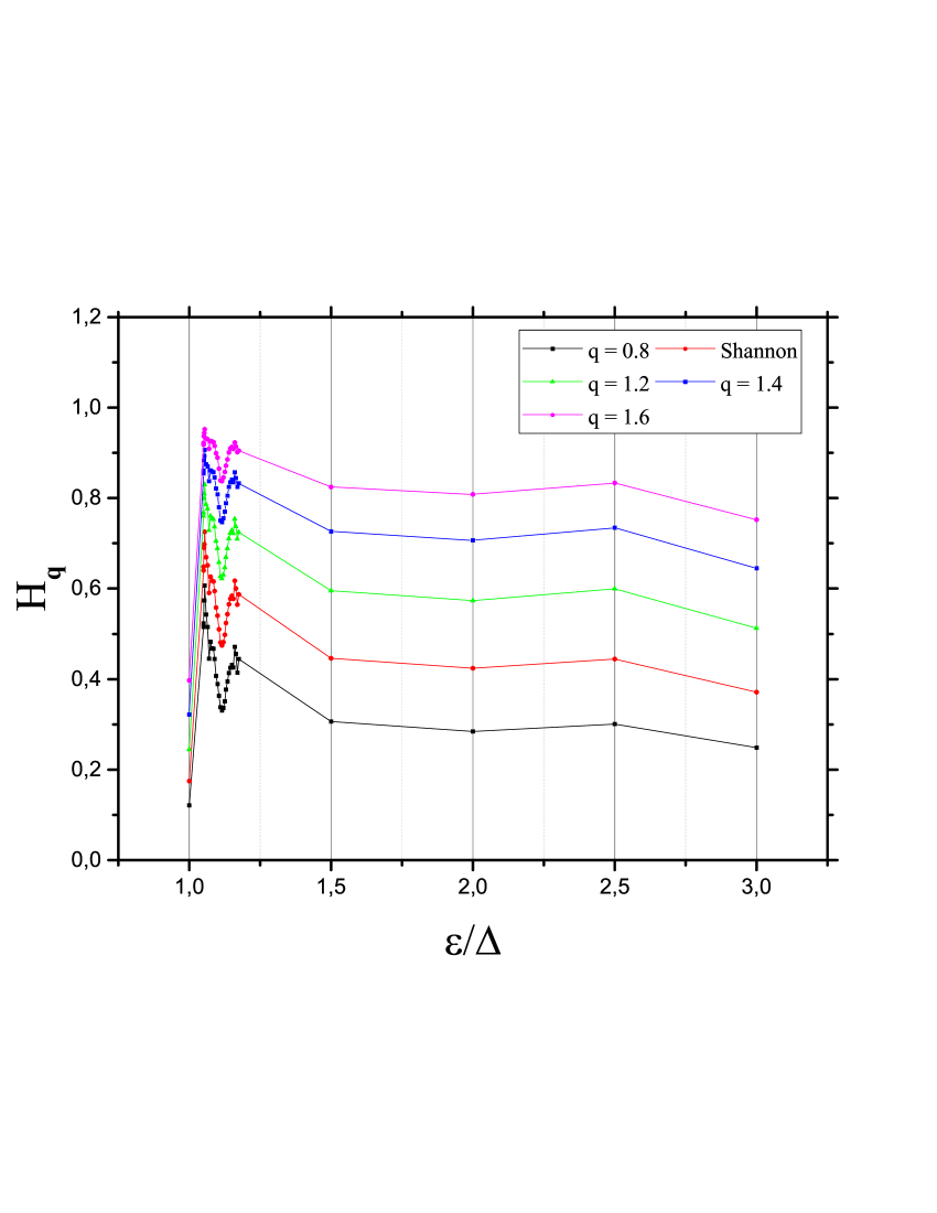
Figure 1: Entropy ${\mathcal{H}_{q}}$ vs. $\varepsilon/\Delta$ for different $q$–values, including the Shannon case. ${\mathcal{H}_{q}}$ is calculated with PDFs extracted from Poincare sections for the $X=0$ plane, corresponding to $E_{\rm eff}=4.8$ and $I=4$, with $X_{0}=1$, $\langle N\rangle_{0}=1$ and $\langle O_{+}\rangle_{0}=0$. We set $\omega/\Delta=1$ and $\alpha/\Delta=0.015$ while the ratios $\varepsilon/\Delta$ change. In all the curves, if $\varepsilon/\Delta$ decreases, ${\mathcal{H}_{q}}$ grows (with oscillations) from the quasi-periodic zone ($\varepsilon/\Delta>1.2$) towards $\varepsilon/\Delta=1$. It becomes maximal at $\varepsilon/\Delta\simeq 1.05$. Chaos suddenly emerges therein. Afterwards, ${\mathcal{H}}$ suddenly drops in the unbounded dynamics’ zone ($\varepsilon/\Delta\simeq 1$) till reaching an absolute minimum at ($\varepsilon/\Delta=1$).

                                   

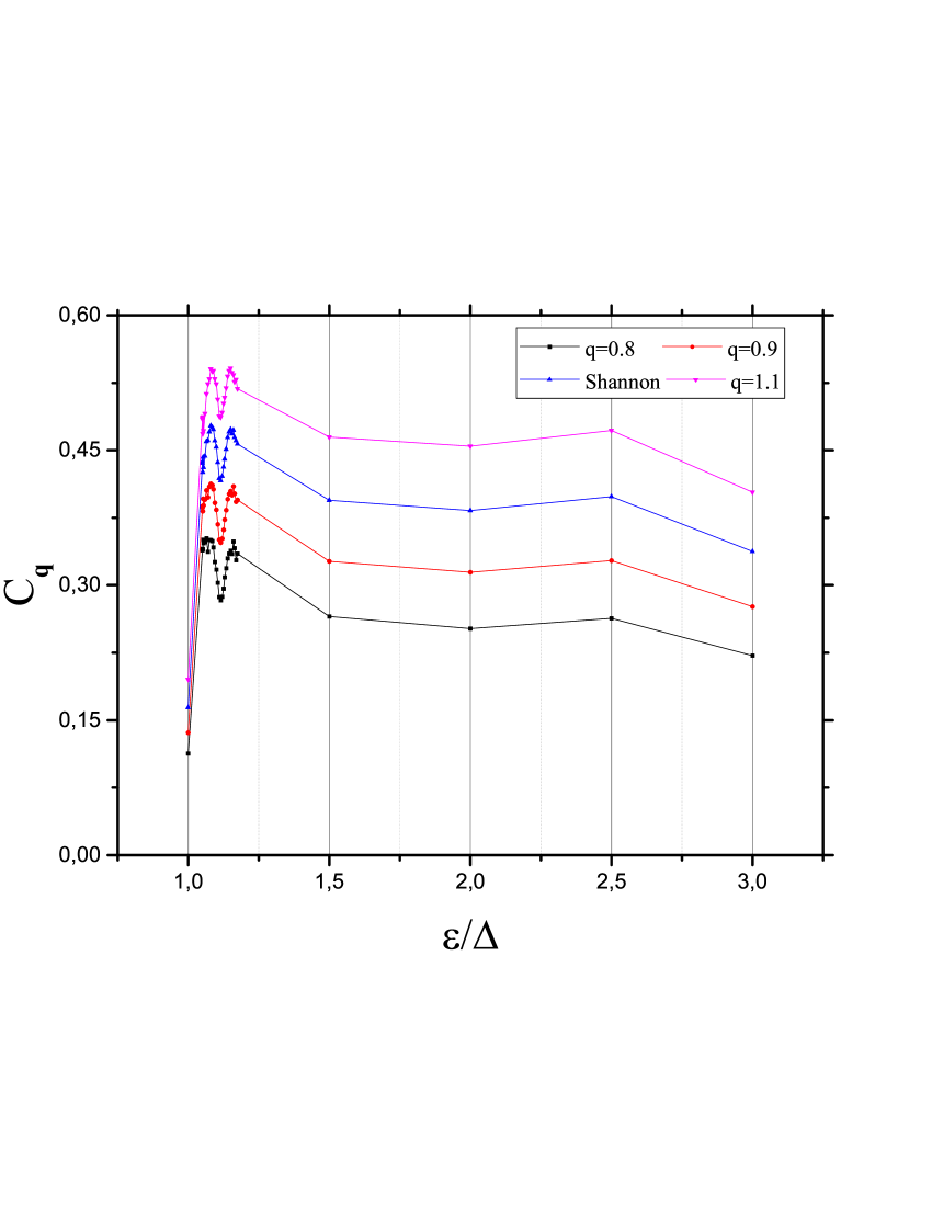
Figure 2: Statistical Complexity ${\mathcal{C}_{q}}$ vs. $\varepsilon/\Delta$, calculated as in Fig. 1. Roughly, ${\mathcal{C}_{q}}$ behaves like ${\mathcal{H}_{q}}$. For all $q$, see that if $\varepsilon/\Delta$ decreases, ${\mathcal{C}_{q}}$ grows till $\varepsilon/\Delta\simeq 1.2$. Onwards, it strongly oscillates till $\varepsilon/\Delta\simeq 1.08$, reaching an absolute maximum. Herefrom, ${\mathcal{C}_{q}}$ suddenly diminishes, reaching an absolute minimum in the unbounded zone.

                                   

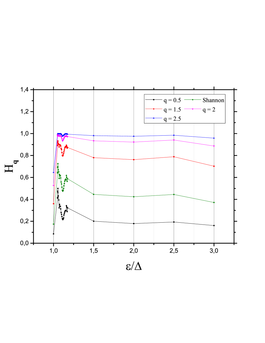
Figure 3: ${\mathcal{H}_{q}}$ vs. $\varepsilon/\Delta$, calculated as in Fig. 1, but in the ${\mathcal{H}_{q}}$–validity range $q$ $\in$ $(0,3.5)$. In this range, the entropy maximum is located at the same value of $\varepsilon/\Delta\simeq 1.05$, as in the Shannon case.

                                   

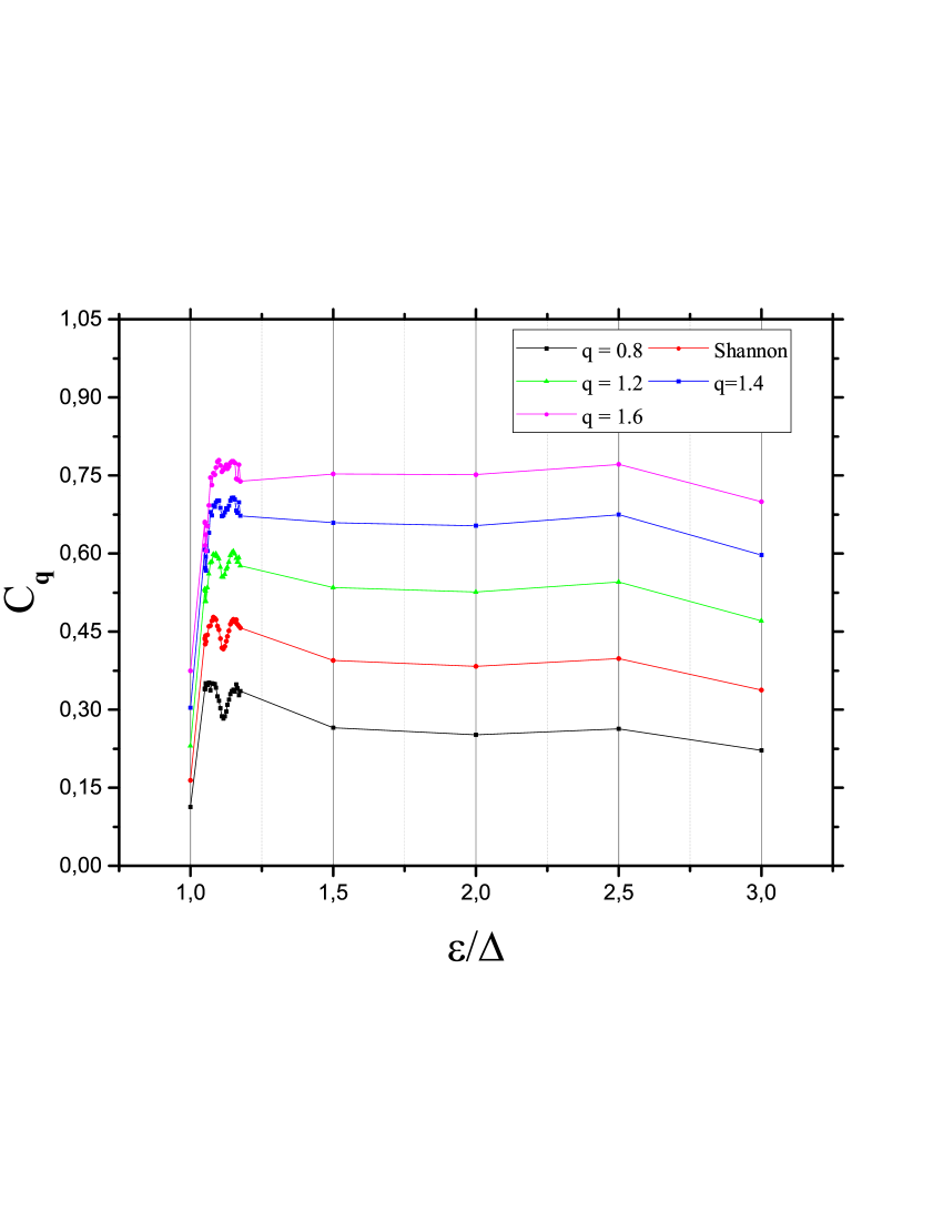
Figure 4: We plot ${\mathcal{C}_{q}}$ vs. $\varepsilon/\Delta$, as in Fig. 2, but for different $q$-values in the ${\mathcal{C}_{q}}$–validity range, $[0.8,1.6]$. The location of the q-complexity maximum changes in this range, but the changes are not significant.

References

- [1] C.E. Shannon, Bell Syst Technol Journal 27 (1948), 379; 623.
- [2] J.S. Shiner, M. Davison, P.T. Landsberg, Phys. Rev. E 59 (1999) 1459.
- [3] R. López-Ruiz, H.L. Mancini, X. Calbet, Phys. Lett. A 209 (1995) 321.
- [4] P.W. Lamberti, M.T. Martin, A. Plastino, O.A. Rosso, Physica A 334 (2004) 119.
- [5] A.N. Kolmogorov, Dokl Akad Nauk SSSR, 199 (1958) 861.
- [6] Y.G. Sinai, Dokl. Akad. Nauk SSSR, 124 (1959) 768.
- [7] K. Mischaikow, M. Mrozek, J. Reiss, A. Szymczak, Phys. Rev. Lett. 82 (1999) 1144.
- [8] G E. Powell, I C. Percival, J. Phys A: Math. Gen. 12 (1979) 2053.
- [9] O.A. Rosso, M.L. Mairal, Physica A 312, (2002) 469.
- [10] C. Bandt, B. Pompe, Phys. Rev. Lett. 88 (2002) 174102.
- [11] A.M. Kowalski, M.T. Martín, A. Plastino, O.A. Rosso, Physica D 233 (2007) 21.
- [12] R. Hanel, S. Thurner, Physica A 380 (2007) 109.
- [13] C. Tsallis, J. Stat. Phys. 52 (1988) 479.
- [14] P.A. Alemany, D.H. Zanette, Phys. Rev. E 49 (1997) R956.
- [15] C. Tsallis, Fractals 3 (1995) 541.
- [16] C. Tsallis, Phys. Rev. E 58 (1998) 1442.
- [17] M. Kalimeri, C. Papadimitriou, G. Balasis, K. Eftaxias, Physica A 387 (2008) 1161.
- [18] E. Bloch, Phys. Rev. 70 (1946) 460.
- [19] P. Milonni, M. Shih, J.R. Ackerhalt, Chaos in Laser-Matter Interactions; World Scientific Publishing Co.: Singapore, 1987.
- [20] P. Meystre, M. Sargent, Elements of Quantum Optics; Springer: NY, 1991.
- [21] P. Ring, P. Schuck, The Nuclear Many-Body Problem; Springer-Verlag: Berlin, Germany, 1980.
- [22] A.M. Kowalski, R. Rossignoli, Chaos, Solitons and Fractals 109 (2018) 140.
- [23] A.M. Kowalski, A. Plastino and A.N. Proto, Phys. Rev. E 52 (1995) 165 .
- [24] A.M. Kowalski, Physica A 458 (2016) 106.
- [25] R. Rossignoli, A.M. Kowalski, Phys. Rev. A 72 (2005) 032101.
- [26] A.M. Kowalski, A. Plastino, R. Rossignoli, Physica A (2018), doi.org/10.1016/j.physa.2018.08.159.
- [27] A. Kowalski, M.T. Martin, L. Zunino, A. Plastino, M. Casas, Entropy 12 (2010) 148.
- [28] A.M. Kowalski, A. Plastino, M. Casas, Entropy 11 (2009) 111.
- [29] R. Rossignoli, A.M. Kowalski, Phys. Rev. A 79 (2009) 062103.
- [30] M.T. Martín, A. Plastino, O.A. Rosso, Physica A 369 (2006) 439.
- [31] M. Zanin, L. Zunino, O.A. Rosso, D. Papo, Entropy 14 (2012) 1553.