A Multiversion Programming Inspired Approach to Detecting Audio Adversarial Examples^⋆

Abstract

Adversarial examples (AEs) are crafted by adding human-imperceptible perturbations to inputs such that a machine-learning based classifier incorrectly labels them. They have become a severe threat to the trustworthiness of machine learning. While AEs in the image domain have been well studied, audio AEs are less investigated. Recently, multiple techniques are proposed to generate audio AEs, which makes countermeasures against them urgent. Our experiments show that, given an audio AE, the transcription results by Automatic Speech Recognition (ASR) systems differ significantly (that is, poor transferability), as different ASR systems use different architectures, parameters, and training datasets. Based on this fact and inspired by Multiversion Programming, we propose a novel audio AE detection approach MVP-Ears, which utilizes the diverse off-the-shelf ASRs to determine whether an audio is an AE. We build the largest audio AE dataset to our knowledge, and the evaluation shows that the detection accuracy reaches 99.88%.

While transferable audio AEs are difficult to generate at this moment, they may become a reality in future. We further adapt the idea above to proactively train the detection system for coping with transferable audio AEs. Thus, the proactive detection system is one giant step ahead of attackers working on transferable AEs.

I Introduction

Automatic Speech Recognition (ASR) is a system that converts speech to text. ASR has been studied intensively for decades. Many various technologies, such as gaussian mixture models and hidden Markov models, were developed. In particular, recent advances [1] based on deep neural networks (DNNs) have improved the accuracy significantly. DNN-based speech recognition thus has become the mainstream technique in ASR systems. The industrial companies including Google, Apple and Amazon have widely adopted DNN-based ASRs for interacting with IoT devices, smart phones and cars. Gartner [2] estimates that, by 2020, 75% of American households will have at least one smart voice-enabled speaker, where DNN-based ASR plays a critical role.

Despite the great accuracy improvement, recent studies [3, 4] show that DNN is vulnerable to adversarial examples. An adversarial example (AE) $x^{\prime}$ is a mix of a host sample $x$ and a carefully crafted, human-imperceptible perturbation $\delta$ such that a DNN will assign different labels to $x^{\prime}$ and $x$. Figure 1 shows an audio AE example, which sounds as in the text shown on the left to human, but is transcribed by an ASR system into a completely different text as shown on the right.

Several techniques have been proposed to generate audio AEs. There are two state-of-the-art audio AE generation methods: (1) White-box attacks: Carlini et al. propose an optimization based method to convert an audio to an AE that transcribes to an attacker-designated phrase [5]. It is classified as white-box attacks because the target system’s detailed internal architecture and parameters are required to perform the attack. (2) Black-box attacks: Taori et al. [6] combine the genetic algorithm [7] and gradient estimation to generate AEs. This attack method does not require the knowledge of the ASR’s internal parameters, but imposes a larger perturbation (94.6% similarity on average between an AE and its original audio, compared to 99.9% in  [5]). The rapid development of audio AE generation methods makes countermeasures against audio AEs an urgent and important problem. The goal of our work is to detect audio AEs.

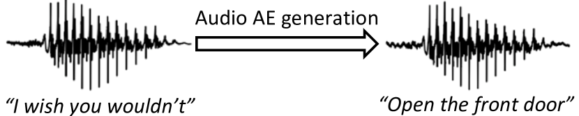
Figure 1: The generation of an audio AE.

Existing work on audio AE detection is rare and limited. Yang et al. [8] hypothesized that AEs are fragile: given an audio AE, if it is cut into two sections, which are then transcribed separately, then the transcription by splicing the two sectional results is very different from the result if the AE is transcribed as a whole. However, as admitted by the authors [8], this method cannot handle “adaptive attacks”, which may evade the detection by embedding a malicious command into one section alone. Rajaratnam et al. [9] proposed detection based on audio pre-processing methods. Yet, if an attacker knows the detection details, he can take the pre-processing effect into account when generating AEs. Such attacks have been well demonstrated for bypassing similar techniques for detecting image AEs [10]. An effective and robust audio AE detection method is missing.

Our key observation is that existing ASRs are diverse in terms of architectures, parameters and training processes. Our hypothesis is that an AE that is effective on one ASR system is likely to fail on another, which is verified by our experiments. How to generate transferable audio AEs that can fool multiple heterogeneous ASR systems is still an “open question” [5] (discussed in Section III). This inspires us to borrow the idea of multiversion programming (MVP) [11], a method in software engineering where multiple functionally equivalent programs are independently developed from the same specification, such that an exploit that compromises one program is ineffective on others. We thus propose to run multiple ASR systems in parallel, and an input is determined as an AE if the ASR systems generate very dissimilar transcription results.

Moreover, while it is unknown how to systematically generate transferable audio AEs at this moment, we predict that such techniques may be proposed in future. We thus aim to handle transferable audio AEs as well, which is a notable challenge to our system for two reasons. First, since there are no transferable audio AEs, how can our machine learning based AE detector be trained? Second, since such hypothetical transferable AEs can fool multiple ASRs, how can this idea still work?

Our first insight is that our detector essentially is not trained using AEs, but similarity scores (which are calculated based on the similarity of transcription results of different ASRs). Thus, if we assign a high similarity score between two ASRs, it simulates the effect that an AE can fool both. This way, we can conveniently generate a dataset of hypothetical AEs in the form of vectors of similarity scores. Our another insight is that, due to the complexity and diversity of ASRs, it is difficult, if not impossible, to generate audio AEs to fool all ASRs in foreseeable future. In light of this, we generate a dataset of hypothetical AEs that are rather transferable but cannot fool all ASRs. We make use of this dataset to proactively train an audio AE detection system that can keep resilient to transferable AEs, as long as there is still one ASR that cannot be fooled by the AEs. The code, datasets and models are publicly available.

We made the following contributions.

• We empirically investigate the transferability of audio AEs with multiple experiments and analyze the reasons behind the poor transferability.

• To our knowledge, we build the largest audio AE dataset, which can be reused by interested researchers.

• We propose a novel audio AE detection approach, called MVP-Ears, inspired by multiversion programming, which reaches accuracy 99.88%. The detection method dramatically reduces the flexibility of the adversary, in that audio AEs cannot succeed unless the host text is highly similar to the malicious command.

• We propose the idea of proactively training a transferable-AE detection system, such that our system is one giant step ahead of attackers who are working on generating transferable AEs.

The rest of this paper is organized as follows. We provide some background knowledge about the ASR system’s general architecture and audio AE generation in Section II. Then, we discuss the transferability of audio AEs in Section III. We describe the main idea and system architecture in Section IV and present the detailed evaluation in Section V. SectionVI gives a survey about related works. Finally, we present some discussion in Section VII and conclude in Section VIII.

II Background

II-A Automatic Speech Recognition System

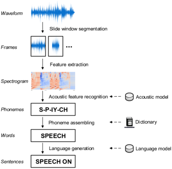
Figure 2: The process of converting an audio into a text sentence.

An Automatic speech recognition (ASR) system is used to automatically interpret human’s speech audio into texts [12]. ASR has been an active research topic since the first digit recognizer Audrey was published by Bell Laboratories in 1952. As illustrated in Figure 2, the process of converting an audio into a text sentence typically involves the following four stages: feature extraction, acoustic feature recognition, phoneme assembling, and language generation.

The input is an audio represented in the form of a waveform. (1) Feature Extraction. The input audio is first segmented into short frames, each of which is converted into feature vectors, such as MFCC feature vectors, LPC feature vectors, and PLP feature vectors. Because MFCC approximates the human auditory system’s response more closely than others, MFCC feature vector is considered as the most suitable frequency transformation format for speech data, and thus adopted by most recent ASR systems [13]. (2) Acoustic feature recognition. The extracted feature vectors are then recognized by the acoustic model as phonemes; the phoneme is the minimal unit of sounds of languages. (3) Phoneme assembling. Next, the combined phonemes are used to estimate the potential phoneme letter sequence, where the dictionary model is used to correct the word spelling of the phoneme letter sequence. (4) Language generation. At the last step, the generated words are further adjusted to the contexts and merged to the final text sentence by the language model.

The core part of an ASR system is the acoustic feature recognition stage, which outputs phonemes. A phoneme is affected by the sound in the corresponding frame and also the two adjacent frames. Different ASR models utilize different approaches to recognizing phonemes. As the features are processed with certain correlations, temporal models are well utilized, e.g.,a hybrid system of GMM and HMM (GMM-HMM). GMM-HMM is used as a statistical classifier to convert the feature vectors into phonemes, but it is limited in dealing with overlapping sound from different sources [14]. Recently, DNN-HMM [15, 16, 17] is widely used to analyze the features, and can provide better recognition performance.

However, when training GMM-HMM and DNN-HMM based ASR systems, each audio sample needs to be aligned and labeled manually at the phoneme level in order to assemble phonemes into words, which is time consuming and error-prone. To address this issue, Connectionist Temporal Classification based on Recurrent Neural Network (RNN-CTC) [18] is proposed and used for end-to-end speech recognition. CTC can directly convert the feature vectors into words without the need of generating phonemes as the intermediate result. Thus, CTC-based ASR systems outperform HMM-based ones. Deepspeech [19] is the most popular open-source implementation of a CTC-based ASR system, and is maintained regularly by Mozilla. As a result, Deepspeech is often used as the attack target model by many recent audio AE generation works.

II-B Audio Adversarial Examples

Despite the great advances and diverse applications of machine learning and deep learning [20, 21, 22], adversarial examples (AEs) [23] can be crafted to fool them. As explained by Goodfellow et al. [4], the existence of adversarial examples is due to the neural network’s linear nature. Based on this observation, they propose the Fast Gradient Sign Method (FGSM) as a simple but efficient algorithm to generate AEs.

Although a lot of successful AE attacks targeting image classification systems have been realized [24], this is not the case for the audio domain. Unlike DNN-based image classifiers where the pixels of an image are directly used as inputs of DNN, an audio needs to be first segmented into short frames with each converted into feature vectors, which are then fed into the DNN model of the ASR. Moreover, different ASRs use different lengths to segment an audio. These make the audio AE generation much more challenging. For example, by directly applying FGSM, Cisse et al. can only generate adversarial spectrogram instead of an audio AE [25].

White-box AEs. Carlini et al. overcome this limitation by adding the MFCC reconstruction layer into the backpropagation optimization of gradients and provide an end-to-end method for creating targeted audio AEs with the white-box setting [5]. It is classified as white-box attacks because the target ASR system’s detailed internal architecture and parameters are required to generate AEs.

Black-box AEs. With a black-box setting, the targeted ASR internal architecture and parameters are not known. Alzantot et al. [7] make the first effort to generate black-box AEs. They adopt the genetic algorithm to iteratively add noises into an input audio sample and discard outputs with bad performance in each generation. The iteration ends up with a black-box AE that can fool a single-word classification system (not ASR). Taori et al. [6] extend this work and combine the genetic algorithm with gradient estimation to generate black-box AEs, which can fool Deepspeech. However, the genetic algorithm-based method imposes a larger perturbation (94.6% similarity on average between a black-box AE and its original audio, compared to 99.9% between a white-box AE and its original audio). Their current AE generation only embeds up to two words in one audio.

III Transferability of AEs

There are two types of adversarial examples (AEs): non-targeted AEs and targeted AEs. A non-targeted AE is considered successful as long as it is classified as a incorrect label, while a targeted AE is successful only if it is classified as a label desired by attackers.

In the context of audio based human-computer interaction, a non-targeted AE is not very useful, as it cannot make the ASR system issue an attacker-desired command. This explains why state-of-the-art audio AE generation methods all generate targeted AEs [5, 6]. Thus, our work focuses on detection of targeted AEs, although the proposed approach is also effective in detecting non-targeted AEs (see Section V-J).

III-A Transferability in Image Domain

An intriguing property of AEs in the image domain is the existence of transferable adversarial examples. That is, an image AE crafted to mislead a specific model can also fool another different model [4, 3, 26, 27]. By exploiting this property, Papernot et al. [28] propose a reservoir-sampling based approach to generate transferable non-targeted image AEs and successfully launch black-box attacks against both image classification systems from Amazon and Google.

But a recent study [29] points out that the transferability property does not hold in some scenarios: their experiment shows a failure of AE’s transferability between a linear model and a quadratic model. For targeted image AEs, Liu et al. [30] propose an ensemble-based approach to craft AEs that can transfer to ResNet, VGG and GoogleNet models with success rates of 40%, 24%, and 11%, respectively. Thus, generating transferable image AEs is a resolved problem [31].

III-B Transferability in Audio Domain: Open Question

To the best of our knowledge, no systematic approaches have been proposed to generate transferable audio AEs. Carlini et al. [5] find that the attacking method derived from Fast Gradient Sign Method [4] in the image domain is ineffective for generating audio AEs because of a large degree of non-linearity in ASRs, and further state that the transferability of audio AEs is an open question.

A recent work CommanderSong [32] aims to generate AEs that can fool an ASR system in the presences of background noise. This work also slightly explored transferability of audio AEs (see Section 5.3 of the paper [32]). Specifically, to create AEs that can transfer from Kaldi to DeepSpeech (both Kaldi and DeepSpeech are open source ASR systems, and Kaldi is the target ASR system of CommanderSong), a two-iteration recursive AE generation method is described in CommanderSong: an AE generated by CommanderSong, embedding a malicious command $c$ and able to fool Kaldi, is used as a host sample in the second iteration of AE generation using the method [5], which targets DeepSpeech v0.1.0 and embeds the same command $c$. We followed this two-iteration recursive AE generation method to generate AEs, but our experiment results [33] showed that the generated AEs could only fool DeepSpeech but not Kaldi. That is, AEs generated using this method are not transferable.

Furthermore, we adapted the two-iteration AE generation method by concatenating the two aforementioned state-of-the-art attack methods [5] and [6] targeting DeepSpeech v0.1.0 and v0.1.1, respectively, expecting to generate AEs that can fool both DeepSpeech v0.1.0 and v0.1.1. But none of the generated AEs showed transferability [33].

Moreover, by changing the value of “--frame-subsampling-factor” from 1 to 3, which is a parameter configuration of the Kaldi model, we derived a variant of Kaldi. The AEs generated by CommanderSong did not show transferability on the variant, even given the fact that the variant was only slightly modified from the model targeted by CommanderSong. Here, we clarify that CommanderSong did not claim their AEs could transfer across the Kaldi variants.

Based on our detailed literature review and empirical study, we find that so far there are no systematic methods that can generate transferable audio AEs effective across diverse ASR systems. This is consistent with the statement by Carlini et al. [5] that transferability of audio AEs is an open question.

IV MVP-Inspired Audio AE Detection

IV-A Multi-Version Programming

Multi-version programming (MVP) was first introduced in 1977 to enhance the reliability of software and computer systems [34]. The main idea of MVP is to independently develop multiple programs based on the same specification. At runtime, multiple programs are executed concurrently and perform the same task. At each checkpoint, each program generates the result, which is to check the consistency of the execution. After that, all programs reach consensus on the execution states, and then proceed to the next stage.

The most significant benefit of MVP is relaxing the rigorous requirement of the reliability of software by providing fault tolerance from the system level. Since the multiple software programs are developed independently, the probability that they share the same flaw is very small. Especially, some implementation specific flaws usually only occur in one program. The software flaws of any program not only affect the execution flow but also cause inconsistency among comparison results. Upon detecting inconsistency, some decision algorithms are applied to determine the correct execution flow and prevent the crashing of the execution. Such a concept has already been used as an effective defense method against software flaws [35], and are widely used in development of highly reliable software, such as flight control software on modern airliners. Beside the fault tolerance, it has also been proved to be effective to detect attacks that exploit zero-day software vulnerabilities [36].

IV-B MVP-Inspired Idea

Given a system with MVP, an exploit that compromises one program probably fails on other programs. This inspires us to propose a system design that runs multiple ASRs in parallel. The intuition behind this design is that different ASRs can be regarded as ”independently developed programs” in MVP. Since they follow the same specification—that is, to covert audios into texts. Given a benign sample, they should output very similar recognition results. On the other hand, an audio AE can be regarded as an ”exploit”, and cannot fool all ASR systems as illustrated in Section III-B. Thus, by comparing the results of the multiple ASRs, we are able to determine whether an audio is an AE or not.

This idea is comparable with the ensemble approach, where multiple detection methods are combined to form a stronger one [37, 38, 39]. But they do not adopt a concise architecture like ours (e.g., [39] requires different input processing methods, while [38] needs a generalist and multiple specialists), which simply runs multiple ASRs in parallel for detection. Our work is in spirit similar to an independent work [31]. However, they differ in the following aspects: (1) That work [31] aims to detect image AEs, while our work detects audio AEs. More critically, their approach uses the softmax layer outputs as features for AE detection and attackers can thus adaptively generate the AE that leads to similar softmax outputs between models, while we use the final transcription outputs for AE detection and adaptive attacks cannot succeed unless transcriptions are similar, which is difficult as discussed in Section III-B. (2) That work only considers the bi-model design, while we consider a more general N-model design. (3) We do not stop at detecting existing audio AEs, but propose the idea for proactively training systems to detect transferable audio AEs.

IV-C Architecture

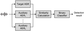
Figure 3: Architecture of the proposed detection system.

Figure 3 shows the system architecture. It consists of a target ASR, multiple auxiliary ASRs, a similarity calculation component, and a binary classifier. The target ASR is the model targeted by the adversary (e.g., the speech recognition system at a smart home), and each auxiliary ASR is a model that is different from the target ASR. The detection of AEs involves the following three steps.

• An audio is first fed into the target ASR and auxiliary ASRs. Each ASR independently and simultaneously converts the audio into a text sentence (i.e., a transcription).

• The transcriptions are then sent to the similarity calculation component, which calculates similarity scores between the transcription recognized by the target ASR and that by each auxiliary ASR.

• Finally, these similarity scores are passed into a binary classifier to determine whether the audio is adversarial.

The second step, similarity calculation, involves the following two sub-steps.

• Each transcription is converted into its phonetic-encoding representation. Phonetic encoding converts a word to the representation of its pronunciation [40]. This helps handle variations between ASRs, as they may output different words for similar sounds. The validity of using phonetic encoding is demonstrated in Section V-D.

• For each auxiliary ASR, a similarity score is calculated to measure the similarity between the transcriptions generated by the target ASR and the auxiliary ASR. We have tried different similarity measurement methods, and finally adopted the Jaro-Winkler distance method [41] due to the higher detection accuracy (see Section V-D). It outputs a score $\in[0,1]$, where 0 indicates very dissimilar and 1 similar.

IV-D Diverse ASRs

Yu and Li [42] summarized the recent progress in deep-learning based ASR acoustic models, where both recurrent neural network (RNN) and convolutional neural network (CNN) come to play as parts of deep neural networks. Standard RNN could capture sequence history in its internal states, but can only be effective for short-range sequence due to its intrinsic issue of exploding and vanishing gradients. This issue is resolved by the introduction of long short-term memory (LSTM) RNN [43], which outperforms RNNs on a variety of ASR tasks [44, 45, 46].

As to CNNs, its inherent translational invariability facilitates the exploitation of variable-length contextual information in the input speech. The first CNN model proposed for ASRs is the time delay neural network [47] that applies multiple CNN layers. Later, several studies [48, 49, 50] combine CNN and Hidden-Markov Model to create hybrid models that are more robust against vocal-tract-length variability between different speakers. However, currently, there is no single uniform structure used across all ASRs.

In addition to several opensource systems, many companies have independently developed their own proprietary ASRs, such as Google Now, Apple Siri, and Microsoft Cortana.

In our system, we use the following three ASRs, including DeepSpeech, Google Cloud Speech, and Amazon Transcribe. DeepSpeech is an end-to-end speech recognition software opensourced by Mozilla based on Baidu’s research paper [51]. DeepSpeech v0.1.0 [51] uses a five-layer neural network where the fourth layer is a RNN layer, while DeepSpeech v0.1.1 follows the same architecture and makes some improvements on the implementation. Even though these two ASR systems are very similar, our experiments (Section V-E) show that, when the two are used to build an MVP-inspired detection system, the AE detection accuracy is still very high. This means that for any target ASR system, we have potentially many candidate auxiliary ASR systems available without having to worry about the extent of (dis)similarity of the models.

Unlike DeepSpeech, the DNN behind Google Cloud Speech is a LSTM-based RNN according to the source [52]. Each memory block in Google’s LSTM network [45] is a standard LSTM memory block with an added recurrent projection layer. This design enables the model’s memory to be increased independently from the output layer and recurrent connections.

However, for Amazon Transcribe, there is no available public information about its internal details.

In short, existing ASR systems are diverse with regard to architectures, parameters and training datasets. Compared to opensource systems, proprietary ASR systems provide little information that can be exploited by attackers. Given the diversity of ASR systems (and proprietary networks), it is unclear how to propose a generic AE generation method that can simultaneously mislead all of them.

Target ASR. Our system uses DeepSpeech v0.1.0 as the target ASR. The reason is the opensource white-box AE generation method [5] targets DeepSpeech v0.1.0. Note that the generation of white-box AEs requires the knowledge of the model architecture and parameters.

Auxiliary ASRs. We use DeepSpeech v0.1.1, Google Cloud Speech, and Amazon Transcribe as the auxiliary ASRs. They are all off-the-shelf widely used ASRs.

TABLE I: Recognition results of an AE by multiple ASRs: the host transcription is “I wish you wouldn’t”, while the embedded text is “a sight for sore eyes”.

ASR	Transcribed Text
DeepSpeech v0.1.0	A sight for sore eyes
DeepSpeech v0.1.1	I wish you live
Google Cloud Speech	I wish you wouldn’t.
Amazon Transcribe	I wish you wouldn’t.

Table I shows a typical example, where the AE can only fool one ASR but fails on others. It illustrates that, given an AE, the recognition result by the target ASR differs significantly from those by the auxiliary ASRs.

IV-E Questions to Be Explored

There are still several system design questions to be answered. (Q1) How to measure the similarity of two transcriptions? (Q2) How many auxiliary ASRs work the best? More ASRs make the system more robust and resilient to attacks, but will they introduce more false positives? (Q3) Which classification algorithm works best? (Q4) Transferable audio AEs cannot be created systematically at this moment, but they may become a reality in future. How can our system be proactively trained to deal with them?

We choose to perform experiments to guide and validate the system design and answer these questions in Section V.

V Experiment-Guided System Design and the Evaluation

We finalize some system design details according to experiment results and evaluate the accuracy and robustness of the system. We first describe the experiment settings (Section V-A) and discuss the dataset used in our evaluation (Section V-B). We then investigate the feasibility of our idea (Section V-C), and examine different methods for calculating similarity scores and select the best one (Section V-D). Next, we evaluate the accuracy of our system when one auxiliary ASR is used (Section V-E) and more than one auxiliary ASR is used (Section V-F), and also evaluate the robustness of our system against unseen attack methods (Section V-G). After that, we conduct an experiment to examine whether our system can work well when facing (hypothetical) transferable AEs (Section V-H). We next evaluate the time overhead due to detection (Section V-I). Finally, we evaluate the detection effectiveness against non-targeted AEs (Section V-J).

V-A Experimental Settings

Our experiments were performed on a 64-bit Linux machine with an Intel i9-7980XE CPU @ 2.60GHz (18-core), dual NVIDIA GeForce GTX 1080 Ti, and 32GB DDR4-RAM.

As explained in Section IV-D, we use DeepSpeech v0.1.0 [53] (called DS0) as the target model. DeepSpeech v0.1.1 [53] (called DS1), Google Cloud Speech [54] (called GCS), and Amazon Transcribe [55] (called AT) are the three auxiliary ASRs. We use X$+${Y₁, …, Y_n} to denote a system using X as the target model and Y₁, …, Y_n as the auxiliary models. For example, DS0$+${DS1} means a system using DS0 as the target model and DS1 as the single auxiliary model.

TABLE II: Datasets used in our evaluation.

Dataset Name		# of Samples
Benign		2400
AE	White-box AEs	1800
	Black-box AEs	600

V-B Dataset Preparation

We consider two audio AE generation techniques: white-box based [5] and black-box based [6] methods, and build two datasets: a Benign dataset and an AE dataset, each of which contains 2400 audio samples, as shown in Table II. The audio samples of the Benign dataset are randomly selected from the dev_clean dataset of LibriSpeech [56].

The AE dataset consists of the following two parts. (1) 1800 white-box AEs, including 990 AEs provided by [5] and 810 created by us. We created the AEs following the style of [5] by using randomly selected samples from LibriSpeech as the host audios to embed the English sentences provided by [5]. (2) 600 black-box AEs constructed by applying the black-box approach [6]; each AE embeds only two words. The two-word limit is due to the current capacity of [6]. Each white-box AE takes 18 minutes on average to generate, while each black-box AE takes 90 minutes. The datasets and the transcription details are made publicly available. We have verified that all AEs can successfully fool the target model DS0.

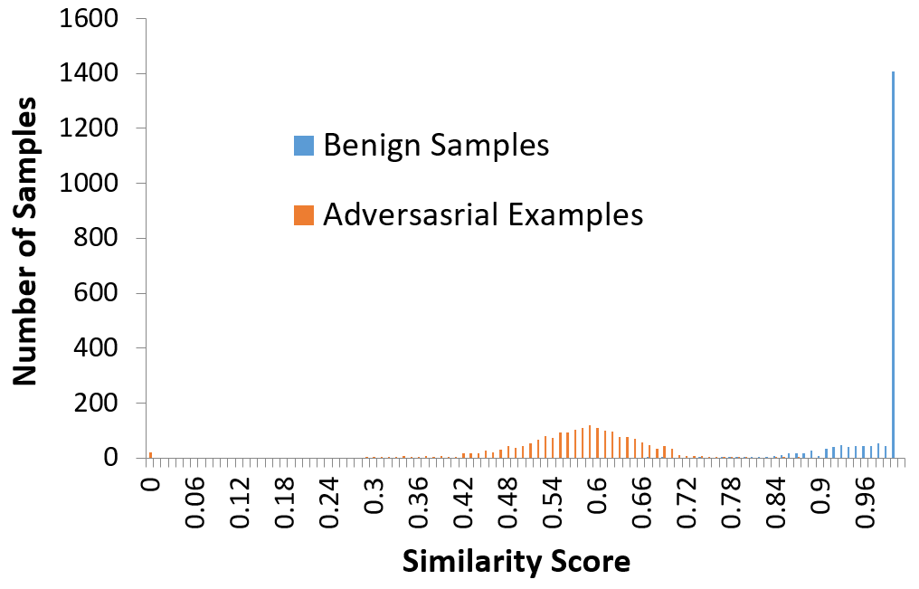
(a) DS0$+${DS1}

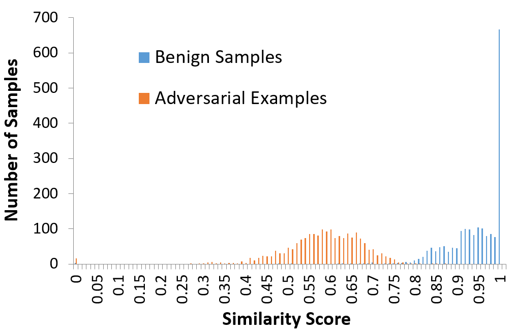
(b) DS0$+${GCS}

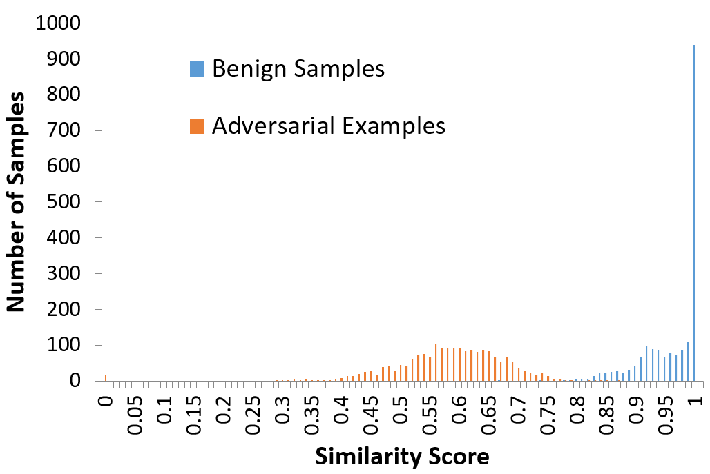
(c) DS0$+${AT}

Figure 4: Similarity score histograms of the three single-auxiliary-model systems.

V-C Feasibility Analysis

To validate the feasibility of the MVP-inspired idea, we feed all the benign samples and AEs into each of the four ASRs, and calculate the similarity scores. Given an audio (benign sample or AE), the similarity score indicates the similarity of the transcription of DS0 and that of an auxiliary ASR.

The histograms in Figure 4 confirm the feasibility of the idea: in each of the three cases, the similarity scores for AEs and those for benign samples form two almost disjoint clusters. It means that benign samples lead to relatively high similarity scores, while AEs low scores.

TABLE III: Accuracies when different similarity calculation methods are used.

Similarity Method	Performance	System
		DS0$+${DS1, GCS}	DS0$+${DS1, AT}	DS0$+${GCS, AT}	DS0$+${DS1, GCS, AT}
Cosine	Accuracy	958/960 (99.79%)	957/960 (99.69%)	952/960 (99.17%)	957/960 (99.69%)
	FPR	2/480 (0.42%)	2/480 (0.42%)	7/480 (1.46%)	2/480 (0.42%)
	FNR	0/480 (0.00%)	1/480 (0.21%)	1/480 (0.21%)	1/480 (0.21%)
Jaccard	Accuracy	957/960 (99.69%)	958/960 (99.79%)	921/960 (95.94%)	956/960 (99.58%)
	FPR	3/480 (0.63%)	2/480 (0.42%)	38/480 (7.92%)	4/480 (0.83%)
	FNR	0/480 (0.00%)	0/480 (0.00%)	1/480 (0.21%)	0/480 (0.00%)
JaroWinkler	Accuracy	958/960 (99.79%)	958/960 (99.79%)	956/960 (99.58%)	958/960 (99.79%)
	FPR	1/480 (0.21%)	1/480 (0.21%)	2/480 (0.42%)	1/480 (0.21%)
	FNR	1/480 (0.21%)	1/480 (0.21%)	2/480 (0.42%)	1/480 (0.21%)
PE_Cosine	Accuracy	958/960 (99.79%)	958/960 (99.79%)	957/960 (99.69%)	958/960 (99.79%)
	FPR	2/480 (0.42%)	2/480 (0.42%)	2/480 (0.42%)	2/480 (0.42%)
	FNR	0/480 (0.00%)	0/480 (0.00%)	1/480 (0.21%)	0/480 (0.00%)
PE_Jaccard	Accuracy	958/960 (99.79%)	958/960 (99.79%)	443/960 (99.69%)	958/960 (99.79%)
	FPR	2/480 (0.42%)	2/480 (0.42%)	3/480 (0.63%)	2/480 (0.42%)
	FNR	0/480 (0.00%)	0/480 (0.00%)	0/480 (0.00%)	0/480 (0.00%)
PE_JaroWinkler	Accuracy	958/960 (99.79%)	959/960 (99.90%)	958/960 (99.79%)	959/960 (99.90%)
	FPR	1/480 (0.21%)	0/480 (0.00%)	0/480 (0.00%)	1/480 (0.21%)
	FNR	1/480 (0.21%)	1/480 (0.21%)	2/480 (0.42%)	0/480 (0.00%)

V-D Choosing Similarity Calculation Methods

Many methods can be used to measure the similarity between two strings. Some well-known ones include Jaccard index [57], Cosine similarity, and Edit distance (e.g., JaroWinkler [41]). In addition, we propose to convert the transcription into its phonetic encoding (PE) [40]. Our hypothesis is that this may help reduce the false positives: given a benign sample, different ASRs may output different words of similar pronunciations, which can lead to higher similarity scores after phonetic encoding.

To choose the similarity measurement method and validate the hypothesis above, we consider six different combinations of similarity calculation methods, as shown in Table III. For example, PE_JaroWinkler means phonetic encoding and JaroWinkler are used as the similarity calculation method. In each case, we train a SVM based classifier using 80% of audios in the two datasets (Benign and AE), and then test the classifier using the rest 20% (that is, 4800 * 0.2 = 960 audios). Table III shows that the combination PE_JaroWinkler achieves the highest accuracies in all the four example systems. For example, when DS1, GCS, AT are used as the auxiliary ASRs, it achieves the accuracy 99.90%(, although other methods also lead to high accuracies at least 99.58%). Thus, we choose PE_JaroWinkler as the similarity calculation method.

TABLE IV: Testing results of single-auxiliary-model systems. The mean and standard deviation across the 5-fold cross validation are reported, denoted as mean/STD. FPR: false positive rate; FNR: false negative rate.

Classifier	Performance	System
		DS0$+${DS1}	DS0$+${GCS}	DS0$+${AT}
SVM	Accuracy	99.56% / 0.18%	98.92% / 0.22%	99.71% / 0.14%
	FPR	0.38% / 0.16%	1.71% / 0.40%	0.25% / 0.24%
	FNR	0.50% / 0.41%	0.46% / 0.24%	0.34% / 0.21%
KNN	Accuracy	99.36% / 0.12%	98.35% / 0.12%	99.65% / 0.16%
	FPR	0.67% / 0.27%	2.04% / 0.16%	0.25% / 0.24%
	FNR	0.63% / 0.48%	1.25% / 0.19%	0.46% / 0.24%
Random Forest	Accuracy	99.31% / 0.19%	98.04% / 0.15%	99.54% / 0.21%
	FPR	0.63% / 0.23%	2.21% / 0.39%	0.46% / 0.24%
	FNR	0.75% / 0.60%	1.71% / 0.15%	0.46% / 0.33%

V-E Effectiveness of Single-Auxiliary-Model Systems

A detection system that uses a single auxiliary ASR has the advantage of a cheap deployment. We build three such systems: DS0$+${DS1}, DS0$+${GCS}, and DS0$+${AT}. We use k-fold cross validation (k = 5) to evaluate the three systems: the datasets are divided into 5 equal subsets and, in each of the five runs, one subset is used for testing and the rest four for training. As shown in Table IV, the mean and standard deviation of the results across the 5 runs are reported.

We use three different binary classifiers, including SVM, KNN and Random Forest, and configure each classifier as follows: (1) SVM uses a 3-degree polynomial kernel; (2) KNN uses 10 neighbors to vote; and (3) Random Forest uses a seed of 200 as the starting random state.

Based on the results, we conclude that (1) all the single-auxiliary-model systems achieve high accuracies (over 98%) and low FPRs/FNRs; and (2) SVM performs slightly better than the other two classifier methods.

But it is worth mentioning that if the auxiliary ASR (like Kaldi) is not accurate in recognizing benign audios, the AE detection accuracy is bad (e.g., <80% with Kaldi).

TABLE V: 5-fold cross validation testing results (reported as mean/STD) of four multi-auxiliary-model systems.

Classifier	Performance	System
		DS0$+${DS1, GCS}	DS0$+${DS1, AT}	DS0$+${GCS, AT}	DS0$+${DS1, GCS, AT}
SVM	Accuracy	99.75% / 0.05%	99.86% / 0.08%	99.82% / 0.10%	99.88% / 0.10%
	FPR	0.29% / 0.21%	0.08% / 0.10%	0.08% / 0.10%	0.04% / 0.08%
	FNR	0.21% / 0.23%	0.21% / 0.23%	0.29% / 0.21%	0.21% / 0.23%
KNN	Accuracy	99.77% / 0.04%	99.81% / 0.08%	99.75% / 0.17%	99.86% / 0.08%
	FPR	0.25% / 0.16%	0.13% / 0.10%	0.21% / 0.23%	0.08% / 0.10%
	FNR	0.21% / 0.23%	0.25% / 0.21%	0.29% / 0.21%	0.21% / 0.23%
Random Forest	Accuracy	99.73%  0.08%	99.81% / 0.12%	99.77% / 0.08%	99.84% / 0.08%
	FPR	0.25% / 0.16%	0.13% / 0.17%	0.17% / 0.08%	0.08% / 0.10%
	FNR	0.29% / 0.28%	0.25% / 0.21%	0.29% / 0.21%	0.25% / 0.21%

TABLE VI: Impact of the number of ASRs on FPR and FNR.

# of Aux. ASRs	System	FPR	FNR
1	DS0+{DS1}	0.38%	0.50%
	DS0+{GCS}	1.71%	0.46%
	DS0+{AT}	0.25%	0.34%
2	DS0+{DS1, GCS}	0.29%	0.21%
	DS0+{DS1, AT}	0.08%	0.21%
	DS0+{GCS, AT}	0.08%	0.29%
3	DS0+{DS1, GCS, AT}	0.04%	0.21%

V-F Effectiveness of Multi-Auxiliary-Model Systems

A multi-auxiliary-model system uses more than one auxiliary model. We build four multiple-auxiliary-model systems, denoted as: DS0$+${DS1, GCS}, DS0$+${DS1, AT}, DS0$+${GCS, AT}, and DS0$+${DS1, GCS, AT}.

For a multi-auxiliary-model system with $n$ auxiliary models, given an input audio, $n$ similarity scores are calculated and form a feature vector. The feature vector is then fed into the binary classifier to predict whether the audio is an AE.

Table V shows the testing results using 5-fold cross validation. All the accuracy results are higher than 99.70%, and FPR and FNR are lower than 0.30%, regardless of the auxiliary models and binary classifiers used. The three-auxiliary-model system performs the best and reaches the accuracy 99.88%. We also observe that a system with more auxiliary models achieves better accuracy, probably because extra models provide more features in the feature vector.

Does FPR increase due to more auxiliary ASRs? To answer this intriguing question, we extract the FPR and FNR results when SVM is used as the binary classifier from Table IV and Table V and obtain Table VI, which shows that both FPRs and FNRs tend to slightly decline when more auxiliary ASRs are used. This conclusion holds when either KNN or RandomForest is used as the binary classifier.

TABLE VII: The detection results of unseen-attack AEs for three single-auxiliary-models.

System	Threshold	FPR	FNs	FNR	Defense rate
DS0$+${DS1}	0.88	4.13%	0	0.00%	100%
DS0$+${GCS}	0.82	4.75%	4	0.17%	99.83%
DS0$+${AT}	0.85	3.92%	2	0.08%	99.92%

(a) DS0$+${DS1}

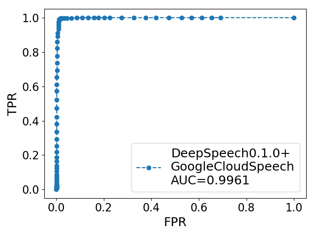
(b) DS0$+${GCS}

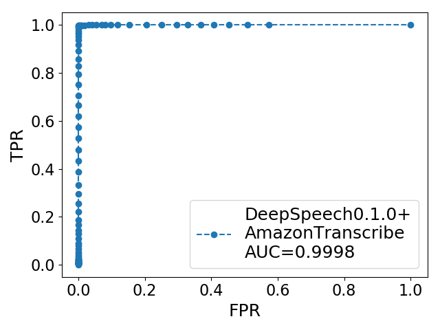
(c) DS0$+${AT}

Figure 5: The ROC curves of the three single-auxiliary-model systems.

V-G Robustness against Unseen Attack Methods

This experiment aims to examine whether a system trained on AEs generated by a particular attack method is able to detect AEs generated by other kinds of attack methods—such an AE is called an unseen-attack AE. We use the defense rate, defined as the ratio of the number of successfully detected AEs among the total number of AEs, to measure the robustness.

Single-auxiliary-model systems. We first examine all the three single-auxiliary-model systems. We train each system using only the 2400 benign samples, and test it using all the 2400 AEs (see Table II), which all can can be considered as unseen-attack AEs.

We simply use a similarity score threshold $T$ for detecting AEs: an audio that has a score lower than $T$ is detected as an AE. First, the threshold is determined by having the FPR less than 5%. The detection results are presented in Table VII. Each of the three detection systems achieves excellent defense rates $\geq$ 99.83%. Second, we vary $T$ and obtain the Receiver Operating Characteristic (ROC) curve, as shown in Figure 5. The AUC in each case is close to 1, implying high detection accuracies, which is consistent with the results of the machine learning based approaches (see Section V-E).

TABLE VIII: The detection results of unseen-attack AEs for four multiple-auxiliary-models.

System	Defense rate
	Black-box AEs	White-box AEs
DS0$+${DS1, GCS}	99.33%	100%
DS0$+${DS1, AT}	99.17%	100%
DS0$+${GCS, AT}	99.33%	99.89%
DS0$+${DS1, GCS, AT}	99.33%	100%

Multiple-auxiliary-model systems. We next examine the four multiple-auxiliary-model systems. As aforementioned, two different methods are used to generate AEs: the white-box approach and black-box approach. We have totally 1800 white-box AEs and 600 black-box AEs. We conduct two different experiments to evaluate each of the four multiple-auxiliary-model systems.

We first use all the 1800 white-box AEs and 1800 benign samples to train each system, and use all the black-box AEs to test each trained system. The results are showed in the second column in Table VIII. We can see that all the systems perform very well, and the lowest defense rate is 99.17% for the DS0$+${AT} system.

We next use all the 600 black-box AEs and 600 benign samples to train each system, and use all the white-box AEs to test each trained system. The results are showed in the third column in Table VIII. There are three systems achieve the defense rate of 100%—that is, all the white-box AEs can be successfully detected. For the system DS0$+${GCS, AT}, it achieve a high defense rate of 99.89%.

Therefore, we can conclude that our detection systems are very robust against unseen-attack AEs.

V-H Detecting Hypothetical Multiple-ASR-Effective AEs

In this experiment, we seek to understand whether our proposed system can work well when facing AEs that can fool more than one ASRs, which we call multiple-ASR-effective (MAE) AEs. The problem here is the lack of methods for generating such MAE AEs. We thus propose to create hypothetical MAE AEs. Note that we do not really create a real MAE AE in the form of an audio, instead we synthesize a feature vector to represent it. In the following presentation, we refer to a hypothetical MAE AE as a MAE AE.

Creating MAE AEs. We use a multiple-auxiliary-model system, DS0$+${DS1, GCS, AT}, in this experiment. Thus, for a given input audio, its feature vector contains three similarity scores. We have the following critical observation. If an MAE AE successfully fools the target model and an auxiliary model, both models should convert the audio into transcriptions the same as or highly similar to the command desired by the attacker (since it is a targeted attack). This AE works just like a benign sample (whose transcription is the command) for the perspective of the two models. Thus, the similarity score of the AE corresponding to the auxiliary model should be as high as that of a benign sample. We thus construct the feature vectors for MAE AEs as follows.

First, from the previous experiments, we collect two pools of similarity scores: one contains the similarity scores for the 2400 benign samples, denoted as $\lambda_{Be}$; and the other contains the similarity scores for the 2400 AEs, denoted as $\lambda_{Ak}$.

Second, to create an MAE AE that can fool DS0 and DS1, for example, we randomly select a similarity score from $\lambda_{Be}$ (representing that this AE can successfully attack DS0 and DS1), and two similarity scores from $\lambda_{Ak}$ (representing that this AE cannot attack GCS and AT, resulting in a low similarity score for each ASR). The created MAE AE is denoted as $AE(\texttt{DS0},\texttt{DS1})$.

Similarly, consider creating an MAE AE that can fool DS0, DS1, and GCS, as another example. This AE is denoted as $AE(\texttt{DS0},\texttt{DS1},\texttt{GCS})$. Two similarity scores are selected from $\lambda_{Be}$ (representing that this AE can successfully attack DS0, DS1, and GCS), and one similarity score from $\lambda_{Ak}$ (representing that this AE cannot attack AT).

TABLE IX: Six different types of hypothetical MAE AEs.

Type	MAE AE	# of MAE AEs
Type-1	$AE(\texttt{DS0},\texttt{DS1})$	2,400
Type-2	$AE(\texttt{DS0},\texttt{GCS})$	2,400
Type-3	$AE(\texttt{DS0},\texttt{AT})$	2,400
Type-4	$AE(\texttt{DS0},\texttt{DS1},\texttt{GCS})$	2,400
Type-5	$AE(\texttt{DS0},\texttt{DS1},\texttt{AT})$	2,400
Type-6	$AE(\texttt{DS0},\texttt{GCS},\texttt{AT})$	2,400

Through this, we create six different types of MAE AEs, as listed in Table IX. Each type contains 2400 MAE AEs.

Accuracy. For each type of MAE AEs, we construct six datasets: each dataset contains 2400 benign samples and 2400 the corresponding MAE AEs. For each dataset, 80% of its benign samples and MAE AEs are used for training, and the remaning 20% for testing. We use SVM as the binary classifier, and PE_JaroWinkler to measure the similarity.

TABLE X: Testing results of the system with respect to different types of MAE AEs.

MAE AE type	Accuracy	FPR	FNR
Type-1	98.12%	3.75%	0.00%
Type-2	99.25%	1.50%	0.00%
Type-3	99.12%	1.75%	0.00%
Type-4	96.46%	5.34%	1.75%
Type-5	97.02%	3.46%	2.50%
Type-6	98.52%	2.46%	0.50%

Table X shows the testing results. We can see that the systems trained on different types of MAE AEs have very high accuracies (higher than 97%), and low FPRs and FNRs.

TABLE XI: Defense rates against unseen-attack MAE AEs.

AEs included in	AEs included in testing dataset
training dataset	Original	Type-1	Type-2	Type-3	Type-4	Type-5	Type-6
	AEs	$AE(\texttt{DS0},\texttt{DS1})$	$AE(\texttt{DS0},\texttt{GCS})$	$AE(\texttt{DS0},\texttt{AT})$	$AE(\texttt{DS0},\texttt{DS1},\texttt{GCS})$	$AE(\texttt{DS0},\texttt{DS1},\texttt{AT})$	$AE(\texttt{DS0},\texttt{GCS},\texttt{AT})$
Original AEs	—	99.83%	99.83%	99.83%	36.79%	30.33%	65.17%
$AE(\texttt{DS0},\texttt{DS1})$	99.96%	—	99.96%	100%	89.12%	75.75%	63.33%
$AE(\texttt{DS0},\texttt{GCS})$	99.83%	99.88%	—	99.71%	68.13%	16.04%	82.58%
$AE(\texttt{DS0},\texttt{AT})$	99.83%	99.67%	99.71%	—	20.75%	58.50%	86.21%
$AE(\texttt{DS0},\texttt{DS1},\texttt{GCS})$	100%	100%	100%	100%	—	76.17%	74.38%
$AE(\texttt{DS0},\texttt{DS1},\texttt{AT})$	99.92%	100%	99.67%	100%	23.13%	—	72.12%
$AE(\texttt{DS0},\texttt{GCS},\texttt{AT})$	99.92%	89.62%	99.96%	100%	10.08%	16.04%	—

Robustness to unseen-attack MAE AEs. We further investigate whether the system is able to detect unseen-attack MAE AEs. We also include the original AEs in this experiment. Specifically, we use one type of AEs and the benign samples to train the system, and use another type of AEs to test the trained system. The result is presented in Table XI.

We can conclude that (1) all the systems trained on different types of AEs work very well on the original AEs—achieving more than 99% defense rates (the second column in Table XI).

(2) If a system is trained on one type of MAE AEs that can fool a set of ASRs, $\Lambda=\{A_{1},...,A_{n}\}$ where $A_{i}$ is an ASR, then it can defend against another type of MAE AEs that can fool a set of the ASRs, $\Lambda^{\prime}\subseteq\Lambda$, with almost 100% defense rates (the italic numbers in Table XI). For example, if the system is trained on Type-4 MAE AEs that can fool DS0, DS1, and GCS, then it can defend against Type-1 MAE AEs that can fool DS0 and DS1.

(3) We especially notice that some defense rates are quite low: for example, if the system is trained on Type-2 MAE AEs that can fool DS0 and GCS, its defense rate against Type-5 MAE AEs that can fool DS0, DS1 and AT is only 16.04%. This is expected, as the training data has never seen Type-5 MAE AEs.

TABLE XII: Defense rates of the comprehensive system against unseen-attack MAE AEs and the original AEs.

Unseen-attack AE	Defense rate
Original AE	100%
AE(DS0, DS1)	100%
AE(DS0, GCS)	100%
AE(DS0, AT)	100%

Comprehensive system. To build a comprehensive system that can defend against all the 6 types of MAE AEs, we build a system using Type-4, Type-5 and Type-6 MAE AEs. They constitute a dataset of totally 7200 MAE AEs, and we also build another dataset of (feature vectors corresponding to) 7200 benign samples. We use 80% of them for training and the rest for testing. The detection result on the testing set (of the three types of MAE AEs and benign samples) shows 97.22% detection accuracy, 3.47% FPR and 2.08% FNR. The system’s defense rates over original AE, Type-1, Type-2 and Type-3 MAE AEs are impressive, as shown in Table XII. All the four types of AEs are 100% detected.

We thus conclude the MVP-inspired idea lets us proactively train systems that can detect transferable AEs even before their existence. This is a big step ahead of attackers working on methods for generating transferable audio AEs.

V-I Overhead Measurement

We evaluate the time overhead imposed by the detection. Both Google Cloud Speech and Amazon Transcribe are remote cloud based services, whose delays are dominated by networks and service dispatching. We are more interested in the overhead imposed by the detection itself. Thus, we measure the time overhead on DS0$+${DS1}. We use SVM as the binary classifier, and evaluate using all the 2400 AEs and 2400 benign samples in our datasets. The average recognition time of DS0 is 8.8 seconds per audio. The time overhead in DS0$+${DS1} comprises three parts: recognition overhead (due to the parallel ASRs), similarity calculation overhead and classification overhead, which are 0.065s (0.74%), 5.0e-06s and 4.2e-07s. Thus, they incur negligible overheads.

V-J Detecting Non-targeted Attacks

Non-targeted AEs make the ASR system output incorrect transcriptions. Compared to targeted AEs, attacks based on non-targeted AEs are much weaker, as they cannot fool the ASR system to generate attacker-desired results.

We find that non-targeted AEs actually can be generated by simply adding noises to benign audio samples. We randomly choose 118 benign audio samples from CommonVoice dataset [58] which are labeled with US accent and high-quality vote. The noise is added to the audio samples with SNR set to -6dB. After adding the noise, the output sample is still recognizable to humans but the ASR transcription results have higher than 80% word error rate (WER).

We treat non-targeted AEs as unseen-attack AEs and use the same evaluation method used in Section V-G. Specifically, we choose the similarity score threshold by having the FPR as 5%, and use that threshold to determine whether an input is an AE. The testing results show that the defense rate is higher than 90% no matter which auxiliary ASR is used. The defense rate is lower than the case of targeted attack AEs, mainly because of the relatively small WER when generating non-targeted AEs.

VI Related Work

VI-A Audio Adversarial Example Generation

An AE generation method can be categorized as whitebox/blackbox and targeted/non-targeted. Tavish et al. [59] and Carlini et al. [60] proposed methods for generating commands that are recognized by ASRs but are considered as noise by humans. However, the produced sound examples are noises and incomprehensible to humans, which greatly undermines the power of their attacks.

To address this limitation, [25] proposed a semi-targeted AE generation method to embed text to host audios with similar content. Carlini proposed the first targeted audio AE generation system, but is is a whitebox method [6]. Alzantot et al. proposed a blackbox scheme to generate adversarial audio examples targeting a simple speech command classification model (not an ASR) [7]. Taori et al. [6] combined the genetic algorithm [7] and gradient estimation to generate blackbox AEs. Finally, Yuan et al. aimed to craft audio AEs that remain effective when they are played over the air[32].

VI-B Audio Adversarial Example Defense and Detection

The emergence of adversarial examples has attracted researchers to study its defense strategies. Many studies on detecting image AEs have been reported, such as [27], while only a few are presented to cope with audio AEs, probably because techniques for crafting audio AEs just surfaced in the past two years. This also makes countermeasures against audio AEs urgent and important.

Rajaratnam et al. [9] proposed to detect audio AEs based on audio pre-processing methods. Yet, if an attacker knows the detection details, he can take the pre-processing effect into account when generating AEs. Such attacks have been well demonstrated for bypassing similar techniques for detecting image AEs [10]. [61] further pointed out that the input transformation only gives a false sense of robustness against AEs by imposing obfuscation over gradients which can be circumvented by their proposed method. Carlini et al. [60] trained a logistic regression classifier, which was trained using a mix of benign and Hidden-Voice-Command (HVC) audios. But it can only detect hidden voice commands, instead of general audio AEs.

Yang et al. [8] proposed to identify audio AEs based on the assumption that audio AEs need complete audio information to resolve temporal dependencies. They cut the input audio into two sections, which were then transcribed separately. If the input is an AE, the result obtained by splicing of the two sectional results will be very different from the result when the input is transcribed as a whole. However, as admitted by the authors, their method cannot handle “adaptive attacks”, which evade the detection by only embedding malicious commands into one section alone. In short, the literature has not reported an effective and robust audio AE detection method like ours.

VII Discussion

If the malicious command embedded in an AE and the host transcription are very similar, our method will probably fail as their similarity score is high. But note that, prior to our work, the existing AE generation methods claim that any host audio can be used to embed a malicious command [5, 6]. Our detection method dramatically reduces this attack flexibility, in that the attack cannot succeed unless the host transcription is similar to the malicious command.

The current prototype system successfully demonstrates the feasibility of the Multiversion Programming inspired approach to detecting audio AEs, and the novel idea of proactively preparing a detection system resilient to transferable AEs, which may be generated in future. However, to deploy such a system still needs more engineering efforts. For example, the online Amazon Transcribe ASR imposes large delays to return the transcription result immediately, probably because of the server load control on the Amazon side. However, we argue that such delays are inherent in our idea or system design. The delays as well as the deployment barrier can be eliminated by running multiple high-quality ASRs locally. For example, by using DeepSpeech v0.1.0 and DeepSpeech v0.1.1 to build the MVP-Ears system, it imposes negligible delays (see Section V-I) and achieves satisfactory accuracy (99.56%).

VIII Conclusion

Research on handling audio AEs is still limited. Considering that ASRs are widely deployed in smart homes, smart phones and cars, how to detect audio AEs is an important problem. Inspired by Multiversion Programming, we propose to run multiple different ASR systems in parallel, and an audio input is determined as adversarial if the multiple ASRs generate very dissimilar transcriptions. Detection systems with one single auxiliary ASR achieve satisfactory accuracies (>98%), while systems with more than one ASR reach even higher accuracies (99.88%) as more features are provided to the classifier. The research results invalidate the widely-believed claim that an adversary can embed a malicious command to any host audio.

In addition, we propose the novel idea of training a proactive detection system for handling transferable audio AEs, such that the detection keeps effective as long as the AE is not able to fool all the ASRs in the detection system. Therefore, it makes our system one stride ahead of attackers working on generating transferable audio AEs.

References

- [1] D. Yu and L. Deng, Automatic Speech Recognition: A Deep Learning Approach, 2nd ed., ser. Signals and Communication Technology. London: Springer-Verlag London, 2015.
- [2] InsideRadio, “Microsoft hopes skype sets its smart speaker apart,” http://www.insideradio.com/free/microsoft-hopes-skype-sets-its-smart-speaker-apart/article_df50d874-1f52-11e7-a34f-eb5f9f355c22.html, 2017.
- [3] C. Szegedy, W. Zaremba, I. Sutskever, J. Bruna, D. Erhan, I. J. Goodfellow, and R. Fergus, “Intriguing properties of neural networks,” CoRR, vol. abs/1312.6199, 2013.
- [4] I. J. Goodfellow, J. Shlens, and C. Szegedy, “Explaining and harnessing adversarial examples,” arXiv preprint arXiv:1412.6572, 2014.
- [5] N. Carlini and D. Wagner, “Audio adversarial examples: Targeted attacks on speech-to-text,” in 2018 IEEE Security and Privacy Workshops (SPW). IEEE, 2018, pp. 1–7.
- [6] R. Taori, A. Kamsetty, B. Chu, and N. Vemuri, “Targeted adversarial examples for black box audio systems,” CoRR, vol. abs/1805.07820, 2018.
- [7] M. Alzantot, B. Balaji, and M. Srivastava, “Did you hear that? adversarial examples against automatic speech recognition,” arXiv preprint arXiv:1801.00554, 2018.
- [8] Z. Yang, B. Li, P.-Y. Chen, and D. Song, “Towards mitigating audio adversarial perturbations,” ICLR workshop, 2018.
- [9] K. Rajaratnam, K. Shah, and J. Kalita, “Isolated and ensemble audio preprocessing methods for detecting adversarial examples against automatic speech recognition,” arXiv preprint arXiv:1809.04397, 2018.
- [10] N. Carlini and D. Wagner, “Adversarial examples are not easily detected: Bypassing ten detection methods,” in Proceedings of the 10th ACM Workshop on Artificial Intelligence and Security. ACM, 2017, pp. 3–14.
- [11] A. A. Liming Chen, “N-version programming: A fault-tolerance approach to reliability of software operation,” in Twenty-Fifth International Symposium on Fault-Tolerant Computing, 1995.
- [12] D. Campbell, K. Palomaki, and G. Brown, “A matlab simulation of” shoebox” room acoustics for use in research and teaching,” Computing and Information Systems, vol. 9, no. 3, p. 48, 2005.
- [13] D. O’Shaughnessy, “Automatic speech recognition: History, methods and challenges,” Pattern Recognition, vol. 41, no. 10, pp. 2965–2979, 2008.
- [14] J. Schröder, J. Anemüller, and S. Goetze, “Performance comparison of gmm, hmm and dnn based approaches for acoustic event detection within task 3 of the dcase 2016 challenge,” in Proc. Workshop Detect. Classification Acoust. Scenes Events, 2016, pp. 80–84.
- [15] A. Graves and N. Jaitly, “Towards end-to-end speech recognition with recurrent neural networks,” in International Conference on Machine Learning, 2014, pp. 1764–1772.
- [16] P. Laffitte, D. Sodoyer, C. Tatkeu, and L. Girin, “Deep neural networks for automatic detection of screams and shouted speech in subway trains,” in IEEE International Conference on Acoustics, Speech and Signal Processing (ICASSP), 2016, pp. 6460–6464.
- [17] A. Diment, E. Cakir, T. Heittola, and T. Virtanen, “Automatic recognition of environmental sound events using all-pole group delay features,” in 23rd European Signal Processing Conference (EUSIPCO), 2015, pp. 729–733.
- [18] A. Graves, S. Fernández, F. Gomez, and J. Schmidhuber, “Connectionist temporal classification: labelling unsegmented sequence data with recurrent neural networks,” in Proceedings of the 23rd international conference on Machine learning, 2006, pp. 369–376.
- [19] D. Amodei, S. Ananthanarayanan, R. Anubhai, J. Bai, E. Battenberg, C. Case, J. Casper, B. Catanzaro, Q. Cheng, G. Chen et al., “Deep speech 2: End-to-end speech recognition in english and mandarin,” in International Conference on Machine Learning, 2016, pp. 173–182.
- [20] F. Zuo, X. Li, P. Young, L. Luo, Q. Zeng, and Z. Zhang, “Neural machine translation inspired binary code similarity comparison beyond function pairs,” in NDSS, 2019.
- [21] K. Redmond, L. Luo, and Q. Zeng, “A cross-architecture instruction embedding model for natural language processing-inspired binary code analysis,” arXiv preprint arXiv:1812.09652, 2018.
- [22] L. Luo and Q. Zeng, “Solminer: mining distinct solutions in programs,” in 2016 IEEE/ACM 38th International Conference on Software Engineering Companion (ICSE-C), 2016, pp. 481–490.
- [23] C. Szegedy, W. Zaremba, I. Sutskever, J. Bruna, D. Erhan, I. Goodfellow, and R. Fergus, “Intriguing properties of neural networks,” arXiv preprint arXiv:1312.6199, 2013.
- [24] S.-M. Moosavi-Dezfooli, A. Fawzi, and P. Frossard, “Deepfool: a simple and accurate method to fool deep neural networks,” in Proceedings of the IEEE Conference on Computer Vision and Pattern Recognition, 2016, pp. 2574–2582.
- [25] M. M. Cisse, Y. Adi, N. Neverova, and J. Keshet, “Houdini: Fooling deep structured visual and speech recognition models with adversarial examples,” in Advances in Neural Information Processing Systems, 2017, pp. 6977–6987.
- [26] N. Papernot, P. McDaniel, S. Jha, M. Fredrikson, Z. B. Celik, and A. Swami, “The limitations of deep learning in adversarial settings,” in Security and Privacy (EuroS&P), 2016 IEEE European Symposium on, 2016, pp. 372–387.
- [27] F. Zuo, B. Yang, X. Li, L. Luo, and Q. Zeng, “Aepecker: adversarial examples are not strong enough,” arXiv preprint arXiv:1812.09638, 2018.
- [28] N. Papernot, P. McDaniel, and I. Goodfellow, “Transferability in machine learning: from phenomena to black-box attacks using adversarial samples,” arXiv preprint arXiv:1605.07277, 2016.
- [29] F. Tramèr, N. Papernot, I. Goodfellow, D. Boneh, and P. McDaniel, “The space of transferable adversarial examples,” arXiv preprint arXiv:1704.03453, 2017.
- [30] Y. Liu, X. Chen, C. Liu, and D. Song, “Delving into transferable adversarial examples and black-box attacks,” CoRR, vol. abs/1611.02770, 2016.
- [31] J. Monteiro, Z. Akhtar, and T. H. Falk, “Generalizable adversarial examples detection based on bi-model decision mismatch,” arXiv preprint arXiv:1802.07770, 2018.
- [32] X. Yuan, Y. Chen, Y. Zhao, Y. Long, X. Liu, K. Chen, S. Zhang, H. Huang, X. Wang, and C. A. Gunter, “Commandersong: A systematic approach for practical adversarial voice recognition,” in USENIX Security Symposium. USENIX Association, 2018, pp. 49–64.
- [33] “Test 10 commandersong aes over iflyteck, google cloud speech and kaldi,” https://drive.google.com/open?id=1CMtDOIjtBpNrbaTknxSsmB5xjoNbjYXq, 2018.
- [34] A. Avizienis, “On the implementation of n-version programming for software fault tolerance during execution,” Proc. COMPSAC, 1977, pp. 149–155, 1977.
- [35] B. Cox, D. Evans, A. Filipi, J. Rowanhill, W. Hu, J. Davidson, J. Knight, A. Nguyen-Tuong, and J. Hiser, “N-variant systems: A secretless framework for security through diversity.” in USENIX Security Symposium, 2006, pp. 105–120.
- [36] L. Nagy, R. Ford, and W. Allen, “N-version programming for the detection of zero-day exploits,” Tech. Rep., 2006.
- [37] W. He, J. Wei, X. Chen, N. Carlini, and D. Song, “Adversarial example defense: Ensembles of weak defenses are not strong,” in 11th USENIX Workshop on Offensive Technologies (WOOT 17), 2017.
- [38] M. Abbasi and C. Gagné, “Robustness to adversarial examples through an ensemble of specialists,” arXiv preprint arXiv:1702.06856, 2017.
- [39] W. Xu, D. Evans, and Y. Qi, “Feature squeezing: Detecting adversarial examples in deep neural networks,” arXiv preprint arXiv:1704.01155, 2017.
- [40] “Wikipage of phonetic algorithm,” https://en.wikipedia.org/wiki/Phonetic_algorithm, 2017.
- [41] “Jaro–winkler distance,” https://en.wikipedia.org/wiki/Jaro%E2%80%93Winkler_distance, 2018.
- [42] D. Yu and J. Li, “Recent progresses in deep learning based acoustic models,” IEEE/CAA Journal of Automatica Sinica, vol. 4, no. 3, pp. 396–409, 2017.
- [43] S. Hochreiter and J. Schmidhuber, “Long short-term memory,” Neural Comput., vol. 9, no. 8, pp. 1735–1780, Nov. 1997. [Online]. Available: http://dx.doi.org/10.1162/neco.1997.9.8.1735
- [44] A. Graves, A. Mohamed, and G. E. Hinton, “Speech recognition with deep recurrent neural networks,” in ICASSP, 2013, pp. 6645–6649.
- [45] H. Sak, A. Senior, and F. Beaufays, “Long short-term memory recurrent neural network architectures for large scale acoustic modeling,” in Fifteenth annual conference of the international speech communication association, 2014.
- [46] X. Li and X. Wu, “Constructing long short-term memory based deep recurrent neural networks for large vocabulary speech recognition,” CoRR, vol. abs/1410.4281, 2014.
- [47] K. J. Lang, A. Waibel, and G. E. Hinton, “A time-delay neural network architecture for isolated word recognition,” Neural Networks, vol. 3, no. 1, pp. 23–43, 1990.
- [48] O. Abdel-Hamid, L. Deng, and D. Yu, “Exploring convolutional neural network structures and optimization techniques for speech recognition,” in INTERSPEECH. ISCA, 2013, pp. 3366–3370.
- [49] L. Tóth, “Modeling long temporal contexts in convolutional neural network-based phone recognition,” in ICASSP, 2015.
- [50] T. Sercu and V. Goel, “Dense prediction on sequences with time-dilated convolutions for speech recognition,” CoRR, vol. abs/1611.09288, 2016.
- [51] A. Y. Hannun, C. Case, J. Casper, B. Catanzaro, G. Diamos, E. Elsen, R. Prenger, S. Satheesh, S. Sengupta, A. Coates, and A. Y. Ng, “Deep speech: Scaling up end-to-end speech recognition,” CoRR, vol. abs/1412.5567, 2014.
- [52] “Google ai blog: The neural networks behind google voice transcription,” https://ai.googleblog.com/2015/08/the-neural-networks-behind-google-voice.html, 2015.
- [53] “Deepspeech github repository,” https://github.com/mozilla/DeepSpeech, 2018.
- [54] “Google cloud speech homepage,” https://cloud.google.com/speech-to-text, 2018.
- [55] “Amazon transcribe homepage,” https://aws.amazon.com/transcribe, 2018.
- [56] “Librispeech asr corpus,” http://www.openslr.org/12, 2015.
- [57] “Jaccard index,” https://en.wikipedia.org/wiki/Jaccard_index, 2018.
- [58] “CommonVoice,” https://voice.mozilla.org/, 2018.
- [59] T. Vaidya, Y. Zhang, M. Sherr, and C. Shields, “Cocaine noodles: Exploiting the gap between human and machine speech recognition,” in WOOT. USENIX Association, 2015.
- [60] N. Carlini, P. Mishra, T. Vaidya, Y. Zhang, M. Sherr, C. Shields, D. A. Wagner, and W. Zhou, “Hidden voice commands,” in USENIX Security Symposium. USENIX Association, 2016, pp. 513–530.
- [61] A. Athalye, N. Carlini, and D. Wagner, “Obfuscated gradients give a false sense of security: Circumventing defenses to adversarial examples,” arXiv preprint arXiv:1802.00420, 2018.
- [62] “Chameleon Cloud,” https://www.chameleoncloud.org.