Spectroscopy of odd-odd nuclei within the interacting boson-fermion-fermion model based on the Gogny energy density functional

Abstract

We present a method to calculate spectroscopic properties of odd-odd nuclei within the framework of the Interacting Boson-Fermion-Fermion Model based on the Gogny energy density functional. The $(\beta,\gamma)$-deformation energy surface of the even-even (boson-)core nucleus, spherical single-particle energies and occupation probabilities of the odd neutron and odd proton, are provided by the constrained self-consistent mean-field calculation within the Hartree-Fock-Bogoliubov method with the Gogny-D1M functional. These quantities are used as a microscopic input to fix most of the parameters of the IBFFM Hamiltonian. Only a few coupling constants for the boson-fermion Hamiltonian and the residual neutron-proton interaction are specifically adjusted to reproduce experimental low-energy spectra in odd-mass and odd-odd nuclei, respectively. In this way, the number of free parameters involved in the IBFFM framework is reduced significantly. The method is successfully applied to the description of the low-energy spectra and electromagnetic transition rates in the odd-odd ^194,196,198Au nuclei.

I Introduction

The unified theoretical description of low-lying states in even-even, odd-mass, and odd-odd nuclei is one of the major goals of nuclear structure. In even-even systems at low energy, nucleons are coupled pairwise and the type of couplings determines the low-lying collective structure of vibrational and rotational states. The microscopic description of low-lying collective states in even-even systems has been extensively pursued with numerous theoretical methods Bohr and Mottelsson (1975); Ring and Schuck (1980); Iachello and Arima (1987); Casten (1990); Bender et al. (2003); Caurier et al. (2005). However, the description of odd-mass and odd-odd nuclei is more cumbersome, due to the fact that in those systems both collective and single-particle motions have to be treated on the same footing Bohr and Mottelsson (1975); Bohr (1953).

The Interacting Boson Model (IBM) Iachello and Arima (1987) has been remarkably successful in the phenomenological study of low-lying structures in medium-mass and heavy even-even nuclei. In its simplest version, the building blocks of the IBM are the monopole $s$ and quadrupole $d$ bosons, which represent the collective pairs of valence nucleons coupled to spin and parity $0^{+}$ and $2^{+}$, respectively Iachello and Arima (1987); Otsuka et al. (1978a). The microscopic foundation of the IBM starting from the nucleonic degrees of freedom has been extensively pursued in the literature Otsuka et al. (1978b, a); Otsuka (1984); Mizusaki and Otsuka (1996); Nomura et al. (2008, 2011). In particular, a systematic method of deriving the IBM Hamiltonian from microscopic input has been developed in Nomura et al. (2008). In this approach, the deformation energy surface that is obtained from the self-consistent mean-field (SCMF) calculation based on a given energy density functional (EDF) is mapped onto the expectation value of the IBM Hamiltonian in the boson coherent state Ginocchio and Kirson (1980). This procedure completely determines the strength parameters of the IBM Hamiltonian. Since the EDF framework allows for a global mean-field description of intrinsic properties of nuclei over the entire Segré’s chart, it has become possible to determine in a unified way the parameters of the IBM Hamiltonian basically for any arbitrary nucleus.

The method mentioned above has been recently extended to odd-mass systems Nomura et al. (2016a) by considering the coupling between bosonic (collective) degrees of freedom and an unpaired nucleon within the framework of the Interacting Boson-Fermion Model (IBFM) Iachello and Van Isacker (1991). In this extension, the even-even core (IBM) Hamiltonian, the single-particle energies and occupation probabilities of the odd particle, which are building blocks of the IBFM Hamiltonian, have been completely determined based on the output of a SCMF calculation. Even though a few strength parameters for the particle-boson coupling are treated as free parameters, the method allows for an accurate, systematic, and computationally feasible description of various low-energy properties of odd-mass medium-mass and heavy nuclei: e.g., signatures of shape phase transitions Nomura et al. (2016b, 2017a, 2017b, 2018a), octupole correlations in neutron-rich odd-mass Ba isotopes Nomura et al. (2018b), and the structure of neutron-rich odd-mass Kr isotopes Nomura et al. (2018c).

In this work, we extend these studies to odd-odd nuclei by using the Interacting Boson-Fermion-Fermion Model (IBFFM) Brant et al. (1984); Iachello and Van Isacker (1991). The IBFFM is an extension of the IBFM that considers odd-odd nuclei as a system composed of an IBM core plus an unpaired neutron and an unpaired proton. The IBM-core and particle-boson coupling Hamiltonians are determined in way similar to that employed for odd-mass nuclei Nomura et al. (2016a). The only additional parameters are the coefficients of the residual neutron-proton interaction. They are determined to reasonably reproduce the experimental data for the low-lying spectra of the considered odd-odd nuclei. The microscopic input used to determine part of the IBFFM Hamiltonian is obtained by constrained SCMF calculations within the Hartree-Fock-Bogoliubov (HFB) method based on the Gogny D1M EDF Goriely et al. (2009). The two most relevant parametrizations of the finite range Gogny force, namely D1S Berger et al. (1984) and D1M Goriely et al. (2009) have proven along the years to provide a reliable description of many collective phenomena all over the periodic table (see J. -P. Delaroche et al. (2010); Robledo and Bertsch (2011) for some examples). Our choice of D1M is based solely on its better performance to describe binding energies.

As an application of the proposed methodology, we specifically study the properties of the odd-odd ^194,196,198Au nuclei. Their low-lying structures are described by unpaired neutron and proton holes coupled with the even-even core nuclei ^196,198,200Hg. The IBM parameters for the even-even cores were already obtained in Ref. Nomura et al. (2013) as part of a comprehensive study of shape coexistence and low-lying structures in the entire Hg isotopic chain within the configuration-mixing IBM method based on the Gogny-D1M EDF. The results obtained suggest that the nuclei ^196,198,200Hg have weakly oblate deformed to nearly spherical ground-state shapes. For the neighbouring odd-N nuclei ^195,197,199Hg and odd-Z nuclei ^195,197,199Au, there are plenty of experimental data to determine the boson-fermion strength parameters. In addition, the odd-odd Au nuclei in this mass region have previously been extensively studied within the IBFFM framework: e.g., by means of numerical studies Lopac et al. (1986); Blasi and Bianco (1987), or by pure-algebraic approaches Isacker et al. (1985); Barea et al. (2005); Thomas et al. (2014) in the context of nuclear supersymmetry Iachello (1980). Those results will be a good reference to compare with our less phenomenological results.

On the other hand, it is worth to mention that microscopic nuclear structure models are also applied in the spectroscopic studies of odd-mass and/or odd-odd nuclei with the Gogny force. As an example, let us mention the studies of various low-energy properties of odd-mass systems at the mean-field level using full blocking Robledo et al. (2012) or the equal filling approximation Rodríguez-Guzmán et al. (2010a, b, c). To our knowledge there is only one study Robledo et al. (2014) of odd-odd nuclei focused on the ability to reproduce the empirical Gallagher-Moszkowski (GM) rule. As shown in this reference, the GM rule is not fulfilled by the Gogny force and the failure is traced back to the lack of additional proton-neutron interaction terms in the interaction. This difficulty and the inability of any effective interaction to reach spectroscopic accuracy for the spectra of odd nuclei Dobaczewski et al. (2015) point to the necessity to add extra terms with extra parameters that can be fitted locally to improve the quality of the description of odd and odd-odd nuclei. This is achieved in our model through the set of extra terms added with parameters not fixed by the EDF input. Another source of difficulties hampering to reach spectroscopic accuracy in the description of odd nuclei with EDFs is the impact of dynamical correlations as those coming from symmetry restoration Ring and Schuck (1980). In the last few years it has been possible to include time-reversal symmetry and blocking effects along with angular momentum and particle number projection Bally et al. (2014) but the complexity of the problem prevents its use beyond very light systems like ²⁴Mg Bally et al. (2014); Borrajo and Egido (2016).

This paper is organized as follows: In Sec. II we describe the procedure to construct the IBFFM Hamiltonian based on the SCMF calculation. In Sec. III, the spectroscopic properties of the even-even Hg nuclei are briefly reviewed. In the same section, the results for low-energy spectra in the odd-N Hg and the odd-Z Au isotopes are discussed, followed by the results of the spectroscopic calculations for the odd-odd Au nuclei. Finally, a short summary and concluding remarks are given in Sec. IV.

II Theoretical framework

II.1 Hamiltonian

In this work we use the version of the IBFFM that distinguishes between neutron and proton degrees of freedom (denoted hereafter as IBFFM-2). The IBFFM-2 Hamiltonian is expressed as:

$$\hat{H}_{\text{}}=\hat{H}_{\text{B}}+\hat{H}_{\text{F}}^{\nu}+\hat{H}_{\text{F}}^{\pi}+\hat{H}_{\text{BF}}^{\nu}+H_{\text{BF}}^{\pi}+\hat{V}_{\text{res}}.$$ (1)

The first term in Eq. (1) is the neutron-proton IBM (IBM-2) Hamiltonian Otsuka et al. (1978a) that describes the even-even core nuclei ^196,198,200Hg. The second and third terms represent the Hamiltonian for an odd neutron and an odd proton, respectively. The fourth and fifth terms correspond to the interaction Hamiltonians describing the couplings of the odd neutron and of the odd proton to the IBM-2 core, respectively. The last term in Eq. (1) is the residual interaction between the odd neutron and odd proton.

For the boson-core Hamiltonian $\hat{H}_{\text{B}}$ the standard IBM-2 Hamiltonian is adopted:

$$\hat{H}_{\text{B}}=\epsilon(\hat{n}_{d_{\nu}}+\hat{n}_{d_{\pi}})+\kappa\hat{Q}_{\nu}\cdot\hat{Q}_{\pi}+\kappa^{\prime}\hat{L}\cdot\hat{L},$$ (2)

where $\hat{n}_{d_{\rho}}=d^{\dagger}_{\rho}\cdot\tilde{d}_{\rho}$ ($\rho=\nu,\pi$) is the $d$-boson number operator, $\hat{Q}_{\rho}=d_{\rho}^{\dagger}s_{\rho}+s_{\rho}^{\dagger}\tilde{d}_{\rho}^{\dagger}+\chi_{\rho}(d^{\dagger}_{\rho}\times\tilde{d}_{\rho})^{(2)}$ is the quadrupole operator, and $\hat{L}=\hat{L}_{\nu}+\hat{L}_{\pi}$ is the angular momentum operator with $\hat{L}_{\rho}=\sqrt{10}(d_{\rho}^{\dagger}\times\tilde{d}_{\rho})^{(1)}$. The different parameters of the Hamiltonian are denoted by $\epsilon$, $\kappa$, $\chi_{\nu}$, $\chi_{\pi}$, and $\kappa^{\prime}$. The doubly-magic nucleus ²⁰⁸Pb is taken as the inert core for the boson space. The numbers of neutron $N_{\nu}$ and proton $N_{\pi}$ bosons equal the number of neutron-hole and proton-hole pairs, respectively. As a consequence, $N_{\pi}=1$ and $N_{\nu}=5$, 4, and 3 for the ^196,198,200Hg nuclei, respectively.

The Hamiltonian for the odd nucleon reads:

$$\hat{H}_{\text{F}}^{\rho}=-\sum_{j_{\rho}}\epsilon_{j_{\rho}}\sqrt{2j_{\rho}+1}(a_{j_{\rho}}^{\dagger}\times\tilde{a}_{j_{\rho}})^{(0)}$$ (3)

with $\epsilon_{j_{\rho}}$ being the single-particle energy of the odd nucleon. $j_{\nu}$ ($j_{\pi}$) stands for the angular momentum of the odd neutron (proton). $a_{j_{\rho}}^{(\dagger)}$ represents the fermion annihilation (creation) operator, and $\tilde{a}_{j_{\rho}}$ is defined as $\tilde{a}_{jm}=(-1)^{j-m}a_{j-m}$. For the fermion valence space, we consider the full neutron major shell $N=82-126$, i.e., $3p_{1/2}$, $3p_{3/2}$, $2f_{5/2}$, $2f_{7/2}$, $1h_{9/2}$, and $1i_{13/2}$ orbitals, and the full proton major shell $Z=50-82$, i.e., $3s_{1/2}$, $2d_{3/2}$, $2d_{5/2}$, $1g_{7/2}$, and $1h_{11/2}$ orbitals.

For the boson-fermion interaction term $\hat{H}_{\rm BF}^{\rho}$ in Eq. (1), we use the following form:

$$\hat{H}_{\text{BF}}^{\rho}=\Gamma_{\rho}\hat{Q}_{\rho^{\prime}}\cdot\hat{q}_{\rho}+\Lambda_{\rho}\hat{V}_{\rho^{\prime}\rho}+A_{\rho}\hat{n}_{d_{\rho}}\hat{n}_{\rho}$$ (4)

where $\rho^{\prime}\neq\rho$, and the first, second, and third terms are the quadrupole dynamical, exchange, and monopole terms, respectively. The parameters of the interaction Hamiltonian are denoted by $\Gamma_{\rho}$, $\Lambda_{\rho}$, and $A_{\rho}$. As in the previous studies Scholten (1985); Arias et al. (1986), we assume that both the dynamical and exchange terms are dominated by the interaction between unlike particles (i.e., between the odd neutron and proton bosons and between the odd proton and neutron bosons). We also assume that for the monopole term the interaction between like-particles (i.e., between the odd neutron and neutron bosons and between the odd proton and proton bosons) plays a dominant role. In Eq. (4) $\hat{Q}_{\rho}$ is the same bosonic quadrupole operator as in the IBM-2 Hamiltonian in Eq. (2). The fermionic quadrupole operator $\hat{q}_{\rho}$ reads:

$$\hat{q}_{\rho}=\sum_{j_{\rho}j^{\prime}_{\rho}}\gamma_{j_{\rho}j^{\prime}_{\rho}}(a^{\dagger}_{j_{\rho}}\times\tilde{a}_{j^{\prime}_{\rho}})^{(2)},$$ (5)

where $\gamma_{j_{\rho}j^{\prime}_{\rho}}=(u_{j_{\rho}}u_{j^{\prime}_{\rho}}-v_{j_{\rho}}v_{j^{\prime}_{\rho}})Q_{j_{\rho}j^{\prime}_{\rho}}$ and $Q_{j_{\rho}j^{\prime}_{\rho}}=\langle l\frac{1}{2}j_{\rho}||Y^{(2)}||l^{\prime}\frac{1}{2}j^{\prime}_{\rho}\rangle$ represents the matrix element of the fermionic quadrupole operator in the considered single-particle basis. The exchange term $\hat{V}_{\rho^{\prime}\rho}$ in Eq. (4) reads:

$$\hat{V}_{\rho^{\prime}\rho}= -(s_{\rho^{\prime}}^{\dagger}\tilde{d}_{\rho^{\prime}})^{(2)}\cdot\Bigg{\{}\sum_{j_{\rho}j^{\prime}_{\rho}j^{\prime\prime}_{\rho}}\sqrt{\frac{10}{N_{\rho}(2j_{\rho}+1)}}\beta_{j_{\rho}j^{\prime}_{\rho}}\beta_{j^{\prime\prime}_{\rho}j_{\rho}}$$

$$:((d_{\rho}^{\dagger}\times\tilde{a}_{j^{\prime\prime}_{\rho}})^{(j_{\rho})}\times(a_{j^{\prime}_{\rho}}^{\dagger}\times\tilde{s}_{\rho})^{(j^{\prime}_{\rho})})^{(2)}:\Bigg{\}}+(H.c.),$$

with $\beta_{j_{\rho}j^{\prime}_{\rho}}=(u_{j_{\rho}}v_{j^{\prime}_{\rho}}+v_{j_{\rho}}u_{j^{\prime}_{\rho}})Q_{j_{\rho}j^{\prime}_{\rho}}$. In the second line of the above equation the notation $:(\cdots):$ indicates normal ordering. In the monopole interactions, the number operator for the odd fermion is expressed as $\hat{n}_{\rho}=\sum_{j_{\rho}}(-\sqrt{2j_{\rho}+1})(a^{\dagger}_{j_{\rho}}\times\tilde{a}_{j_{\rho}})^{(0)}$.

In previous IBFFM calculations Brant et al. (2006); Yoshida and Iachello (2013), the residual interaction $\hat{V}_{\text{res}}$ in Eq. (1) contained a quadrupole-quadrupole, delta, spin-spin-delta, spin-spin, and tensor interaction. However, we find that only the delta and spin-spin-delta terms are enough to provide a good description of the low-lying states in the odd-odd nuclei considered here. Therefore, the residual interaction used here reads:

$$\hat{V}_{\text{res}}=4\pi\delta({\bf r_{\nu}}-{\bf r_{\pi}})(u_{0}+u_{1}{\bf\sigma_{\nu}}\cdot{\bf\sigma_{\pi}}),$$ (7)

with $u_{0}$ and $u_{1}$ the parameters. Furthermore, the matrix element of the residual interaction $\hat{V}_{\text{res}}$, denoted by $V_{\text{res}}^{\prime}$, can be expressed as Yoshida and Iachello (2013):

$$V_{\text{res}}^{\prime} =(u_{j_{\nu}^{\prime}}u_{j_{\pi}^{\prime}}u_{j_{\nu}}u_{j_{\nu}}+v_{j_{\nu}^{\prime}}v_{j_{\pi}^{\prime}}v_{j_{\nu}}v_{j_{\nu}})V^{J}_{j_{\nu}^{\prime}j_{\pi}^{\prime}j_{\nu}j_{\pi}}$$

$${}-(u_{j_{\nu}^{\prime}}v_{j_{\pi}^{\prime}}u_{j_{\nu}}v_{j_{\pi}}+v_{j_{\nu}^{\prime}}u_{j_{\pi}^{\prime}}v_{j_{\nu}}u_{j_{\pi}})$$

$$\times\sum_{J^{\prime}}(2J^{\prime}+1)\left\{\begin{array}[]{ccc}{j_{\nu}^{\prime}}&{j_{\pi}}&J^{\prime}\\ {j_{\nu}}&{j_{\pi}^{\prime}}&J\end{array}\right\}V^{J^{\prime}}_{j_{\nu}^{\prime}j_{\pi}j_{\nu}j_{\pi}^{\prime}},$$ (10)

where

$$V^{J}_{j_{\nu}^{\prime}j_{\pi}^{\prime}j_{\nu}j_{\pi}}=\langle j_{\nu}^{\prime}j_{\pi}^{\prime};J|\hat{V}_{\text{res}}|j_{\nu}j_{\pi};J\rangle$$ (11)

is the matrix element between the neutron-proton pairs, and $J$ stands for the total angular momentum of the neutron-proton pair. The bracket in Eq. (II.1) stands for the Racah coefficient. Also in Eq. (II.1) the terms resulting from contractions are ignored as in Ref. Morrison et al. (1981). A similar residual neutron-proton interaction is used in the two-quasiparticle-rotor-model calculation in Ref. Bark et al. (1997).

II.2 Procedure to build the IBFFM-2 Hamiltonian

The ingredients of the IBFFM-2 Hamiltonian $\hat{H}$ in Eq. (1) are determined with the following procedure.

1. Firstly, the IBM-2 Hamiltonian is determined by using the methods of Refs. Nomura et al. (2008, 2011): the $(\beta,\gamma)$-deformation energy surface obtained from the constrained Gogny-D1M HFB calculation is mapped onto the expectation value of the IBM-2 Hamiltonian in the boson coherent state Ginocchio and Kirson (1980). This procedure completely determines the parameters $\epsilon$, $\kappa$, $\chi_{\nu}$, and $\chi_{\pi}$ in the IBM-2 Hamiltonian. Only the strength parameter $\kappa^{\prime}$ for the $\hat{L}\cdot\hat{L}$ term is determined separately from the other parameters, by adjusting the cranking moment of inertia in the boson intrinsic state to the corresponding Thouless-Valatin Thouless and Valatin (1962) moment of inertia obtained by the Gogny-HFB SCMF calculation at the equilibrium mean-field minimum Nomura et al. (2011).

2. Second, the strength parameters for the boson-fermion coupling Hamiltonians $\hat{H}_{\text{BF}}^{\nu}$ and $\hat{H}_{\text{BF}}^{\pi}$ for the odd-N Hg and odd-Z Au nuclei, respectively, is determined by using the procedure of Nomura et al. (2016a): Single-particle energies and occupation probabilities of the odd nucleon are provided by the Gogny-HFB calculation constrained to zero deformation (see, Ref. Nomura et al. (2017c), for details); Optimal values of the parameters $\Gamma_{\nu}$, $\Lambda_{\nu}$, and $A_{\nu}$ ($\Gamma_{\pi}$, $\Lambda_{\pi}$, and $A_{\pi}$), are chosen, separately for positive and negative parity, so as to reproduce the experimental low-energy levels of each of the considered odd-N Hg (odd-Z Au) nuclei.

3. By following previous IBFFM calculations Brant et al. (1984, 2006); Yoshida and Iachello (2013), the same strength parameters $\Gamma_{\nu}$, $\Lambda_{\nu}$, and $A_{\nu}$ ($\Gamma_{\pi}$, $\Lambda_{\pi}$, and $A_{\pi}$) as those obtained for the odd-N Hg (odd-Z Au) nuclei in the previous step, are used for the odd-odd nuclei. The single-particle energies and occupation probabilities are, however, newly calculated for the odd-odd systems.

4. Finally, the parameters in the residual interaction $\hat{V}_{\text{res}}$, i.e., $u_{0}$ and $u_{1}$, are determined so as to reasonably reproduce the low-lying spectra in the studied odd-odd nuclei. The fixed values $u_{0}=-0.3$ MeV and $u_{1}=-0.033$ MeV for positive parity, and $u_{0}=-0.3$ MeV and $u_{1}=0.0$ MeV for negative-parity states, are adopted. The ratio, $u_{0}/u_{1}\approx 9$, was also considered in Bark et al. (1997).

The values of the IBM-2 parameters employed in the present work are shown in Table 1. They are exactly the same as those used in Ref. Nomura et al. (2013). The fitted strength parameters for the Hamiltonian $\hat{H}_{\text{BF}}^{\nu}$ ($\hat{H}_{\text{BF}}^{\pi}$), i.e., $\Gamma_{\nu}$, $\Lambda_{\nu}$, and $A_{\nu}$ ($\Gamma_{\pi}$, $\Lambda_{\pi}$, and $A_{\pi}$) are shown in Table 2 (Table 3). The fixed value $\Gamma_{\rho}=0.8$ MeV is used for the strength parameter for the quadrupole dynamical term for all the odd-mass and odd-odd nuclei and for both parities. Other parameters do not differ too much between neighbouring isotopes. Tables 4, 5, and 6 summarize the single-particle energies and occupation probabilities obtained from the Gogny-HFB SCMF calculations for the studied odd-N Hg, odd-Z Au, and odd-odd Au isotopes, respectively. We note that the single-particle energies and occupation probabilities for the odd-N Hg (Table 4) and odd-Z Au (Table 5) nuclei are almost identical to those computed for the odd-odd Au nuclei (see, Table 6).

Table 1: The adopted parameters of the IBM-2 Hamiltonian $\hat{H}_{\text{B}}$ in Eq. (2). They are taken from Ref. Nomura et al. (2013).

	$\epsilon$ (MeV)	$\kappa$ (MeV)	$\chi_{\nu}$	$\chi_{\pi}$	$\kappa^{\prime}$ (MeV)
196Hg	0.710	-0.517	0.836	0.613	0.0041
198Hg	0.675	-0.470	1.333	0.166	0.0043
196Hg	0.636	-0.328	0.891	0.684	0.0018

Table 2: Strength parameters of the Hamiltonian $\hat{H}_{\text{BF}}^{\nu}$ (in MeV ) employed for the odd-N nuclei ^195,197,199Hg and odd-odd nuclei ^194,196,198Au.

	$\Gamma_{\nu}^{+}$	$\Lambda_{\nu}^{+}$	$A_{\nu}^{+}$	$\Gamma_{\nu}^{-}$	$\Lambda_{\nu}^{-}$	$A_{\nu}^{-}$
194Au,195Hg	0.80	0.0	-0.10	0.80	2.00	-0.80
196Au,197Hg	0.80	0.0	0.0	0.80	1.50	-0.40
198Au,199Hg	0.80	0.0	-0.20	0.80	1.20	-0.35

Table 3: Strength parameters of the Hamiltonian $\hat{H}_{\text{BF}}^{\pi}$ (in MeV ) employed for the odd-Z nuclei ^195,197,199Au and odd-odd nuclei ^194,196,198Au.

	$\Gamma_{\pi}^{+}$	$\Lambda_{\pi}^{+}$	$A_{\pi}^{+}$	$\Gamma_{\pi}^{-}$	$\Lambda_{\pi}^{-}$	$A_{\pi}^{-}$
194,195Au	0.80	1.50	0.0	0.80	1.50	-0.80
196,197Au	0.80	1.60	0.0	0.80	0.00	0.0
198,199Au	0.80	2.40	0.0	0.80	0.00	0.0

Table 4: Neutron single-particle energies $\epsilon_{j_{\nu}}$ (in MeV ) and occupation probabilities $v^{2}_{j_{\pi}}$ used in the present study for the odd-N nuclei ^195,197,199Hg.

		$3p_{1/2}$	$3p_{3/2}$	$2f_{5/2}$	$2f_{7/2}$	$1h_{9/2}$	$1i_{13/2}$
195Hg	$\epsilon_{j_{\nu}}$	0.000	0.921	1.033	3.819	4.283	1.537
	$v^{2}_{j_{\nu}}$	0.248	0.515	0.554	0.944	0.951	0.702
197Hg	$\epsilon_{j_{\nu}}$	0.000	0.937	1.056	3.846	4.366	1.570
	$v^{2}_{j_{\nu}}$	0.289	0.590	0.631	0.956	0.962	0.769
199Hg	$\epsilon_{j_{\nu}}$	0.000	0.957	1.078	3.877	4.449	1.605
	$v^{2}_{j_{\nu}}$	0.338	0.670	0.713	0.967	0.973	0.834

Table 5: Proton single-particle energies $\epsilon_{j_{\pi}}$ and occupation probabilities $v^{2}_{j_{\pi}}$ used in the present study for the odd-Z nuclei ^195,197,199Au.

		$3s_{1/2}$	$2d_{3/2}$	$2d_{5/2}$	$1g_{7/2}$	$1h_{11/2}$
195Au	$\epsilon_{j_{\pi}}$	0.000	0.907	2.624	5.163	0.840
	$v^{2}_{j_{\pi}}$	0.617	0.870	0.968	0.989	0.864
197Au	$\epsilon_{j_{\pi}}$	0.00	0.888	2.592	5.153	0.834
	$v^{2}_{j_{\pi}}$	0.619	0.869	0.968	0.989	0.865
199Au	$\epsilon_{j_{\pi}}$	0.000	0.865	2.559	5.133	0.817
	$v^{2}_{j_{\pi}}$	0.624	0.867	0.967	0.989	0.864

Table 6: Neutron and proton single-particle energies (in MeV) and occupation probabilities used in the present study for the odd-odd nuclei ^194,196,198Au.

		$3p_{1/2}$	$3p_{3/2}$	$2f_{5/2}$	$2f_{7/2}$	$1h_{9/2}$	$1i_{13/2}$		$3s_{1/2}$	$2d_{3/2}$	$2d_{5/2}$	$1g_{7/2}$	$1h_{11/2}$
194Au	$\epsilon_{j_{\nu}}$	0.000	0.913	1.013	3.804	4.238	1.502	$\epsilon_{j_{\pi}}$	0.000	0.915	2.640	5.165	0.840
	$v^{2}_{j_{\nu}}$	0.254	0.521	0.555	0.945	0.950	0.699	$v^{2}_{j_{\pi}}$	0.617	0.871	0.969	0.989	0.864
196Au	$\epsilon_{j_{\nu}}$	0.000	0.929	1.036	3.831	4.321	1.535	$\epsilon_{j_{\pi}}$	0.000	0.898	2.608	5.159	0.838
	$v^{2}_{j_{\nu}}$	0.296	0.595	0.632	0.956	0.962	0.767	$v^{2}_{j_{\pi}}$	0.618	0.869	0.968	0.989	0.864
198Au	$\epsilon_{j_{\nu}}$	0.000	0.949	1.059	3.861	4.405	1.570	$\epsilon_{j_{\pi}}$	0.000	0.877	2.575	5.145	0.827
	$v^{2}_{j_{\nu}}$	0.346	0.675	0.714	0.967	0.972	0.831	$v^{2}_{j_{\pi}}$	0.621	0.868	0.968	0.989	0.865

Once all the parameters of the IBFFM-2 Hamiltonian are obtained, it is diagonalised numerically in the basis $|L_{\nu}L_{\pi}(L);j_{\nu}j_{\pi}(J):I\rangle$, using the computer program TWBOS Yoshida (2018). $L_{\nu}$ ($L_{\pi}$) and $L$ are the angular momentum for neutron (proton) bosons and the total angular momentum for the even-even boson core, respectively. Finally, $I$ stands for the total angular momentum of the coupled system.

II.3 Transition operators

Using the eigenstates of the IBFFM-2 Hamiltonian, we can determine the electric quadrupole (E2) and magnetic dipole (M1) properties of the odd-odd nuclei. In the present framework, the E2 operator $\hat{T}^{(E2)}$ takes the following form:

$$\hat{T}^{(E2)} =e_{\nu}^{B}\hat{Q}_{\nu}+e_{\pi}^{B}\hat{Q}_{\pi}-\frac{1}{\sqrt{5}}\sum_{\rho=\nu,\pi}\sum_{j_{\rho}j^{\prime}_{\rho}}$$

$$\times(u_{j_{\rho}}u_{j^{\prime}_{\rho}}-v_{j_{\rho}}v_{j^{\prime}_{\rho}})\langle j^{\prime}_{\rho}||e^{F}_{\rho}r^{2}Y^{(2)}||j_{\rho}\rangle(a_{j_{\rho}}^{\dagger}\times\tilde{a}_{j^{\prime}_{\rho}})^{(2)},$$

where $e^{B}_{\rho}$ and $e^{F}_{\rho}$ stand for the effective charges for the boson and fermion systems, respectively. The fixed values $e^{B}_{\nu}=e^{B}_{\pi}=0.15$ $e$b, which are taken from Ref. Nomura et al. (2013), and $e^{F}_{\nu}=0.5$ $e$b and $e^{F}_{\pi}=1.5$ $e$b are used.

The M1 transition operator $\hat{T}^{(M1)}$ reads:

$$\hat{T}^{(M1)} =\sqrt{\frac{3}{4\pi}}\Big{\{}g_{\nu}^{B}\hat{L}^{B}_{\nu}+g_{\pi}^{B}\hat{L}^{B}_{\pi}-\frac{1}{\sqrt{3}}\sum_{\rho=\nu,\pi}\sum_{jj^{\prime}}$$

$$\times(u_{j_{\rho}}u_{j^{\prime}_{\rho}}+v_{j_{\rho}}v_{j^{\prime}_{\rho}})\langle j^{\prime}_{\rho}||g_{l}^{\rho}{\bf l}+g_{s}^{\rho}{\bf s}||j_{\rho}\rangle(a_{j_{\rho}}^{\dagger}\times\tilde{a}_{j^{\prime}_{\rho}})^{(1)}\Big{\}}.$$

In this expression, $g_{\nu}^{B}$ and $g_{\pi}^{B}$ are the $g$-factors for the neutron and proton bosons, respectively. The fixed values $g_{\nu}^{B}=0\,\mu_{N}$ and $g_{\pi}^{B}=1.0\,\mu_{N}$ Yoshida and Arima (1985); Iachello and Arima (1987) are used in this work. For the neutron (proton) $g$-factors, the usual Schmidt values $g_{l}^{\nu}=0\,\mu_{N}$ and $g_{s}^{\nu}=-3.82\,\mu_{N}$ ($g_{l}^{\pi}=1.0\,\mu_{N}$ and $g_{s}^{\pi}=5.58\,\mu_{N}$) are used. The $g_{s}$ value for both the proton and neutron are quenched by 30 %.

We note that the forms of the operators $\hat{T}^{(E2)}$ (Eq. (II.3)) and $\hat{T}^{(M1)}$ (Eq. (II.3)) have been used in previous IBFFM-2 calculations Brant et al. (1984, 2006); Yoshida and Iachello (2013).

As we show later, we have computed the $B(E2)$ and $B(M1)$ transition rates, the spectroscopic quadrupole moment $Q(I)$, and the magnetic moment $\mu(I)$ for the odd-odd nuclei ^194,196,198Au, using the computer code TWBTRN Yoshida (2018).

III Results and discussion

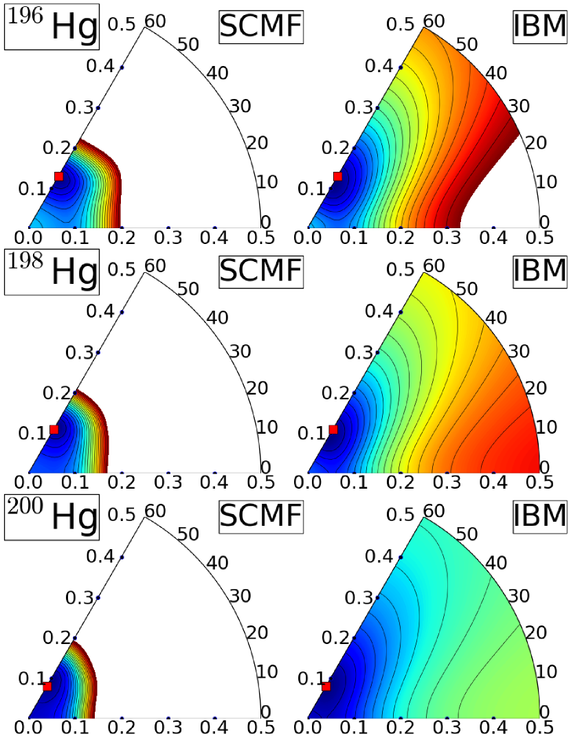
Figure 1: (Color online) The Gogny-D1M HFB and mapped IBM-2 energy surfaces in the $(\beta,\gamma)$-deformation space for the ^196-200Hg nuclei are plotted up to 5 MeV from the global minimum. The energy difference between the neighbouring contours is 250 keV. The global minimum is indicated by a filled square.

III.1 Even-even Hg isotopes

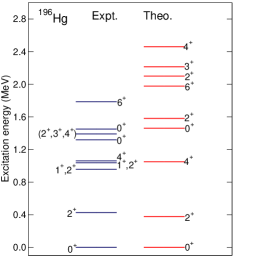
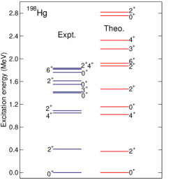
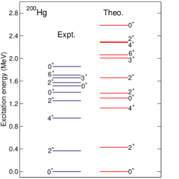
Figure 2: (Color online) Theoretical and experimental low-energy excitation spectra for the even-even nuclei ^196,198,200Hg. The experimental values are taken from NNDC compilation Brookhaven National Nuclear Data Center .

In this section, we briefly discuss relevant results for the even-even nuclei ^196,198,200Hg, which were already presented in Ref. Nomura et al. (2013). We plot in Fig. 1 the Gogny-D1M and mapped IBM-2 energy surfaces for the ^196,198,200Hg nuclei. In Fig. 1, the Gogny-D1M energy surface for the ¹⁹⁶Hg nucleus exhibits a single oblate minimum located at $\beta\approx 0.13$. The oblate minimum becomes less pronounced in ¹⁹⁸Hg and, finally, the ²⁰⁰Hg nucleus exhibits a near spherical shape with a very shallow oblate minimum at $\beta\approx 0.08$. The mapped IBM-2 energy surfaces on the right-hand side in Fig. 1 reproduce the basic features of the original Gogny-D1M ones around the global minimum, but look rather flat in the region away from the minimum. This is due to the restricted boson model space Nomura et al. (2008), which only comprises a finite number of bosons.

The calculated and experimental Brookhaven National Nuclear Data Center low-lying spectra are shown in Fig. 2. The yrast levels for all the considered even-even nuclei are described reasonably well. However, the theoretical energy levels, in particular for ^196,198Hg, look more stretched than the experimental ones. For instance, our calculation is not able to account for the excitation energy of the low-lying $0^{+}_{3}$ level of ^196,198Hg. This discrepancy could be remedied by including in the IBM-2 model space the intruder configurations that are associated with coexisting mean-field minima. These configurations are, however, not considered for the nuclei studied here Nomura et al. (2013), since their corresponding Gogny-D1M energy surfaces only exhibit a single mean-field minimum (see, Fig. 1).

III.2 Odd-mass Hg and Au isotopes

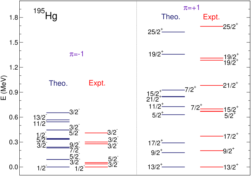
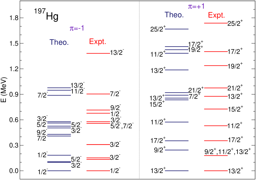
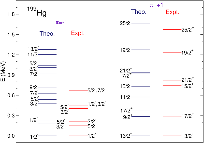
Figure 3: Same as Fig. 2, but for the odd-N nuclei ^195,197,199Hg.

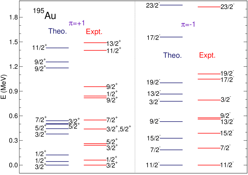
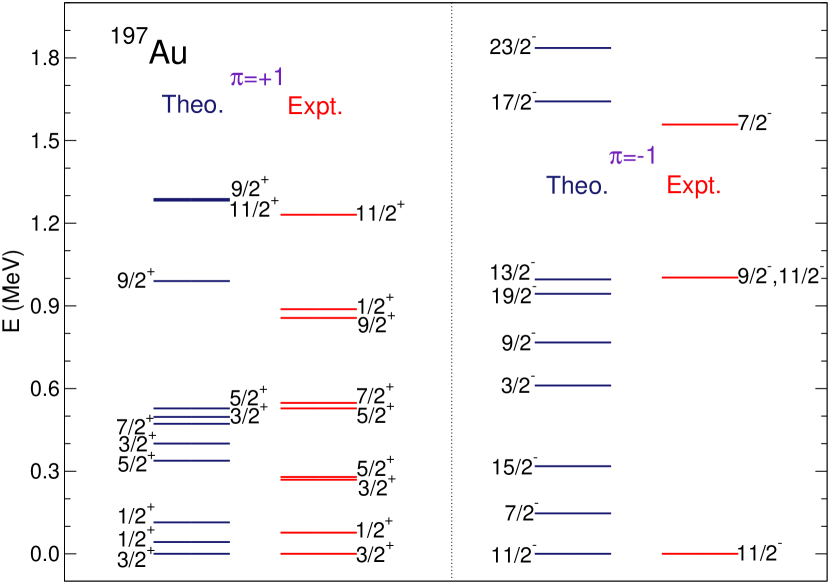
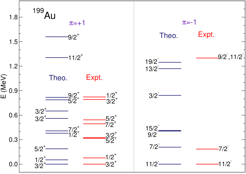
Figure 4: Same as Fig. 2, but for the odd-Z nuclei ^195,197,199Au.

Next, we discuss the spectroscopic properties of the odd-mass nuclei, obtained within the neutron-proton IBFM (IBFM-2). For the diagonalization of the IBFM-2 Hamiltonian, the computer code PBOS is used. The theoretical and experimental low-energy spectra for the odd-N nuclei ^195,197,199Hg are compared in Fig. 3. Especially for the positive-parity states, which are based on the unique-parity $\nu i_{13/2}$ configuration, the present calculation provides an excellent description of the experimental spectra for the considered odd-N nuclei, although only three parameters are involved (see, Table 3). The calculation reproduces nicely the ground-state band built on the ${13/2}^{+}_{1}$ state, which follows the $\Delta I=2$ systematic of the weak-coupling limit. For the ^195,197Hg nuclei, the calculation suggests that the negative-parity yrast states near the ground state are based mainly on the odd neutron in the $3p_{1/2}$ single-particle orbital coupled to the IBM-2 core. In the case of the nucleus ¹⁹⁹Hg, however, in most of the yrast states in the vicinity of the ground state three configurations $3p_{1/2}$, $3p_{3/2}$, and $2f_{5/2}$ are more strongly mixed than in ^195,197Hg. Such a change in the structure of the low-lying state from ^195,197Hg to ¹⁹⁹Hg, reflects the evolution of shapes in the corresponding even-even systems from ¹⁹⁸Hg (weakly oblate deformed) to ²⁰⁰Hg (nearly spherical).

In Fig. 4 we show similar plots for the odd-Z isotopes ^195,197,199Au. In general, our calculation is in a very good agreement with the experimental data. Our calculation suggests that the IBFM-2 wave functions of the lowest positive-parity states for the considered odd-Z Au nuclei are composed, with a probability of more than 80 %, of the $3s_{1/2}$ and $2d_{3/2}$ single-particle configurations, which are substantially mixed with each other. On the other hand, the $2d_{5/2}$ and $1g_{7/2}$ configurations turn out to play minor roles in describing the lowest-lying states.

We confirm that both the E2 and M1 properties of the considered odd-mass nuclei are reasonably described with the present approach.

III.3 Odd-odd Au isotopes

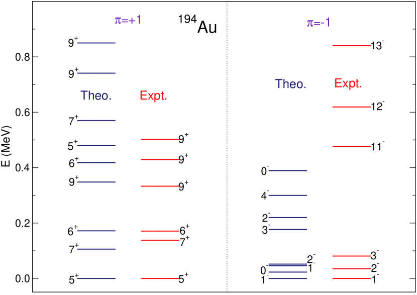
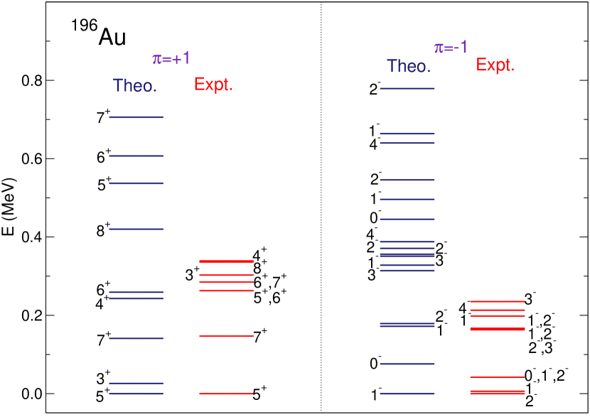
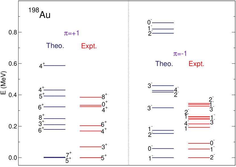
Figure 5: Same as Fig. 2, but for the odd-odd nuclei ^194,196,198Au. The experimental values are taken from Refs. Brookhaven National Nuclear Data Center ; Gao et al. (2012) (for ¹⁹⁴Au), Brookhaven National Nuclear Data Center ; Petkov et al. (2007) (for ¹⁹⁶Au), and Brookhaven National Nuclear Data Center (for ¹⁹⁸Au)

Let us now focus on the discussion of the results for the odd-odd nuclei. The low-lying spectra computed with the IBFFM-2 for the odd-odd ^194,196,198Au nuclei are depicted in Fig. 5, and compared with the experimental data Brookhaven National Nuclear Data Center .

III.3.1 ¹⁹⁴Au

Firstly, we observe that the present IBFFM-2 result for the ¹⁹⁴Au nucleus is in a very good agreement with the experimental spectra, especially for the positive-parity states. The main component ($\approx$ 72 %) in the wave functions of the lowest three positive-parity states, i.e., ${5^{+}_{1}}$, $7^{+}_{1}$, and $6^{+}_{1}$ states, is the $(\nu p_{1/2}\otimes\pi h_{11/2})$ neutron-proton pair coupled to the boson core. For the negative-parity, the energy levels near the $1^{-}$ ground state are reasonably reproduced in the present calculation. The main components of IBFFM-2 wave function of the $1^{-}$ state are the $(\nu p_{1/2}\otimes\pi s_{1/2})_{J=1^{-}}$ (17 %), and $(\nu f_{5/2}\otimes\pi s_{1/2})_{J=3^{-}}$ neutron-proton pairs (13 %). However, the calculation is not able to reproduce the experimental $11^{-}$, $12^{-}$, and $13^{-}$ levels, which are below 1 MeV excitation. The excitation energies for these states are predicted to be much larger ($>$ 3 MeV). Empirically, these higher-spin negative parity states are mainly made of the pair composed of the unique-parity orbitals, i.e., $(\nu i_{13/2}\otimes\pi h_{11/2})$ Brookhaven National Nuclear Data Center . The corresponding IBFFM-2 wave functions obtained in the present work are, however, made of the coupling between the odd neutron and proton in the normal-parity orbitals: for instance, the main components of the predicted $11^{-}_{1}$ states are the $(\nu p_{1/2}\otimes\pi s_{1/2})_{J=1^{-}}$ (35 %), $(\nu f_{5/2}\otimes\pi s_{1/2})_{J=3^{-}}$ (19 %), and $(\nu p_{1/2}\otimes\pi d_{5/2})_{J=3^{-}}$ (13 %) neutron-protons pairs.

Table 7: Calculated and experimental $B(E2)$ and $B(M1)$ transition rates (in Weisskopf units), and quadrupole $Q(I)$ (in $e$b units) and magnetic $\mu(I)$ (in $\mu_{N}$ units) moments for the odd-odd nucleus ¹⁹⁴Au. The experimental values are taken from Ref. Brookhaven National Nuclear Data Center .

	Theory	Experiment
$B(E2;6^{+}_{1}\rightarrow 5^{+}_{1})$	3.0	5(3)
$B(E2;7^{+}_{1}\rightarrow 5^{+}_{1})$	61	27(2)
$B(E2;8^{+}_{1}\rightarrow 6^{+}_{1})$	61	22(4)
$B(E2;8^{+}_{1}\rightarrow 7^{+}_{1})$	1.5	1.9(5)
$B(M1;6^{+}_{1}\rightarrow 5^{+}_{1})$	0.050	0.0010(4)
$B(M1;6^{+}_{1}\rightarrow 7^{+}_{1})$	0.020	0.0034(14)
$B(M1;8^{+}_{1}\rightarrow 7^{+}_{1})$	0.021	5$\times 10^{-5}$(2)
$Q(1^{-}_{1})$	+0.225	-0.240(9)
$\mu(1^{-}_{1})$	+1.790	+0.0763(13)

The experimental information about the electromagnetic properties is rather scarce for ¹⁹⁴Au. Nevertheless, we show in Table 7 the calculated $B(E2)$ and $B(M1)$ transition rates, and quadrupole $Q(I)$ and magnetic $\mu(I)$ moments in comparison with the available data. The predicted $B(E2)$ values seem to be qualitatively in a good agreement with the data. The calculated $B(M1)$ values are, however, too large as compared to the experimental values. The sign of the predicted $Q(1^{-})$ moment is opposite to that given by the experiment.

III.3.2 ¹⁹⁶Au

From the comparison of energy levels of the odd-odd nucleus ¹⁹⁶Au, shown in Fig. 5, one concludes that the calculation is able to reproduce both the experimental positive- and negative-parity levels reasonably well. The calculated low-lying positive-parity states for ¹⁹⁶Au are similar in structure to those for ¹⁹⁴Au: 67 % and 66 % of the predicted $5^{+}_{1}$ and $7^{+}_{1}$ states are dominated by the $(\nu p_{1/2}\otimes h_{11/2})_{J=5^{+}}$ pair component, respectively. The spin of the calculated lowest negative parity state is $I=1^{-}$. This is at variance with the experiment, although the experimental $1^{-}_{1}$ level is only 6 keV above the $2^{-}_{1}$ ground state. Furthermore, the present calculation considerably overestimates the $2^{-}_{1}$ energy level. The non-negligible components ($>$ 10 %) of the corresponding IBFFM-2 wave functions for the $2^{-}_{1}$ and $1^{-}_{1}$ states are the following: $(\nu p_{1/2}\otimes\pi d_{3/2})_{J=2^{-}}$ (24 %), $(\nu p_{1/2}\otimes\pi s_{1/2})_{J=1^{-}}$ (11 %), and $(\nu f_{5/2}\otimes\pi s_{1/2})_{J=2^{-}}$ (11 %) for the $2^{-}_{1}$ state, and $(\nu p_{1/2}\otimes\pi s_{1/2})_{J=1^{-}}$ (38 %) and $(\nu p_{1/2}\otimes\pi d_{3/2})_{J=1^{-}}$ (10 %) for the $1^{-}_{1}$ state.

Table 8: Same as Table 7, but for the nucleus ¹⁹⁶Au. The experimental values are taken from Refs. Brookhaven National Nuclear Data Center ; Petkov et al. (2007)

	Theory	Experiment
$B(E2;6^{+}_{1}\rightarrow 5^{+}_{1})$	2.1	$>$0.064
$B(E2;6^{+}_{2}\rightarrow 5^{+}_{1})$	7.7	$>$0.0068
$B(E2;7^{+}_{1}\rightarrow 5^{+}_{1})$	50	51(6)
$B(E2;7^{+}_{2}\rightarrow 5^{+}_{1})$	0.24	$>$0.064
$B(E2;8^{+}_{1}\rightarrow 6^{+}_{1})$	51	0.77(39)
$B(E2;8^{+}_{1}\rightarrow 6^{+}_{2})$	0.28	20(7)
$B(E2;8^{+}_{1}\rightarrow 7^{+}_{1})$	1.0	0.76$\times 10^{-1}$(26)
$B(E2;8^{+}_{1}\rightarrow 7^{+}_{2})$	0.018	0.77(39)
$B(E2;3^{-}_{2}\rightarrow 1^{-}_{1})$	11	$>$6.5
$B(E2;4^{-}_{1}\rightarrow 2^{-}_{1})$	21	9.7(2.4)
$B(E2;4^{-}_{1}\rightarrow 2^{-}_{2})$	1.8	13.2(13.2)
$B(E2;4^{-}_{1}\rightarrow 3^{-}_{1})$	0.34	13.2(13.2)
$B(M1;6^{+}_{1}\rightarrow 7^{+}_{1})$	0.029	3.5$\times 10^{-5}$
$B(M1;6^{+}_{2}\rightarrow 6^{+}_{1})$	0.077	$>$0.00016
$B(M1;6^{+}_{2}\rightarrow 7^{+}_{1})$	0.14	3.5$\times 10^{-5}$
$B(M1;6^{+}_{2}\rightarrow 7^{+}_{2})$	0.050	$>$0.00016
$B(M1;7^{+}_{2}\rightarrow 7^{+}_{1})$	0.0053	3.5$\times 10^{-5}$
$B(M1;8^{+}_{1}\rightarrow 7^{+}_{1})$	0.022	0.49$\times 10^{-3}$(5)
$B(M1;3^{-}_{2}\rightarrow 2^{-}_{1})$	0.17	$>$0.0045
$Q(2^{-}_{1})$	+0.495	0.81(7)
$\mu(2^{-}_{1})$	+0.197	+0.580(15)

Table 8 exhibits the calculated and experimental electromagnetic properties. Regarding the $B(E2)$ rates, our results are in a reasonable agreement with the experiment. However, similarly to ¹⁹⁶Au the calculated $B(M1)$ values are generally much larger than the experimental values. A number of experimental $B(E2)$ and $B(M1)$ transition rates from the $1^{-}$ state at the excitation energy of $E_{\text{x}}=298.5$ keV are available Petkov et al. (2007). However, there are also too many experimental $1^{-}$ states below 298.5 keV, and it is not clear which theoretical $1^{-}$ state corresponds to the experimental one observed at $E_{\text{x}}=298.5$ keV. For this reason, we do not compare our results with the experimental $B(E2)$ and $B(M1)$ transitions rates from the $1^{-}(298.5\,\text{keV})$ state.

III.3.3 ¹⁹⁸Au

As one sees from the comparison between the theoretical and experimental low-energy spectra for the odd-odd nucleus ¹⁹⁸Au in Fig. 5, the description of the positive-parity states is generally good. As in the case of ¹⁹⁶Au, however, our calculation fails to reproduce the spin of the lowest negative-parity state. The structure of the $2^{-}_{1}$ and $1^{-}_{1}$ wave functions for ¹⁹⁸Au turn out to be rather similar to those of ¹⁹⁶Au, that is, $(\nu p_{1/2}\otimes\pi d_{3/2})_{J=2^{-}}$ (26 %), $(\nu p_{1/2}\otimes\pi s_{1/2})_{J=1^{-}}$ (19 %), and $(\nu p_{1/2}\otimes\pi s_{1/2})_{J=0^{-}}$ (12 %) for the $2^{-}_{1}$ state, and $(\nu p_{1/2}\otimes\pi s_{1/2})_{J=1^{-}}$ (41 %) and $(\nu p_{1/2}\otimes\pi d_{3/2})_{J=1^{-}}$ (13 %) for the $1^{-}_{1}$ state. The previous IBFFM calculation of Lopac et al. (1986) obtains an excellent description of both the positive- and negative-parity levels. The IBFFM wave functions they obtained are predominantly described by the $(\nu p_{1/2}\otimes\pi d_{3/2})_{J=2^{-}}$ component ($>$ 70 %) for the $2^{-}_{1}$ state, and $(\nu p_{1/2}\otimes\pi d_{3/2})_{J=1^{-}}$ (50 %) for the $1^{-}_{1}$ state. The difference between our result and that of Lopac et al. (1986) could be accounted for by the different single-particle energies used in each study. In the present calculation, the $2d_{3/2}$ single-particle orbital is about 0.9 MeV above the $3s_{1/2}$ (see, Table 6). On the other hand, in Lopac et al. (1986) the $2d_{3/2}$ orbital is below the $3s_{1/2}$ one and, consequently, the $\pi d_{3/2}$ single-particle configuration plays a more dominant role in low-energy region than in our calculation.

Table 9: Same as Table 7, but for the nucleus ¹⁹⁸Au.

	Theory	Experiment
$B(E2;1^{-}_{2}\rightarrow 2^{-}_{1})$	6.7	2.2(7)
$B(E2;2^{-}_{3}\rightarrow 4^{-}_{1})$	0.049	$>$64
$B(E2;3^{-}_{1}\rightarrow 1^{-}_{1})$	8.3	$>$26
$B(E2;3^{-}_{1}\rightarrow 2^{-}_{1})$	2.1	$>$13
$B(E2;4^{-}_{1}\rightarrow 2^{-}_{1})$	13	35(18)
$B(M1;1^{-}_{2}\rightarrow 0^{-}_{1})$	0.015	0.0032(10)
$B(M1;1^{-}_{2}\rightarrow 1^{-}_{1})$	0.0049	0.00024(8)
$B(M1;1^{-}_{3}\rightarrow 0^{-}_{1})$	0.00067	7.4$\times 10^{-5}$(24)
$B(M1;1^{-}_{3}\rightarrow 1^{-}_{1})$	0.00051	0.0017(5)
$B(M1;1^{-}_{4}\rightarrow 0^{-}_{1})$	8.2$\times 10^{-5}$	$>$0.0084
$B(M1;1^{-}_{4}\rightarrow 2^{-}_{1})$	0.0021	$>$9.9$\times 10^{-6}$
$B(M1;1^{-}_{5}\rightarrow 1^{-}_{1})$	0.022	$>$0.00029
$B(M1;1^{-}_{5}\rightarrow 1^{-}_{2})$	0.042	$>$0.0042
$B(M1;1^{-}_{6}\rightarrow 0^{-}_{1})$	0.0013	$>$0.00025
$B(M1;1^{-}_{6}\rightarrow 1^{-}_{4})$	0.10	$>$0.015
$B(M1;1^{-}_{6}\rightarrow 2^{-}_{1})$	0.0010	$>$5.6$\times 10^{-5}$
$B(M1;2^{-}_{2}\rightarrow 1^{-}_{1})$	0.064	$>$0.00033
$B(M1;2^{-}_{2}\rightarrow 2^{-}_{1})$	0.024	$>$0.0037
$B(M1;2^{-}_{3}\rightarrow 1^{-}_{2})$	4.5$\times 10^{-6}$	$>$0.00065
$B(M1;2^{-}_{3}\rightarrow 1^{-}_{3})$	0.024	$>$0.0048
$B(M1;2^{-}_{3}\rightarrow 2^{-}_{1})$	8.5$\times 10^{-5}$	$>$0.00042
$B(M1;2^{-}_{4}\rightarrow 1^{-}_{4})$	0.0015	$>$0.015
$B(M1;3^{-}_{1}\rightarrow 2^{-}_{1})$	0.42	$>$0.0019
$B(M1;3^{-}_{2}\rightarrow 2^{-}_{1})$	0.0042	$>$0.0026
$Q(2^{-}_{1})$	+0.373	+0.64(2)
$\mu(5^{+}_{1})$	+4.398	-1.11(2)
$\mu(2^{-}_{1})$	+0.334	+0.5934(4)

In Table 9 the calculated $B(E2)$ values for ¹⁹⁸Au are, in general, in good agreement with the experiment. We also present the calculated $B(M1)$, but for most of the available data only a lower limit for this quantity is known. The calculated magnetic moment of the $5^{+}_{1}$ state, $\mu(5^{+}_{1})$, has the opposite sign and is a factor of 4 larger in magnitude than the experimental one. Similar results have been obtained for the ^194,196Au nuclei as we obtain $\mu(5^{+}_{1})\approx 5$ $\mu_{N}$. As already mentioned, the $5^{+}_{1}$ states obtained in the present calculation for the considered odd-odd Au nuclei are dominated by the $(\nu p_{1/2}\otimes\pi h_{11/2})_{J=5^{+}}$ neutron-proton pair configuration, and the predicted $\mu(5^{+}_{1})$ moments are mostly accounted for by this configuration, in particular, by the odd-proton part of the M1 matrix element, which takes large positive value. On the other hand, empirical studies for the low-lying level structure of ¹⁹⁴Au Pakkanen et al. (1977); Gao et al. (2012) assume the $5^{+}_{1}$ state and the band built on it to be based mainly on the $(\nu i_{13/2}^{-1}\otimes\pi d_{3/2}^{-1})_{J=5^{+}}$ configuration, leading to the correct sign of the $\mu(5^{+}_{1})$ moment.

IV Summary and concluding remarks

In this work, we extend the recently developed method of Ref. Nomura et al. (2016a) for calculating the spectroscopy of odd-mass nuclei to odd-odd systems. The $(\beta,\gamma)$-deformation energy surfaces of the even-even core nuclei, and spherical single-particle energies and occupation probabilities of the odd neutron and the odd proton are calculated by the constrained HFB method based on the Gogny D1M EDF. These quantities are then used as microscopic input to build most of the different terms of the IBFFM-2 Hamiltonian. The strength parameters for the boson-fermion interaction terms in the IBFFM-2 Hamiltonian are taken from those of the neighbouring odd-mass nuclei. Two coefficients in the residual interaction between odd neutron and proton are the only new parameters, and are determined as to reproduce the low-energy levels of each odd-odd nucleus. In this way, we are able to reduce significantly the number of free parameters in the IBFFM-2 framework. It is shown that the method provides a reasonable description of low-energy spectra and electromagnetic properties of the odd-odd nuclei ^194,196,198Au. Even though a few strength parameters in the boson-fermion and fermion-fermion interactions are treated as free parameters, the method developed in this paper, as well as in Ref. Nomura et al. (2016a), in which the even-even IBM-core Hamiltonian is determined fully microscopically and only one or two unpaired nucleon degrees of freedom are added via the particle-boson coupling, allows for a simultaneous description of a large number of even-even, odd-mass, and odd-odd medium-mass and heavy nuclei.