Multiplicity spectra in $e^{+}e^{-}$ and $\overline{p}p$ collisions in terms of Tsallis and Weibull distributions.

Abstract

Charged hadron production in the $e^{+}e^{-}$ annihilations at 91 to 206 GeV in full phase space and in $\overline{p}p$ collisions at 200 to 900 GeV collision energies are studied using non-extensive Tsallis and stochastic Weibull probability distributions. The Tsallis distribution shows better description of the data than the Weibull distribution. The 2-jet modification of the statistical distribution is applied to describe $e^{+}e^{-}$ data. The main features of these distributions can be described by a two-component model with soft, collective interactions at low transverse energy and hard, constituent interactions dominating at high transverse energy. This modification is found to give much better description than a full-sample fit, and again Tsallis function is found to better describe the data than the Weibull one pointing at the non-extensive character of the multiparticle production process.

PACS numbers: 5.90.+m, 12.40.Fe, 13.66.Bc

1 Introduction

Charged hadron production in high energy particle interactions can be understood in terms of several theoretical and phenomenological models derived from statistics, empirical relationships, phenomenological concepts or pure theoretical cosiderations [Kanki-Gros]. To understand the particle production mechanism, some models have used ensemble theory from statistical mechanics to extract information from dynamical fluctuations as a key source of inputs to study the multiplicity patterns. Several distributions based on the statistical analyses have been derived for the understanding of particle production and the multiplicity distributions. However, it was realized that data on many single particle distributions deviate from the distributions expected from the statistical models, based on standard statistical mechanics of Boltzman-Gibbs which treats the entropy as an extensive property. This initiated the idea of including modifications to include possible intrinsic, non-statistical fluctuations. These were identified as the source of the deviations. Such fluctuations are important as possible signals of phase transition(s) taking place in an hadronizing system.

The Tsallis formalism was introduced three decades ago [TS1]. It is a non-extensive generalization of the statistical mechanics and has been very successful in describing very different physical systems in terms of statistical approach, including multiparticle production processes at lower energies. Specially designed to include self-similar systems and systems with long range interactions, it is a reasonable choice to study hadronisation process. The collisions at collider experiments are expected to fall in this category. Thus the Tsallis statistical approach [TS2-JC], was successfully used for multiparticle production processes. The new approach in the Tsallis $q$-statistics which includes entropy as a non-extensive property to describe the particle production has not been tested with the highest energy data from $e^{+}e^{-}$ collisions and $\overline{p}p$ collisions, though this has been used to explain heavy-ion and some $pp$ collision data, see references [Zhang-Mar]. Most of these studies have focussed on the $p_{T}$ spectra of the hadrons.

The non-extensive part of entropy is quantified in terms of a parameter $q$, the entropic index in the Tsallis function and envisaged that it should have a value greater than unity. The total Tsallis entropy of two sub-systems $a$ and $b$ is not equal to the sum of the entropies of the subsystems, but is given by;

$$S_{q}(a,b)=S_{a}+S_{b}+(1-q)S_{a}S_{b}\,$$ (1)

In Tsallis $q$-statistics probability is calculated by using the partition function Z, as

$$P_{N}=\frac{Z^{N}_{q}}{Z}$$ (2)

where Z represents the total partition function and $Z^{N}_{q}$ represents partition function at a particular multiplicity, of the grand canonical ensemble of gas consisting of $N$ particles. $\bar{N}$, the average number of particles, is given by

$$\bar{N}=Vn[1+(q-1)\lambda(Vn\lambda-1)-2v_{0}n]$$ (3)

$K$-parameter is related to $q$ and excluded volume $v_{0}$, by

$$\frac{1}{K}=(q-1)\lambda^{2}-2\frac{v_{0}}{V}$$ (4)

where $V$ is the volume containing $N$ particles, $\lambda$ is related to the temperature through the parameter $\beta$ as;

$$\lambda(\beta,\mu)=-\frac{\beta}{n}\frac{\partial n}{\partial\beta}$$ (5)

Details of the Tsallis distribution and how to find the probability distribution can be obtained from [TS2]. In the hadron-hadron interactions, the dynamics of particle production is centered around the fragmentation process, partons are produced at the intermediate stage which quickly undergo fragmentation into hadrons.

A description of the fragmentation process can also be given in terms of Weibull distribution [Wei] in which it has been shown that result of a single event fragmentation leading to a branching tree of cracks in the materials that show fractal behaviour [Brown] and can be described by a Weibull-like distribution. This is related to the particle number distribution developed during the fragmentation, the so called multiplicity distribution in case of particle collisions.

Weibull distribution has been studied to describe multiplicity distributions in $e^{+}e^{-}$ collisions up to 91 GeV [Wei] and also for $ep$ collisions. Weibull parametrization of the multiplicity distribution has also been used to describe the multi-dimensional fluctuations and genuine multi-particle correlations in $e^{+}e^{-}\rightarrow Z^{0}\rightarrow hadrons$ [Edward,Nayak].

The Tsallis distribution [TS1,TS2] and the Weibull distribution [Wei] are based on the concepts of statistical mechanics and stochasticity. The simplicity of these statistically inspired models and the ease of application to data, is the beauty of the analyses. Nowadays the statistical approach is a standard procedure used to model high energy multiparticle production processes [Ga].

In the present work, we focus on the multiplicity distributions, in full phase space in $e^{+}e^{-}$ annihilations up to the highest available center-of-mass energies and in $\overline{p}p$ collisions at energies ranging from 200 to 900 GeV in restricted rapidity windows. The presence of a shoulder structure in the multiplicity distribution was observed in $e^{+}e^{-}$ at collision energy of $\sqrt{s}$=91 GeV [KT2,OPAL91] and in $\overline{p}p$ data at 900 GeV [UA51] and at $\sqrt{s}$=1800 GeV [Rimo]. The data from LEP2 also confirmed the presence of the shoulder structure at higher then $Z^{0}$ energies [OPAL161,OPAL172]. It is the higher energy data where the shoulder structure becomes more pronounced.

Recently, we have studied [MK] the data in terms of the Tsallis distribution and the Weibull distribution at lower energies in full phase space and in different rapidity windows. To study the high energy data and to take into account the shoulder structure, we implement a 2-jet modification to improve the comparison between the predicted and the experimental values. The two-component approach has been suggested earlier in reference [Gov]. The study indicates that the Tsallis function is able to reproduce the experimental results far better than the Weibull one. Further analysis is performed here to assert our conclusions.

In Section 2, an outline of probability distribution functions of Tsallis and Weibull distrbutions and their modified forms are given. Details along with the references can be found in [TS2]. 2-jet fractions denoted by $\alpha$ at various energies have been taken from the references [OPAL161,OPAL172,Alex-L3] obtained by OPAL and L3/ALEPH experiments. The 2-jet data samples considered are only those for $e^{+}e^{-}$ collisions, and no 2-jet modification is made to study $\overline{p}p$ data as no 2-jet data-samples being available for these collisions. Section 3 presents the analyses of experimental data and the results obtained by the two approaches. Discussion and conclusion are given in Section 4.

2 Tsallis and Weibull distributions and their 2-jet modification

2.1 Tsallis and its 2-jet modification

Details and the method of calculating the partition function for $N$ particles, in the Grand Canonical Ensemble, Tsallis $q$-index and Tsallis $N$-particle probability distribution can be obtained from [TS2]. The probability is calculated by using the partition function $Z$ , as

$$P_{N}=\frac{Z^{N}_{q}}{Z}$$ (6)

where $Z$ represents the total partition function and $Z^{N}_{q}$ represents partition function at a particular multiplicity $N$.

The probability distribution for the 2-jet modified distribution is calculated by adding a weighted superposition of multiplicity in 2-jet and in multi-jet events as follows;

$$P_{N}(\alpha:\bar{n_{1}},V_{1},v_{01},q_{1}:\bar{n_{2}},V_{2},v_{02},q_{2})=\\ \alpha P_{N}^{\rm 2-jet}+\\ (1-\alpha)P_{N}^{\rm multi-jet}.$$ (7)

where $\alpha$ is a weight factor which gives 2-jet fraction and is determined from a jet finding algorithm.

2.2 Weibull and its 2-jet modification

The probability density function of a Weibull random variable is;

$$P_{N}(N,\lambda,k)=\frac{k}{\lambda}(\frac{N}{\lambda})^{(k-1)}exp^{-(\frac{N}{\lambda})^{k}},\hskip 11.38092ptwhereN\geq 0.$$ (8)

Where $\lambda>0$ is the scale parameter and $k>0$ is the shape parameter. These two parameters for the distribution are related to the mean of the function, as

$$\bar{N}=\lambda\Gamma(1+1/k)$$ (9)

The modified Weibull function can be obtained by the weighted superposition of the two Weibull distributions, as above, namely;

$$P_{N}(\alpha:N_{1},\lambda_{1},k_{1};N_{2},\lambda_{2},k_{2})=\\ \alpha P_{N}^{\rm 2-jet}+\\ (1-\alpha)P_{N}^{\rm multi-jet}.$$ (10)

3 Results

The experimental data on $e^{+}e^{-}$ annihilation at different collision energies by two experiments are analysed here. The details of the data from the L3 [L3] and OPAL [OPAL91,OPAL161,OPAL172,Alex,Acc] experiments at different energies between $\sqrt{s}$ = 91 to 206 GeV in the full phase space are given in Table 1. For comparison, we also analyse data from $\overline{p}p$ collisions at energies ranging from 200 to 900 GeV in restricted rapidity windows from the UA5 collaboration [UA51,UA52] as given in Table 2. The experimental distributions are fitted with the predictions from two probability functions, as described above.

3.1 one-component Tsallis versus Weibull functions

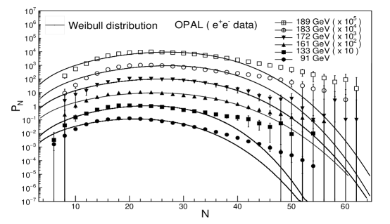
Figure 2: The charged multiplicity distributions measured in $e^{+}e^{-}$ annihilation by the OPAL experiment and the fits by the Tsallis distribution and Weibull distribution.

The probability distribution for Tsallis function is calculated from equation (2) and Weibull function from eqns. (8) and (9) and applied to fit the $e^{+}e^{-}$ data in full phase space, as shown in Figures 1 and 2. Parameters of the fits and $\chi^{2}/ndf$ values are given in Table 2 and the corresponding p values are given Table 3.  We find that overall, Weibull distribution fails to reproduce the data, particularly in the high multiplicity regions, while Tsallis distribution shows good fit in full phase space.

One observes that the $\chi^{2}/ndf$ values are significantly lower for the Tsallis fits in comparison to the Weibull fits. This is true for all energies. A careful examination of the $p$ values from Table 3 shows that for the data from L3 experiment at all energies from 130 to 206 GeV, the Weibull fits are statistically excluded with $CL<0.1\%$. While for the Tsallis fits for the data only at 200.2 and 206.2 are statistically excluded with $CL<0.1\%$ and is good for all other energies with $CL>0.1\%$.  For the data from OPAL experiment, the Weibull fit is statistically excluded systematically for all energies between 91 to 189 GeV with $CL<0.1\%$ except being good for energy 172 GeV. Again Tsallis fit is excluded only for 91 GeV data and remains a good fit for all energies from 133 to 189 GeV with $CL>0.1\%$. A comparison of the $\chi^{2}/ndf$ and $p$ values in Table 3 shows that $\chi^{2}/ndf$ values for the Tsallis distributions are lower by several orders, confirming that Tsallis distribution fits the data far better than Weibull distribution.

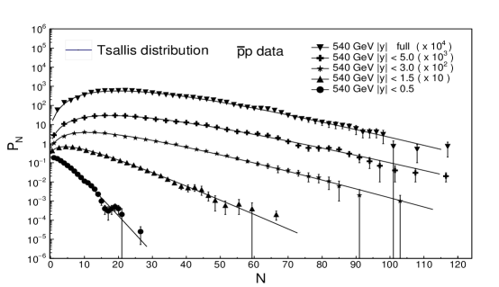
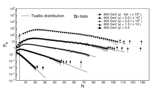
Figure 3: The charged multiplicity distribution measured in $\overline{p}p$ interactions by the UA5 experiment and the fits by the Tsallis distributions.

Figures 3 and 4 show the Tsallis and Weibull fits to the data on $\overline{p}p$ collisions from UA5 collaboration at energies ranging from 200 to 900 GeV in restricted rapidity windows as well as in full phase space. The parameters of the fits are listed in Table 4. Again the Tsallis distribution shows very good fits at all energies and all rapidities with statistically significant $p$ values $\chi^{2}/ndf$ values in comparison to the Weibull distribution, as shown in Table 5. In each of the data samples of $e^{+}e^{-}$, for the Weibull distribution, $\lambda$ values increase with energy and in case of $\overline{p}p$ collisions these increase with energy as well as with the size of the central rapidity interval. Similarly for Tsallis distribution, the $q$ value which measures the entropic index, of the Tsallis statistics is consistently higher than 1 in each of the above mentioned cases. This confirms the property of the non-extensivity in the data as proposed by the Tsallis q-statistics.

3.2 Modified Tsallis versus modified Weibull distributions

As it is observed above, in the case of the Weibull fits, the description is good enough only for the data at some energies, while it gets quite high $\chi^{2}/ndf$ values for the rest. Also, though the Tsallis fits are better than the Weibull ones, there is still a room for improvements. Following the two-component approach suggested by Giovannini [Gov] we consider the two-components of the modified Tsallis distribution and modified Weibull distribution for $e^{+}e^{-}$ data. The probability functions for the two cases can be derived from the equations (7) and (10). The fit parameters, $\chi^{2}/ndf$ and $p$ values for both modified Weibull and modified Tsallis distributions are given in Tables 3, 6 and 7. Figure 5 and 6 show the modified distributions for the L3 and OPAL data.

One can see that values given in Table 3 show that following the two-component fits improve substantially the description. The modified Tsallis distributions describe the data extremely well at all energies. For the modified Weibull distribution, though the $\chi^{2}/ndf$ values improve substantially, it still fails for energies above the $Z^{0}$ peak, namely 161, 188.6, 189 and 206.2 GeV data samples for which $CL<0.1\%$.

Figure 7 shows plots of the $q$, $q_{1}$ and $q_{2}$ values estimated from the Tsallis fits and modified Tsallis fits. The bands shown are the confidence bands. The mean values are $q=1.388\pm 0.095$, $q_{1}=1.077\pm 0.017$ and $q_{2}=1.489\pm 0.100$. The figure shows that the $q$ values in both the cases of the Tsallis and modified Tsallis fits, exceed unity, emphasising the non-extensive nature of the Tsallis entropy.

Figure 8 shows the dependence of $\lambda$, $\lambda_{1}$, $\lambda_{2}$, on c.m.s energy of $e^{+}e^{-}$ collisions. As the parameter $\lambda$ is connected with the average multiplicity, it is expected to increase with the energy of collision and hence charged multiplicity. The dependence of $\lambda$ on c.m. energy $\sqrt{s}$ is studied as a power law $\lambda=A\sqrt{s}^{B}$, $A$ and $B$ are the fit parameters. One finds the following values of the parameters $A$ and $B$:

for $\lambda$ : $A=10.05\pm 0.99\hskip 14.22636pt{\rm and}\hskip 14.22636ptB=0.20\pm 0.019$,

for $\lambda_{1}$ : $A=5.50\pm 1.26\hskip 14.22636pt{\rm and}\hskip 14.22636ptB=0.29\pm 0.04$,

and for $\lambda_{2}$ : $A=3.58\pm 0.62\hskip 14.22636pt{\rm and}\hskip 14.22636ptB=0.45\pm 0.03$.

The modified analyses for $\overline{p}p$ could not be carried out as the 2-jet fractions for these data in different rapidity intervals as well as in the full phase space are not available.

3.3 Discussion

The standard Boltzmann-Gibbs statistics, with $q$=1 produces a distribution which is not consistent with the experimental data at high energy and at high multiplicity tail. It is known that it could lead to unphysical results for systems having long-range interactions. This is the non perturbative regime of QCD which plays an important role in hadronization. The large particle density fluctuations [Ada,Bur] present in hadron production, which could not be explained, mandated an alternative formalism to be developed. One such case is the Tsallis formalism.

In the Tsallis distribution, $K$-parameter in eq.(4) is related to $q$, the entropic index, $v_{0}$, the excluded volume associated to a particle and the volume of the system. The detailed relationship can be found in [TS2]. The $K$-parameter measures the deviation from Poisson distribution caused by resonance decay and charge conservation and is related to the variance. The definition of $K$ is motivated by the $k$ parameter of a negative binomial distribution. The Tsallis statistics for $q>1$ with excluded volume $v_{0}$ causes a substantial broadening of the distribution, taking it much closer to the data. Thus the role of $K$-parameter is crucial to the value of entropic index, $q$. In some analyses the excluded volume is fixed between 0.3-0.4 $fm^{3}$. The corresponding value of volume $V$ then varies from few $fm^{3}$ to few tens of $fm^{3}$ [TS2].

The smooth increase of $q$ with the center of mass energy can be understood as the expected increase of the influence of the partonic interactions among the hadronic particles produced in the event.

Table 2 shows that the shape parameter $k$ for the Weibull function determines the shape of the distribution. For the highest LEP energy range, the value of $k$ does not change much within limits of errors, as can be seen in Tables 2 and  6. This behaviour is related to the soft gluon emission and subsequent hadronisation. Within a given rapidity interval, the value of $k$ decreases slightly with increasing energy. However, it increases considerably from smaller to larger rapidity intervals, as can be seen in Table 4. The scale parameter $\lambda$ of the Weibull distribution determines the width of the distribution. Larger value of scale parameter produces a broader distribution. This again is observed in Tables 2 and 4. The width of the probability distribution depends upon c.m. energy. At higher collision energies, more number of high multiplicity events are produced and the multiplicity distribution becomes broader. As a result, $\lambda$ increases to compensate for the width. This trend is endorsed by $\lambda$ values in the two Tables. Similar results are observed from the modified Weibull fit distribution parameters in Table 6 where $\lambda$ values increase systematically from lower to higher rapidity windows.

For various energies, it is shown that by appropriately weighting the multiplicity distribution with the 2-jet fraction in $e^{+}e^{-}$ collisions at $\sqrt{s}$ = 91 to 206 GeV, both the Tsallis distributions and the Weibull distributions substantially improve the agreement with the data giving the statistically significant results. These modified Tsallis distributions reproduce the data well with $CL>0.1\%$ for all energies, from both the L3 and OPAL experiments. The modified Weibull distributions, also improve the fits by several orders, but fail to describe the data at most of the energy points, as can be observed from $p$ values in Table 3

The highest energy data sets have typically low statistics, due to which fit parameters suffer from large errors, especially for modified Tsallis distribution. Nevertheless the present detailed analysis establishes that the performance of the Tsallis function is better than Weibull function. The $q$ value known as entropic index for the Tsallis distribution, accounts for the non-extensive thermo-statistical effects in hadron production and is expected to exceed unity in the Tsallis statistics. This is confirmed from the mean values of $q$, as measured for the total sample of events, events with two-jets and events with multijets. The behaviour is found to be more pronounced in the events with higher multiplicity, as evident from the difference in q-values for 2-jet and multi-jet components. The analyses for the Tsallis distribution and the Weibull distribution for $\overline{p}p$ collisions from 200 to 900 in full phase space as well as in restricted rapidity windows have also been done. It is found that the Weibull distribution is excluded in full phase space at all energies and in several rapidity windows. Whereas for the Tsallis, it is acceptable at most of the energy and rapidity values with the exception of 900 GeV in full phase space and at 540 GeV for $|y|<0.5$ GeV where the fits have $CL<0.1\%$. For Tsallis distribution, in each case $q$ value exceeds unity, emphasising the non-extensive nature of the Tsallis entropy.

4 Conclusions

Analyses of the multiplicity distributions measured in $e^{+}e^{-}$ collisions at LEP at energies, $\sqrt{s}$=91 to 206 GeV and in $\overline{p}p$ collisions at 200 to 900 GeV have been done in the context of Weibull and Tsallis distributions. It is observed that the the Weibull fits for the data from L3 experiment at all energies from 130.1 GeV to 206.2 GeV for the $e^{+}e^{-}$ collisions are statistically excluded with $CL<0.1\%$, and for the Tsallis fits the data only at 200.2 GeV and 206.2 GeV are statistically excluded and are good for all other energies. For the data from OPAL experiment, Weibull fits are statistically excluded for all energies between 91 GeV to 189 GeV with $CL<0.1\%$ in $e^{+}e^{-}$ annihilation, except the 172 GeV data. In contrast, the Tsallis fits are excluded only for energy at 91 GeV and remain good for all other energies of 133 GeV to 189 GeV. Tsallis non-extensive statistics gives a good description of the particle production in high energy collisions.

Acknowledgement: We thank Professor Edward K.G. Sarkisyan for important suggestions and comments. One of the authors, S. Sharma is grateful to the Department of Science and Technology, Government of India for the fellowship grant.

Figure 1: The charged multiplicity distributions measured in $e^{+}e^{-}$ annihilation by the L3 experiment and the fits by the Tsallis distribution and Weibull distribution.

Figure 4: The charged multiplicity distribution measured in $\overline{p}p$ interactions by the UA5 experiment and the fits by the Weibull distributions.

Figure 5: The charged particle multiplicity distributions measured in $e^{+}e^{-}$ collisions by the L3 experiment with the fits by the modified Tsallis and Weibull distributions.

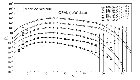
Figure 6: The charged particle multiplicity distributions measured in $e^{+}e^{-}$ collisions by the OPAL experiment with the fits by the modified Tsallis and Weibull distributions.

Figure 7: The Tsallis $q$, $q_{1}$ and $q_{2}$ fit parameters obtained for $e^{+}e^{-}$ data.

Figure 8: The Weibull distribution $\lambda$, $\lambda_{1}$ and $\lambda_{2}$ fit parameters obtained for $e^{+}e^{-}$ annihilation as a function of collision energy. The lines represent the power law fits.

Description of the data samples used in the analysis.$\alpha$-values represent the fraction of the 2-jet events in the samples as obtained by the measurements. Energy Experiment [Reference] No. of events $\alpha$(2-jet fraction) Reference (GeV) for $\alpha$ $e^{+}e^{-}$ 91 OPAL [OPAL91] 82941 0.657 [OPAL172] 133 ” [Alex] 13665 0.662 [Alex] 161 ” [OPAL161] 1336 0.635 [OPAL161] 172 ” [OPAL172] 228 0.666 [Acc] 183 ” ” 1098 0.675 [Jon] 189 ” ” 3277 0.662 [OPAL172] 130.1 L3 [L3] 556 0.654 [L3] 136.1 ” ” 414 0.649 ” 172.3 ” ” 325 0.657 ” 182.8 ” ” 1500 0.668 ” 188.6 ” ” 4479 0.670 ” 194.4 ” ” 2403 0.679 ” 200.2 ” ” 2456 0.661 ” 206.2 ” ” 4146 0.666 ” $\overline{p}p$ 200 UA5 [UA51] 4156 – – 540 UA5 [UA52] 6839 – – 900 UA5 [UA51] 7344 – –

The parameters of the Weibull and the Tsallis functions for $e^{+}e^{-}$ collisions. Energy Weibull distribution Tsallis distribution (GeV) $k$ $\lambda$ $\chi^{2}/ndf$ $K$ $q$ $\chi^{2}/ndf$ 91 3.548 $\pm$ 0.033 23.197 $\pm$ 0.073 434.91/22 21.397 $\pm$ 0.670 1.751 $\pm$ 0.325 33.13/20 133 4.029 $\pm$ 0.122 25.239 $\pm$ 0.374 66.88/22 19.891 $\pm$ 2.251 1.405 $\pm$ 0.562 12.67/20 161 3.542 $\pm$ 0.098 27.174 $\pm$ 0.300 48.11/22 17.983 $\pm$ 1.587 1.340 $\pm$ 0.093 5.81/20 172 3.813 $\pm$ 0.162 27.942 $\pm$ 0.479 17.87/22 21.274 $\pm$ 3.003 1.097 $\pm$ 0.075 3.94/20 183 4.069 $\pm$ 0.088 29.117 $\pm$ 0.277 159.61/25 19.749 $\pm$ 1.339 1.056 $\pm$ 0.023 35.13/23 189 3.994 $\pm$ 0.058 29.018 $\pm$ 0.197 183.63/25 17.795 $\pm$ 0.858 1.099 $\pm$ 0.096 15.88/23 130.1 3.655 $\pm$ 0.095 26.110 $\pm$ 0.215 52.53/19 23.513 $\pm$ 2.031 1.786 $\pm$ 0.846 6.42/17 136.1 3.513 $\pm$ 0.099 26.913 $\pm$ 0.235 41.64/19 18.309 $\pm$ 1.490 1.712 $\pm$ 0.831 19.26/17 172.3 4.033 $\pm$ 0.121 30.358 $\pm$ 0.296 64.28/19 18.813 $\pm$ 1.324 1.0001 $\pm$ 0.005 8.78/17 182.8 4.041 $\pm$ 0.101 28.590 $\pm$ 0.358 98.71/19 18.983 $\pm$ 1.332 1.0001 $\pm$ 0.001 16.98/17 188.6 4.066 $\pm$ 0.078 28.144 $\pm$ 0.251 157.54/19 19.883 $\pm$ 1.044 1.001 $\pm$ 0.0006 17.28/17 194.4 3.998 $\pm$ 0.084 28.841 $\pm$ 0.266 108.70/19 18.533 $\pm$ 1.223 1.812 $\pm$ 0.585 19.19/17 200.2 4.271 $\pm$ 0.099 28.350 $\pm$ 0.322 127.53/19 20.092 $\pm$ 1.497 1.405 $\pm$ 0.060 27.14/17 206.2 4.151 $\pm$ 0.079 28.831 $\pm$ 0.262 168.91/19 19.631 $\pm$ 1.195 1.967 $\pm$ 0.041 32.41/17

$\chi^{2}/ndf$ comparison and $p$ values for different energies and for different distributions of $e^{+}e^{-}$ annihilation. Energy Weibull Tsallis Mod. Weibull Mod. Tsallis Distribution Distribution Distribution Distribution (GeV) $\chi^{2}/ndf$ p value $\chi^{2}/ndf$ p value $\chi^{2}/ndf$ p value $\chi^{2}/ndf$ p value 91 434.91/22 0.0001 33.13/20 0.0329 12.20/20 0.9090 5.32/16 0.9940 133 66.88/22 0.0001 12.67/20 0.8899 14.71/20 0.7933 2.40/16 1.0000 161 48.11/22 0.0011 5.81/20 0.9991 72.78/20 0.0001 2.89/16 0.9999 172 17.87/22 0.8466 3.94/20 1.0000 7.83/23 0.9987 3.31/19 1.0000 183 159.61/25 0.0001 35.13/23 0.0508 28.80/23 0.1871 12.91/19 0.8437 189 183.63/25 0.0001 15.88/23 0.8595 52.11/23 0.0005 2.73/19 1.0000 130.1 52.53/19 0.0001 6.42/17 0.9899 9.75/17 0.9137 4.20/13 0.9889 136.1 41.64/19 0.0002 19.26/17 0.3138 27.63/17 0.0495 16.61/13 0.2178 172.3 64.28/19 0.0001 8.78/17 0.9471 11.26/17 0.8427 1.51/13 1.0000 182.8 98.71/19 0.0001 16.98/17 0.4557 29.92/17 0.0269 5.72/13 0.9558 188.6 157.54/19 0.0001 17.28/17 0.4356 40.93/17 0.0010 5.83/13 0.9521 194.4 108.70/19 0.0001 19.19/17 0.3177 30.86/17 0.0208 6.94/13 0.9052 200.2 127.53/19 0.0001 27.14/17 0.0562 29.01/17 0.0344 4.61/13 0.9828 206.2 168.91/19 0.0001 32.41/17 0.0134 41.41/17 0.0008 4.12/13 0.9898

The Parameters of the Weibull and the Tsallis functions for $\overline{p}p$ collisions. Energy $|y|$ Weibull Distribution Tsallis Distribution (GeV) k $\lambda$ $\chi^{2}/ndf$ K q $\chi^{2}/ndf$ 200 0.5 1.278 $\pm$ 0.039 3.171 $\pm$ 0.076 5.37/10 2.278 $\pm$ 0.257 1.310 $\pm$ 0.006 6.35/8 1.5 1.420 $\pm$ 0.029 9.078 $\pm$ 0.147 16.61/29 2.314 $\pm$ 0.120 1.138 $\pm$ 0.025 11.41/27 3.0 1.618 $\pm$ 0.033 16.740 $\pm$ 0.208 41.89/49 3.201 $\pm$ 0.038 1.021 $\pm$ 0.015 19.78/47 5.0 1.843 $\pm$ 0.034 22.660 $\pm$ 0.271 69.38/55 3.497 $\pm$ 0.160 1.008 $\pm$ 0.002 62.51/53 full 2.001 $\pm$ 0.043 23.410 $\pm$ 0.285 44.71/28 4.518 $\pm$ 0.230 1.002 $\pm$ 0.001 10.72/26 540 0.5 1.218 $\pm$ 0.018 3.587 $\pm$ 0.048 19.84/19 1.697 $\pm$ 0.045 1.428 $\pm$ 0.021 29.15/18 1.5 1.371 $\pm$ 0.002 10.530 $\pm$ 0.046 24.77/26 1.995 $\pm$ 0.044 1.184 $\pm$ 0.019 13.41/24 3.0 1.572 $\pm$ 0.013 20.920 $\pm$ 0.161 119.50/28 2.482 $\pm$ 0.043 1.057 $\pm$ 0.005 33.86/26 5.0 1.804 $\pm$ 0.015 29.580 $\pm$ 0.205 127.13/33 3.115 $\pm$ 0.052 1.013 $\pm$ 0.004 39.51/31 full 1.938 $\pm$ 0.017 31.940 $\pm$ 0.206 164.99/49 3.623 $\pm$ 0.063 1.009 $\pm$ 0.003 46.41/47 900 0.5 1.140 $\pm$ 0.026 4.075 $\pm$ 0.084 6.49/19 1.474 $\pm$ 0.100 1.504 $\pm$ 0.007 5.58/17 1.5 1.292 $\pm$ 0.022 12.260 $\pm$ 0.183 37.05/48 1.787 $\pm$ 0.067 1.221 $\pm$ 0.079 22.88/46 3.0 1.454 $\pm$ 0.022 24.460 $\pm$ 0.307 77.52/72 2.169 $\pm$ 0.071 1.098 $\pm$ 0.017 41.06/70 5.0 1.749 $\pm$ 0.025 36.370 $\pm$ 0.424 141.81/97 2.886 $\pm$ 0.086 1.024 $\pm$ 0.002 63.09/93 full 1.849 $\pm$ 0.030 39.420 $\pm$ 0.415 162.01/51 3.562 $\pm$ 0.112 1.011 $\pm$ 0.003 73.29/47

$\chi^{2}/ndf$ comparison and $p$ values for different energies and for different rapidities for $\overline{p}p$ collisions. Energy $|y|$ Weibull Distribution Tsallis Distribution (GeV) $\chi^{2}/ndf$ p value $\chi^{2}/ndf$ p value 200 0.5 5.37/10 0.8651 6.35/8 0.6047 1.5 16.61/29 0.9679 11.41/27 0.9963 3.0 41.89/49 0.7543 19.78/47 0.9998 5.0 69.38/55 0.0919 62.51/53 0.1745 full 44.71/28 0.0236 10.72/26 0.9964 540 0.5 19.84/19 0.4043 29.15/18 0.0466 1.5 24.77/26 0.532 13.41/24 0.9589 3.0 119.50/28 0.0001 33.86/26 0.1386 5.0 127.13/33 0.0001 39.51/31 0.1405 full 164.99/49 0.0001 46.41/47 0.4969 900 0.5 6.49/19 0.9965 5.58/17 0.9938 1.5 37.05/48 0.8742 22.88/46 0.9985 3.0 77.52/72 0.3071 41.06/70 0.9977 5.0 141.81/97 0.0021 63.09/93 0.9909 full 162.01/51 0.0001 73.29/47 0.0084

The Parameters of the modified Weibull function for $e^{+}e^{-}$ collisions. Energy $k_{1}$ $\lambda_{1}$ $k_{2}$ $\lambda_{2}$ $\chi^{2}/ndf$ (GeV) 91 4.556 $\pm$ 0.228 23.030 $\pm$ 0.471 4.684 $\pm$ 0.482 32.810 $\pm$ 0.544 12.20/20 133 4.810 $\pm$ 0.192 22.050 $\pm$ 0.418 4.811 $\pm$ 0.557 32.480 $\pm$ 0.775 14.71/20 161 4.412 $\pm$ 0.063 20.620 $\pm$ 0.119 4.221 $\pm$ 0.133 28.401 $\pm$ 0.168 72.78/20 172 4.537 $\pm$ 0.307 24.380 $\pm$ 0.691 5.363 $\pm$ 0.963 34.070 $\pm$ 0.928 7.83/23 183 5.025 $\pm$ 0.139 25.170 $\pm$ 0.310 5.157 $\pm$ 0.358 37.510 $\pm$ 0.516 28.80/23 189 4.629 $\pm$ 0.094 25.570 $\pm$ 0.260 5.121 $\pm$ 0.377 36.690 $\pm$ 0.405 52.11/23 130.1 4.811 $\pm$ 0.248 22.267 $\pm$ 0.469 4.696 $\pm$ 0.352 31.041 $\pm$ 0.438 9.75/17 136.1 4.286 $\pm$ 0.318 22.681 $\pm$ 0.858 4.808 $\pm$ 0.698 32.110 $\pm$ 0.575 27.63/17 172.3 5.054 $\pm$ 0.218 25.191 $\pm$ 0.624 4.631 $\pm$ 0.318 37.133 $\pm$ 0.602 11.26/17 182.8 4.757 $\pm$ 0.140 24.910 $\pm$ 0.322 5.315 $\pm$ 0.497 36.765 $\pm$ 0.570 29.92/17 188.6 4.721 $\pm$ 0.096 25.051 $\pm$ 0.184 5.445 $\pm$ 0.326 36.492 $\pm$ 0.422 40.93/17 194.4 4.695 $\pm$ 0.131 25.454 $\pm$ 0.299 4.659 $\pm$ 0.300 37.322 $\pm$ 0.601 30.86/17 200.2 4.915 $\pm$ 0.120 25.473 $\pm$ 0.248 5.197 $\pm$ 0.398 38.391 $\pm$ 0.670 29.01/17 206.2 4.846 $\pm$ 0.106 25.582 $\pm$ 0.226 5.602 $\pm$ 0.437 38.210 $\pm$ 0.564 41.41/17

The Parameters of the modified Tsallis function for $e^{+}e^{-}$ collisions. Energy $K_{1}$ $q_{1}$ $K_{2}$ $q_{2}$ $\chi^{2}/ndf$ (GeV) 91 22.140 $\pm$ 2.022 1.058 $\pm$ 0.153 50.001 $\pm$ 3.202 1.577 $\pm$ 0.776 5.32/16 133 68.540 $\pm$ 31.590 1.023 $\pm$ 0.129 46.340 $\pm$ 37.620 1.120 $\pm$ 0.541 2.40/16 161 24.890 $\pm$ 5.287 1.065 $\pm$ 0.160 50.001 $\pm$ 35.600 1.002 $\pm$ 0.551 2.89/16 172 33.920 $\pm$ 11.590 1.210 $\pm$ 0.229 50.002 $\pm$ 36.680 1.799 $\pm$ 0.838 3.31/19 183 17.970 $\pm$ 2.197 1.086 $\pm$ 0.065 50.001 $\pm$ 3.275 1.061 $\pm$ 0.059 12.91/19 189 32.101 $\pm$ 5.396 1.005 $\pm$ 0.013 37.410 $\pm$ 12.660 1.112 $\pm$ 0.097 2.73/19 130.1 25.032 $\pm$ 4.022 1.026 $\pm$ 0.019 50.027 $\pm$ 28.561 1.988 $\pm$ 0.887 4.20/13 136.1 24.591 $\pm$ 3.979 1.001 $\pm$ 0.025 50.021 $\pm$ 27.911 1.772 $\pm$ 0.539 16.61/13 172.3 33.573 $\pm$ 5.151 1.187 $\pm$ 0.052 50.007 $\pm$ 38.722 1.498 $\pm$ 0.232 1.51/13 182.8 31.388 $\pm$ 3.787 1.089 $\pm$ 0.171 50.001 $\pm$ 27.303 1.958 $\pm$ 0.921 5.72/13 188.6 30.031 $\pm$ 2.654 1.147 $\pm$ 0.154 50.004 $\pm$ 8.850 1.789 $\pm$ 0.680 5.83/13 194.4 31.455 $\pm$ 3.500 1.086 $\pm$ 0.037 50.006 $\pm$ 37.741 1.001 $\pm$ 0.100 6.94/13 200.2 34.391 $\pm$ 3.687 1.065 $\pm$ 0.151 50.005 $\pm$ 30.089 1.825 $\pm$ 0.767 4.61/13 206.2 33.101 $\pm$ 2.983 1.024 $\pm$ 0.060 50.012 $\pm$ 28.161 1.331 $\pm$ 0.364 4.12/13

References

- [1] T. Kanki, K. Kinoshita, H. Sumiyoshi, Prog. Theor. Phys. Suppl. 97A(1988) 1; Prog. Theor. Phys. Suppl. 97B (1989) 1.
- [2] W. Kittel and E.A. De Wolf, Soft Multihadron Dynamics World Scientific, Singapore (2005).
- [3] I.M. Dremin, J.W. Gary, Phys. Rep. 349 (2001) 301.
- [4] J.F. Grosse-Oetringhaus, K. Reygers, J. Phys. G37 (2010) 083001.
- [5] C. Tsallis, J. Stat. Phys. 52 (1988) 479.
- [6] C. E. Aguiar and T. Kodama, Physica A320 (2003) 371.
- [7] C. Tsallis, Introduction to Nonextensive Statistical Mechanics, Springer, 2009.
- [8] G. Wilk and Z. Wl odarczyk, Eur. Phys. J. A48 (2012) 161.
- [9] K. Urmosy, G. G. Barnafoldi and T. S. Biŕo, Phys. Lett. B 718 (2012) 125.
- [10] J. Cleymans and D. Worku, Eur. Phys. J. A48 (2012) 160.
- [11] H. Zheng and Lilin Zhu, Advances in High Energy Phys. 2016 (2016) 963216.
- [12] J. Cleymans, J. Phys. G. Conf. series 455 (2013) 012049.
- [13] T. Bhattacharyya, J. Cleymans et al., arXiv 1709.07376v2 (2017).
- [14] T. Wibig, J. Phys. G: Nucl. Part. Phys. 37 (2010) 115009.
- [15] D. d’Enterria et. al., Astroparticle Physics 35 (2011) 98.
- [16] J. Cleymans et al., Phys. Lett., B723 (2013) 351.
- [17] A. Khuntia, S. Tripathy, R. Sahoo, et al., Eur. Phys. J. A53 (2017) 103.
- [18] K. Aamodt et al., ALICE Collab., Eur. Phys. J. C71 (2011) 1655.
- [19] V. Khachatryan et al., CMS Collab., JHEP 1002 (2010) 041.
- [20] V. Khachatryan et al., CMS Collab., Phys. Rev. Lett. 105 (2010) 022002.
- [21] G. Aad et al., ATLAS Collab., New J. Phys. 13 (2011) 053033.
- [22] L. Marques, J. Cleymans, A. Deppman, Phys. Rev. D91 (2015) 054025.
- [23] S. Dash, B.K. Nandi and P. Sett, Phys. Rev. D93 (2016) 114022; Phys. Rev. D94 (2016) 074044.
- [24] W.K. Brown and K.H. Wohletz, J. Appl. Phys. 78 (1995) 2758.
- [25] E.K.G. Sarkisyan, Phys. Lett. B 477 (2000) 1.
- [26] R.K. Nayak, S. Dash et al., arXiv 1704.08377 [hep-ph] (2017).
- [27] M. Ga ̵́zdzicki, M. Gorenstein and P. Seyboth, Acta Phys. Polon. B 42 (2011) 307.
- [28] G. Dissertori et. al., Phys. Lett. B361 (1995) 167.
- [29] P.D. Acton et al., Z.Phys. C53 (1992) 539.
- [30] R.E. Ansorge, B. Åsman et al., Z. Phys. C43 (1989) 357.
- [31] F. Rimondi et al., Aspen Multipart. Dyn. 400 (1993) 1993.
- [32] K. Ackerstaff et al., Opal Collaboration,Z. Phys. C75 (1997) 193 .
- [33] G. Abbiendi et al., Opal Collaboration,Eur.Phys.J. C16 (2000) 185; Eur. Phys. J. C17 (2000) 19.
- [34] S. Sharma, M. Kaur, and S. Thakur, Phys. Rev. D 95 (2017) 114002; Int.J. Mod.Phys. E25 (2016) 1650041.
- [35] A. Giovannini et. al., Phys. Lett. B374 (1996) 231.
- [36] M. Adamus et al., NA22 collaboration, Phys. Lett., B 185 (1987) 200.
- [37] T.H. Burnett, S. Dake, M. Fuki, J.C. Gregory and T. Hayashi Phys. Rev. Lett. 50 (1983) 2062.
- [38] G. Alexander et. al., OPAL Collaboration,Z. Phys. C72 (1996) 191.
- [39] M. Acciarri et. al., Phys. Lett. B404 (1997) 390.
- [40] R. Jones et. al., ALEPH Collaboration ALEPH 98-025, CONF 98-014 (1998).
- [41] P. Achard et al., L3 Collaboration, Phys.Rep. 399 (2004) 71.
- [42] G.J. Alner et al., UA5 Collaboration, Phys.Lett. B160 (1985) 193.