Statistical Model for Dynamically-Changing Correlation Matrices with Application to Brain Connectivity

Abstract

Background: Recent studies have indicated that functional connectivity is dynamic even during rest. A common approach to modeling the dynamic functional connectivity in whole-brain resting-state fMRI is to compute the correlation between anatomical regions via sliding time windows. However, the direct use of the sample correlation matrices is not reliable due to the image acquisition and processing noises in resting-sate fMRI.

New method: To overcome these limitations, we propose a new statistical model that smooths out the noise by exploiting the geometric structure of correlation matrices. The dynamic correlation matrix is modeled as a linear combination of symmetric positive-definite matrices combined with cosine series representation. The resulting smoothed dynamic correlation matrices are clustered into disjoint brain connectivity states using the $k$-means clustering algorithm.

Results: The proposed model preserves the geometric structure of underlying physiological dynamic correlation, eliminates unwanted noise in connectivity and obtains more accurate state spaces. The difference in the estimated dynamic connectivity states between males and females is identified.

Comparison with existing methods: We demonstrate that the proposed statistical model has less rapid state changes caused by noise and improves the accuracy in identifying and discriminating different states.

Conclusions: We propose a new regression model on dynamically changing correlation matrices that provides better performance over existing windowed correlation and is more reliable for the modeling of dynamic connectivity.

1 Introduction

Findings of resting-state fMRI have revealed synchrony between spontaneous BOLD signal fluctuations in sets of distributed brain regions despite the absence of any explicit tasks. Traditionally, brain functional connectivity between signals from distinct brain regions is often measured by the static correlation over the entire scan duration. However, this simplification of averaging over time cannot reveal the complex dynamics of the resting-state functional connectivity. Recent studies have suggested the dynamic changes in functional connectivity over time, called dynamic functional connectivity, even during rest (Chang and Glover, 2010; Hutchison et al., 2013; Hutchison and Morton, 2015; Preti et al., 2017). The dynamic functional connectivity is also referred to as time-varying (functional) connectivity in literature (Calhoun et al., 2014; Lurie et al., 2018; Thompson et al., 2018).

A common approach to modeling the dynamic functional connectivity is through the sliding-window method, where dynamic correlation matrix is computed by the Pearson correlation over consecutive windowed segments of fMRI time series over predefined brain parcellation (Keilholz et al., 2013; Hutchison et al., 2013; Kucyi and Davis, 2014; Allen et al., 2014; Hutchison and Morton, 2015; Zalesky and Breakspear, 2015; Shakil et al., 2016; Hindriks et al., 2016). Crucial to subsequent inference is the estimation of the underlying dynamic correlation matrix. Due to image acquisition and processing noises as well as the low signal-to-noise ratio in fMRI data, data smoothing is necessary.

In this paper, we develop an approach that uses a canonical series representation and hence will be robust to model misspecification and have the ability to more accurately capture transient dynamics in connectivity. The proposed canonical series representation is related to the regression problem on Riemannian manifolds. The computations on Riemannian manifolds have been applied to various medical imaging applications such as interpolation, regularization and estimation of diffusion tensors images (Arsigny et al., 2006; Fillard et al., 2007; Barmpoutis et al., 2007; Cheng et al., 2012), shape modeling of corpus callosum (Fletcher, 2013; Hinkle et al., 2014), nonlinear mixed effects models on Cauchy deformation tensor for analyzing longitudinal deformations in brain imaging (Kim et al., 2017), and regression and classification of brain networks (Qiu et al., 2015; Wong et al., 2018).

One can summarize the whole-brain dynamic functional connectivity into a smaller set of dynamic connectivity states, defined as distinct transient connectivity patterns that repetitively occur throughout the resting-state scan (Hutchison and Morton, 2015). The dynamic connectivity states are reliably observed across different subjects, groups, sessions and trials (Yang et al., 2014; Choe et al., 2017; Ombao et al., 2018). In this paper, we apply the $k$-means clustering on the proposed smoothed correlation matrices to identify difference in dynamic connectivity states in resting-state fMRI between males and females. The $k$-means clustering on resting-state fMRI was introduced by (Allen et al., 2014) and subsequently adopted by many others (Damaraju et al., 2014; Barttfeld et al., 2015; Hutchison and Morton, 2015; Rashid et al., 2016; Samdin et al., 2017; Ting et al., 2018b) to identify these recurring dynamic connectivity states. The cluster centroids correspond to the connectivity patterns. It has been shown that additional summary metrics of the fluctuations in these clustering-derived states, such as the amount of time spent in specific states and the transition probability between states, exhibit meaningful between-group variations such as age (Hutchison and Morton, 2015; Marusak et al., 2017) and clinical status (Damaraju et al., 2014; Rashid et al., 2016; Su et al., 2016; Barber et al., 2018).

In this paper, we develop a robust estimate of the dynamic correlation matrices, which serves as an input to the more refined state-space analysis. The correlation matrices are modeled by a fixed set of matrices whose matrix logarithms form an orthonormal basis in the space of symmetric matrices. The proposed statistical model can preserve information of the underlying dynamic correlation and eliminate the rapidly changing noise in the connectivity.

Our main contributions of this paper are as follows. 1) We develop a new regression model for the dynamically-changing correlation matrices across all time points and avoid regressing in each correlation matrix separately. 2) The proposed method is applied to the dynamic correlation matrices in resting-state fMRI, which are further partitioned into disjoint brain states by the $k$-means clustering. 3) We apply statistical tests on the dynamic connectivity states and transition matrices to identify difference between males and females in resting-state brain connectivity.

2 Methods

2.1 Statistical model for dynamically-changing correlation matrices

The dynamically-changing correlation matrices are originally computed by the sliding window method, which is defined as the Pearson correlation of consecutive windowed segments of fMRI time series (Keilholz et al., 2013; Hutchison et al., 2013). However, there are unwanted high-frequency fluctuations and noise in the original dynamic correlation matrices. Thus, our goal is to produce the smooth estimates of the dynamic correlation matrices.

Consider $p\times p$ dynamic functional connectivity such as correlation and covariance matrices obtained from fMRI time series in $p$ brain regions. The observed connectivity $C(t)$ at time $t$ is modeled as

$$C(t)=\mu(t)+e(t),$$

where $\mu(t)$ is the true underlying dynamic functional connectivity that has to be estimated, and $e(t)$ is noise.

Let $Sym_{p}$ be the space of all $p\times p$ symmetric matrices with inner product $\langle A,B\rangle=\textmd{tr}(AB)$. The space of $p\times p$ symmetric positive-definite (SPD) matrices (Arsigny et al., 2007), denoted by $Sym^{+}_{p}$, is a subspace of $Sym_{p}$. The exponential of a symmetric matrix is SPD, and the logarithm of an SPD matrix is a symmetric matrix. Moreover, the exponential map is one-to-one between $Sym_{p}$ and $Sym^{+}_{p}$ (Arsigny et al., 2007; Moakher and Batchelor, 2006). Given $X\in Sym_{p}$, its exponential map $\exp(X)$ is defined by matrix exponential (Hall, 2015)

$$\exp(X)=\sum_{n=0}^{\infty}\frac{X^{n}}{n!}.$$

Let $I_{ij}$ be the $p\times p$ matrix whose $(i,j)$-th and $(j,i)$-th entries are $1/\sqrt{2}$ if $i\neq j$ and all other entries are 0. Let $I_{ii}$ be the $p\times p$ diagonal matrix whose $(i,i)$-th entry is $1$ and all other entries are 0. For instance, for $p=3$,

$$I_{31}=\frac{1}{\sqrt{2}}\begin{pmatrix}0&0&1\\ 0&0&0\\ 1&0&0\end{pmatrix}\textmd{ and }I_{22}=\begin{pmatrix}0&0&0\\ 0&1&0\\ 0&0&0\end{pmatrix}.$$ (1)

Then, we can show that $I_{ij}$ for $i\geq j$ form an orthonormal basis in $Sym_{p}$.

The matrix exponential is computed as follows. Suppose that the SPD matrix $X$ has factorization $X=UDU^{-1}$ where $D$ is the diagonal matrix with diagonal entries $d_{i}$. Then, the matrix exponential is computed as

$$\exp(X)=U\exp(D)U^{-1}$$

where $\exp(D)$ is the diagonal matrix with diagonal entries given by $\exp(d_{i})$ (Hall, 2015). For instance, the matrix exponentials of $I_{31}$ and $I_{22}$ in (1) are

$$\exp(I_{31})\approx\begin{pmatrix}1.2606&0&0.7675\\ 0&1&0\\ 0.7675&0&1.2606\end{pmatrix}\textmd{ and }\exp(I_{22})=\begin{pmatrix}1&0&0\\ 0&\exp(1)&0\\ 0&0&1\end{pmatrix}.$$

At fixed time point $t$, the $p\times p$ underlying dynamic connectivity $\mu(t)$ is estimated as a linear combination of the $p\times p$ matrices $\exp(I_{ij})$,

$$\mu(t)=\sum_{1\leq j\leq i\leq p}b_{ij}(t)\exp(I_{ij}),$$

where $b_{ij}(t)$ is the time-varying expansion coefficient. We further estimate coefficients $b_{ij}(t)$ using the Fourier cosine basis in time domain. The Fourier basis has been widely used to reveal the spectral information of time series for further processing such as smoothing, regression and denoising. To simplify the problem, we restrict the time domain of $b_{ij}(t)$ to unit interval, i.e., $t\in[0,1]$, by scaling the temporal resolution of fMRI time series. Then, $b_{ij}(t)$ can be represented by the linear combination of cosine basis, $1$ and $\sqrt{2}\cos(\pi lt)$, and estimated as

$$b_{ij}(t)=b_{ij0}+\sqrt{2}\sum_{l=1}^{L}b_{ijl}\cos({\pi lt}),$$

where $b_{ijl}$ are the cosine series coefficients estimated by the least squares method (Chung et al., 2010).

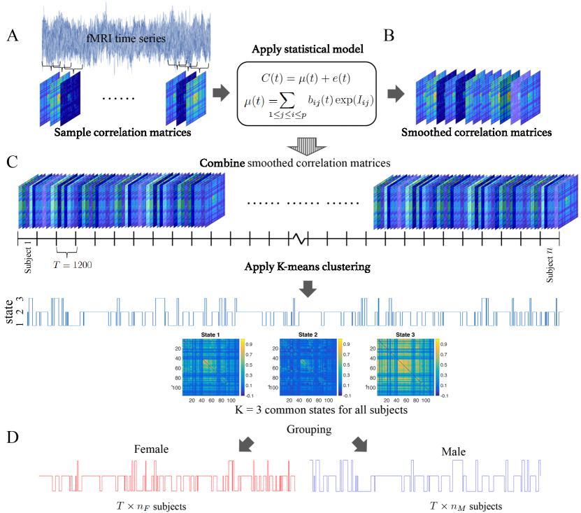
Figure 1: Schematic of estimation of dynamic connectivity states. A) For each subject, $T$ sample correlation matrices are computed by the sliding-window method. B) Original dynamic correlation matrices, composed of the $T$ sample correlation matrices, are smoothed by the proposed statistical model. C) Smoothed dynamic correlation matrices of all $n$ subjects are combined and partitioned by the $k$-means clustering to find $K$ common states. D) $T\times n$ estimated state labels are divided into male and female groups ($n_{M}$ males and $n_{F}$ females).

2.2 Clustering of the state space

The estimated dynamic functional connectivity is used in determining the state space. Assume there are $n$ subjects in the dataset. Let $C_{i}(t_{j})$ denote the $p\times p$ dynamic connectivity for the $i$-th subject at time point $t_{j}$. Let $\mathbf{d}_{j}^{i}$ denote the vectorization of the $\frac{p\times(p-1)}{2}$ elements in the upper (or lower) triangular part of matrix $C_{i}(t_{j})$. The collection of $\mathbf{d}_{j}^{i}$ over all time points and subjects is fed into the $k$-means clustering in identifying the recurring brain connectivity states that are common across subjects (Barber et al., 2018). The optimal number of cluster $K$ is determined by the elbow method which has been widely used in previous studies (Allen et al., 2014; Rashid et al., 2014; Nomi et al., 2016; Abrol et al., 2017; Lehmann et al., 2017; Barber et al., 2018; Ombao et al., 2018). Figure 1 shows the schematic of the estimation of dynamic connectivity states.

2.3 Validation

We validated the proposed method in a simulation. The MATLAB code for the simulation below can be downloaded from http://www.stat.wisc.edu/~mchung/statespaces. The simulation was independently performed 100 times, and their average is reported here. We simulated the time series of 20 subjects. The data for each subject consists of time series from $p=20$ regions, and the length of the time series is $T=300$. Then we simulated three states for each subject as follows.

The state of each subject was uniformly chosen from 1, 2 and 3 with time duration of each state randomly chosen from 5, 10, $\cdots$, 100 time points. Using this random state space as the ground truth, we simulated time series for $p=20$ regions for each subject as follows. We started with generating five $5\times 1$ data vectors ${\bf x}_{1},\cdots,{\bf x}_{5}\sim{\cal N}(0,I)$, identical and independently distributed multivariate normal with mean zero and identity matrix $I$ as the covariance. The data vector ${\bf x}_{i}$ is a noisy time series at 5 time points. Then the $5\times 1$ data vector ${\bf y}_{i}$ at region $i$ was generated with dependency as follows. We simulated ${\bf y}_{1},\cdots,{\bf y}_{4}$ identical and independently distributed multivariate normal with

$${\bf y}_{1},\cdots,{\bf y}_{4}\sim{\cal N}({\bf x}_{1},\ 0.1^{2}I).$$

Similarly we generate

$${\bf y}_{5},\cdots,{\bf y}_{8} \sim{\cal N}({\bf x}_{2},\ 0.1^{2}I)$$

$$\ \ \vdots$$

$${\bf y}_{17},\cdots,{\bf y}_{20} \sim{\cal N}({\bf x}_{5},\ 0.1^{2}I).$$

The above simulation produces modular structures in the network (Chung et al., 2017a).

Let ${\bf Y}_{1}$ be the $20\times 5$ data matrix

$${\bf Y}_{1}=[{\bf y}_{1},\cdots,{\bf y}_{20}]^{\top}.$$

Then correlation matrix $C^{1}=(c^{1}_{ij})$ corresponding to data matrix ${\bf Y}_{1}$ is given by $c^{1}_{ij}=corr({\bf y}_{i},{\bf y}_{j}).$ We repeated the above procedure twice more to obtain three independent data matrices ${\bf Y}_{1}$, ${\bf Y}_{2}$ and ${\bf Y}_{3}$ and corresponding correlation matrices $C^{1}$, $C^{2}$ and $C^{3}$ with spatial dependency between regions. The random correlation matrices with values close to each other may be difficult to discriminate. Hence, we only used ${\bf Y}_{k}$ that will give the mean squared error (MSE) between $C_{1}$, $C_{2}$ and $C_{3}$ larger than 0.5:

$$\frac{1}{20^{2}}\sum_{i,j}\left|c^{k_{1}}_{ij}-c^{k_{2}}_{ij}\right|^{2}>0.5\ \ \mbox{ for all }k_{1}\neq k_{2}.$$

We simulated the time series in $p=20$ regions for each subject as follows. If the subject is in state $k$ with time duration $5l$, the time series within this state are simulated by concatenating $20\times 5$ data matrix $Y_{k}$ repeatedly $l$ times. For instance, if the subject is in state 2 with time duration 10, state 1 with time duration 25, followed by state 3 with time duration 5, the time series were simulated as

$${\bf Y}=[{\bf Y}_{2},{\bf Y}_{2},{\bf Y}_{1},{\bf Y}_{1},{\bf Y}_{1},{\bf Y}_{1},{\bf Y}_{1},{\bf Y}_{3},\cdots],$$

where the size of whole data matrix ${\bf Y}$ is $20\times 300$ representing time series at $p=20$ regions over 300 time points. We then added noise with standard deviation $\sigma$ in the range between 0.8 and 2.4 to make each block ${\bf Y}_{k}$ slightly different from each other.

The above process is repeated 20 times for 20 subjects. We applied the sliding window method with window size 60 to obtain the original estimation of dynamic connectivity. We also applied the proposed method to smooth the dynamic connectivity. The proposed method has much less rapid state changes caused by noise (Figure 2-left), and thus has higher accuracy in state space estimation (Figure  2-right).

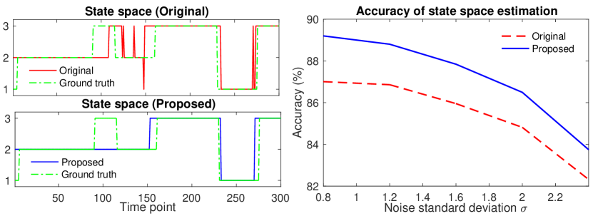
Figure 2: Left: Estimates of state space of the original and the proposed method compared to the ground truth. We only showed the results of one subject in one simulation with noise standard deviation $\sigma=2$. The proposed method has less rapid changes caused by noise. Right: Accuracy of state space estimation for $\sigma=0.8$ to $2.4$ measured by the fraction of the estimated states equal to the ground truth. The average of 100 independent simulations was plotted.

3 Application to resting-state fMRI

3.1 Dataset and preprocessing

The dataset is the resting-state fMRI of 412 subjects collected as part of the Washington University - University of Minnesota Human Connectome Project (HCP) (Van Essen et al., 2012, 2013). The resting-state fMRI were collected over 14 minutes and 33 seconds using a gradient-echo-planar imaging (EPI) sequence with multiband factor 8, time repetition (TR) 720 ms, time echo (TE) 33.1 ms, flip angle $52^{\circ}$, $104\times 90$ (RO$\times$PE) matrix size, 72 slices, 2 mm isotropic voxels, and 1200 time points. During each scanning, participants were at rest with eyes open with relaxed fixation on a projected bright cross-hair on a dark background (Van Essen et al., 2013).

The standard minimal preprocessing pipelines (Glasser et al., 2013) were applied on the fMRI scans including: spatial distortion removal (Jovicich et al., 2006; Andersson et al., 2003), motion correction (Jenkinson and Smith, 2001; Jenkinson et al., 2002), bias field reduction (Glasser and Van Essen, 2011), registration to the structural MNI template, and data masking using the brain mask obtained from FreeSurfer (Glasser et al., 2013). The resulting volumetric data contains resting-state functional time series with $91\times 109\times 91=902629$ 2-mm isotropic voxels at 1200 imaging volumes.

AAL parcellation. We employed the Automated Anatomical Labeling (AAL) template to parcellate the brain volume into 116 non-overlapping anatomical regions (Tzourio-Mazoyer et al., 2002). Spatial denoising was applied by averaging the fMRI data across voxels within each brain region, resulting in 116 average fMRI time series with 1200 time points for each subject.

Scrubbing. Previous studies reported that head movement produces spatially structured artifacts in functional connectivity (Power et al., 2012; Van Dijk et al., 2012; Satterthwaite et al., 2012; Power et al., 2015; Caballero-Gaudes and Reynolds, 2017). Thus, scrubbing was applied to remove fMRI volumes with significant head motion (Power et al., 2012). We calculated the framewise displacement (FD) from the three translational displacements ($x$, $y$, and $z$ axes) and three rotational displacements (pitch, yaw, and roll) at each time point (Power et al., 2012) to measure the head movement from one volume to the next. The first volume of each subject is assumed to have zero FD. To reduce the effect of head movement (Van Dijk et al., 2012), the volumes with FD larger than 0.5 mm and their neighbors (one back and two forward) were scrubbed (Power et al., 2012, 2013). We excluded 12 subjects having excessive head movement, and fMRI data of the remaining 400 subjects (168 males and 232 females) were used. More than one third of 1200 volumes being scrubbed in the excluded 12 subjects.

Data imputation and bandpass filtering. The imputation of the scrubbed data from the unscrubbed good data is often performed using the cubic spline interpolation in the previous studies (Allen et al., 2014; Rashid et al., 2014; Power et al., 2014; Thompson and Fransson, 2015). Further, to suppress the influence of low-frequency noise such as scanner drifts and high-frequency cardiac or respiratory oscillations (Cordes et al., 2001; van den Heuvel et al., 2008), temporal denoising by bandpass filtering is also often used (Muschelli et al., 2014; Thompson and Fransson, 2015, 2016).

In this paper, we performed data imputation and bandpass filtering together by the Fourier cosine basis (Lanczos, 1938; Hamming, 1998) with cutoff frequencies of 0.01 and 0.1 Hz (Muschelli et al., 2014; Thompson and Fransson, 2015, 2016).

3.2 Dynamic functional connectivity

For each subject, we measured the whole-brain dynamic functional connectivity by the $116\times 116$ dynamic correlation matrix computed from the average fMRI signals in the 116 brain regions using the sliding window method. Shirer et al. (2012); Leonardi and Van De Ville (2015) have reported that brain states may be correctly identified by a window size in the range of 30–60 seconds. In Allen et al. (2014), window size 44 seconds was suggested to provide a good tradeoff between the ability to resolve dynamics and quality of covariance matrix estimation. Following Allen et al. (2014), we adopted window size 60 TRs, i.e., 43.2 seconds as TR=0.72 seconds in HCP dataset. The sliding window is related to a smoother (low-pass filter) with bandwidth $1/42.3=0.0236$ Hz. To further smooth out the remaining high-frequency noise and fluctuations in the dynamic connectivity, we performed the proposed statistical model with cosine series expansion of degree 40 (corresponding to bandwidth $0.0236$ Hz). We then compared the proposed method with the original estimation of the dynamic connectivity.

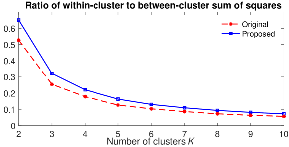
Figure 3: The ratio of within-cluster to between-cluster sum of squared distances versus the number of clusters $K=2,\cdots,10$ for the original estimation and the proposed method. By the elbow method, $K=3$ was chosen since the slope changes the most drastically at the elbow point $K=3$.

3.3 Dynamic connectivity states

The baseline $k$-means clustering was used to identify the distinct states that repetitively occur throughout the time course and are common across subjects. These discrete states serve as the basis of investigating brain connectivity. We determined the number of clusters $K$ by the elbow method which has been widely used in literature (Allen et al., 2014; Rashid et al., 2014; Nomi et al., 2016; Abrol et al., 2017; Lehmann et al., 2017; Barber et al., 2018; Ombao et al., 2018). For each value of $K$, we computed the within-cluster and between-cluster sums of squares, i.e., the sums of squared Euclidean distances between the cluster centroids and the data points within and outside the clusters. Then, we plotted the ratio of within-cluster to between-cluster sum of squares for $K=2,...,10$ (Figure 3). By the elbow method, we chose $K=3$ which gives the largest slope change in the elbow plot. Three states were also adopted by many previous studies (Choe et al., 2017; Barber et al., 2018; Ting et al., 2018b).

Figure 4: Smoothness of the dynamic correlations by the proposed statistical model. Left: The two entries of the dynamic correlation matrix of a subject. Many high-frequency fluctuations were smoothed out by the proposed model. Right: average standard deviations of the 400 subjects from averaging the standard deviations of the dynamic correlations at the 6670 brain connections. They are sorted by the average standard deviations after the proposed model. The average standard deviations became smaller after smoothing by the proposed model.

3.4 Results

Variability in each subject. There are $116\times 115/2=6670$ connections between the 116 brain regions. Figure 4-left shows the dynamic correlations of one subject at two connections. Many high-frequency fluctuations and noise in the dynamic correlations were smoothed out by the proposed statistical model. For each connection, we computed the standard deviation of the dynamic correlations over time. Then, we averaged the standard deviations across all 6670 connections. The average standard deviations of the 400 subjects are displayed in Figure 4-right.

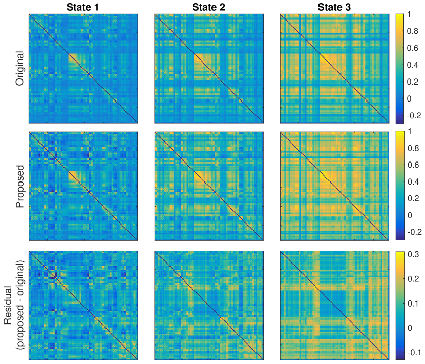
Figure 5: Top and middle: average correlation matrices (cluster centroids) of the three states for the original estimation and the proposed method. The minimum and maximum average correlations of the three states are $(-0.22,0.78)$, $(-0.06,0.88)$ and $(-0.04,0.93)$ for the original estimation, and are $(-0.34,0.88)$, $(-0.15,0.93)$ and $(-0.09,0.96)$ for the proposed method. Bottom: residual of the average correlations (proposed - original) with minimum and maximum given by $(-0.14,0.31)$, $(-0.09,0.31)$ and $(-0.05,0.31)$ in the three states.

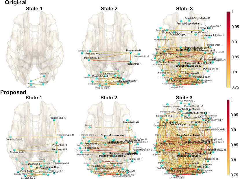
Figure 6: Average correlation matrices (cluster centroids) of the three states for the original estimation (top) and proposed method (bottom). Only connections with correlation larger than 0.75 are displayed. For both methods, the four most connected regions in states 1 and 2 are within the occipital lobe, such as the calcarine fissure and surrounding cortex, cuneus and lingual gyrus. In state 3, besides the occipital lobe, the most connected regions also include the precentral gyrus, superior temporal gyrus, and median cingulate and paracingulate gyri among other regions.

Average correlation matrix within each state. We applied the $k$-means clustering to the dynamic correlation matrices obtained from the original estimation and the proposed method. Figure 5 shows the state-specific average correlation matrices, i.e, the cluster centroids. The proposed method shows a wider range of average correlations. The minimum and maximum average correlations of the three states are $(-0.22,0.78)$, $(-0.06,0.88)$ and $(-0.04,0.93)$ for the original estimation, and are $(-0.34,0.88)$, $(-0.15,0.93)$ and $(-0.09,0.96)$ for the proposed method. The residual of the average correlations (proposed - original) ranges from $-0.14$ to $0.31$, from $-0.09$ to $0.31$, and from $-0.05$ to $0.31$ in the three states.

Figure 6 is an alternative visualization of the average correlation matrices, showing strong connections with average correlation larger than 0.75. For the original estimation and proposed method, the four most connected regions in states 1 and 2 are within the occipital lobe, such as the calcarine fissure and surrounding cortex, cuneus and lingual gyrus. In state 3, besides the occipital lobe, the most connected regions also include the precentral gyrus, superior temporal gyrus, and median cingulate and paracingulate gyri among other regions.

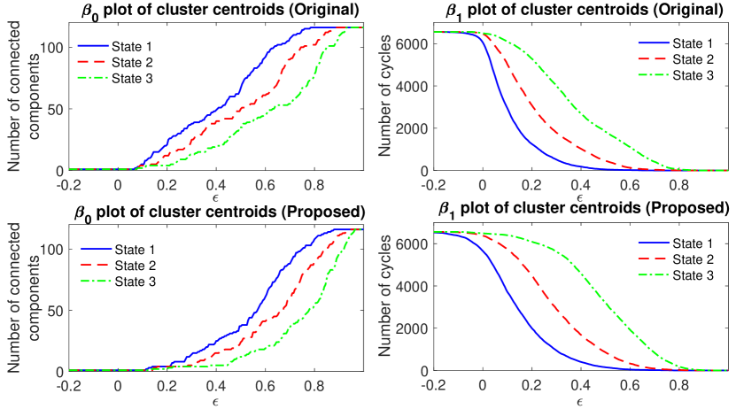
Figure 7: Betti numbers $\beta_{0}$ and $\beta_{1}$ of the brain networks thresholded by correlation value $\epsilon$. The edge weights of the networks are given by the average correlation matrices (cluster centroids) of the original estimation (top) and proposed method (bottom). The $\beta_{0}$ differences between any two states are all larger than 34 with $p$-values smaller than $9.4\times 10^{-5}$. The $\beta_{1}$ differences between any two states are all larger than 2152 with $p$-values smaller than $10^{-16}$. In both the original estimation and proposed method, the connectivity patterns of the three states are all topographically different.

Topological differences between states. We determined if the three estimated states are topologically different using the Exact Topological Inference (Chung et al., 2017b, a, 2019). We computed the 0th Betti number $\beta_{0}$ and 1st Betti number $\beta_{1}$ of the brain network in each state. We built brain networks with edge weights being the average correlations of each state. By thresholding the edge weights at higher correlation value, more edges in the networks were removed, and hence the number of connected components ($\beta_{0}$) increased while the number of cycles ($\beta_{1}$) decreased. We used threshold values ranging from $-0.2$ to 1 at an increment of 0.005. The $\beta_{0}$- and $\beta_{1}$-plots of the average correlation matrices (cluster centroids) of the three states are displayed in Figure 7. For the original estimation and proposed method, the $\beta_{0}$ differences between any two states are all larger than 34 with $p$-values smaller than $9.4\times 10^{-5}$. The $\beta_{1}$ differences between any two states are all larger than 2152 with $p$-values smaller than $10^{-16}$. The Bonferroni correction (Bonferroni, 1936; Shaffer, 1995) rejects the null hypothesis that the three states are topologically equivalent at a significance level of $\alpha=0.01$.

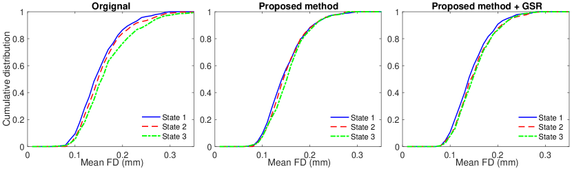
Figure 8: Cumulative distribution function of the mean framewise displacement (FD) of all subjects at each state, where the state spaces were obtained from the original estimation (left), proposed method (middle), and proposed method plus GSR (right). We compared the distributions of the three states by the Kolmogorov-Smirnov test with the Bonferroni correction. At a significance level of $\alpha=0.01$, there are state differences in the original estimation ($p=4.7\times 10^{-4}$) but no state differences in the proposed method either with or without GSR ($p=0.0326$, 0.1570).

Framewise displacement within each state. As mentioned previously, the framewise displacement (FD) was used to measure the head movement. For each subject, we computed the mean FD within each state. Figure 8 shows the distributions (cumulative distribution functions) of the mean FD of all subjects in the three states, where the state spaces were obtained from the original estimation, the proposed method, and the proposed method plus global signal regression (GSR) (Murphy et al., 2009). We performed the Kolmogorov-Smirnov test (Massey Jr., 1951) with the Bonferroni correction to compare the distributions of the three states. For the three methods, the $p$-values are $4.7\times 10^{-4}$, 0.0326 and 0.1570 respectively. Thus, at a significance level of $\alpha=0.01$, there are state differences in head movement in the original estimation but no state differences in head movement in the proposed method with or without GSR. Thus, GSR was not used in this study.

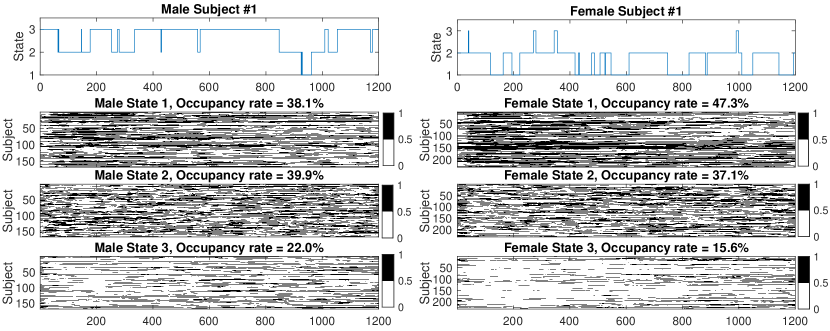
(a)

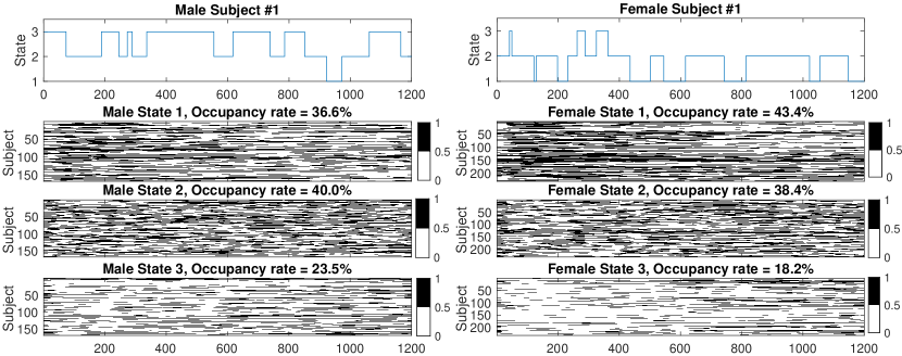
(b)

Figure 9: In the (a) original estimation and (b) proposed method, the first row shows the dynamic connectivity states of the 1st male (left) and 1st female (right) subjects. The proposed method has less rapid changes in the dynamic connectivity states. The 2nd to 4th rows are the plots of he state occupancy of all the 168 males (left) and 232 females (right). Correlation matrices belonging to the state are marked by black.

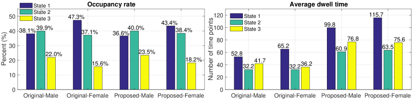
Figure 10: Left: Occupancy rates of the three states, i.e., the percentage of the entire scan time that a male/female spends in each state. On average, males spent more time in state 2 while females spent more time in state 1. Right: Average dwell time of the three states, i.e., the average period of time a male/female remains in a given state before switching to another state. On average, a subject dwelt in state 1 for a longer period, and females had longer dwell time in state 1 than males. The proposed method has longer average dwell time than the original estimation due to less rapid state changes.

Occupancy rate and dwell time. To analyze the difference between males and females in dynamic connectivity states, we further divided the clustering results into male and female groups (168 males and 232 females). Figure 9 shows the dynamic connectivity states of the 1st male and 1st female subjects as an example. The proposed method has less number of rapid changes in the dynamic connectivity states. Figure 9 also shows the occupancy of the three states for all male and female subjects. Let $s_{ij}\in\{1,2,3\}$ denote the state of subject $i$ at time point $t_{j}$ estimated by the $k$-means clustering. The occupancy rate (Yaesoubi et al., 2015; Ombao et al., 2018) of state $k$ is computed as

$$\frac{1}{nT}\sum_{i=1}^{n}\sum_{j=1}^{T}\left(s_{ij}=k\right),$$

where $T=1200$ time points and $n=168$ and 232 subjects for male and female groups respectively. On average, males spent more time in state 2, while females spent more time in state 1 (Figure 10-left).

We also computed the dwell time (Damaraju et al., 2014; Lottman et al., 2017; Barber et al., 2018), i.e., the period of time a male/female remains in a given state before switching to another state. The average dwell time for males and females in each state is displayed in Figure 10-right. On average, a subject dwelt in state 1 for a longer period, and females had longer dwell time in state 1 than males. The proposed method shows longer average dwell time than the original estimation due to less rapid state changes.

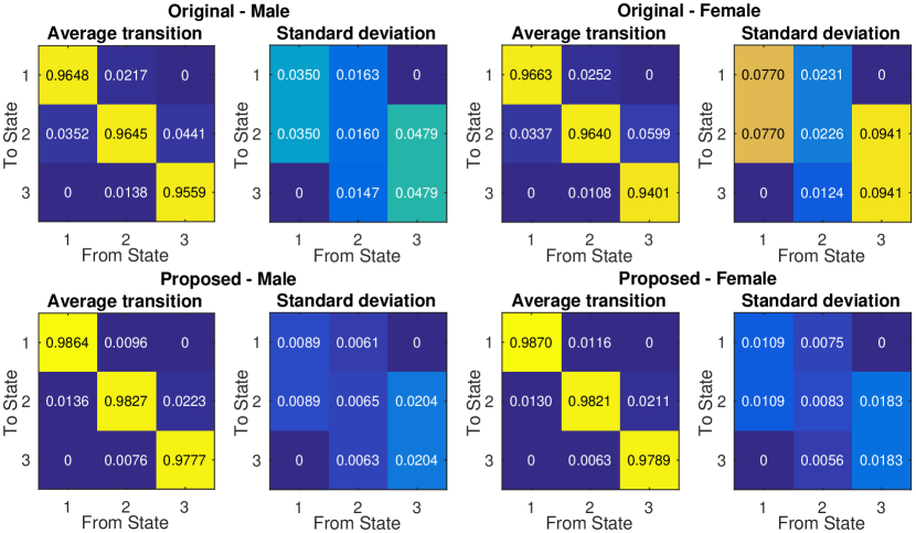
Figure 11: Averages and standard deviations of transition probabilities of males (left) and females (right) computed from the dynamic connectivity states of the original estimation (top) and the proposed method (bottom). The proposed method reduced the transition probabilities between different states and increased the probabilities of remaining in the same state.

Transition probability. We used state transitions to reveal the interactions between different brain states (Baker et al., 2014). They can be modeled as a Markov chain (Gilks et al., 1995). For subject $i$, the transition probability of moving from state $k_{1}$ to state $k_{2}$ is computed by

$$P\left(s_{ij}=k_{2}|\ s_{i,j-1}=k_{1}\right),$$

where $s_{ij}$ is the state of subject $i$ at time point $t_{j}$ estimated by the $k$-means clustering. Figure 11 shows the averages and standard deviations of the transition probabilities of males and females. Each subject remained in the same state for a long period of time before transitioning to other state. The proposed method reduced the transition probabilities between different states and increased the probabilities of remaining in the same state because some transitions caused by noise were removed. The very low average transition probabilities between state 1 and state 3 show the inability of transitioning directly between these two states.

Statistical analysis. To compare males and females in state transition probability, comparison of mean sample proportions was utilized. Consider the null hypothesis that the averages of estimated transition probabilities from state $k_{1}$ to $k_{2}$ for males and females are the same. The z-score was computed from

$$Z=\frac{\bar{P}_{M}-\bar{P}_{F}}{\sqrt{\frac{\sigma^{2}_{M}}{n_{M}}+\frac{\sigma^{2}_{F}}{n_{F}}}},$$

where $\overline{P}_{M}$ and $\overline{P}_{F}$ are the means of the transition probabilities for $n_{M}$ males and $n_{F}$ females respectively, and $\sigma^{2}_{M}$ and $\sigma^{2}_{F}$ are the variances of the transition probabilities. The z-scores and the corresponding $p$-values are shown in Figure 12. In the original estimation, there is significant difference at $p$-values $<0.05$ in the transition probability from state 2 to state 3 ($2\rightarrow 3$). In the proposed method, there are significant differences at $p$-values $<0.05$ in the transition probabilities of ($2\rightarrow 1$) and ($2\rightarrow 3$).

We further tested the statistical significance of state occupancy rates between females and males, by setting the null hypothesis that males and females have the same mean of occupancy rate. The $p$-values of the z-test are shown in Table 1. For both the original estimation and proposed method, there are differences in the occupancy rates of states 1 and 3 at significance level 0.05.

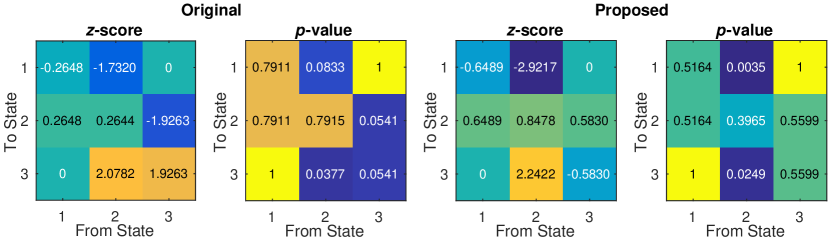
Figure 12: Z-test for differences in transition probabilities between males and females using the difference in the mean proportions at significance level 0.05. In the original estimation (left), there is significant difference in the transition probability of ($2\rightarrow 3$). In the proposed method (right), there are significant differences in the transition probabilities of ($2\rightarrow 1$) and ($2\rightarrow 3$).

Table 1: $p$-values of the z-test for gender differences in state occupancy rates.

State	Original	Proposed
1	$0.0019$	$0.0114$
2	$0.1445$	$0.3685$
3	$0.0050$	$0.0215$

4 Discussions

Dynamic connectivity. In this study, we found that the average correlation matrices (cluster centroids) of the three states followed similar connectivity patterns of the previous study (Haimovici et al., 2017), which also used the AAL parcellation but $k$-means clustering with four states. In Haimovici et al. (2017), two of the four states show high average correlation in many brain connections. In our result, the three states are not disjoint but share similar connectivity pattern. This may be due to the small number of clusters, which can also be observed in Cai et al. (2018). Consider the resting state networks (Ting et al., 2018a; Al-sharoa et al., 2019). The average correlation matrices of the three states show relative higher correlations in the occipital lobe, such as calcarine fissure and surrounding cortex, cuneus and lingual gyrus. Compared to other resting state networks, the visual network has the strongest connectivity across different states, followed by the somatomotor network including brain regions such as the postcentral gyrus and precentral gyrus.

Transition probability of brain state. The resting-state networks tend to remain in the same state for a long period before switching to another state (Allen et al., 2014; Shakil et al., 2016; Calhoun and Adali, 2016; Abrol et al., 2017; Nielsen et al., 2018). In this study, we showed that the state space of the proposed method had a longer stability (less rapid changes and longer dwell time) and a higher probability of remaining in the same state compared to the original estimation.

Estimation of dynamic functional connectivity. The proposed model aims for smoothing out unwanted high-frequency fluctuations in the original estimation of dynamic connectivity which may introduce rapid changes in brain state estimation in resting state. There are a variety of dynamic connectivity estimation methods besides the sliding window method, such as the tapered sliding window (Allen et al., 2014; Lindquist et al., 2014; Abrol et al., 2017), flexible least squares (Liao et al., 2014), multiplication of temporal derivatives (Shine et al., 2015), and jackknife correlation (Thompson et al., 2018; Thompson and Fransson, 2018). It is still unclear which method is the optimal since the true dynamic connectivity is unknown. For instance, Thompson et al. (2018) showed in simulations that the jackknife correlation outperforms the sliding and tapered sliding window methods when the state changes quickly, but the taped sliding window method followed sliding window method performs the best when the state changes slowly. In this paper, we used the sliding window method as it may be the simplest and most widely used method, but the proposed model can be applied to other estimation methods. The performance of the proposed model would vary depending on the original estimation of the dynamic connectivity.

Smoothing of dynamic functional connectivity. The proposed model contains a temporal smoothing, which fits the time-varying coefficients to a cosine series representation and estimates the cosine series coefficients by the least squares method (Chung et al., 2010). Other least squares smoothing methods can be applied instead, but the smoothing result might be different. For example, the least squares smoothing in Selesnick et al. (2012); Baek et al. (2015) minimizes the second-order difference to force the signal to be smooth. The Savitzky–Golay Filter (Savitzky and Golay, 1964; Madden, 1978) fits the subsets of adjacent data points to a polynomial by linear least squares. This is left as a future study.

5 Conclusion

In the proposed regression method, the dynamic correlation matrix is modeled as a linear combination of symmetric positive-definite (SPD) matrices combined with cosine series representation, which provides superior performance over existing sample correlation matrices. We represented the correlation matrix, at each time point, as a linear combination of exponential map of the orthonormal basis in the space of symmetric matrices. Doing so, we smoothed out the unwanted noise in dynamic functional connectivity and achieved higher accuracy in identifying and discriminating brain connectivity states.

References

References

- Abrol et al. (2017) Abrol, A., Damaraju, E., Miller, R.L., Stephen, J.M., Claus, E.D., Mayer, A.R., Calhoun, V.D., 2017. Replicability of time-varying connectivity patterns in large resting state fMRI samples. NeuroImage 163, 160–176.
- Al-sharoa et al. (2019) Al-sharoa, E., Al-khassaweneh, M., Aviyente, S., 2019. Tensor based temporal and multilayer community detection for studying brain dynamics during resting state fMRI. IEEE Transactions on Biomedical Engineering 66, 695–709.
- Allen et al. (2014) Allen, E.A., Damaraju, E., Plis, S.M., Erhardt, E.B., Eichele, T., Calhoun, V.D., 2014. Tracking whole-brain connectivity dynamics in the resting state. Cerebral Cortex 24, 663–676.
- Andersson et al. (2003) Andersson, J.L.R., Skare, S., Ashburner, J., 2003. How to correct susceptibility distortions in spin-echo echo-planar images: application to diffusion tensor imaging. NeuroImage 20, 870–888.
- Arsigny et al. (2006) Arsigny, V., Fillard, P., Pennec, X., Ayache, N., 2006. Log-Euclidean metrics for fast and simple calculus on diffusion tensors. Magnetic Resonance in Medicine 56, 411–421.
- Arsigny et al. (2007) Arsigny, V., Fillard, P., Pennec, X., Ayache, N., 2007. Geometric means in a novel vector space structure on symmetric positive-definite matrices. SIAM Journal on Matrix Analysis and Applications 29, 328–347.
- Baek et al. (2015) Baek, S.J., Park, A., Ahn, Y.J., Choo, J., 2015. Baseline correction using asymmetrically reweighted penalized least squares smoothing. Analyst 140, 250–257.
- Baker et al. (2014) Baker, A.P., Brookes, M.J., Rezek, I.A., Smith, S.M., Behrens, T., Smith, P.J.P., Woolrich, M., 2014. Fast transient networks in spontaneous human brain activity. Elife 3, e01867.
- Barber et al. (2018) Barber, A.D., Lindquist, M.A., DeRosse, P., Karlsgodt, K.H., 2018. Dynamic functional connectivity states reflecting psychotic-like experiences. Biological Psychiatry 3, 443–453.
- Barmpoutis et al. (2007) Barmpoutis, A., Vemuri, B.C., Shepherd, T.M., Forder, J.R., 2007. Tensor splines for interpolation and approximation of DT-MRI with applications to segmentation of isolated rat hippocampi. IEEE Transactions on Medical Imaging 26, 1537–1546.
- Barttfeld et al. (2015) Barttfeld, P., Uhrig, L., Sitt, J.D., Sigman, M., Jarraya, B., Dehaene, S., 2015. Signature of consciousness in the dynamics of resting-state brain activity. Proceedings of the National Academy of Sciences 112, 887–892.
- Bonferroni (1936) Bonferroni, C., 1936. Teoria statistica delle classi e calcolo delle probabilita. Pubblicazioni del R Istituto Superiore di Scienze Economiche e Commericiali di Firenze 8, 3–62.
- Caballero-Gaudes and Reynolds (2017) Caballero-Gaudes, C., Reynolds, R.C., 2017. Methods for cleaning the BOLD fMRI signal. NeuroImage 154, 128–149.
- Cai et al. (2018) Cai, B., Zille, P., Stephen, J.M., Wilson, T.W., Calhoun, V.D., Wang, Y.P., 2018. Estimation of dynamic sparse connectivity patterns from resting state fMRI. IEEE Transactions on Medical Imaging 37, 1224–1234.
- Calhoun and Adali (2016) Calhoun, V.D., Adali, T., 2016. Time-varying brain connectivity in fMRI data: whole-brain data-driven approaches for capturing and characterizing dynamic states. IEEE Signal Processing Magazine 33, 52–66.
- Calhoun et al. (2014) Calhoun, V.D., Miller, R., Pearlson, G., Adalı, T., 2014. The chronnectome: time-varying connectivity networks as the next frontier in fMRI data discovery. Neuron 84, 262–274.
- Chang and Glover (2010) Chang, C., Glover, G.H., 2010. Time–frequency dynamics of resting-state brain connectivity measured with fMRI. NeuroImage 50, 81–98.
- Cheng et al. (2012) Cheng, G., Salehian, H., Vemuri, B.C., 2012. Efficient recursive algorithms for computing the mean diffusion tensor and applications to DTI segmentation. In: European Conference on Computer Vision. Lecture Notes in Computer Science 7578, 390–401.
- Choe et al. (2017) Choe, A.S., Nebel, M.B., Barber, A.D., Cohen, J.R., Xu, Y., Pekar, J.J., Caffo, B., Lindquist, M.A., 2017. Comparing test-retest reliability of dynamic functional connectivity methods. NeuroImage 158, 155–175.
- Chung et al. (2010) Chung, M.K., Adluru, N., Lee, J.E., Lazar, M., Lainhart, J.E., Alexander, A.L., 2010. Cosine series representation of 3D curves and its application to white matter fiber bundles in diffusion tensor imaging. Statistics and Its Interface 3, 69–80.
- Chung et al. (2019) Chung, M.K., Huang, S.G., Gritsenko, A., Shen, L., Lee, H., 2019. Statistical inference on the number of cycles in brain networks, in: IEEE 16th International Symposium on Biomedical Imaging, pp. 113–116.
- Chung et al. (2017a) Chung, M.K., Lee, H., Solo, V., Davidson, R.J., Pollak, S.D., 2017a. Topological distances between brain networks. In: International Workshop on Connectomics in Neuroimaging. Lecture Notes in Computer Science 10511, 161–170.
- Chung et al. (2017b) Chung, M.K., Villalta-Gil, V., Lee, H., Rathouz, P.J., Lahey, B.B., Zald, D.H., 2017b. Exact topological inference for paired brain networks via persistent homology. In: Information Processing in Medical Imaging. Lecture Notes in Computer Science 10265, 299–310.
- Cordes et al. (2001) Cordes, D., Haughton, V.M., Arfanakis, K., Carew, J.D., Turski, P.A., Moritz, C.H., Quigley, M.A., Meyerand, M.E., 2001. Frequencies contributing to functional connectivity in the cerebral cortex in “resting-state” data. American Journal of Neuroradiology 22, 1326–1333.
- Damaraju et al. (2014) Damaraju, E., Allen, E.A., Belger, A., Ford, J.M., McEwen, S., Mathalon, D.H., Mueller, B.A., Pearlson, G.D., Potkin, S.G., Preda, A., et al., 2014. Dynamic functional connectivity analysis reveals transient states of dysconnectivity in schizophrenia. NeuroImage: Clinical 5, 298–308.
- Fillard et al. (2007) Fillard, P., Pennec, X., Arsigny, V., Ayache, N., 2007. Clinical DT-MRI estimation, smoothing, and fiber tracking with log-Euclidean metrics. IEEETransactions on Medical Imaging 26, 1472–1482.
- Fletcher (2013) Fletcher, P.T., 2013. Geodesic regression and the theory of least squares on Riemannian manifolds. International Journal of Computer Vision 105, 171–185.
- Gilks et al. (1995) Gilks, W.R., Richardson, S., Spiegelhalter, D., 1995. Markov chain Monte Carlo in practice. Chapman and Hall/CRC.
- Glasser et al. (2013) Glasser, M.F., Sotiropoulos, S.N., Wilson, J.A., Coalson, T.S., Fischl, B., Andersson, J.L., Xu, J., Jbabdi, S., Webster, M., Polimeni, J.R., et al., 2013. The minimal preprocessing pipelines for the Human Connectome Project. NeuroImage 80, 105–124.
- Glasser and Van Essen (2011) Glasser, M.F., Van Essen, D.C., 2011. Mapping human cortical areas in vivo based on myelin content as revealed by T1-and T2-weighted MRI. Journal of Neuroscience 31, 11597–11616.
- Haimovici et al. (2017) Haimovici, A., Tagliazucchi, E., Balenzuela, P., Laufs, H., 2017. On wakefulness fluctuations as a source of BOLD functional connectivity dynamics. Scientific Reports 7, 5908.
- Hall (2015) Hall, B., 2015. Lie groups, Lie algebras, and representations: an elementary introduction. volume 222. Springer.
- Hamming (1998) Hamming, R.W., 1998. Digital filters. Courier Corporation.
- van den Heuvel et al. (2008) van den Heuvel, M.P., Stam, C.J., Boersma, M., Hulshoff Pol, H.E., 2008. Small-world and scale-free organization of voxel-based resting-state functional connectivity in the human brain. NeuroImage 43, 528–539.
- Hindriks et al. (2016) Hindriks, R., Adhikari, M.H., Murayama, Y., Ganzetti, M., Mantini, D., Logothetis, N.K., Deco, G., 2016. Can sliding-window correlations reveal dynamic functional connectivity in resting-state fMRI? NeuroImage 127, 242–256.
- Hinkle et al. (2014) Hinkle, J., Fletcher, P.T., Joshi, S., 2014. Intrinsic polynomials for regression on Riemannian manifolds. Journal of Mathematical Imaging and Vision 50, 32–52.
- Hutchison and Morton (2015) Hutchison, R.M., Morton, J.B., 2015. Tracking the brain’s functional coupling dynamics over development. Journal of Neuroscience 35, 6849–6859.
- Hutchison et al. (2013) Hutchison, R.M., Womelsdorf, T., Allen, E.A., Bandettini, P.A., Calhoun, V.D., Corbetta, M., Della Penna, S., Duyn, J.H., Glover, G.H., Gonzalez-Castillo, J., et al., 2013. Dynamic functional connectivity: Promise, issues, and interpretations. NeuroImage 80, 360–378.
- Jenkinson et al. (2002) Jenkinson, M., Bannister, P., Brady, M., Smith, S., 2002. Improved optimization for the robust and accurate linear registration and motion correction of brain images. NeuroImage 17, 825–841.
- Jenkinson and Smith (2001) Jenkinson, M., Smith, S., 2001. A global optimisation method for robust affine registration of brain images. Medical Image Analysis 5, 143–156.
- Jovicich et al. (2006) Jovicich, J., Czanner, S., Greve, D., Haley, E., van Der Kouwe, A., Gollub, R., Kennedy, D., Schmitt, F., Brown, G., MacFall, J., et al., 2006. Reliability in multi-site structural MRI studies: effects of gradient non-linearity correction on phantom and human data. NeuroImage 30, 436–443.
- Keilholz et al. (2013) Keilholz, S.D., Magnuson, M.E., Pan, W.J., Willis, M., Thompson, G.J., 2013. Dynamic properties of functional connectivity in the rodent. Brain Connectivity 3, 31–40.
- Kim et al. (2017) Kim, H.J., Adluru, N., Suri, H., Vemuri, B.C., Johnson, S.C., Singh, V., 2017. Riemannian nonlinear mixed effects models: Analyzing longitudinal deformations in neuroimaging, in: IEEE Conference on Computer Vision and Pattern Recognition, pp. 2540–2549.
- Kucyi and Davis (2014) Kucyi, A., Davis, K.D., 2014. Dynamic functional connectivity of the default mode network tracks daydreaming. NeuroImage 100, 471–480.
- Lanczos (1938) Lanczos, C., 1938. Trigonometric interpolation of empirical and analytical functions. Journal of Mathematics and Physics 17, 123–199.
- Lehmann et al. (2017) Lehmann, B.C.L., White, S.R., Henson, R.N., Cam-CAN, Geerligs, L., 2017. Assessing dynamic functional connectivity in heterogeneous samples. NeuroImage 157, 635–647.
- Leonardi and Van De Ville (2015) Leonardi, N., Van De Ville, D., 2015. On spurious and real fluctuations of dynamic functional connectivity during rest. NeuroImage 104, 430–436.
- Liao et al. (2014) Liao, W., Wu, G.R., Xu, Q., Ji, G.J., Zhang, Z., Zang, Y.F., Lu, G., 2014. DynamicBC: a MATLAB toolbox for dynamic brain connectome analysis. Brain Connectivity 4, 780–790.
- Lindquist et al. (2014) Lindquist, M.A., Xu, Y., Nebel, M.B., Caffo, B.S., 2014. Evaluating dynamic bivariate correlations in resting-state fMRI: a comparison study and a new approach. NeuroImage 101, 531–546.
- Lottman et al. (2017) Lottman, K.K., Kraguljac, N.V., White, D.M., Morgan, C.J., Calhoun, V.D., Butt, A., Lahti, A.C., 2017. Risperidone effects on brain dynamic connectivity–a prospective resting state fMRI study in schizophrenia. Frontiers in Psychiatry 8, 14.
- Lurie et al. (2018) Lurie, D., Kessler, D., Bassett, D., Betzel, R.F., Breakspear, M., Keilholz, S., Kucyi, A., Liégeois, R., Lindquist, M.A., McIntosh, A.R., et al., 2018. On the nature of time-varying functional connectivity in resting fMRI. URL: psyarxiv.com/xtzre.
- Madden (1978) Madden, H.H., 1978. Comments on the Savitzky-Golay convolution method for least-squares-fit smoothing and differentiation of digital data. Analytical Chemistry 50, 1383–1386.
- Marusak et al. (2017) Marusak, H.A., Calhoun, V.D., Brown, S., Crespo, L.M., Sala-Hamrick, K., Gotlib, I.H., Thomason, M.E., 2017. Dynamic functional connectivity of neurocognitive networks in children. Human Brain Mapping 38, 97–108.
- Massey Jr. (1951) Massey Jr., F.J., 1951. The Kolmogorov-Smirnov test for goodness of fit. Journal of the American statistical Association 46, 68–78.
- Moakher and Batchelor (2006) Moakher, M., Batchelor, P.G., 2006. Symmetric positive-definite matrices: From geometry to applications and visualization, in: Visualization and Processing of Tensor Fields. Springer, pp. 285–298.
- Murphy et al. (2009) Murphy, K., Birn, R.M., Handwerker, D.A., Jones, T.B., Bandettini, P.A., 2009. The impact of global signal regression on resting state correlations: Are anti-correlated networks introduced? NeuroImage 44, 893–905.
- Muschelli et al. (2014) Muschelli, J., Nebel, M.B., Caffo, B.S., Barber, A.D., Pekar, J.J., Mostofsky, S.H., 2014. Reduction of motion-related artifacts in resting state fMRI using aCompCor. NeuroImage 96, 22–35.
- Nielsen et al. (2018) Nielsen, S.F.V., Schmidt, M.N., Madsen, K.H., Mørup, M., 2018. Predictive assessment of models for dynamic functional connectivity. NeuroImage 171, 116–134.
- Nomi et al. (2016) Nomi, J.S., Farrant, K., Damaraju, E., Rachakonda, S., Calhoun, V.D., Uddin, L.Q., 2016. Dynamic functional network connectivity reveals unique and overlapping profiles of insula subdivisions. Human Brain Mapping 37, 1770–1787.
- Ombao et al. (2018) Ombao, H., Fiecas, M., Ting, C.M., Low, Y.F., 2018. Statistical models for brain signals with properties that evolve across trials. NeuroImage 180, 609–618.
- Power et al. (2012) Power, J.D., Barnes, K.A., Snyder, A.Z., Schlaggar, B.L., Petersen, S.E., 2012. Spurious but systematic correlations in functional connectivity MRI networks arise from subject motion. NeuroImage 59, 2142–2154.
- Power et al. (2013) Power, J.D., Barnes, K.A., Snyder, A.Z., Schlaggar, B.L., Petersen, S.E., 2013. Steps toward optimizing motion artifact removal in functional connectivity MRI; a reply to carp. NeuroImage 76.
- Power et al. (2014) Power, J.D., Mitra, A., Laumann, T.O., Snyder, A.Z., Schlaggar, B.L., Petersen, S.E., 2014. Methods to detect, characterize, and remove motion artifact in resting state fMRI. NeuroImage 84, 320–341.
- Power et al. (2015) Power, J.D., Schlaggar, B.L., Petersen, S.E., 2015. Recent progress and outstanding issues in motion correction in resting state fMRI. NeuroImage 105, 536–551.
- Preti et al. (2017) Preti, M.G., Bolton, T.A., Van De Ville, D., 2017. The dynamic functional connectome: State-of-the-art and perspectives. NeuroImage 160, 41–54.
- Qiu et al. (2015) Qiu, A., Lee, A., Tan, M., Chung, M.K., 2015. Manifold learning on brain functional networks in aging. Medical image analysis 20, 52–60.
- Rashid et al. (2016) Rashid, B., Arbabshirani, M.R., Damaraju, E., Cetin, M.S., Miller, R., Pearlson, G.D., Calhoun, V.D., 2016. Classification of schizophrenia and bipolar patients using static and dynamic resting-state fMRI brain connectivity. NeuroImage 134, 645–657.
- Rashid et al. (2014) Rashid, B., Damaraju, E., Pearlson, G.D., Calhoun, V.D., 2014. Dynamic connectivity states estimated from resting fMRI identify differences among schizophrenia, bipolar disorder, and healthy control subjects. Frontiers in Human Neuroscience 8, 897.
- Samdin et al. (2017) Samdin, S.B., Ting, C.M., Ombao, H., Salleh, S.H., 2017. A unified estimation framework for state-related changes in effective brain connectivity. IEEE Transactions on Biomedical Engineering 64, 844–858.
- Satterthwaite et al. (2012) Satterthwaite, T.D., Wolf, D.H., Loughead, J., Ruparel, K., Elliott, M.A., Hakonarson, H., Gur, R.C., Gur, R.E., 2012. Impact of in-scanner head motion on multiple measures of functional connectivity: Relevance for studies of neurodevelopment in youth. NeuroImage 60, 623–632.
- Savitzky and Golay (1964) Savitzky, A., Golay, M.J.E., 1964. Smoothing and differentiation of data by simplified least squares procedures. Analytical Chemistry 36, 1627–1639.
- Selesnick et al. (2012) Selesnick, I.W., Arnold, S., Dantham, V.R., 2012. Polynomial smoothing of time series with additive step discontinuities. IEEE Transactions on Signal Processing 60, 6305–6318.
- Shaffer (1995) Shaffer, J.P., 1995. Multiple hypothesis testing. Annual Review of Psychology 46, 561–584.
- Shakil et al. (2016) Shakil, S., Lee, C.H., Keilholz, S.D., 2016. Evaluation of sliding window correlation performance for characterizing dynamic functional connectivity and brain states. NeuroImage 133, 111–128.
- Shine et al. (2015) Shine, J.M., Koyejo, O., Bell, P.T., Gorgolewski, K.J., Gilat, M., Poldrack, R.A., 2015. Estimation of dynamic functional connectivity using multiplication of temporal derivatives. NeuroImage 122, 399–407.
- Shirer et al. (2012) Shirer, W.R., Ryali, S., Rykhlevskaia, E., Menon, V., Greicius, M.D., 2012. Decoding subject-driven cognitive states with whole-brain connectivity patterns. Cerebral Cortex 22, 158–165.
- Su et al. (2016) Su, J., Shen, H., Zeng, L.L., Qin, J., Liu, Z., Hu, D., 2016. Heredity characteristics of schizophrenia shown by dynamic functional connectivity analysis of resting-state functional MRI scans of unaffected siblings. NeuroReport 27, 843–848.
- Thompson and Fransson (2015) Thompson, W.H., Fransson, P., 2015. The frequency dimension of fMRI dynamic connectivity: Network connectivity, functional hubs and integration in the resting brain. NeuroImage 121, 227–242.
- Thompson and Fransson (2016) Thompson, W.H., Fransson, P., 2016. Bursty properties revealed in large-scale brain networks with a point-based method for dynamic functional connectivity. Scientific Reports 6, 39156.
- Thompson and Fransson (2018) Thompson, W.H., Fransson, P., 2018. A common framework for the problem of deriving estimates of dynamic functional brain connectivity. NeuroImage 172, 896–902.
- Thompson et al. (2018) Thompson, W.H., Richter, C.G., Plavén-Sigray, P., Fransson, P., 2018. Simulations to benchmark time-varying connectivity methods for fMRI. PLoS Computational Biology 14, e1006196.
- Ting et al. (2018a) Ting, C.M., Ombao, H., Salleh, S.H., Abd Latif, A.Z., 2018a. Multi-scale factor analysis of high-dimensional functional connectivity in brain networks. IEEE Transactions on Network Science and Engineering. doi:10.1109/TNSE.2018.2869862.
- Ting et al. (2018b) Ting, C.M., Ombao, H., Samdin, S.B., Salleh, S.H., 2018b. Estimating dynamic connectivity states in fMRI using regime-switching factor models. IEEE Transactions on Medical Imaging 37, 1011–1023.
- Tzourio-Mazoyer et al. (2002) Tzourio-Mazoyer, N., Landeau, B., Papathanassiou, D., Crivello, F., Etard, O., Delcroix, N., Mazoyer, B., Joliot, M., 2002. Automated anatomical labeling of activations in SPM using a macroscopic anatomical parcellation of the MNI MRI single-subject brain. NeuroImage 15, 273–289.
- Van Dijk et al. (2012) Van Dijk, K.R.A., Sabuncu, M.R., Buckner, R.L., 2012. The influence of head motion on intrinsic functional connectivity MRI. NeuroImage 59, 431–438.
- Van Essen et al. (2013) Van Essen, D.C., Smith, S.M., Barch, D.M., Behrens, T.E.J., Yacoub, E., Ugurbil, K., 2013. The WU-Minn Human Connectome Project: An overview. NeuroImage 80, 62–79.
- Van Essen et al. (2012) Van Essen, D.C., Ugurbil, K., Auerbach, E., Barch, D., Behrens, T.E.J., Bucholz, R., Chang, A., Chen, L., Corbetta, M., Curtiss, S.W., et al., 2012. The Human Connectome Project: A data acquisition perspective. Neuroimage 62, 2222–2231.
- Wong et al. (2018) Wong, E., Anderson, J.S., Zielinski, B.A., Fletcher, P.T., 2018. Riemannian regression and classification models of brain networks applied to autism. In: International Workshop on Connectomics in Neuroimaging. Lecture Notes in Computer Science 11083, 78–87.
- Yaesoubi et al. (2015) Yaesoubi, M., Allen, E.A., Miller, R.L., Calhoun, V.D., 2015. Dynamic coherence analysis of resting fMRI data to jointly capture state-based phase, frequency, and time-domain information. NeuroImage 120, 133–142.
- Yang et al. (2014) Yang, Z., Craddock, R.C., Margulies, D.S., Yan, C.G., Milham, M.P., 2014. Common intrinsic connectivity states among posteromedial cortex subdivisions: Insights from analysis of temporal dynamics. NeuroImage 93, 124–137.
- Zalesky and Breakspear (2015) Zalesky, A., Breakspear, M., 2015. Towards a statistical test for functional connectivity dynamics. NeuroImage 114, 466–470.