Theory of Shear Modulus in Glasses

Abstract

We construct a linear response theory of applying shear deformations from boundary walls in the film geometry in Kubo’s theoretical scheme. Our method is applicable to any solids and fluids. For glasses, we assume quasi-equilibrium around a fixed inherent state. Then, we obtain linear-response expressions for any variables including the stress and the particle displacements, even though the glass interior is elastically inhomogeneous. In particular, the shear modulus can be expressed in terms of the correlations between the interior stress and the forces from the walls. It can also be expressed in terms of the inter-particle correlations, as has been shown in the previous literature. Our stress relaxation function includes the effect of the boundary walls and can be used for inhomogeneous flow response. We show the presence of long-ranged, long-lived correlations among the fluctuations of the forces from the walls and the displacements of all the particles in the cell. We confirm these theoretical results numerically in a two-dimensional model glass. As an application, we describe propagation of transverse sounds after boundary wall motions using these time-correlation functions We also find resonant sound amplification when the frequency of an oscillatory shear approaches that of the first transverse sound mode.

I Introduction

In glasses, the structural relaxation becomes exceedingly slow at low temperature $T$. The shear modulus $\mu$ is then well-defined for small deformations, though plastic events easily take place with increasing the applied strainLiu ; Lacks ; Maeda ; Yama1 ; Kawasaki ; Malo2 ; Barr3 . It is of great interest how $\mu$ in glasses depends on the disordered particle configuration. On the other hand, in crystals, the microscopic expressions for the elastic moduli can be derived under a homogeneously applied strain (or stress) in equilibriumHoover ; Ray ; Lutsko ; Pablo ; Hess . Such expressions are composed of a positive affine part and a negative nonaffine part, where the latter arises from the correlation of the stress fluctuations. If the moduli are homogeneous, they can be related to the variances of the thermal strain (or stress) fluctuations divided by $k_{B}T$Rahman ; Binder ; Gusev .

In glasses, $\mu$ is expressed in the same form as those in crystals in terms of the particle positions on timescales without plastic eventsMalo ; Malo1 ; Evans ; Wil ; Yoshi ; Ilg ; Barr1 ; Barr2 ; Saw ; Wit ; Wit1 ; Teren ; Za . To derive this expression, Maloney and LemaîtreMalo ; Malo1 examined the local minima of the potential energy under constraint of a fixed mean strain in the periodic boundary condition. Remarkably, the local values of $\mu$ exhibit mesoscopic inhomogeneityPabloP ; Miz1 . In fact, in glasses, the displacements (and suitably defined strains) in glasses are highly heterogeneous on mesoscopic scales under shearBarr1 ; Barr2 ; Malo2 ; Yama1 ; Kawasaki ; Liu ; Maeda ; Barr3 .

The linear response theory in statistical mechanics has a long historyHansen ; Onukibook ; Zwan . On the basis of Onsager’s theoryOnsager , GreenGreen derived time-evolution equations for gross variables, which was rigorously justified by ZwanzigZwan . Green then expressed the transport coefficients in fluids such as the viscosities and the thermal conductivity in terms of the time-correlation functions of the stress and the heat flux, respectively. These expressions also followed from the relaxation behaviors of the time-correlation functions of hydrodynamic variablesHansen ; Kada ; Zwan . KuboKubo studied linear response to mechanical forces, for which the Hamiltonian consists of the unperturbed one $\cal H$ and a small time-dependent perturbation as

$${\cal H}^{\prime}={\cal H}-\gamma_{\rm ex}(t){\cal A}.$$ (1)

Here, $\gamma_{\rm ex}(t)$ is an applied force and ${\cal A}$ is its conjugate variable. Thus, there was a conceptual difference between the approaches to thermal and mechanical disturbances.

In this paper, we set up a Hamiltonian in the form of Eq.(1) for slight motions of the boundary walls in the film geometry, where the film thickness $H$ is much longer than the particle sizes. Here, $\gamma_{\rm ex}$ is the mean shear strain, and $\cal A$ is given by $H({F}^{x}_{\rm bot}-{F}^{x}_{\rm top})/2$, where ${F}^{x}_{\rm bot}$ and ${F}^{x}_{\rm top}$ are the tangential forces from the bottom and top walls to the particle system. For glasses, we can examine linear response for any variables assuming quasi-equilibrium around a fixed inherent state Malo ; Malo1 ; Evans ; Wil ; Yoshi ; Ilg . This is justified while jump motions do not occur among different inherent statesSastry ; Heuer ; Lacks ; Harro1 . For liquids, our theory yields Green’s expression for the shear viscosity with Kubo’s method in the low-frequency limit. It can further be used to analyze linear response in fluids near a moving wallslip .

In our theory, $\cal A$ in Eq.(1) can be expressed in terms of the particle positions near the walls. However, for nonvanishing $\mu$, the fluctuations of $\cal A$ are significantly correlated with those of all the particle displacements ${\mbox{\boldmath$u$}}_{i}$ in the film due to the large factor $H$ in its definition. We shall even find a correlation between the fluctuations of ${F}^{x}_{\rm top}$ and ${F}^{x}_{\rm bot}$ proportional to $\mu/H$. On the other hand, in infinite glasses $(H\to\infty)$, the stress pair correlation decays algebraically in space (under the periodic boundary condition in simulations)Lema ; Fuchs ; Seme ; Harro1 ; Egami . We mention a similar effect in polar fluids, where the polarization pair correlation is dipolar in infinite systemsFelder but extends throughout the cell between metallic or polarizable wallsTakae .

We can also study propagation of sounds in glasses as a linear response to a small-amplitude wall motion. In our theory, its time-evolution can be described in terms of the time-correlation functions of the particle displacements ${\mbox{\boldmath$u$}}_{i}(t)$ and ${\cal A}(0)$, where the quasi-equilibrium average is taken around a fixed inherent state. As in granular materialsJia ; Roux , we shall find rough wave fronts and random scattered waves. It is of general interest how thermal sound waves come into play in the time-correlation functions in films at low $T$.

The organization of this paper is as follows. In Sec. II, we will present the theoretical background of the linear response in glasses with respect to tangential motions of the boundary walls. In Sec.III, the linear response in supercooled and ordinary liquids will be briefly discussed. In Sec.IV, numerical results will be presented to confirm our theory in glasses. Additionally, a random elastic system will be treated in one dimension in Appendix A. Correlations among the displacements and the wall forces will be examined for homogeneous elastic moduli in Appendix B.

II Linear Response at a fixed inherent state

We consider a low-temperature glass composed of two species with particle numbers $N_{1}$ and $N_{2}$. The total particle number is $N=N_{1}+N_{2}$. We write the particle positions as ${\mbox{\boldmath$r$}}_{i}=(x_{i},y_{i},z_{i})$ and the momenta as ${\mbox{\boldmath$p$}}_{i}=(p_{i}^{x},p_{i}^{y},p_{i}^{z})$. We assume nearly rigid boundary walls at $z=\pm H/2$. These particles are confined in the cell region $-H/2<z<H/2$ along the $z$ axis, but the periodic boundary condition is imposed along the $x$ and $y$ axes with period $L$. The cell volume is $V=HL^{d-1}$. The lengths $H$ and $L$ are much longer than the particle diameters. Our results can be used both in two and three dimensions ($d=2$ and $3$), where the $y$ components are absent for $d=2$. In Appendix A, our theory will be presented in analytic forms in one dimension.

II.1 Applying shear from boundary walls

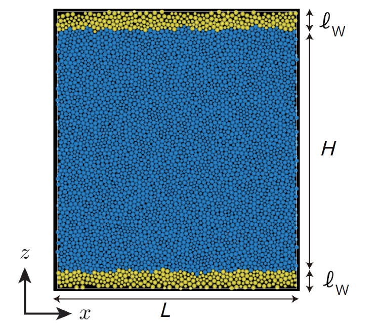
Figure 1: (Color online) Illustration of geometry. Large and small particles (in blue) are in a glassy state in the region $-H/2<z<H/2$. In top and bottom boundary layers with thickness $\ell_{\rm w}$, particles (in yellow) in a glassy configuration are bound by rigid springs to pinning centers ${\mbox{\boldmath$R$}}_{k}$ in the layers. The periodic boundary condition is imposed along the horizontal axes (axis for $d=2$) with period $L$. These unbound and bound particles interact via pairwise potentials. Their interfaces are irregular and rigid, so no slip occurs when the walls are slightly shifted along the $x$ axis.

As illustrated in Fig,1, we induce shear deformations by motions of boundary wallsShiba ; Maeda , which are in the regions $-\ell_{\rm w}<z+H/2<0$ at the bottom and $0<z-H/2<\ell_{\rm w}$ at the top with $\ell_{\rm w}\ll H$. To each layer, $M$ particles are bound by spring potentials $\psi(|{\mbox{\boldmath$r$}}_{k}-{\mbox{\boldmath$R$}}_{k}|)$, where ${\mbox{\boldmath$r$}}_{k}$ are the positions of these particles and ${\mbox{\boldmath$R$}}_{k}$ are the pinning centers fixed to the layers. We set $N<k\leq N+M$ at the top and $N+M<k\leq N+2M$ at the bottom. We assume the simple harmonic potential,

$$\psi(r)=\frac{1}{2}s_{0}r^{2}.$$ (2)

Pinning becomes stronger with increasing the coefficient $s_{0}$. The bound particles also belong to either of the first or second species in the bulk and their density is equal to the bulk density, so $M=N\ell_{\rm w}/H$.

Particle pairs $i\in a$ and $j\in b$ (including the bound ones) interact via short-ranged potentials $\phi_{ab}(r_{ij})$, where $r_{ij}=|{\mbox{\boldmath$r$}}_{i}-{\mbox{\boldmath$r$}}_{j}|$ and $a$ and $b$ denote the particle species ($1$ or $2$). As a result, the unbound particles do not penetrate into the boundary layers. For simplicity, we write $\phi_{ij}=\phi_{ab}(r_{ij})$ and $\psi_{k}=\psi(|{\mbox{\boldmath$r$}}_{k}-{\mbox{\boldmath$R$}}_{k}|)$. At fixed ${\mbox{\boldmath$R$}}_{k}$, the total potential energy is given by

$$U=\frac{1}{2}\sum_{i,j}\phi_{ij}+\sum_{k>N}\psi_{k},$$ (3)

where we sum over all the particles in the first term and the bound ones in the second term $(k>N$). We write the momentum density as ${\mbox{\boldmath$J$}}=\sum_{i}{\mbox{\boldmath$p$}}_{i}\delta({\mbox{\boldmath$r$}}-{\mbox{\boldmath$r$}}_{i})$ using the $\delta$ function. Since the force ${\mbox{\boldmath$f$}}_{i}=-\partial U/\partial{\mbox{\boldmath$r$}}_{i}$ on particle $i$ consists of the contributions from the particles and the walls, the time derivative ${\dot{\mbox{\boldmath$J$}}}=\partial{\mbox{\boldmath$J$}}/\partial t$ is written as

$${\dot{\mbox{\boldmath$J$}}}=-\nabla\cdot{\stackrel{{\scriptstyle\leftrightarrow}}{{\Pi}}}-\sum_{k>N}\delta({\mbox{\boldmath$r$}}-{\mbox{\boldmath$r$}}_{k})\nabla_{k}\psi_{k}.$$ (4)

Here, $\stackrel{{\scriptstyle\leftrightarrow}}{{\Pi}}=\{\Pi_{\alpha\beta}\}$ is the microscopic stress tensorIrving at position $r$ and the second term is the force density from the walls. Hereafter, the over-dot denotes taking the time-derivative, $\alpha$ and $\beta$ represent the Cartesian coordinates, and we set $\nabla_{i}^{\alpha}=\partial/\partial x_{i}^{\alpha}$ and $\nabla_{i}=(\nabla_{i}^{x},\nabla_{i}^{y},\nabla_{i}^{z})$.

We divide the stress tensor into kinetic and potential parts as $\Pi_{\alpha\beta}=\Pi_{\alpha\beta}^{\rm K}+\Pi_{\alpha\beta}^{\rm p}$ withIrving ; Onukibook

$$\Pi_{\alpha\beta}^{\rm K}({\mbox{\boldmath$r$}}) = \sum_{i}\frac{1}{m_{i}}p_{i\alpha}p_{i\beta}\delta({\mbox{\boldmath$r$}}-{\mbox{\boldmath$r$}}_{i}),$$ (5)

$$\Pi_{\alpha\beta}^{\rm p}({\mbox{\boldmath$r$}}) = -\sum_{i,j}\frac{1}{2r_{ij}}\phi_{ij}^{\prime}{x_{ij}^{\alpha}x_{ij}^{\beta}}\hat{\delta}({\mbox{\boldmath$r$}},{\mbox{\boldmath$r$}}_{i},{\mbox{\boldmath$r$}}_{j}),$$ (6)

where we sum over all the particles and set $\phi^{\prime}_{ij}=d\phi_{ij}/dr_{ij}$ and $x_{ij}^{\alpha}=x_{i}^{\alpha}-x_{j}^{\alpha}$ (the $\alpha$ component of ${\mbox{\boldmath$r$}}_{ij}={\mbox{\boldmath$r$}}_{i}-{\mbox{\boldmath$r$}}_{j}$). In Eq.(6), we introduce the Irving-Kirkwood $\delta$ function by

$${\hat{\delta}}({\mbox{\boldmath$r$}},{\mbox{\boldmath$r$}}_{i},{\mbox{\boldmath$r$}}_{j})=\int_{0}^{1}d\lambda\delta({\mbox{\boldmath$r$}}-\lambda{\mbox{\boldmath$r$}}_{i}-(1-\lambda){\mbox{\boldmath$r$}}_{j}),$$ (7)

which satisfies $\int d{\mbox{\boldmath$r$}}{\hat{\delta}}({\mbox{\boldmath$r$}},{\mbox{\boldmath$r$}}_{i},{\mbox{\boldmath$r$}}_{j})=1$ and is nonvanishing only when $r$ is on the line segment connecting ${\mbox{\boldmath$r$}}_{i}$ and ${\mbox{\boldmath$r$}}_{j}$. It follows the relation ${\mbox{\boldmath$r$}}_{ij}\cdot\nabla\hat{\delta}({\mbox{\boldmath$r$}},{\mbox{\boldmath$r$}}_{i},{\mbox{\boldmath$r$}}_{j})=\delta({\mbox{\boldmath$r$}}-{\mbox{\boldmath$r$}}_{j})-\delta({\mbox{\boldmath$r$}}-{\mbox{\boldmath$r$}}_{i})$, leading to $\sum_{\beta}\nabla_{\beta}\cdot{{\Pi}}^{\rm p}_{\alpha\beta}=\sum_{i,j}\delta({\mbox{\boldmath$r$}}-{\mbox{\boldmath$r$}}_{i})\nabla_{i}^{\alpha}\phi_{ij}$ in Eq.(4). If we integrate $z{\dot{J}}_{\alpha}$ in a region containing all the particles, Eq.(4) gives a useful relation,

$$\int d{\mbox{\boldmath$r$}}\Pi_{z\alpha}({\mbox{\boldmath$r$}})-\int d{\mbox{\boldmath$r$}}z{\dot{J}}_{\alpha}({\mbox{\boldmath$r$}})=\sum_{k>N}z_{k}\nabla_{k}^{\alpha}\psi_{k},$$ (8)

where the right hand side arises from the wall potentials.

We next move the top wall by $\gamma_{\rm ex}H/2$ and the bottom wall by $-\gamma_{\rm ex}H/2$ along the $x$ axis. Here $\gamma_{\rm ex}$ is a small mean shear strain, which can depend on time. Then, in $U$ in Eq.(3), the positions ${\mbox{\boldmath$R$}}_{k}$ are shifted by $\pm\gamma_{\rm ex}H/2$ along the $x$ axis and $\psi_{k}$ are changed by $\mp(\gamma_{\rm ex}H/2)(\partial\psi_{k}/\partial x_{k})$ to linear order in $\gamma_{\rm ex}$. Thus, $U$ is changed by $-\gamma_{\rm ex}{\cal A}$ with

$${\cal A}=\frac{H}{2}(F_{\rm bot}^{x}-F_{\rm top}^{x})=\frac{H}{2}\Big{(}\sum_{k\in{\rm top}}-\sum_{k\in{\rm bot}}\Big{)}\nabla_{k}^{x}\psi_{k}.$$ (9)

where $F_{\rm top}^{\alpha}=-\sum_{k\in{\rm top}}\nabla_{k}^{\alpha}\psi_{k}$ is the force on the particles from the top wall and $F_{\rm bot}^{\alpha}=-\sum_{k\in{\rm bot}}\nabla_{k}^{\alpha}\psi_{k}$ is that from the bottom wall. In Eq.(9), $\cal A$ consists of the contributions from the bound particles ($k>N$) and is amplified by the prefactor $H/2$. Hereafter, for any $a_{k}$, we write $(\sum_{k\in{\rm top}}-\sum_{k\in{\rm bot}})a_{k}=\sum_{k\in{\rm top}}a_{k}-\sum_{k\in{\rm bot}}a_{k}$. Previously, Shiba and one of the present authorsShiba applied a shear flow in the geometry in Fig.1 to binary particle systems in various states.

For $\alpha=x$, the right hand side of Eq.(8) is rewritten as ${\cal A}+\sum_{k>N}\delta z_{k}\nabla_{k}^{x}\psi_{k}$, where $\delta z_{k}=z_{k}\mp H/2$ at the top and the bottom layers, so it is nearly equal to $\cal A$ for $|\delta z_{k}|<\ell_{\rm w}\ll H$. Thus, $\cal A$ can also be expressed as a difference of two bulk integrals,

$${\cal A} = \int d{\mbox{\boldmath$r$}}\Pi_{zx}({\mbox{\boldmath$r$}})-\int d{\mbox{\boldmath$r$}}z{\dot{J}}_{x}({\mbox{\boldmath$r$}})$$ (10)

$$= \int d{\mbox{\boldmath$r$}}\Pi_{zx}^{\rm p}({\mbox{\boldmath$r$}})-\sum_{i}z_{i}f_{i}^{x}.$$

Here, the kinetic parts cancel from the relation $\int d{\mbox{\boldmath$r$}}z{\dot{J}}_{z}=d(\sum_{i}z_{i}p_{i}^{x})/dt=\sum_{i}[p_{i}^{z}p_{i}^{x}/m_{i}+z_{i}f_{i}^{x}]$. In the second line, $f_{i}^{x}$ is the $x$ component of the force ${\mbox{\boldmath$f$}}_{i}=-\partial U/\partial{\mbox{\boldmath$r$}}_{i}$ on particle $i$, so the sum $\sum_{i}z_{i}f_{i}^{x}$ is the off-diagonal virial. Since $U$ includes the wall potentials, the total force on the particles is given by

$$\sum_{i}{\mbox{\boldmath$f$}}_{i}={\mbox{\boldmath$F$}}_{\rm top}+{\mbox{\boldmath$F$}}_{\rm bot}.$$ (11)

Note that we can also move the top wall by $\gamma_{\rm ex}(H/2-a)$ and the bottom wall by $-\gamma_{\rm ex}(H/2+a)$, where $a$ is an arbitrary length. For example, the top wall is at rest for $a=H/2$. Then, ${\cal A}$ in Eq.(9) is changed to ${\cal A}^{\prime}=(H/2+a)F_{\rm bot}^{x}-(H/2-a)F_{\rm top}^{x}$ and $z_{i}$ in Eq.(10) is changed to $z_{i}-a$. Our expressions for $\mu$ will not depend on $a$ (see the sentences below Eqs.(44) and (50) and Eq.(51)).

II.2 Inherent state and quasi-equilibrium in glass

Glasses are nonergodic at low $T$, where the configuration changes are negligible during the observation in the limit of small applied strain. In the corresponding inherent state in the limit $T\to 0$, we write the particle positions as ${\mbox{\boldmath$r$}}_{i}={\mbox{\boldmath$r$}}_{i}^{\rm ih}=(x^{\rm ih}_{i},y^{\rm ih}_{i},z^{\rm ih}_{i})$, for which the mechanical equilibrium (${f}_{i}^{\alpha}=-\nabla_{i}^{\alpha}{U}={0}$) holds for all the particles. Thus, each inherent state is one of the local minima in the many-particle phase space. In addition, the inherent (residual) shear stress $\Pi_{\alpha\beta}^{\rm ih}({\mbox{\boldmath$r$}})=\lim_{T\to 0}\Pi_{\alpha\beta}({\mbox{\boldmath$r$}})$ is highly heterogeneous with long-range correlationsHarro ; Egami ; Lema ; Fuchs ; Seme . In our case, from Eqs.(9) and (10), the total shear stress is related to the force difference as

$$W^{\rm ih}=\int d{\mbox{\boldmath$r$}}\Pi_{zx}^{\rm ih}({\mbox{\boldmath$r$}})=\frac{1}{2}H(F_{\rm bot}^{x}-F_{\rm top}^{x})\quad(T\to 0),$$ (12)

while the total applied force ${\mbox{\boldmath$F$}}_{\rm bot}+{\mbox{\boldmath$F$}}_{\rm top}$ vanishes as $T\to 0$ from Eq.(11). Fuereder and IlgIlg found a counterpart of Eq.(12) in the periodic boundary condition. See more discussions on $\Pi_{zx}^{\rm ih}({\mbox{\boldmath$r$}})$ in Sec.IIH.

We next consider the particle displacements,

$${\mbox{\boldmath$u$}}_{i}=(u_{i}^{x},u_{i}^{y},u_{i}^{z})={\mbox{\boldmath$r$}}_{i}-{\mbox{\boldmath$r$}}_{i}^{{\rm ih}},$$ (13)

from the inherent positions. To leading order, the effective Hamiltoninan for ${\mbox{\boldmath$u$}}_{i}$ is of the bilinear form,

$${\cal H}_{\rm ih}=\sum_{i}\frac{1}{2m_{i}}|{\mbox{\boldmath$p$}}_{i}|^{2}+\delta U,$$ (14)

where ${\mbox{\boldmath$p$}}_{i}=m_{i}{\dot{\mbox{\boldmath$u$}}}_{i}$ and the potential part $\delta U$ is given by

$$\delta U=\frac{1}{4}\sum_{i,j,\alpha,\beta}{s_{ij}^{{\alpha\beta}}}{u}_{ij}^{\alpha}u_{ij}^{\beta}+\frac{1}{2}\sum_{k>N,\alpha}s_{0}|{{u}_{k}^{\alpha}}|^{2}.$$ (15)

The first term depends on $u_{ij}^{\alpha}=u_{i}^{\alpha}-u_{j}^{\alpha}$. We define

$$s_{ij}^{{\alpha\beta}}=\nabla_{i}^{\alpha}\nabla_{i}^{\beta}\phi_{ij}=(\frac{\phi_{ij}^{\prime\prime}}{r_{ij}^{2}}-\frac{\phi_{ij}^{\prime}}{r_{ij}^{3}})x_{ij}^{\alpha}x_{ij}^{\beta}+\frac{\phi_{ij}^{\prime}}{r_{ij}}\delta_{\alpha\beta},$$ (16)

where $\phi_{ij}^{\prime\prime}=d^{2}\phi_{ij}/dr_{ij}^{2}$ and the particle positions are at ${\mbox{\boldmath$r$}}_{i}={\mbox{\boldmath$r$}}_{i}^{\rm ih}$. For simplicity, $x_{i}^{\rm ih}$, $y_{i}^{\rm ih}$, and $z_{i}^{\rm ih}$ will be written as $x_{i}$, $y_{i}$, and $z_{i}$, when confusion will not occur.

The ${\cal H}_{\rm ih}$ describes the local vibrational motions in local potential minima and the collective acoustic modes on larger scales. We assume that the the observation time is much longer than the microscopic times but is much shorter than the structural relaxation time (see Sec.IIIA). Then, quasi-equilibrium should be attained at fixed ${\mbox{\boldmath$r$}}_{i}^{\rm ih}$, where $({\mbox{\boldmath$u$}}_{i},{\mbox{\boldmath$p$}}_{i}$) obey the canonical distribution,

$$P_{\rm ih}\propto\exp(-{\cal H}_{\rm ih}/k_{B}T).$$ (17)

Hereafter, the thermal average over this distribution will be written as $\langle{\cdots}\rangle_{\rm ih}=\int\Pi_{i=1}^{N+2M}d{\mbox{\boldmath$p$}}_{i}d{\mbox{\boldmath$u$}}_{i}(\cdots)P_{\rm ih}$ for a fixed inherent state (isoinherent ensemble). For simplicity, we assume the Gaussian form of $P_{\rm ih}$ to obtain $\langle{u_{i}^{\alpha}u_{j}^{\beta}}\rangle_{\rm ih}\propto k_{B}T$. However, there is no difficulty to include the anharmonic potential terms, which can be important with increasng $T$ (see a remark below Eq.(42))Sastry .

To linear order, the force on particle $i$ is written as

$$f_{i}^{\alpha}=-\frac{\partial}{\partial u_{i}^{\alpha}}{\delta U}=-\sum_{j,\beta}h_{ij}^{\alpha\beta}u_{j}^{\beta}.$$ (18)

From Eq.(15) the Hessian matrix $\{h_{ij}^{\alpha\beta}\}$ is symmetric as

$$h_{ij}^{\alpha\beta}=\sum_{k}s^{\alpha\beta}_{ik}\delta_{ij}-s_{ij}^{\alpha\beta}+s_{0}\delta_{\alpha\beta}\delta_{ij}\theta_{i-N},$$ (19)

where $\theta_{i-N}$ is 1 for $i>N$ and 0 for $i\leq N$. The last term is the contribution from the bound particles at the walls and is nonexistent in the periodic boundary condition.

The potential energy deviation in Eq.(15) assumes the symmetric bilinear form $\delta U=\sum_{i,j,\alpha,\beta}h_{ij}^{\alpha\beta}u_{i}^{\alpha}u_{j}^{\beta}/2$. Thus, the inverse matrix of $\{h_{ij}^{\alpha\beta}\}$ is related to the displacement variances as

$$(h^{-1})_{ij}^{\alpha\beta}=\langle{u_{i}^{\alpha}u_{j}^{\beta}}\rangle_{\rm ih}/k_{B}T,$$ (20)

From $f_{i}^{\alpha}=k_{B}T\partial(\ln P_{\rm ih})/\partial u_{i}^{\alpha}$, any variable $\cal B$ satisfies

$$-\langle{{\cal B}{f}_{i}^{\alpha}}\rangle_{\rm ih}=\sum_{k,\beta}h_{ik}^{\alpha\beta}\langle{u_{k}^{\beta}{\cal B}}\rangle_{\rm ih}=k_{B}T\langle{{\partial{\cal B}}/{\partial u_{i}^{\alpha}}}\rangle_{\rm ih}.$$ (21)

For ${\cal B}=u_{i}^{\alpha}$ we find $\langle{u_{i}^{\alpha}f_{j}^{\beta}}\rangle_{\rm ih}=-k_{B}T\delta_{ij}\delta_{\alpha\beta}.$ See a similar relation in Eq.(69) in equilibrium.

Many authorsSch ; Liu ; Yama ; Gelin ; Barr1 ; Barr2 ; Malo ; Elliott have calculated the vibrational modes in glasses in the periodic boundary condition. We can examine them with boundary walls by including the last term in Eq.(19) (see Fig.2).

II.3 $\Pi_{\alpha\beta}^{\rm p}$ and $\cal A$ around an inherent state

Around an inherent state, the potential part of the stress tensor $\Pi_{\alpha\beta}$ in Eq.(6) is expanded as

$$\Pi^{\rm p}_{\alpha\beta}({\mbox{\boldmath$r$}})=\Pi_{\alpha\beta}^{\rm ih}({\mbox{\boldmath$r$}})+\delta\Pi^{\rm p}_{\alpha\beta}({\mbox{\boldmath$r$}})+\cdots.$$ (22)

The first term is the inherent stress and the second term is the first-order deviation linear in ${\mbox{\boldmath$u$}}_{i}$ given by

$$\delta\Pi^{\rm p}_{\alpha\beta}({\mbox{\boldmath$r$}})=-\frac{1}{2}\sum_{i,j,\nu}w_{ij}^{{\alpha\beta}\nu}u_{ij}^{\nu}{\hat{\delta}}({\mbox{\boldmath$r$}},{\mbox{\boldmath$r$}}_{i},{\mbox{\boldmath$r$}}_{j})$$

$$+\sum_{i,j}\frac{{\phi_{ij}^{\prime}}{x_{ij}^{\alpha}}}{r_{ij}}({\mbox{\boldmath$u$}}_{i}\cdot\nabla)[(x_{\beta}-x_{j}^{\beta}){\hat{\delta}}({\mbox{\boldmath$r$}},{\mbox{\boldmath$r$}}_{i},{\mbox{\boldmath$r$}}_{j})].$$ (23)

In the first term the coefficients $w_{ij}^{{\alpha\beta}\nu}(=w_{ij}^{\beta\alpha\nu}=-w_{ji}^{{\alpha\beta}\nu}$) are defined in the inherent state by

$$w_{ij}^{{\alpha\beta}\nu}=\nabla_{i}^{\nu}[\phi_{ij}^{\prime}{x_{ij}^{\alpha}x_{ij}^{\beta}}/r_{ij}]=s_{ij}^{\alpha\nu}x_{ij}^{\beta}+\nabla_{i}^{\alpha}\phi_{ij}\delta_{\beta\nu}.$$ (24)

We derive the second term in Eq.(23) from the deviation of $\hat{\delta}$ in Eq.(7) using $x_{ij}^{\beta}{\mbox{\boldmath$u$}}_{i}\cdot\nabla_{i}{\hat{\delta}}=-{\mbox{\boldmath$u$}}_{i}\cdot\nabla[(x_{\beta}-x_{j}^{\beta}){\hat{\delta}}]$, which vanishes upon space integration. In this paper, we consider the space integral of $\delta\Pi_{zx}^{\rm p}({\mbox{\boldmath$r$}})$ written as

$$\delta W_{\rm p} = \int d{\mbox{\boldmath$r$}}\delta\Pi_{zx}^{\rm p}({\mbox{\boldmath$r$}})=-\frac{1}{2}\sum_{i,j,\alpha}w_{ij}^{zx\alpha}{u_{ij}^{\alpha}}$$ (25)

$$=-\sum_{i,\alpha}w_{i}^{\alpha}u_{i}^{\alpha},$$

where we can replace $u_{ij}^{\nu}=u_{i}^{\nu}-u_{j}^{\nu}$ in the first line by $2u_{i}^{\nu}$ to obtain the second line and we define the coefficients,

$$w_{i}^{\alpha}=\sum_{j}w_{ij}^{zx\alpha}=\sum_{j}[s_{ij}^{z\alpha}x_{ij}+\frac{\phi_{ij}^{\prime}}{r_{ij}}z_{ij}\delta_{x\alpha}].$$ (26)

From Eqs.(9), (10), and (25) the deviation of $\cal A$ is written to linear order in the following two forms,

$$\delta{\cal A}=\frac{1}{2}H(\delta F_{\rm bot}^{x}-\delta F_{\rm top}^{x})$$

$$\hskip 14.22636pt=\delta W_{\rm p}-\sum_{i}z_{i}f_{i}^{x}.$$ (27)

Here, $\delta F_{\rm top}^{\alpha}$ is the deviation of the force from the top wall and $\delta F_{\rm bot}^{\alpha}$ is that from the bottom wall, so

$$\delta F_{\rm top}^{\alpha}=-s_{0}\sum_{k\in{\rm top}}u_{k}^{\alpha},\quad\delta F_{\rm bot}^{\alpha}=-s_{0}\sum_{k\in{\rm bot}}u_{k}^{\alpha}.$$ (28)

We can also write $\delta{\cal A}=s_{0}\sum_{k>N}z_{k}u_{k}^{x}$ for $H\gg\ell_{\rm w}$.

II.4 Linear response in quasi-equilibrium

For a fixed inherent state, we use Kubo’s methodKubo in the linear response theory for the perturbed Hamiltonian,

$${\cal H}^{\prime}_{\rm ih}=\sum_{i}\frac{1}{2m_{i}}|{\mbox{\boldmath$p$}}_{i}|^{2}+\delta U-\gamma_{\rm ex}(t)\delta{\cal A}$$ (29)

around the quasi-equilibrium distribution $P_{\rm ih}$ in Eq.(17), where ${\delta U}$ and ${\delta{\cal A}}$ are given by Eqs.(15) and (27). The equations of motion are $\dot{\mbox{\boldmath$p$}}_{i}={\mbox{\boldmath$f$}}_{i}+\gamma_{\rm ex}\partial(\delta{\cal A})/\partial{\mbox{\boldmath$u$}}_{i}$ including the perturbation. As a result, the phase-space distribution slightly deviates from $P_{\rm ih}$. For any variable ${\cal B}$, we consider its time-dependent average over this perturbed distribution. Its deviation due to $\gamma_{\rm ex}$ is given by

$$\delta{\bar{\cal B}}(t)=\chi_{BA}(0)\gamma_{\rm ex}(t)-\int_{0}^{t}ds\chi_{BA}(t-s){\dot{\gamma}}_{\rm ex}(s),$$ (30)

where ${\dot{\gamma}}_{\rm ex}(t)=d\gamma_{\rm ex}(t)/dt$ and we assume ${\gamma}_{\rm ex}(t)=0$ for $t<0$. We define the response function,

$$\chi_{BA}(t)=\langle{{\cal B}(t)\delta{\cal A}(0)}\rangle_{\rm ih}/k_{B}T,$$ (31)

where the time-evolution is governed by the unperturbed Hamiltonian ${\cal H}_{\rm ih}$ in Eq.(14) (see Sec.IIG). The static susceptibility is given by the equal-time correlation in Eq.(30). Use of the second line of Eq.(27) gives

$$\chi_{BA}(0)=\frac{\langle{{\cal B}{\delta\cal A}}\rangle_{\rm ih}}{k_{B}T}=\langle{\sum_{i}z_{i}\frac{\partial{\cal B}}{\partial u_{i}^{x}}}\rangle_{\rm ih}+\frac{\langle{{\cal B}\delta W_{\rm p}}\rangle_{\rm ih}}{k_{B}T},$$ (32)

where the first term arises from the affine change in $\cal B$ and the second term is due to the correlation between $\cal B$ and the deviation $\delta W_{\rm p}$ in the total shear stress.

In particular, for a stepwise shear strain $\gamma_{\rm ex}(t)=\gamma_{0}\theta(t)$ (being 0 for $t<0$ and $\gamma_{0}$ for $t>+0$), we find

$$\delta{\bar{\cal B}}(t)/\gamma_{0}=\chi_{BA}(0)-\chi_{BA}(t)\quad(t>0).$$ (33)

For ${\cal B}=\delta W_{\rm p}$, we obtain the stress relaxation function $G_{\rm ih}(t)=-\delta{\bar{W}}_{\rm p}(t)/\gamma_{0}$ for $t>0$. From Eq.(33) we find

$$G_{\rm ih}(t)=\mu+\langle{\delta W_{\rm p}(t)\delta{\cal A}(0)}\rangle_{\rm ih}/k_{B}TV,$$ (34)

where $\mu$ is the average shear modulus in Eq.(38) below, so $G_{\rm ih}(0)=0$. Our $\chi_{BA}(t)$ and $G_{\rm ih}(t)$ exhibit oscillatory behavior and can be used only for $t$ before appreciable structural relaxation (see Fig.7). However, in the literature of rheologySaw ; Doi ; Wit1 , the stress relaxation function is the sum of $\mu$ and the stress time-correlation function in Eq.(61) (divided by $k_{B}T$).

II.5 Displacement and stress in steady shear strain

Let us make further calculations for a steady shear strain $\gamma_{\rm ex}$. For ${\cal B}=u_{i}^{\alpha}$, the first line of Eq.(27) gives the average dispacements. With the aid of Eq.(28) we find

$$\frac{{\bar{u}}_{i}^{\alpha}}{\gamma_{\rm ex}}=\frac{\langle{{u_{i}^{\alpha}}{\delta\cal A}}\rangle_{\rm ih}}{k_{B}T}=\frac{Hs_{0}}{2}\Big{(}\sum_{k\in{\rm top}}-\sum_{k\in{\rm bot}}\Big{)}(h^{-1})_{ik}^{\alpha x}.$$ (35)

Here, all $u_{i}^{\alpha}$ are coupled with the force difference $\delta F_{\rm bot}^{x}-\delta F_{\rm top}^{x}$. See Sec.IIF for more discussions on $\delta F_{\rm bot}^{x}$ and $\delta F_{\rm top}^{x}$. Furthermore, Eq.(32) gives another expression,

$$\frac{{\bar{u}}_{i}^{\alpha}}{\gamma_{\rm ex}}=z_{i}\delta_{\alpha x}-\sum_{k,\beta}(h^{-1})_{ik}^{\alpha\beta}w_{k}^{\beta},$$ (36)

which consists of the affine and nonaffine partsMalo .

For ${\cal B}=\delta\Pi_{zx}^{\rm p}({\mbox{\boldmath$r$}})$, we define the local shear modulus by

$${\hat{\mu}}({\mbox{\boldmath$r$}})=-\langle{\delta{{\bar{\Pi}}}_{zx}^{\rm p}({\mbox{\boldmath$r$}})}\rangle/\gamma_{\rm ex}=-\langle{{\delta{\Pi}_{zx}^{\rm p}({\mbox{\boldmath$r$}})}\delta{\cal A}}\rangle_{\rm ih}/k_{B}T.$$ (37)

This ${\hat{\mu}}({\mbox{\boldmath$r$}})$ has the particle discreteness in an inherent state, so we need to integrate it in small squares or cubes in the cell to detect elastic heterogeneityMiz1 ; PabloP . The space average of ${\hat{\mu}}({\mbox{\boldmath$r$}})$ in the whole cell is simpler as

$$\mu=\int d{\mbox{\boldmath$r$}}\frac{{\hat{\mu}}({\mbox{\boldmath$r$}})}{V}=-\frac{\langle{\delta W_{\rm p}\delta{\cal A}}\rangle_{\rm ih}}{Vk_{B}T}=\sum_{i,\alpha}\frac{w_{i}^{\alpha}{\bar{u}}_{i}^{\alpha}}{V\gamma_{\rm ex}},$$ (38)

Then, as $T\to 0$, Eqs.(35) and (38) yield

$${\mu}=\frac{s_{0}}{2V}H\sum_{i,\alpha}\Big{(}\sum_{k\in{\rm top}}-\sum_{k\in{\rm bot}}\Big{)}w_{i}^{\alpha}(h^{-1})_{ik}^{\alpha x}.$$ (39)

which arises from the correlations between the bound and unbound particles.

From Eq.(36) we also find the well-known expression,

$${\mu}=\langle{\mu_{\infty}}\rangle_{\rm ih}-{{\langle{\delta W_{\rm p}^{2}}\rangle_{\rm ih}}}/{Vk_{B}T}.$$ (40)

where $\mu_{\infty}=\sum_{i}w_{i}^{x}z_{i}/V$ is the affine contribution,

$$\mu_{\infty}=\frac{1}{2V}\sum_{i,j}\bigg{[}(\frac{\phi_{ij}^{\prime\prime}}{r_{ij}^{2}}-\frac{\phi_{ij}^{\prime}}{r_{ij}^{3}})x_{ij}^{2}{z_{ij}^{2}}+\frac{\phi_{ij}^{\prime}}{r_{ij}}{z_{ij}^{2}}\bigg{]}$$ (41)

This $\mu_{\infty}$ was first introduced for fluids (see Eq.(57))Zwanzig . As $T\to 0$, $\langle{\mu_{\infty}}\rangle_{\rm ih}$ is equal to $\mu_{\infty}$ at the inherent positions ${\mbox{\boldmath$r$}}_{i}={\mbox{\boldmath$r$}}_{i}^{\rm ih}$, while the nonaffine part is proportional to the stress variance and is negative. As $T\to 0$, we find

$$\langle{(\delta W_{\rm p})^{2}}\rangle_{\rm ih}/Vk_{B}T=\sum_{i,j,\alpha,\beta}(h^{-1})^{\alpha\beta}_{i,j}w_{i}^{\alpha}w_{j}^{\beta}/V.$$ (42)

We can use Eq.(40) even if we include the anharmonic potential terms in the average $\langle{\cdots}\rangle_{\rm ih}$ (see a comment below Eq.(17)). For large $V$, the bulk contributions dominate over the surface ones in Eqs.(40)-(42). See Appendix A for counterparts of Eqs.(40)-(42) in one dimension.

From Eqs.(27) and (30) the average of $\delta{\cal A}$ is given by

$${\delta{\bar{\cal A}}}/{\gamma_{\rm ex}}={\langle{(\delta{\cal A})^{2}}\rangle_{\rm ih}}/{k_{B}T}=s_{0}H^{2}M/2-\mu V,$$ (43)

where we use $\langle{\delta{\cal A}\sum_{i}z_{i}f_{i}^{x}}\rangle_{\rm ih}/k_{B}T=-s_{0}\sum_{i>N}z_{i}^{2}$. Since $\langle{\delta{\cal A}^{2}}\rangle_{\rm ih}>0$, we require $s_{0}>2\mu V/H^{2}M$, which is well satisfied in our simulation in Sec.IV. From Eqs.(27), (28), and (43) we can also express $\mu$ as

$$\mu=\frac{1}{V}\sum_{i>N,j>N}{z_{i}z_{j}}[s_{0}\delta_{ij}-s_{0}^{2}\langle{u_{i}^{x}u_{j}^{x}}\rangle_{\rm ih}/k_{B}T].$$ (44)

in terms of the variances of the bound particles. This relation is invariant with respect to the coordinate shift along the $z$ axis ($z_{i}\to z_{i}-a$ and $z_{j}\to z_{j}-a$) (which can be proved from Eqs.(47) and (48) below).

In Eq.(15) we replace $u_{k}^{x}$ by $u_{k}^{x}\mp H\gamma_{\rm ex}/2$ for $k>N$ to obtain the change in the potential energy deviation,

$$\delta U^{\prime}=\delta U-\gamma_{\rm ex}\delta{\cal A}+\gamma_{\rm ex}^{2}s_{0}H^{2}M/2,$$ (45)

up to of order $\gamma_{\rm ex}^{2}$, Minimization of $\delta U^{\prime}$ with respect to $u_{i}^{\alpha}$ gives $f_{i}^{\alpha}+\gamma_{\rm ex}\partial(\delta{\cal A})/\partial u_{i}^{\alpha}=0$. This leads to Eqs.(35) and (36) with the aid of the first and second lines of Eq.(27). Note that this derivation of Eq.(36) is equivalent to that of Maloney and LemaîtreMalo ; Malo1 . Let us then calculate the minimum value of $\delta U^{\prime}$ by seting $u_{i}^{\alpha}$ equal to ${\bar{u}}_{i}^{\alpha}$ in Eq.(35) and $\delta{\cal A}$ equal to $\delta{\bar{\cal A}}$ in Eq.(43). In terms of $\mu$ in Eq.(38), it is simply written as

$$\delta{\bar{U}}^{\prime}=\mu\gamma_{\rm ex}^{2}V/2,$$ (46)

which is not obvious for inhomogeneous glassy systems.

We note the following. (i) For crystals, the shear moduli are expressed in the same form as in Eq.(40), where the thermal average is taken over the displacement fluctuations in a given crystal stateHess ; Ray ; Lutsko ; Hoover . For glasses, the average is taken over one inherent statesMalo ; Malo1 ; Evans ; Yoshi ; Ilg ; Saw . (ii) To examine elastic inhomogeneity in glasses, some authorsMiz1 ; PabloP divided the cell into small regions and integrated the average of the first term in Eq.(23) in each region (where $\hat{\delta}$ can be integrated in a simple form).

II.6 Fluctuations of forces from walls

We have introduced the forces from the walls to the particles in Eq.(9). We here examine the equal-time correlations among their thermal fluctuations and $u_{i}^{\alpha}$. From Eqs.(11) and (21) and $\sum_{j}h_{ij}^{\alpha\beta}=-s_{0}\theta_{i-N}\delta_{\alpha\beta}$, the total force deviation $\delta F_{\rm tot}^{\alpha}\equiv\delta F_{\rm top}^{\alpha}+\delta F_{\rm bot}^{\alpha}$ satisfies

$$\langle{u_{i}^{\alpha}\delta F_{\rm tot}^{\beta}}\rangle_{\rm ih}=-k_{B}T\delta_{\alpha\beta},$$ (47)

$$\langle{\delta F_{\rm tot}^{\alpha}\delta F_{\rm tot}^{\beta}}\rangle_{\rm ih}=2k_{B}Ts_{0}M\delta_{\alpha\beta}.$$ (48)

From Eq.(11) the left hand side of Eq.(47) is written as $\langle{u_{i}^{\alpha}\sum_{j}{\dot{p}}_{j}^{\beta}}\rangle_{\rm ih}=-\langle{{\dot{u}}_{i}^{\alpha}\sum_{j}p_{j}^{\beta}}\rangle_{\rm ih}$; then, Eq.(47) is obvious. From Eqs.(25) and (26) $\delta W_{\rm p}$ and $\delta F_{\rm tot}^{\alpha}$ are orthogonal as

$$\langle{\delta W_{\rm p}\delta F_{\rm tot}^{\alpha}}\rangle_{\rm ih}=0.$$ (49)

On the other hand, the $x$-component of the force difference $\delta F_{\rm top}^{x}-\delta F_{\rm bot}^{x}$ is proportional to $\delta{\cal A}$ as in Eq.(27), so its relations follow from Eqs.(35) and (43). Using Eq.(48) also, we find the cross correlation,

$$\langle{\delta F_{\rm top}^{x}\delta F_{\rm bot}^{x}}\rangle_{\rm ih}/k_{B}T=\mu V/H^{2}=\mu L^{d-1}/H.$$ (50)

See Appendices A and B for counterparts of Eq.(50) in simpler situations. Here, we argue that Eq.(50) is general for elastic films. Let us move the bottom layer by $-H\gamma_{\rm ex}$ with the top layer kept at rest (see the last paragraph of Sec.IIA). Then, $\delta{\cal A}$ is changed to $\delta{\cal A}^{\prime}=H\delta F_{\rm bot}^{x}$ in Eq.(29) and the average force from the top wall to the particles is given by $\langle{\delta F_{\rm top}^{x}\delta{\cal A}^{\prime}}\rangle_{\rm ih}/k_{B}T=\mu V/H$ in equilibrium, which coincides with Eq.(50). See Eq.(82) and Fig.8 for the time-correlation of the wall forces. In accord with this argument, Eqs.(38) and (49) give

$$\mu=-{\langle{\delta W_{\rm p}\delta{F}_{\rm bot}^{x})}\rangle_{\rm ih}}H/{Vk_{B}T},$$ (51)

where $\delta{F}_{\rm bot}^{x}$ can be replaced by $-\delta{F}_{\rm top}^{x}$.

II.7 Linear dynamics around a fixed inherent state

Around a fixed inherent state, the dynamic equations follow from ${\cal H}_{\rm ih}$ in Eq.(14). They are rewritten as

$$\frac{d^{2}}{dt^{2}}{\hat{u}}_{i}^{\alpha}(t)=-\sum_{j,\beta}{\hat{h}}_{ij}^{\alpha\beta}{\hat{u}}_{j}^{\beta}(t).$$ (52)

For $m_{1}\neq m_{2}$, we use the following scale changesElliott ; Yama ,

$${\hat{u}}_{i}^{\alpha}(t)=\sqrt{m_{i}}{u}_{i}^{\alpha}(t),\quad{\hat{h}}_{ij}^{\alpha\beta}={h}_{ij}^{\alpha\beta}/\sqrt{m_{i}m_{j}},$$ (53)

where ${\hat{h}}_{ij}^{\alpha\beta}$ is the modified Hessian matrix. Its inverse is given by ${({\hat{h}}^{-1})}_{ij}^{\alpha\beta}=\sqrt{m_{i}m_{j}}{(h^{-1})}_{ij}^{\alpha\beta}$. We introduce the $d(N+2M)$ dimensional eigenvectors $e^{\lambda}_{i\alpha}$ satisfying

$$\sum_{j,\beta}{\hat{h}}_{ij}^{{\alpha\beta}}e^{\lambda}_{j\beta}=\omega_{\lambda}^{2}e^{\lambda}_{i\alpha},$$ (54)

where $0<\omega_{1}\leq\omega_{2}\leq\cdots$. The $e_{i\alpha}^{\lambda}$ are normalized as $\sum_{\lambda}e^{\lambda}_{i\alpha}e^{\lambda}_{j\beta}=\delta_{\alpha\beta}\delta_{ij}$ and $\sum_{i,\alpha}e^{\lambda}_{i\alpha}e^{\sigma}_{i\alpha}=\delta_{\lambda\sigma}$. Projection of ${\hat{u}}_{i}^{\alpha}$ on the eigenmodes yields the variables $s_{\lambda}$ as

$$s_{\lambda}=\sum_{i,\alpha}e^{\lambda}_{i\alpha}{\hat{u}}_{i}^{\alpha},\quad{\hat{u}}_{i}^{\alpha}=\sum_{\lambda}e_{i\alpha}^{\lambda}s_{\lambda}.$$ (55)

The potential energy deviation in Eq.(15) is written as

$$\delta U=\frac{1}{2}\sum_{i,\alpha,j,\beta}{\hat{h}}_{ij}^{{\alpha\beta}}{\hat{u}}_{i}^{\alpha}{\hat{u}}_{j}^{\beta}=\frac{1}{2}\sum_{\lambda}\omega_{\lambda}^{2}s_{\lambda}^{2},$$ (56)

from which we find $\langle{s_{\lambda}s_{\sigma}}\rangle_{\rm ih}=k_{B}T\delta_{\lambda\sigma}/\omega_{\lambda}^{2}$.

Now, from Eqs.(52)-(55), we obtain the dynamic equations $d^{2}s_{\lambda}(t)/dt^{2}=-\omega_{\lambda}^{2}s_{\lambda}(t)$. These are solved to give $s_{\lambda}(t)=s_{\lambda}(0)\cos(\omega_{\lambda}t)+{\dot{s}}_{\lambda}(0)\sin(\omega_{\lambda}t)/\omega_{\lambda}.$ with ${\dot{s}}_{\lambda}(0)=\sum_{i,\alpha}e^{\lambda}_{i\alpha}\sqrt{m_{i}}{\dot{u}}_{i}^{\alpha}(0)$ being linear in the velocities at $t=0$. Thus, averaging over $P_{\rm ih}$ yields

$$\langle{s_{\lambda}(t)s_{\sigma}(0)}\rangle_{\rm ih}/k_{B}T=\delta_{\lambda\sigma}\cos(\omega_{\lambda}t)/\omega_{\lambda}^{2}.$$ (57)

For any variable $\delta{\cal B}(t)=\sum_{i,\alpha}b_{i}^{\alpha}u_{i}^{\alpha}(t)$ linear in $u_{i}^{\alpha}(t)$, we can express it as $\delta{\cal B}(t)=\sum_{\lambda}Z_{B}^{\lambda}s_{\lambda}(t)$, where

$$Z_{B}^{\lambda}=\sum_{i,\alpha}{b_{i}^{\alpha}}e_{i\alpha}^{\lambda}/{\sqrt{m_{i}}}.$$ (58)

Furthermore, if $\delta{\cal A}(t)=\sum_{\lambda}Z_{A}^{\lambda}s_{\lambda}(t)$, Eq.(57) gives

$$\chi_{BA}(t)=\frac{\langle{\delta{\cal B}(t)\delta{\cal A}(0)}\rangle_{\rm ih}}{k_{B}T}=\sum_{\lambda}Z_{B}^{\lambda}Z_{A}^{\lambda}\frac{\cos(\omega_{\lambda}t)}{\omega_{\lambda}^{2}}.$$ (59)

At $t=0$, Eq.(59) is the equal-time correlation from $\sum_{\lambda}e^{\lambda}_{i\alpha}\omega_{\lambda}^{-2}e^{\lambda}_{j\beta}={({\hat{h}}^{-1})}_{ij}^{\alpha\beta}$. The expressions (57) and (59) exhibit oscillation even at long times without dissipationGelin ; Elliott . In particular, if $\delta{\cal B}=u_{i}^{\alpha}$ and $\delta{\cal A}$ is given by Eq.(27), Eqs.(35), (55), and (59) lead to another expression for the average induced displacements,

$${\bar{u}}_{i}^{\alpha}/\gamma_{\rm ex}=\sum_{\lambda}e_{i\alpha}^{\lambda}Z_{A}^{\lambda}/(\sqrt{m_{i}}\omega_{\lambda}^{2}).$$ (60)

II.8 Stress time-correlation in simulation

The stress time-correlation function has been calculated via molecular dynamics simulationOnukibook ; Harro ; Zwan ; Hansen ; Green . Using the integral of the shear stress $W(t)=\int d{\mbox{\boldmath$r$}}\Pi_{zx}({\mbox{\boldmath$r$}},t)$ at time $t$ for large systems, we express it as

$$C(t)=\langle{W(t+t_{0})W(t_{0})}\rangle_{\rm sim}/V.$$ (61)

As in usual simulations, $\langle{\cdots}\rangle_{\rm sim}$ includes the average over a long time interval of the initial time $t_{0}\in[0,t_{\rm sim}]$. It can also be over many simulation runs or over many inherent states in glasses. For a suitable ensemble, the integral of the inherent stress $W^{\rm ih}=\int d{\mbox{\boldmath$r$}}\Pi^{\rm ih}$ can obey a distribution with $\langle{W^{\rm ih}}\rangle_{\rm sim}=0$ without applied strainHarro ; Ilg . Here, if $t$ and $t_{\rm sim}$ are sufficiently long at not very small $T$, $C(t)$ slowly decays to zero due to the configuration changes (see Sec,IIIA).

It is well-known that $C(t)$ decays from its initial value $C(0)$ to a well-defined plateau value $C_{\rm pl}$ after a microscopic time at low $T$. In our simulation in Sec.IV, this will be the case after averaging over $t_{0}$ even in a single run. Here, $C(0)$ and $C_{\rm pl}$ do not depend on the system size for large $V$. The $C_{\rm pl}$ is nearly independent of $T$ and is related to the inherent stress asIlg ; Harro ; Yoshi ; Evans ; Wil

$$C_{\rm pl}=\langle{(W^{\rm ih})^{2}}\rangle_{\rm sim}/V\quad(T\to 0),$$ (62)

From Eq.(12) we also find

$$\langle{(F_{\rm bot}^{x}-F_{\rm top}^{x})^{2}}\rangle_{\rm sim}=4C_{\rm pl}V/H^{2}\quad(T\to 0).$$ (63)

On the other hand, the kinetic stress and the potential stress deviation $\delta W_{\rm p}(t)$ decay rapidly in Eq.(61). Thus,

$$C(0)-C_{\rm pl}=n(k_{B}T)^{2}+\langle\langle{{\delta W_{\rm p}}^{2}}\rangle_{\rm ih}{\rangle}_{\rm sim}/V$$ (64)

where $n(k_{B}T)^{2}$ is the kinetic contribution with $n=N/V$ and $\langle{{\delta W_{\rm p}}^{2}}\rangle_{\rm ih}$ is given in Eq.(42) for each inherent state.

From Eqs.(40) and (64) the average of $\mu$ is written as

$$\langle{\mu}\rangle_{\rm sim}=(\langle{\mu_{\infty}}\rangle_{\rm sim}+nk_{B}T)-(C(0)-C_{\rm pl})/k_{B}T,$$ (65)

which holds at finite $T$. Since Eq.(11) indicates $F_{\rm bot}^{x}=-F_{\rm top}^{x}$ at $T=0$, Eqs.(62)-(65) yield the wall-force correlation including the inherent contribution,

$$\langle{F_{\rm bot}^{x}F_{\rm top}^{x}}\rangle_{\rm sim}H^{2}/V=k_{B}T\langle{\mu}\rangle_{\rm sim}-C_{\rm pl}$$

$$=k_{B}T(\langle{\mu_{\infty}}\rangle_{\rm sim}+nk_{B}T)-C(0).$$ (66)

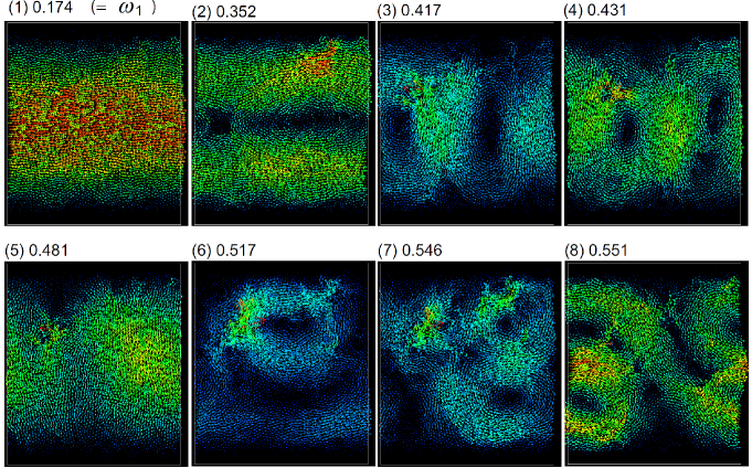
Figure 2: First eight normal modes $e_{i\alpha}^{\lambda}$ ($1\leq\lambda\leq 8$) in two dimensions with nearly rigid boundary walls at $z=\pm H/2$ and the periodic boundary condition along the $x$ axis, which are obtained from Eq.(54) with the normalization $\sum_{i,\alpha}(e_{i\alpha}^{\lambda})^{2}=1$. Number on each panel gives $\omega_{\lambda}$. Colors of the particles represent the displacement magnitude $|{\mbox{\boldmath$u$}}_{i}|$. The first and second modes correspond to the transverse sounds. The fifth mode is the first longitudinal sound. In the third, forth, and eighth modes, transverse and longitudinal displacements are mixed due to the walls. In the third, sixth and seventh modes, quasi-localized regions of large displacements can be seen in the upper left region.

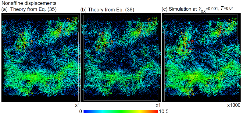
Figure 3: (Color online) Nonaffine displacements $({\bar{u}}_{i}^{x}/\gamma_{\rm ex}-z_{i},{\bar{u}}_{i}^{z}/\gamma_{\rm ex})$ divided by mean strain $\gamma_{\rm ex}$ in the $x$-$z$ plane $(d=2)$ at low $T$, where those of 4000 unbound particles can be seen but those of 500 bound particles are invisible. Colors represent magnitudes of these vectors. They are calculated from Eq.(35) in (a), from Eq.(36) in (b), and from simulation of applying a strain of $\gamma_{\rm ex}=10^{-3}$ at $T=0.01$ in (c). In (a) and (b), use is made of the inverse Hessian matrix $(h^{-1})_{ij}^{\alpha\beta}$. In (c), the particle displacements are completely reversible and the depicted positions are those averaged over a time interval of $5000$, where thermal vibrational motions are removed. Results in (a), (b), and (c) are very close to support our theory.

III Vanishing of shear modulus

III.1 Supercooled liquids

In supercooled liquids, the configuration changes occur appreciably on timescales longer than the bond breakage time $\tau_{b}$Kawasaki ; Yama1 ; Shiba . In each plastic event, some bonds are broken and some particles jump over distances longer than their diameters. As a result, the diffusion constants of the two componentsKawasaki become proportional to $\tau_{b}^{-1}$ with the coefficients independent of $T$. Therefore, the quasi-equilibrium distribution $P_{\rm ih}$ in Eq.(17) can be used on timescales shorter than $\tau_{b}$, where the mean-square displacements are smaller than the square of the particle diameters. At higher $T$, the second term in Eq.(65) increases such that $\langle{\mu}\rangle_{\rm sim}\to 0$ at a transition temperatureWil ; Evans ; Yoshi ; Saw ; Ilg ; Teren .

For shear rate ${\dot{\gamma}}_{\rm ex}$, we have a Newtonian regime for ${\dot{\gamma}}_{\rm ex}\tau_{b}<1$ and a shear-thinning regime for ${\dot{\gamma}}_{\rm ex}\tau_{b}>1$Kawasaki ; Yama1 ; Shiba , where the Newtonian viscosity is of order $\mu\tau_{b}$ and the nonlinear one is of order $\mu/{\dot{\gamma}}_{\rm ex}$. Note that the Green-Kubo formula for the former depends on the ensemble for deep supercoolingHarro ; Yip , where the average $\langle{\cdots}\rangle_{\rm sim}$ in Eq.(61) has to be still in some limited phase-space region.

III.2 Liquids

In liquids at higher $T$, thermal equilibration is rapidly achieved within experimental times. We can use the linear response theory around the equilibrium distribution $P_{\rm eq}\propto\exp(-{\cal H}/k_{B}T)$ with ${\cal H}=\sum_{i}|{\mbox{\boldmath$p$}}_{i}|^{2}/2m_{i}+U$. Here, the equilibrium average over $P_{\rm eq}$ is written as $\langle{\cdots}\rangle_{\rm eq}$.

If the boundaries are slightly moved, the perturbed Hamiltonian is ${\cal H}^{\prime}={\cal H}-\gamma_{\rm ex}(t){\cal A}$, where $\cal A$ is given in Eq.(9) with $\langle{{\cal A}}\rangle_{\rm eq}=0$. For any variable ${\cal B}$, its average response is thus expressed in the form of Eq.(30) with

$$\chi_{BA}(t)=\langle{{\cal B}(t){\cal A}(0)}\rangle_{\rm eq}/k_{B}T.$$ (67)

If ${\cal B}(t)=J_{x}({\mbox{\boldmath$r$}},t)=\sum_{i}p_{i}^{x}(t)\delta({\mbox{\boldmath$r$}}-{\mbox{\boldmath$r$}}_{i}(t))$ in Eq.(67), the response depends on $z$ and $t$. The resultant boundary flow profile will be investigated in future.

In liquids, the static shear modulus $\mu$ vanishes from $\langle{W{\cal A}}\rangle_{\rm eq}=0$, where $W=\int d{\mbox{\boldmath$r$}}\Pi_{\rm xy}$ is the total shear stress. Using $\mu_{\infty}$ in Eq.(41) we rewrite it as

$$\langle{\mu_{\infty}}\rangle_{\rm eq}+nk_{B}T=\langle{W^{2}}\rangle_{\rm eq}/Vk_{B}T,$$ (68)

where the left hand side is called the high-frequency shear modulusZwanzig . We can prove Eq.(68) using the relationZwanzig ,

$$\langle{{\cal B}f_{i}^{\alpha}}\rangle_{\rm eq}=-k_{B}T\langle{\partial{\cal B}/\partial x_{i}^{\alpha}}\rangle_{\rm eq}.$$ (69)

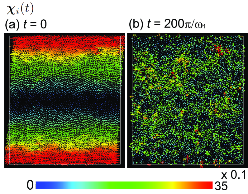
Figure 4: (Color online) Response functions $(\chi_{i}^{x}(t),\chi_{i}^{z}(t))$ in Eq.(76) obtained from Eq.(35), where (a) $t=0$ and (b) $t=200\pi/\omega_{1}$. Colors represent magnitudes of these vectors. Those in (a) are equal to normalized displacements $({\bar{u}}_{i}^{x}/\gamma_{\rm ex},{\bar{u}}_{i}^{z}/\gamma_{\rm ex})$, where the affine parts are dominant near the walls. In (b), small-amplitude vibrational modes can be seen, but the intial affine parts have disappeared.

For a small oscillatory shear rate ${\dot{\gamma}}_{\rm ex}={\dot{\gamma}}_{0}\cos(\omega t)$, the average shear stress is the real part of $-{\dot{\gamma}}_{0}\eta^{*}(\omega)e^{{\rm i}\omega t}$. From Eq.(10) we find the complex shear viscosity,

$$\eta^{*}(\omega)=\frac{1}{Vk_{B}T}\int_{0}^{\infty}dte^{-{\rm i}\omega t}\Big{[}\langle{W(t)W(0)}\rangle_{\rm eq}$$

$$\hskip 28.45274pt+{{\rm i}\omega}\langle{W(t){\cal G}_{x}(0)}\rangle_{\rm eq}\Big{]},$$ (70)

where ${\cal G}_{x}(t)=\int d{\mbox{\boldmath$r$}}zJ_{x}({\mbox{\boldmath$r$}},t)=\sum_{j}z_{j}(t){p}_{j}^{x}(t)$. At $\omega=0$, the Green-Kubo formula surely holds for the viscosity $\eta=\eta^{*}(0)$ in the bulk. We can also use the argument below Eq.(50) to fluids. For liquids, Eq.(30) gives

$$\eta=\frac{1}{Vk_{B}T}H^{2}\int_{0}^{\infty}dt\langle{F_{\rm top}^{x}(t)F_{\rm bot}^{x}(0)}\rangle_{\rm eq},$$ (71)

which should be compared with Eq.(50) for elastic films.

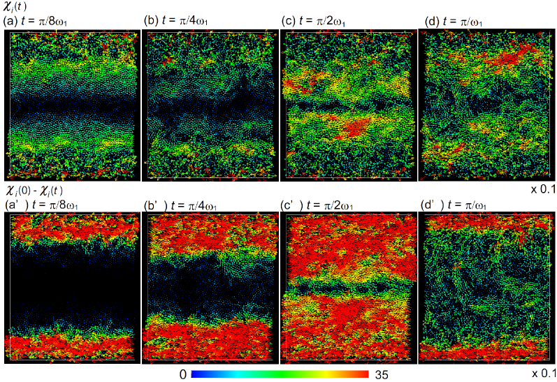
Figure 5: (Color online) Time-dependent response functions ${\bm{\chi}}_{i}(t)=(\chi_{i}^{x}(t),\chi_{i}^{z}(t))$ in Eq.(76) (top) and differences ${\bm{\chi}}_{i}(0)-{\bm{\chi}}_{i}(t)$ in Eq.(77) (bottom) in the $x$-$z$ plane $(d=2)$, where $\omega_{1}t$ is $\pi/8$, $\pi/4$, $\pi/2$, and $\pi$ (in the first half period) with $\omega_{1}=0.174(\cong\pi c_{\perp}/H)$. Top: Affine correlation at $t=0$ disappears as transverse sounds propagate inward with speed $c_{\perp}=3.9$ from the walls. Bottom: These are normalized disturbances after stepwise wall motions at $t=0$, which propagate from the walls and meet at $t=\pi/2\omega_{1}$. Colors represent the magnitudes of these vectors. These are calculated from the linear-response relations in Sec.IIG.

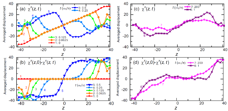
Figure 6: (Color online) Laterally averaged response function (x component) ${\bar{\chi}}^{x}(z,t)$ (top) and ${\bar{\chi}}^{x}(z,0)-{\bar{\chi}}^{x}(z,t)$ (bottom) as functions of $z$. These are defined in Eq.(78) in the range $|z|<H/2+\ell_{\rm w}$. Normalized time $\omega_{1}t/\pi$ is $0,1/16,1/8,1/4,$ and $1/2$ in (a) and (b) and is 1 and 200 in (c) and (d). In (a), the initial affine correlations disappear with propagation of transverse sounds from the walls. Relaxation at the walls takes place on a timescale of $\tau_{\rm w}\sim 2$. In (b), the boundary displacements propagate inward with $c_{\perp}$ as a shock wave with front thickness $c_{\perp}\tau_{\rm w}$. In (c) and (d), the correlations decay very slowly at long times.

IV Numerical results in two dimensions

IV.1 Simulation method

We now present numerical results in two dimensions ($d=2$) in the $x$-$z$ plane. We have briefly described our model at the beginning of Sec.II. Our system is composed of two particle species with numbers $N_{1}=N_{2}=N/2=2000$ in the cell. The pairwise potentials are given by

$$\phi_{ab}(r)=\epsilon{[(\sigma_{a}+\sigma_{b})/2]}^{12}[{r}^{-12}-r_{c}^{-12}]\quad(r<r_{\rm c}),$$ (72)

where $a$ and $b$ represent the particle species and we introduce $\epsilon$, $\sigma_{1}$, and $\sigma_{2}=1.4\sigma_{1}$. The potentials $\phi_{ab}(r)$ vanish for $r\geq r_{\rm c}=2.25(\sigma_{a}+\sigma_{b})$. The mass ratio is $m_{2}/m_{1}=1.96$. The cell lengths are $H=L=70.2\sigma_{1}$. The average particle density is $n=N/LH=0.81\sigma_{1}^{-2}$ and the average mass density is $\rho=1.2m_{1}\sigma_{1}^{-2}$. Hereafter, we will measure space, time, and temperature in units of $\sigma_{1}$, $t_{0}=\sigma_{1}(m_{1}/\epsilon)^{1/2}$, and $\epsilon/k_{B}$, respectively.

As in Fig.1, we attach two boundary layers with thickness $\ell_{\rm w}=H/16$. Each layer contains $M=250$ particles bound to pinning points ${\mbox{\boldmath$R$}}_{j}$ by the potential (2). The total particle number is $N+2M=4500$. The ${\mbox{\boldmath$R$}}_{j}$ were particle positions in a liquid stateShiba . The spring constant is chosen to be large at $s_{0}=200$. Then, the displacements of the bound particles from their inherent positions $u_{k}^{\alpha}$ ($k>N$) undergo thermal motions with amplitudes of order $(T/s_{0})^{1/2}=0.07T^{1/2}\ll 1$. Under applied strain, the motions of the bound particles are very small $(\propto s_{0}^{-1}$), which become even smaller with increasing the distance from the cell region. Our walls are nearly rigid and their surfaces are rough as in Fig.1, so slip motions do not occur for small wall motions.

We followed the following steps. (i) We started with a liquid at high $T$, lowered $T$ to 0.01 without crystallization, and waited for a time of $10^{3}$ to realize a glassy state, where we attached Nosé-Hoover thermostats in the cell and in the boundary layersShiba . (ii) We carried out some simulation runs at $T=0.01$ removing the thermostats. Results from these runs will be presented in Fig.3(c) and Fig.7(a). (iii) To seek an inherent state, we further cooled our system down to $T=10^{-5}$ keeping the thermostats without applied strain. Then, the particle positions became frozen. We use the resultant inherent state in Figs.2-9 without taking the ensemble average.

IV.2 Inherent state and eigenmodes

First, we examine the validity of Eqs.(62) and (63) in the limit $T\to 0$. Indeed, we obtain $(W^{\rm ih})^{2}/V=31.1$ and $(H^{2}/4V){(F_{\rm bot}^{x}-F_{\rm top}^{x})^{2}}=32.2$, while we find the plateau value $C_{\rm pl}=27.7$ from a simulation run at $T=0.01$. These three values are fairly close even for a single inherent state. For the inherent particle positions, we calculated the coefficients $w_{i}^{\alpha}$ in Eq.(26), the Hessian matrix $h_{ij}^{\alpha\beta}$ in Eq.(19), and its inverse $(h^{-1})_{ij}^{\alpha\beta}$ satisfying Eq.(20). The product of these two matrices is very close to the unit matrix $\delta_{\alpha\beta}\delta_{ij}$ with differences of order $10^{-16}$ for all the elements. The shear modulus $\mu$ is then given by $18.1$ from Eq.(39), $15.4$ from Eq.(40), $17.4$ from Eqs.(44) and (50), while it is $16.0$ from the stress-strain relation obtained from a simulation in Fig.3(c).

In Fig.2, we display the first eight eigenvectors $e_{i\alpha}^{\lambda}$, where the displacements of the bound particles are very small and are invisible here. The lowest eigenfrequency is $\omega_{1}=0.174$. This corresponds to the first transverse sound mode $e_{i\alpha}^{1}$, which is roughly proportional to $\delta_{\alpha x}\sqrt{m_{i}}\cos(\pi z_{i}/H)$ $(i\leq N)$. If we set $\omega_{1}=\pi c_{\perp}/H$, we obtain the transverse sound speed $c_{\perp}=3.9$. The same speed follows from $c_{\perp}=(\mu/\rho)^{1/2}$ for $\mu=16$ and $\rho=1.2$. The first longitudinal mode appears at $\lambda=5$ with $\omega_{5}=0.481$. We also obtain strongly localized modes for $\lambda=6$ and $7$, where clusters of large-amplitude oscillation are weakly connected to the bulkSch .

We project the variables $\delta W_{\rm p}$ in Eq.(25) and $\delta{\cal A}$ in Eq.(27) on the eigenmodes as $\delta W_{\rm p}=\sum_{\lambda}Z_{W}^{\lambda}s_{\lambda}$ and $\delta{\cal A}=\sum_{\lambda}Z_{A}^{\lambda}s_{\lambda}$ (see Sec.IIG). Here, Eq.(58) gives

$$Z_{W}^{\lambda}=-\sum_{i,\alpha}\frac{w_{i}^{\alpha}e_{i\alpha}^{\lambda}}{\sqrt{m_{i}}},~{}Z_{A}^{\lambda}=(\sum_{k\in{\rm bot}}-\sum_{k\in{\rm top}})\frac{Hs_{0}e_{kx}^{\lambda}}{2\sqrt{m_{k}}}.$$ (73)

From Eq.(38), $\mu$ is expressed as

$$\mu=-\frac{\langle{\delta W_{\rm p}\delta{\cal A}}\rangle_{\rm ih}}{k_{B}TV}=-\sum_{\lambda}\frac{Z_{W}^{\lambda}Z_{A}^{\lambda}}{\omega_{\lambda}^{2}V},$$ (74)

which is calculated to be 17.7. In Table 1, we give $\omega_{\lambda}$, $Z_{W}^{\lambda}$, and $Z_{A}^{\lambda}$ ($\lambda\leq 8$) for the inherent state under consideration, where $Z_{A}^{\lambda}$ have large amplitudes as compared to $Z_{W}^{\lambda}$. In fact, we find $\langle{(\delta{\cal A})^{2}}\rangle_{\rm ih}/k_{B}T=\sum_{\lambda}(Z_{A}^{\lambda})^{2}/\omega_{\lambda}^{2}=2.5\times 10^{4}V$ from Eq.(43), while we calculate $\langle{(\delta{W}_{\rm p})^{2}}\rangle_{\rm ih}/k_{B}T=\sum_{\lambda}(Z_{W}^{\lambda})^{2}/\omega_{\lambda}^{2}=21.2V$. Notice that Eq.(26) also gives $Z_{W}^{\lambda}=-\sum_{i,j,\alpha}w_{ij}^{zx\alpha}E_{ij\alpha}^{\lambda}/2$, where $E_{ij\alpha}^{\Lambda}\equiv e_{i\alpha}^{\lambda}/{\sqrt{m_{i}}}-e_{j\alpha}^{\lambda}/{\sqrt{m_{j}}}$ are small for most adjacent $i$ and $j$. See Eq.(B8) for the eigenmode projection of $\delta{\cal A}$ in the continuum elasticity.

Table 1: Vibrational eigenmodes and projection coefficients.

${\lambda}$		1	2	3	4	5	6	7	8
$\omega_{\lambda}$		0.174	0.352	0.417	0.431	0.481	0.517	0.546	0.551
$Z_{W}^{\lambda}$		1.375	11.76	-0.226	-1.730	-7.920	-9.957	11.71	-13.64
$Z_{A}^{\lambda}$		37.83	-66.11	24.41	-13.08	231.3	-153.7	118.7	26.22

IV.3 Nonaffine displacements at static strain

In Fig.3, we display the normalized nonaffine displacements $({\bar{u}}_{i}^{x}/\gamma_{\rm ex}-z_{i},{\bar{u}}_{i}^{z}/\gamma_{\rm ex})$ for all the particles. They are highly heterogeneous on large scales for the unbound particles, as has been reported in the literaturePabloP ; Malo ; Malo2 ; Barr1 ; Barr2 ; Miz1 ; Liu ; Wit ; Wit1 . Those of the bound particles are small and invisible. To confirm the validity of our theory, we calculated these results (a) from the wall-particle correlations in Eq.(35), (b) from the particle-particle correlations in Eq.(36), and (c) from a single run of molecular dynamics simulation of applying a strain of $\gamma_{\rm ex}=10^{-3}$ at $T=0.01$. In (a) and (b), we use the inverse Hessian matrix and the results are the averages over $P_{\rm ih}$ in Eq.(17). In (c), use is made of the common inherent state, the time average is over a time interval of $t_{\rm sim}=5000$, and there is no irreversible motion. We can see good agreement of the results in (a), (b), and (c) from the three methods, which supports our theory. In particular, those in (a) and (c) are very close.

In Fig.4(a), we present the full normalized displacements $({\bar{u}}_{i}^{x}/\gamma_{\rm ex},{\bar{u}}_{i}^{z}/\gamma_{\rm ex})$ using Eq.(35), whose affine parts are conspicuous near the walls. Here, Eq.(60) gives

$$Z_{A}^{\lambda}=\omega_{\lambda}^{2}\sum_{i,\alpha}(e_{i\alpha}^{\lambda}/{\sqrt{m_{i}}})({{\bar{u}}_{i}^{\alpha}}/{\gamma_{\rm ex}}),$$ (75)

which is equivalent to the second relation in Eq.(73). If we set ${{\bar{u}}_{i}^{\alpha}}/{\gamma_{\rm ex}}=z_{i}\delta_{\alpha x}$ in Eq.(75), we obtain the affine part of $Z_{A}^{\lambda}$. For $\lambda=1$, it is $-0.54$, so $Z_{A}^{1}$ mostly consisits of the nonaffine part since $Z_{A}^{1}\cong 38$ (see Eq.(B8)).

IV.4 Space-dependent dynamics

Next, we examine space-time-dependent effects. For $\delta{\cal B}=u_{i}^{\alpha}$ in Eq.(59), we define the response functions,

$$\chi_{i}^{\alpha}(t)=\frac{\langle{u_{i}^{\alpha}(t)\delta{\cal A}(0)}\rangle_{\rm ih}}{k_{B}T}=\sum_{\lambda}\frac{e_{i\alpha}^{\lambda}}{\sqrt{m_{i}}}Z_{A}^{\lambda}\frac{\cos(\omega_{\lambda}t)}{\omega_{\lambda}^{2}},$$ (76)

for all the particles. At $t=0$, we have $\chi^{\alpha}_{i}(0)={\bar{u}}_{i}^{\alpha}/\gamma_{\rm ex}$ for a static strain in Fig.4(a). We also show $\chi_{i}^{\alpha}(t)$ at $t=200\pi/\omega_{1}$ in Fig.4(b), which retains no affine part but still keeps some space correlations. For a stepwise strain $\gamma_{\rm ex}(t)=\gamma_{0}\theta(t)$, which is zero for $t<0$ and is a constant $\gamma_{0}$ for $t>0$, Eq.(33) yields the subsequent evolution,

$${\bar{u}}_{i}^{\alpha}(t)/\gamma_{0}=\chi_{i}^{\alpha}(0)-\chi_{i}^{\alpha}(t)\quad(t>0).$$ (77)

In Fig.5, we show $\chi_{i}^{\alpha}(t)$ in the upper panels and $\chi_{i}^{\alpha}(0)-\chi_{i}^{\alpha}(t)$ in the lower panels for $\omega_{1}t/\pi=1/8,1/4,1/2$, and 1, In the initial stage, disturbances advance from the walls with the speed $c_{\perp}$ without noticeable changes in the center region. In (a)-(c), the initial affine correlations in Fig.4(a) disappear from the walls. In (a’)-(c’), shock-like transverse sounds propagate from the walls. Their fronts are irregular due to random scattering. In (d) and (d’), the sounds from the walls encounter at the center.

In Fig.6, we display the laterally averaged profiles,

$${\bar{\chi}}^{x}(z,t)=\frac{H}{N\Delta z}\sum_{i}\theta({\Delta z/2-|z_{i}-z|})\chi_{i}^{x}(t),$$ (78)

where $\theta(p)$ is the step function being 1 for $p>0$ and 0 for $p\leq 1$. We here remove the glassy irregularities to examine the acoustic behavior and the boundary relaxation along the $z$ axis. Setting $\Delta z=2.5$, we plot (a) ${\bar{\chi}}^{x}(z,t)$ and (b) ${\bar{\chi}}^{x}(z,0)-{\bar{\chi}}^{x}(z,t)$, where $\omega_{1}t/\pi=t/18=0,1/16,1/8,1/4,$ and $1/2$. In (a), the initial affine correlation soon disappears near the walls, whose timescale $t_{\rm w}$ is about $2$. In (b), the boundary values of ${\bar{\chi}}^{x}(z,0)-{\bar{\chi}}^{x}(z,t)$ at $z\cong\pm H/2$ change from 0 to the static values ($\sim\pm 40$) on the time $t_{\rm w}$. In the initial stage $t\ll t_{\rm a}=H/c_{\perp}\cong 18$, the expanding sound from each wall is of the form $g(t-\ell/c_{\perp})$, where $\ell$ is the distance from the wall and $g(t)$ is the boundary value being zero for $t\leq 0$. Since $t_{\rm w}\ll t_{\rm a}$, a shock wave is produced from each wall, whose front has a thickness of order $c_{\perp}t_{\rm w}\sim 10$. In (c) and (d), we show the profiles at $\omega_{1}t/\pi=1$ and 200, where complex oscillations still remain nonvanishing.

In agreement with our results, Jia et al.Jia observed a coherent ballistic pulse and speckle-like signals in sound propagation in a granular matter. Their observation was later reproduced in a simulation of granular matterRoux .

IV.5 Time-correlation functions

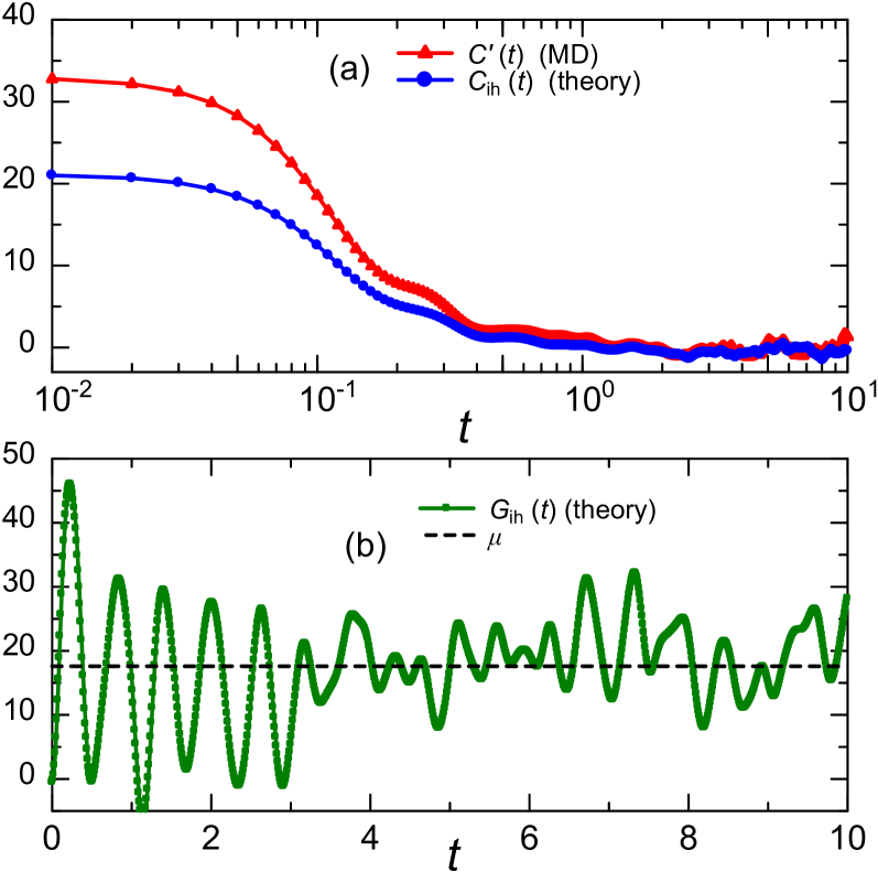
Figure 7: (Color online) (a) $C_{\rm ih}(t)$ in Eq.(79) and $C^{\prime}(t)\equiv[C(t)-C_{\rm pl}]/k_{B}T$ in Eq.(80) vs $t$ on a semi-logarithmic scale, where the former is from time-evolution of the eigenmodes and the latter is from molecular dynamics simulation at $T=0.01$. These decay on a timescale of 0.2. (b) $G_{\rm ih}(t)$ in Eqs.(34) and (81) vs $t$, which is zero at $t=0$, has a maximum ($\sim 47)$ at $t=0.23$, and exhibits complex oscillations around $\mu\cong 18$.

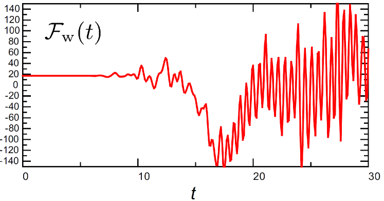
Figure 8: (Color online) Time-correlation function ${\cal F}_{\rm w}(t)$ in Eq.(82) for the forces from the walls to the particles as a function of $t$. At short times, it equal to $17$. For $t\gtrsim t_{\rm a}=H/c_{\perp}\cong 18$, it fluctuates irregularly due to scattering.

In Fig.7(a), we examine the stress time-correlation function at a fixed inherent state. We write it as

$$C_{\rm ih}(t)=\frac{\langle{\delta W_{\rm p}(t)\delta{W}_{\rm p}(0)}\rangle_{\rm ih}}{k_{B}TV}=\sum_{\lambda}\frac{(Z_{W}^{\lambda})^{2}}{V\omega_{\lambda}^{2}}{\cos(\omega_{\lambda}t)}.$$ (79)

In (a), this function decays to nearly zero on a rapid timescale of 0.2. Its oscillatory behavior is suppressed because of relatively small $Z_{W}^{\lambda}$ for not large $\lambda$ in Table 1, where the first term in Eq.(79) is $0.013\cos(\omega_{1}t)$. Notice that the large-scale sound modes do not contribute significantly to $\delta W_{\rm p}(t)$, because the difference $u_{ij}^{\alpha}=u_{i}^{\alpha}-u_{j}^{\alpha}$ appears for adjacent $i$ and $j$ in the first line of Eq.(25).

We also calculated the stress time-correlation function $C(t)$ in Eq.(61) at $T=0.01$ in a single run of molecular dynamic simulation with the same inherent state. Here, the time average was taken over the simulation time $t_{\rm sim}=5\times 10^{4}$. We used the stress integral $W(t)$ in Eq.(61) including the contributions from the bound particles, so there should be some boundary effect. Since Eq.(64) is predicted, Fig.7(a) gives

$$C^{\prime}(t)=[C(t)-C_{\rm pl}]/k_{B}T,$$ (80)

where $C_{\rm pl}=27.7$ is the plateau value. In (a), its initial value $C^{\prime}(0)=33.1$ is larger than $C_{\rm ih}(0)=21.2$, but the two curves fairly agree for $t\gtrsim 0.1$.

In Fig.7(b), we plot the stress relaxation function $G_{\rm ih}(t)$ in Eq.(34), which can be expressed as

$$G_{\rm ih}(t)=-\sum_{\lambda}\frac{Z_{W}^{\lambda}Z_{A}^{\lambda}}{V\omega_{\lambda}^{2}}\Big{[}{1-\cos(\omega_{\lambda}t)}\Big{]}.$$ (81)

In (b), this function exhibits complex oscillatory behavior with timescales shorter than $t_{\rm a}=c_{\perp}/H\sim 18$.

In Fig.8, we examine the time-correlation function of the forces from the walls. From Eq.(50), it is scaled as

$${\cal F}_{\rm w}(t)=\langle{\delta F_{\rm top}(t)\delta F_{\rm bot}(0)}\rangle_{\rm ih}H^{2}/Vk_{B}T.$$ (82)

This function can be expressed in the form of Eq.(59) from Eqs.(28) and (58). Starting with ${\cal F}_{\rm w}(0)=\mu\cong 17$. ${\cal F}_{\rm w}(t)$ is nearly constant for $t<t_{\rm a}\sim 18$. Around $t\sim t_{\rm a}$, the sound from the bottom is reflected in the reverse direction at the top, resulting in a large drop in $\delta F_{\rm top}(t)$. For $t\gtrsim t_{a}$, it largely fluctuates due to scattered waves. See Appendix B for ${\cal F}_{\rm w}(t)$ for homogeneous $\mu$.

From the argument below Eq.(50) we recognize that ${\cal F}_{\rm w}(t)$ in Eq.(82) is measurable experimentally. That is, at $t=0$, we move the bottom layer by $-H\gamma_{0}$ in a stepwise manner keeping the top layer at rest. Then, from Eq.(33), the average force from the top wall to the particles is given by $\gamma_{0}[{\cal F}_{\rm w}(0)-{\cal F}_{\rm w}(t)]$ per unit area at time $t(>0)$. As in Fig.8, it should vanish before arrival of the sounds.

Somfai et al.Roux calculated a force signal on a wall after emission of a pulse strain from the opposite wall in a granular model. Their signals without damping resemble ours in Fig.8, but they decay to zero with increasing viscous dissipation. Wittmer et al.Wit1 introduced friction in the stress relaxation in a random elastic network.

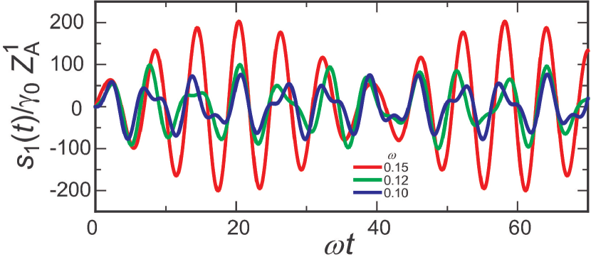
Figure 9: (Color online) Average time-evolution of the first-mode amplitude ${\bar{s}}_{1}(t)$ in Eq.(83) (divided by $\gamma_{0}Z_{A}^{1}$) after application of sinusoidal strain $\gamma_{\rm ex}(t)=\gamma_{0}\cos(\omega t)$ for $t>0$, where $\omega/\omega_{1}=0.1,0.12$, and 0.15.

IV.6 Resonance in periodic straining

We also suppose application of a sinusoidal strain $\gamma_{\rm ex}(t)=\gamma_{0}\theta(t)\sin(\omega t)$, which is zero for $t<0$. For $t>0$, substitution of this strain into Eq.(30) yields the average displacements ${\bar{u}}_{i}^{\alpha}(t)=\sum_{\lambda}e_{i\alpha}^{\lambda}{{\bar{s}_{\lambda}}(t)}/\sqrt{m_{i}}$. Here, ${{\bar{s}_{\lambda}}(t)}$ is the time-dependent average of the mode amplitude $s_{\lambda}(t)$ in Eq.(55). Then, ${{\bar{s}_{\lambda}}(t)}$ is a mixture of two oscillations,

$${{\bar{s}_{\lambda}}(t)}=\frac{{\gamma_{0}}Z_{A}^{\lambda}}{\omega_{\lambda}^{2}-\omega^{2}}\Big{[}\sin(\omega t)-\frac{\omega}{\omega_{\lambda}}\sin(\omega_{\lambda}t)\Big{]}\quad(t>0).$$ (83)

The term with the intrinsic frequency $\omega_{\lambda}$ remains nonvanishing, but it decays to zero in the presence of dissipation. Here, ${\bar{s}_{1}}(t)$ for the first mode grows as $(\omega_{1}^{2}-\omega^{2})^{-1}$ with increasing $\omega$ towards $\omega_{1}$. Thus, in Fig.9, ${\bar{s}_{1}}(t)$ is shown to increase with increasing $\omega$. However, as $\omega$ approaches $\omega_{1}$, the local strain increases near the walls and the linear theory becomes invalid,

The above displacement growth is a resonance effectLandau1 . Recently, we have performed a molecular dynamics simulation of a glass under periodic shearperiodic , where plastic events are proliferated at resonance frequencies. Wittmer et alWit1 studied resonance in a model network, where the growth is suppressed by the viscous friction.

V Summary and Remarks

In Sec.II, we have presented a linear response theory of applying a mean shear strain from boundary walls as in real experiments. Our theory is based on the relations (9) and (10) and is applicable to any solids and fluids in confined geometries. It can describe the linear dynamics in the bulk and near the boundary walls in terms of the appropriate time-correlation functions. It can be used even when the cell interior is inhomogeneous. As a first nontrivial application, this paper has mostly treated the linear response in glasses around a fixed inherent state.

In Sec.III, we have discussed the linear response in supercooled liquids with slow dynamics and in ordinary liquids with fast relaxations. In these states, the viscosity comes into play in the bulk. Our theory can further be used to study the boundary flow effects microscopically.

In Sec.IV, we have presented numerical results in a two-dimensional model glass on the basis of our theory. In Figs.3 and 4, the forces from the walls are correlated with the displacements of all the particles in the cell, resulting in heterogeneous responses. In Figs.5-9, time-dependent responses and time-correlation functions are strongly influenced by sound wave propagation and are very singular in glasses in the film geometry.

We make some remarks as follows.
(i) In real film systems, their temperature is regulated by heat transport between the walls and the interior particles. To realize this situation in molecular dynamics simulation, we can attach heat bathes to the boundary layers (not to the interior particles)Shiba . Sounds are then damped upon reflection at the walls, which leads to decays of the time-correlation functions.
(ii) Plastic events emit sounds leading to fast transport of the released potential energies throughout the system. Shiba and one of the present authorsShiba found that plastic events cause large oscillatory deviations in the force difference $F_{\rm top}^{x}(t)-F_{\rm bot}^{x}(t)$, where the heat bathes in the boundary layers damp such oscillations.
(iii) We can construct a microscopic theory of applying dilational strains by moving the walls along the $z$ axis, where propagation of the longitudinal sounds is crucial. In particular, the correlation between the normal components $\delta F_{\rm top}^{z}$ and $\delta F_{\rm bot}^{z}$ can be obtained if $\mu$ is replaced by $B+(2-2/d)\mu$ in Eq.(50), where $B$ is the bulk modulus.
(iv) In future, we should use a more realistic model of solid walls, where the forces from the particles in the walls to those in the cell are of great importanceslip . As discussed in Sec.IIIB, we can apply our theory to fluids to investigate the boundary flow profiles.
(v) There are a number of elastic systems with inhomogeneous elastic moduli on mesoscopic scalesHead ; Onukibook ; Hecke ; Luben ; Wit1 ; Bas , where nonaffine strains appear in applied stress. In gelsHead ; Onukibook , the crosslink structure is intrinsically random depending on the preparation condition. In multi-component metallic alloysOnukibook , the elasticity in the presence of precipitates is of great technological importance. which are harder or softer than the matrix.

$$U={\sum_{i}}^{\prime}\phi_{i}(d_{i})+\psi(d_{0})+\psi(d_{N}).$$ (A1)

The potentials $\phi_{i}(d_{i})$ can be random depending on $i$. Hereafter, we set ${\sum_{i}}^{\prime}=\sum_{1\leq i<N}$. The potential part of the microscopic pressure is of the form,

$$\Pi^{\rm p}(x)=-{\sum_{i}}^{\prime}\phi_{i}^{\prime}(d_{i})\theta_{i}(x),$$ (A2)

where $\phi_{i}^{\prime}(x)=d\phi_{i}(x)/dx$ and

$$\theta_{i}(x)={{\theta}}(x-x_{i})-\theta(x-x_{i+1}).$$ (A3)

Here, $\theta(x)$ is the step function equal to 1 for $x>0$ and to 0 for $x\leq 0$. Thus, $\theta_{i}(x)$ is 1 in the interval $x_{i}<x<x_{i+1}$ and is zero outside it. From Eq.(7) we find ${\hat{\delta}}(x,x_{i},x_{i+1})=\theta_{i}(x)/d_{i}$, leading to Eq.(A2).

At fixed $H=R_{N}-R_{1}$, we assume that the mechanical equilibrium holds at $x_{i}=x_{i}^{{\rm ih}}$ as

$$\phi^{\prime}_{i}(d_{i}^{\rm ih})=\psi^{\prime}(d_{0}^{\rm ih})=\psi^{\prime}(d_{N}^{\rm ih})\equiv-p_{\rm ih}.$$ (A4)

where $\psi^{\prime}(x)=d\psi(x)/dx$ and $d_{i}^{\rm ih}$, $d_{0}^{\rm ih}$, and $d_{N}^{\rm ih}(=d_{0}^{\rm ih})$ are the equilibrium values of $d_{i}$, $d_{0}$, and $d_{N}$, respectively. This state corresponds to the inherent state in glasses. From Eq.(A4) the potential part of the pressure is $\Pi^{\rm p}=p_{\rm ih}$ for $x_{1}^{\rm ih}<x<x_{N}^{\rm ih}$. We next consider small displacements $u_{i}=x_{i}-x_{i}^{\rm ih}$. At fixed $H$, the deviation of $U$ is bilinear in $u_{i}$ to leading order as

$$\delta U=\frac{1}{2}{\sum_{i}}^{\prime}{s_{i}}\xi_{i}^{2}+\frac{1}{2}{s_{0}}(u_{1}^{2}+u_{N}^{2}),$$ (A5)

where $\xi_{i}=d_{i}-d_{i}^{\rm ih}=u_{i+1}-u_{i}$, ${\sum_{i}}^{\prime}\xi_{i}=u_{N}-u_{1}$, and

$$s_{i}=\phi_{i}^{\prime\prime}(d_{i}^{\rm ih})\quad(1\leq i<N),\quad s_{0}=\psi^{\prime\prime}(d_{0}^{\rm ih}),$$ (A6)

with $\phi_{i}^{\prime\prime}(x)=d^{2}\phi_{i}(x)/dx^{2}$ and $\psi^{\prime\prime}(x)=d^{2}\psi(x)/dx^{2}$. We assume $s_{i}>0$ and $s_{0}>0$. At low $T$, $u_{i}$ fluctuate thermally obeying the Gaussian distribution $P_{\rm ih}\propto\exp(-\delta U/k_{B}T)$. Hereafter, $\langle{\cdots}\rangle_{\rm ih}$ denotes this average.

To linear order, the deviation of $\Pi^{\rm p}(x)$ is written as

$$\delta\Pi^{\rm p}(x) = -{\sum_{i}}^{\prime}s_{i}\xi_{i}\theta_{i}^{\rm ih}(x)$$ (A7)

$$-p_{\rm ih}[u_{N}\delta(x-x_{N}^{\rm ih})-u_{1}\delta(x-x_{1}^{\rm ih})],$$

where $\theta_{i}^{\rm ih}(x)=\theta(x-x_{i}^{\rm ih})-\theta(x,x_{i+1}^{\rm ih})$. The last term in Eq.(A7) vanishes in the range $x_{1}^{\rm ih}<x<x_{N}^{\rm ih}$. We then consider the correlation function for the thermal fluctuations of $\delta\Pi^{\rm p}$ defined by

$$C(x,x^{\prime})=\langle{\delta\Pi^{\rm p}(x)\delta\Pi^{\rm p}(x^{\prime})}\rangle_{\rm ih}/k_{B}T$$ (A8)

where $x$ and $x^{\prime}$ are in the range $[x_{1}^{\rm ih},x_{N}^{\rm ih}]$. Since $P_{\rm ih}$ is Gaussian, some calculations readily give

$${C(x,x^{\prime})}={\sum_{i}}^{\prime}s_{i}\theta_{i}^{\rm ih}(x)\theta_{i}^{\rm ih}(x^{\prime})-\frac{K}{H}.$$ (A9)

The first term is nonvanishing only when $x$ and $x^{\prime}$ are in the same interval, so it is short-ranged. The second term is a constant ($\propto H^{-1})$, which arises from the global elastic coupling. As will be shown in Eqs.(A14) and (A16), $K$ has the meaning of the elastic constant given by

$$K=H/[{\sum_{i}}^{\prime}s_{i}^{-1}+2s_{0}^{-1}]=[H/(N+1)]/\langle{s^{-1}}\rangle_{\rm ih},$$ (A10)

where $\langle{s^{-1}}\rangle_{\rm ih}$ is the average of $s_{i}^{-1}$ over all the bonds.

To derive Eq.(A9) we can use the variance relations,

$$\langle{\xi_{i}\xi_{j}}\rangle_{\rm ih}=c_{i}\delta_{ij}-c_{i}e_{j},~{}\langle{u_{1}^{2}}\rangle_{\rm ih}=\langle{u_{N}^{2}}\rangle_{\rm ih}=c_{0}-c_{0}e_{0},$$

$$\langle{\xi_{i}u_{N}}\rangle_{\rm ih}=-\langle{\xi_{i}u_{1}}\rangle_{\rm ih}=c_{i}e_{0},$$ (A11)

where $c_{i}=k_{B}T/s_{i}$ and $e_{i}=K/Hs_{i}$. We obtain the displacements from $u_{i}=u_{0}+\sum_{1\leq k<i}\xi_{k}$. ThusLuben ,

$$\langle{(u_{i}-u_{j})^{2}}\rangle_{\rm ih}/k_{B}T=\ell_{ij}-K\ell_{ij}^{2}/H,$$ (A12)

where $\ell_{ij}=\sum_{i\leq k<j}1/s_{k}$ for $i<j$. The two terms in Eq.(A12) grow with increasing $j-i$ but largely cancel for $\ell_{ij}>H/2K$. For $i=1$ and $j=N$, they nearly cancel as $\langle{(u_{N}-u_{1})^{2}}\rangle_{\rm ih}/k_{B}T=2(1-2e_{0})/s_{0}$. We also find the counterpart of Eq.(50) in the form,

$$s_{0}^{2}\langle{u_{1}u_{N}}\rangle_{\rm ih}/k_{B}T=K/H.$$ (A13)

Next, we shift the top as $R_{N}\to R_{N}+\delta R_{N}$ keeping the bottom at rest with mean strain $\epsilon_{\rm ex}=\delta R_{N}/H$. The potential energy $U$ changes by $-p_{\rm ih}\delta R_{N}+\delta U^{\prime}$ with

$$\delta U^{\prime}=\frac{1}{2}{\sum_{i}}^{\prime}{s_{i}}{\xi_{i}^{2}}+\frac{1}{2}{s_{0}}u_{1}^{2}+\frac{1}{2}{s_{0}}(u_{N}-\delta R_{N})^{2}$$

$$=K\epsilon_{\rm ex}^{2}H/2,$$ (A14)

which corresponds to Eq.(46). Minimization of the first line of Eq.(A14) yields shifts of the particle positions given by $\xi_{i}=K{\epsilon_{\rm ex}}/{s_{i}}$, $u_{1}=\delta R_{N}-u_{N}=K{\epsilon_{\rm ex}}/{s_{0}}$, for which we obtain the second line.

We also use the linear response theoryKubo for a small strain. The perturbed Hamiltonian is ${\cal H}_{\rm ih}^{\prime}=\sum_{i}|{\mbox{\boldmath$p$}}_{i}|^{2}/2m_{i}+\delta U-\epsilon_{\rm ex}\delta{\cal A}$, where the first term is the kinetic energy, $\delta U$ is given by Eq.(A5), and

$$\delta{\cal A}=\frac{s_{0}}{2}H(u_{N}-u_{1})=\int d{x}\delta\Pi^{\rm p}-\sum_{i}x_{i}^{\rm ih}f_{i},$$ (A15)

where $f_{i}=-\partial(\delta U)/\partial u_{i}$. As in Eq.(38) we obtain

$$K=-\int dx\langle{\delta\Pi^{\rm p}(x)\delta{\cal A}}\rangle_{\rm ih}/Hk_{B}T=K_{\rm a}-K_{\rm c}.$$ (A16)

From Eq.(A15), $K_{\rm a}$ is the affine part and $K_{\rm c}$ is the nonaffine part. From Eqs.(A7) and (A8) we find

$$K_{\rm a}=-{\sum_{i}}^{\prime}\frac{x_{i}^{\rm ih}}{H}\frac{\partial}{\partial u_{i}}\int dx\delta\Pi^{\rm p}=\frac{1}{H}{\sum_{i}}^{\prime}s_{i}(d_{i}^{\rm ih})^{2},$$ (A17)

$$K_{\rm c}=\frac{1}{H}\int dx\int dx^{\prime}{C(x,x^{\prime})}=K_{\rm a}-K.$$ (A18)

In $K_{\rm c}$, the first and second terms in Eq.(A9) yield $K_{\rm a}$ and $-K$, respectively, after double integration.

We notice that, if some bonds are very weak (with very small $s_{i}$), they can dominantly contribute to $\langle{s^{-1}}\rangle_{\rm ih}$ giving rise to a large reduction in $K$. In such cases, $K$ can be much smaller than $K_{\rm a}$.

Appendix B: Thermal fluctuations in solid films in continuum elasticity

In the linear elasticity, we consider a solid film with homogeneous elastic moduli, where the displacement field ${\mbox{\boldmath$u$}}({\mbox{\boldmath$r$}})$ is well-defined. We assume that the thermal fluctuations of $u$ obey the distribution $\propto\exp(-F_{\rm el}/k_{B}T)$, where $F_{\rm el}$ is the elastic free energyGusev ; Binder ; Rahman . Here, the average over this distribution is written as $\langle{\cdots}\rangle$. We impose the rigid boundary condition at $z=\pm H/2$ and the periodic boundary condition along the $x$ and $y$ axes with period $L$. The film volume is $V=HS$ with $S=L^{d-1}$. .

First, we examine the equal-time correlations. For simplicity, we consider the lateral average of $u_{x}$ (the zero wavenumber component in the $x$-$y$ plane) given by

$$U_{x}(z)=S^{-1}\int d{\mbox{\boldmath$r$}}_{\perp}u_{x}({\mbox{\boldmath$r$}}),$$ (B1)

where $\int d{\mbox{\boldmath$r$}}_{\perp}$ is the integral in the $x$-$y$ plane. The normalized eigenfunctions are $e_{n}(z)=\sqrt{2/V}\sin[k_{n}(z+H/2)]$ $(n\geq 1$) with $k_{n}=\pi n/H$ for $U_{x}(\pm H/2)=0$. As in Eq.(55), we introduce the fluctuating variables $s_{n}$ by

$$U_{x}(z)=\sum_{n\geq 1}e_{n}(z)s_{n}.$$ (B2)

As in Eq.(57), the elastic free energy is expressed as

$$F_{\rm el}=\frac{1}{2}\mu S\int dz(U_{x}^{\prime})^{2}=\frac{1}{2}\mu\sum_{n\geq 1}k_{n}^{2}s_{n}^{2},$$ (B3)

where $\mu$ is the shear modulus and $U_{x}^{\prime}(z)=dU_{x}(z)/dz$. Then, we find $\langle{s_{n}s_{\ell}}\rangle=k_{B}T\delta_{n\ell}/\mu k_{n}^{2}$ and

$$\langle{U_{x}(z)U_{x}(z^{\prime})}\rangle/{k_{B}T}=\sum_{n\geq 1}e_{n}(z)e_{n}(z^{\prime})/{\mu k_{n}^{2}}$$

$$\hskip 19.91684pt=[{H^{2}}-2{H}|z-z^{\prime}|-4zz^{\prime}]/{4\mu V},$$ (B4)

where we use the formula $\sum_{n\geq 1}\sin(np)\sin(nq)/n^{2}=q(\pi-p)/2$ for $0<q<p<\pi$. Differentiation of Eq.(B4) with respect to $z$ and $z^{\prime}$ gives the strain correlation,

$$\langle{U_{x}^{\prime}(z)U_{x}^{\prime}(z^{\prime})}\rangle/{k_{B}T}=[H\delta(z-z^{\prime})-1]/\mu V.$$ (B5)

Here, the $\delta$-function appears, but it should be regarded as a function with a microscopic width in particle systems.

In Eq.(28) we have introduced the forces from the walls. In the continuum theory, we express them as

$${\delta F_{\rm top}^{x}}={S}\mu U_{x}^{\prime}({H^{\prime}}/{2}),\quad{\delta F_{\rm bot}^{x}}=-{S}\mu U_{x}^{\prime}(-H^{\prime}/2).$$ (B6)

To account for the particle discreteness, we assume the stress balance at $z=\pm H^{\prime}/2$, where $H^{\prime}=H-\ell_{\rm m}$ with $\ell_{\rm m}$ being a microscopic length. For $|z|<H^{\prime}/2$, we find $\langle{U_{x}(z)\delta F_{\rm top}^{x}}\rangle/k_{B}T=-z/H-1/2$ and $\langle{U_{x}(z)\delta F_{\rm bot}^{x}}\rangle/k_{B}T=z/H-1/2$ from Eq.(B4). These lead to the counterparts of Eqs.(35) and (47). If we define $\delta{\cal A}=H(\delta F_{\rm bot}^{x}-\delta F_{\rm top}^{x})/2$ as in Eq.(27), we find

$$\langle{U_{x}(z)\delta{\cal A}}\rangle/k_{B}T=z,$$ (B7)

which consists of the affine displacement only. To be precise, $\langle{U_{x}(z)\delta{\cal A}}\rangle$ nearly vanishes in the narrow layers $H^{\prime}/2<|z|<H/2$. If we assume the linear combination $\delta{\cal A}=\sum_{n}Z_{A}^{(n)}s_{n}$ in terms of $s_{n}$ in Eq.(B2), the coefficients $Z_{A}^{(n)}$ are nonvanishing only for even positive $n$ as

$$Z_{A}^{(n)}=-2\pi(\sqrt{2V}/H)\mu n\quad({n=2,4,\dots}).$$ (B8)

Next, we examine the time-correlations assuming the wave equation $\partial^{2}U_{x}/\partial t^{2}=c_{\perp}^{2}\partial^{2}U_{x}/\partial z^{2}$ without dissipation, where $c_{\perp}$ is the transverse sound speed. Fixing $z^{\prime}$ in the cell $|z^{\prime}|<H/2$, we have

$$\langle{U_{x}(z,t)U_{x}(z^{\prime},0)}\rangle=g(z+c_{\perp}t,z^{\prime})+g(z-c_{\perp}t,z^{\prime}),$$ (B9)

where $2g(z,z^{\prime})$ is equal to Eq.(B4) for $|z|<H/2$. We extend it outside the cell setting $g(z,z^{\prime})=-g(H-z,z^{\prime})=g(z+2H,z^{\prime})$. We can obtain Eq.(B9) if we replace $e_{n}(z)e_{n}(z^{\prime})$ by $e_{n}(z)e_{n}(z^{\prime})\cos(c_{\perp}k_{n}t)$ in the first line of Eq.(B4). Then, Eq.(B9) gives a periodic function of $t$ and the period is twice larger than the acoustic traversal time $t_{\rm a}=H/c_{\perp}$. From Eqs.(B6) and (B9), the function ${\cal F}_{\rm w}(t)$ defined in Eq.(82) is calculated as

$${\cal F}_{\rm w}(t)=\mu-\mu\sum_{\ell=0,\pm 1,\pm 2,\cdots}\delta(t/t_{\rm a}-1-2\ell),$$ (B10)

where the second term arises from impulses due to repeated reflections of transverse sounds without scattering. Thus, Eq.(B10) is consistent with Fig.8 for $t<t_{\rm a}$.

References

- (1) K. Maeda and S. Takeuchi, “Atomistic process of plastic deformation in a model amorphous metal,” Philos. Mag. A 44, 643 (1981).
- (2) R. Yamamoto and A. Onuki, “Dynamics of highly supercooled liquids: Heterogeneity, rheology, and diffusion,” Phys. Rev. E 58, 3515-3529 (1998).
- (3) D. L. Malandro and D. J. Lacks, “Relationships of shear-induced changes in the potential energy landscape to the mechanical properties of ductile glasses,” J. Chem. Phys. 110, 4593 (1999)
- (4) C. Maloney and A. Lemaître, “Amorphous systems in athermal, quasistatic shear,” Phys. Rev. E 74, 016118 (2006).
- (5) M. Tsamados, A. Tanguy, C. Goldenberg, and J.-L. Barrat, “Local elasticity map and plasticity in a model Lennard-Jones glass,” Phys. Rev. E 80, 026112 (2009).
- (6) M. L. Manning and J. Liu, “Vibrational modes identify soft spots in a sheared disordered packing,” Phys. Rev. Lett. 107, 108302 (2011).
- (7) T. Kawasaki and A. Onuki, “Slow relaxations and stringlike jump motions in fragile glass-forming liquids: Breakdown of the Stokes-Einstein relation,” Phys. Rev. E 87, 012312 (2013).
- (8) D. R. Squire, A. C. Holt, and W. G. Hoover, “Isothermal elastic constants for argon. Theory and Monte Carlo calculations,” Physica (Amsterdam) 42, 388 (1969).
- (9) J. R. Ray, “Elastic constants and statistical ensembles in molecular dynamics,” Comput. Phys. Rep. 8, 109-151 (1988).
- (10) J. F. Lutsko, “Generalized expressions for the calculation of elastic constants by computer simulation,” J. Appl. Phys. 65, 2991 (1989).
- (11) S. Hess, M. Krger, and W. G. Hoover, “Shear modulus of fluids and solids,” Physica A 239, 449-466 (1997).
- (12) K. Yoshimoto, G. J. Papakonstantopoulos, J. F. Lutsko, and J. J. de Pablo, “Statistical calculation of elastic moduli for atomistic models,” Phys. Rev. B 71, 184108 (2005).
- (13) M. Parrinello and A. Rahman, “Strain fluctuations and elastic constants,” J. Chem. Phys. 76, 2662-2666 (1982).
- (14) A. A. Gusev, M. M. Zehnder, and U. W. Suter, “Fluctuation formula for elastic constants,” Phys. Rev. B 54, 1 (1996).
- (15) S. Sengupta, P. Nielaba, M. Rao, and K. Binder, “Elastic constants from microscopic strain fluctuations,” Phys. Rrev. E 61, 1072-1080 (2000).
- (16) C. Maloney and A. Lemaître, “Universal Breakdown of Elasticity at the Onset of Material Failure,” Phys. Rev. Lett. 93, 195501 (2004).
- (17) A. Lemaître and C. Maloney, “Sum rules for the quasi-static and visco-elastic response of disordered solids at zero temperature,” J. Stat. Phys. 123, 415-453 (2006).
- (18) S. R.Williams and D. J. Evans, “The rheology of solid glass,” J. Chem. Phys. 132, 184105 (2010).
- (19) S. R. Williams, “Communication: Broken-ergodicity and the emergence of solid behaviour in amorphous materials,” J. Chem. Phys. 135, 131102 (2011).
- (20) H. Yoshino, “Replica theory of the rigidity of structural glasses, h J. Chem. Phys. 136, 214108 (2012).
- (21) A. Tanguy, J.P. Wittmer, F. Leonforte, J.-L. Barrat, “Continuum limit of amorphous elastic bodies: A finite-size study of low-frequency harmonic vibrations,” Phys. Rev. B 66, 174205 (2002).
- (22) H. Mizuno, S. Mossa, and J-L. Barrat, “ Measuring spatial distribution of the local elastic modulus in glasses Phys. Rev. E 87, 042306 (2013).
- (23) A. Zaccone and E. Scossa-Romano, “Approximate analytical description of the nonaffine response of amorphous solids,” Phys. Rev. B 83, 184205 (2011).
- (24) A. Zaccone and E. M. Terentjev, “Disorder-assisted melting and the glass transition in amorphous solids,” Phys. Rev. Lett. 110, 178002 (2013).
- (25) J. P. Wittmer, H. Xu, P. Poliska, F. Weysser, and J. Baschnagel, “Shear modulus of simulated glass-forming model systems: Effects of boundary condition, temperature, and sampling time,” J. Chem. Phys. 138, 12A533 (2013).
- (26) J.P. Wittmer, H. Xu, O. Benzerara, and J. Baschnagel, “Fluctuation-dissipation relation between shear stress relaxation modulus and shear stress autocorrelation function revisited,” Molecular Physics, 113, 2881-2893 (2015).
- (27) I. Fuereder and P. Ilg, “Influence of inherent structure shear stress of supercooled liquids on their shear moduli,” J. Chem. Phys. 142, 144505 (2015).
- (28) S. Saw and P. Harrowell, “Rigidity in Condensed Matter and Its Origin in Configurational Constraint”, Phys. Rev. Lett. 116, 137801 (2016).
- (29) K. Yoshimoto, T. S. Jain, K. Van Workum, P. F. Nealey, and J. J. de Pablo, “Mechanical heterogeneities in model polymer glasses at small length scales,” Phys. Rev. Lett. 93, 175501 (2004).
- (30) H. Mizuno, L. E. Silbert, and M. Sperl, “Spatial distributions of local elastic moduli near the jamming transition,” Phys. Rev. Lett. 116, 068302 (2016).
- (31) S. Sastry, P. G. Debenedetti, and F. H. Stillinger, “Signatures of distinct dynamical regimes in the energy landscape of a glass-forming liquid,” Nature 393, 554-557 (1998).
- (32) A. Heuer, “Exploring the potential energy landscape of glass-forming systems: From inherent structures via metabasins to macroscopic transport,” J. Phys.: Condens. Matter 20, 373101 (2008).
- (33) S. Abraham and P. Harrowell, “The origin of persistent shear stress in supercooled liquids,” J. Chem. Phys. 137, 014506 (2012).
- (34) S. Chowdhury, S. Abraham, T. Hudson, and P. Harrowell, “Long range stress correlations in the inherent structures of liquids at Rest,” J. Chem. Phys. 144, 124508 (2016).
- (35) R. Zwanzig, “Time-correlation functions and transport coefficients in statistical mechanics,” Annu. Rev. Phys. Chem. 16, 67-101 (1965).
- (36) J.-P. Hansen and I. R. Mcdonald, Theory of Simple Liquids (Academic, 2006).
- (37) A. Onuki, Phase Transition Dynamics (Cambridge University Press, Cambridge, 2002).
- (38) L. Onsager, “Reciprocal relations in irreversible processes.I.,” Phys. Rev. 37, 405-426 (1931).
- (39) M.S. Green, “Markoff random processes and the statistical mechanics of time-dpendent phenomena. II. Irreversible processes in fluids,” J. Chem. Phys. 22, 398-413 (1954).
- (40) L.P. Kadanoff and P.C. Martin, “Hydrodynamic Equations and Correlation Functions,” Annals of Physics 24, 419-469 (1963)
- (41) R. Kubo, “Statistical-mechanical theory of irreversible processes.I. General theory and simple applications to magnetic and conduction problems,” J. Phys. Soc. Jpn. 12, 570-586 (1957).
- (42) L. Bocquet and J. -L. Barrat, “Flow boundary conditions from nano- to micro-scales,” Soft Matter 3, 685-693 (2007).
- (43) V. A. Levashov, J. R. Morris, and T. Egami, “Anisotropic stress correlations in two-dimensional liquids,” Phys. Rev. Lett. 106, 115703 (2011).
- (44) A. Lemaître, “Structural relaxation is a scale-free process,” Phys. Rev. Lett. 113, 245702 (2014).
- (45) M. Maier, A. Zippelius and M. Fuchs, “Emergence of Long-Ranged Stress Correlations at the Liquid to Glass Transition,” Phys. Rev. Lett. 119, 265701 (2017).
- (46) L. Klochko, J. Baschnagel, J. P. Wittmer and A. N. Semenov, “Long-range stress correlations in viscoelastic and glass-forming fluids,” Soft Matter, 14, 6835 (2018).
- (47) B. U. Felderhof, “Fluctuations of polarization and magnetization in dielectric and magnetic media,” J. Chem. Phys. 67, 493-500 (1977).
- (48) K. Takae and A. Onuki, “Fluctuations of local electric field and dipole moments in water between metal walls,” J. Chem. Phys. 143, 154503 (2015).
- (49) X. Jia, C. Caroli, and B. Velicky, “Ultrasound Propagation in Externally Stressed Granular Media,” Phys. Rev. Lett. 82, 1863 (1999).
- (50) E. Somfai, J.-N. Roux, J. H. Snoeijer, M. van Hecke, and W.van Saarloos, “Elastic wave propagation in confined granular systems,” Phys. Rev. E 72, 021301 (2005).
- (51) H. Shiba and A. Onuki, “Plastic deformations in crystal, polycrystal, and glass in binary mixtures under shear: collective yielding, ” Phys. Rev. E 81, 051501 (2010); “Jammed particle configurations and dynamics in high-density Lennard-Jones binary mixtures in two dimensions,” Prog. Theor. Phys. Suppl. No. 184, 234 (2010).
- (52) J. H. Irving and J. G. Kirkwood, “The statistical mechanical theory of transport processes. IV. The equations of hydrodynamics.” J. Chem. Phys. 18, 817-829 (1949).
- (53) H. R. Schober and G. Ruocco, “Size effects and quasilocalized vibrations,” Philosophical Magazine, 84, 1361-1372 (2006).
- (54) Y. Matsuoka, H. Mizuno, and R. Yamamoto, “Acoustic wave propagation through a supercooled liquid: A normal mode analysis,” J. Phys. Soc. Jpn. 81, 124602 (6 pages) (2012).
- (55) S. N. Taraskin and S. R. Elliott, “Propagation of plane-wave vibrational excitations in disordered systems,” Phys. Rev. B 61, 12017-12029 (2000).
- (56) S. Gelin, H. Tanaka, and A. Lemaître, “Anomalous phonon scattering and elastic correlations in amorphous solids,” Nature Materials 15, 1177-1181 (2016).
- (57) M. Doi and S. F. Edwards, The Theory of Polymer Dy- namics (Clarendon Press, Oxford, 1986).
- (58) R. Zwanzig and R. D. Mountain, “High-Frequency Elastic Moduli of Simple Fluids,” J. Chem. Phys. 43, 4464-4471 (1965).
- (59) A. Kushima, X. Lin, J. Li, J. Eapen, J.C. Mauro, X. Qian, P. Diep, and S. Yip, “Computing the viscosity of supercooled liquids,” J. Chem. Phys. 130, 224504 (2009).
- (60) L.D. Landau and E.M. Lifshitz, Mechanics (Pergamon, New York,1969).
- (61) T. Kawasaki and A. Onuki, “Acoustic resonance in periodically sheared glass,” arXiv:1708.03166.
- (62) J. Bastide and L. Leibler, “Large-scale heterogeneities in randomly cross-linked networks,” Macromolecules 21, 2647 (1988).
- (63) D. A. Head, A. J. Levine, and E. C. MacKintosh, “Deformation of Cross-Linked Semiflexible Polymer Networks,” Phys. Rev.Lett. 91, 108102 (2003).
- (64) B.A. DiDonna and T.C. Lubensky, “Nonaffine correlations in random elastic media,” Phys. Rev. E 72, 066619 (2005).
- (65) W. G. Ellenbroek, Z. Zeravcic, W. van Saarloos, and M. van Hecke, “Non-affine response: Jammed packings vs. spring networks,” Europhys. Lett. 87, 34004 (2009).