Super-universality of eigenchannel structures and possible optical applications

Abstract

The propagation of waves through transmission eigenchannels in complex media is emerging as a new frontier of condensed matter and wave physics. A crucial step towards constructing a complete theory of eigenchannels is to demonstrate their spatial structure in any dimension and their wave-coherence nature. Here, we show a surprising result in this direction. Specifically, we find that as the width of diffusive samples increases transforming from quasi one-dimensional ($1$D) to two-dimensional ($2$D) geometry, notwithstanding the dramatic changes in the transverse (with respect to the direction of propagation) intensity distribution of waves propagating in such channels, the dependence of intensity on the longitudinal coordinate does not change and is given by the same analytical expression as that for quasi-$1$D. Furthermore, with a minimal modification, the expression describes also the spatial structures of localized resonances in strictly $1$D random systems. It is thus suggested that the underlying physics of eigenchannels might include super-universal key ingredients: they are not only universal with respect to the disorder ensemble and the dimension, but also of $1$D nature and closely related to the resonances. Our findings open up a way to tailor the spatial energy density distribution in opaque materials.

I Introduction

An unprecedented degree of control reached in experiments on classical waves is turning the dream of understanding and controlling wave propagation in complex media into reality Rotter17 . Central to many ongoing research activities is the concept of transmission eigenchannel Mosk08 ; Choi12 ; Choi11 ; Mosk12 ; Genack12 ; Tian15 ; Cao15 ; Lagendijk16 ; Cao16 ; Yamilov16 ; Yilmaz16 ; Cao17 ; Lagendijk18 ; Cao18 ; Tian18 (abbreviated as eigenchannel herefater). Loosely speaking, the eigenchannel refers to a specific wave field, which is excited by the input waveform corresponding to the right-singular vector Dorokhov82 ; Dorokhov84 ; Mello88 of the transmission matrix (TM) $\bm{t}$. When a wave is launched into a complex medium it is decomposed into a number of “partial waves”, each of which propagates along an eigenchannel and whose superposition gives the field distribution excited by the incoming wave. Thus, in contrast to the TM, which treats media as a black box and has been well studied Beenakker97 , eigenchannels are much less explored, in spite of the fact that these provide rich information about the properties of wave propagation in the interior of the media. The understanding of the spatial structures of these channels can provide a basis for both fundamentals and applications of wave physics in complex media.

So far, the emphasis has been placed on the structures of eigenchannels in quasi $1$D disordered media Genack12 ; Tian15 ; Cao15 ; Lagendijk16 ; Cao16 ; Yamilov16 . Yet, measurements of the high-dimensional spatial resolution of eigenchannels have been within experimental reach very recently Lagendijk18 ; Cao18 . An intriguing localization structure of eigenchannels in the transverse direction has been observed in both real and numerical experiments for a very wide $2$D diffusive slab Cao18 ; Tian18 . In addition, numerical results Tian18 have suggested that in this kind of special high-dimensional media, even in a single disorder configuration, the eigenchannel structure can carry some universalities that embrace quasi $1$D eigenchannels as well. Here we study the evolution of the eigenchannels in the crossover from low to higher dimension, which so far has not been explored. This not only provides a new angle for the fundamentals of wave propagation in disordered media, but is practically important for both experiments and applications of the eigenchannel structure in higher dimension.

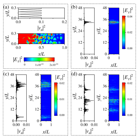
Figure 1: Simulations show that as the width $W$ increases, so that a quasi-$1$D ($N=5$) waveguide turns into a $2$D slab ($N=800$), the eigenchannel structure $|E_{\tau}(x,y)|^{2}$ in a single disordered medium undergoes dramatic changes in the transverse $y$ direction. For $N=5$, the transverse structure is always declocalized (a). For $N=800$, the transverse structure exhibits very rich localization behaviors for fixed disorder configuration: for example, the structure exhibits one, two and three localization peaks in (b), (c) and (d), respectively. Moreover, the transverse structures of eigenchannels are qualitatively the same as the structures of $|v_{n}(y)|^{2}$. For all panels, the eigenvalue $\tau\approx 0.6$ and $L=50$.

Another motivation of the present work comes from a recent surprising finding Bliokh15 regarding a seemingly unrelated object, the resonance in layered disordered samples which, from the mathematical point of view, are strictly $1$D systems. The resonance refers to a local maximum in the transmittance spectrum Freilikher04 , which has a natural connection to Anderson localization in $1$D Anderson58 ; Gershenshtein59 and resonators in various systems, ranging from plasmonics to metamaterials Freilikher03 . Despite the conceptual difference between the resonance and the eigenchannel, it was found Bliokh15 that the distribution of resonant transmissions in the (i) $1$D Anderson localized regime and (ii) the transmission eigenvalues in quasi-$1$D diffusive regime are exactly the same, namely, the bimodal distribution Dorokhov82 ; Mello88 . However, the mechanism underlying this similarity remains unclear. It is of fundamental interest to understand whether this similarity is restricted only to transmissions, or can be extended to spatial structures.

In this work we show that in a diffusive medium, as the width of a sample (and consequently the number of channels) increases so that the sample crosses over from quasi $1$D to higher dimension, eigenchannels exhibit transverse structures much richer than what were found previously Cao18 ; Tian18 . In particular, given a disorder configuration, not only can we see the previously found Cao18 ; Tian18 localization structure, but also a necklace like structure which is composed of several localization peaks. Most surprisingly, notwithstanding the appearance of such diverse transverse structures in the dimension crossover, the longitudinal structure of eigenchannels, namely, the depth profile of the energy density (integrated over the cross section), remains unaffected, and is given by precisely the same expression as that for quasi-$1$D found in Ref. Tian15, . We also study the spatial structures of resonance in strictly $1$D. We find that they have a universal analytic expression, which is similar to that for eigenchannel structures, and the modification is minimal. Our findings may serve as a proof of the conjecture Choi11 of the eigenchannel structure–Fabry-Perot cavity analogy.

The remainder of this paper is organized as follows. In Sec. II, we introduce some basic concepts of eigenchannels and resonances. In Sec. III, we study in detail how the eigenchannel structure in a diffusive medium evolves as the medium crosses over from quasi-$1$D to a higher-dimensional slab geometry. To be specific, throughout this work we focus on $2$D samples. In Sec. IV, we study in detail the spatial structure of $1$D resonances. In Sec. V, possible optical applications are discussed. In Sec. VI, we conclude and discuss the results.

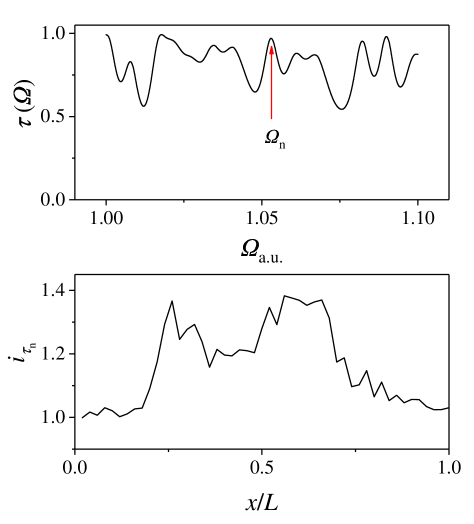
Figure 2: Example of a transmittance spectrum $\mathcal{T}(\Omega)$ (top) and the resonance structure ${\tilde{I}}_{\mathcal{T}_{n}}(x)$ corresponding to the resonant frequency $\Omega_{n}$ (bottom).

II Eigenchannel and resonance: basic concepts

To introduce the concept of eigenchannels Rotter17 ; Choi11 ; Tian15 , we consider the transmission of a monochromatic wave (with circular frequency $\Omega$) through a rectangular ($0\leq x\leq L,0\leq y\leq W$) diffusive dielectric medium bounded in the transverse ($y$) direction by reflecting walls at $y=0$ and $y=W$. For $W\gtrsim L$ ($W\ll L$) the medium geometry is $2$D (quasi $1$D). The wave field $E(x,y)$ satisfies the Helmholtz equation, (the velocity of waves in the background is set to unity.)

$$\left\{\partial_{x}^{2}+\partial_{y}^{2}+\Omega^{2}\left[1+\delta\epsilon(x,y)\right]\right\}E(x,y)=0,$$ (1)

where $\delta\epsilon(x,y)$ is a random function, which presents the fluctuations of the dielectric constant inside the sample, and equals zero at $x<0$ and $x>L$. To study the evolution of the eigenchannel structure in the crossover from quasi-$1$D to $2$D, we increase $W$ and keep $L$, $\Omega$ and the strength of disorder fixed.

The incoming and transmitted current amplitudes are related to each other by the transmission matrix $\bm{t}\equiv\{t_{ab}\}$, where $a,b$ label the ideal [i.e., $\delta\epsilon(x,y)=0$] waveguide modes $\varphi_{a}(y)$. The matrix elements are

$$t_{ab}=-i\sqrt{\tilde{v}_{a}\tilde{v}_{b}}\;\langle x=L,a|G|x^{\prime}=0,b\rangle,$$ (2)

where $G$ is the retarded Green’s function associated with Eq. (1), and $\tilde{v}_{a}$ is the group velocity of mode $a$.

Since the matrix $\bm{t}$ is non-hermitian, we perform its singular value decomposition, i.e., $\bm{t}=\sum_{n=1}^{N}\bm{u}_{n}\sqrt{\tau_{n}}\bm{v}_{n}^{\dagger}$ to find the singular value $\sqrt{\tau_{n}}$ and the corresponding left (right)-singular vector $\bm{v}_{n}$ ($\bm{u}_{n}$) normalized to unity. The input waveform $\bm{v}_{n}$ uniquely determines the $n$th eigenchannel, over which radiation propagates in a random medium Rotter17 ; Choi11 ; Tian15 , and $\tau_{n}$ gives the transmission coefficient of the $n$th eigenchannel and is also called the transmission eigenvalue. The total transmittance is given by $\sum_{n}\tau_{n}$. Moreover, many statistical properties of transport through random media such as the fluctuations and correlations of conductance and transmission may be described in terms of the statistics of $\tau_{n}$ Tian15 .

To find the spatial structure of eigenchannels, we replace $x=L$ in Eq. (2) by arbitrary $x\in[0,L)$, i.e.,

$$t_{ab}\rightarrow t_{ab}(x)\equiv-i\sqrt{\tilde{v}_{a}\tilde{v}_{b}}\;\langle x,a|G|x^{\prime}=0,b\rangle.$$ (3)

This gives the field distribution inside the medium,

$$\bm{E}_{\tau_{n}}(x)\equiv\{E_{na}(x)\}=\bm{t}(x)\bm{v}_{n},$$ (4)

excited by the input field $\bm{v}_{n}$. Changing from the ideal waveguide mode ($\varphi_{a}$) representation to the coordinate $(x,y)$ representation gives a specific $2$D spatial structure, namely, the energy density profile:

$$|\bm{E}_{\tau_{n}}(x,y)|^{2}=\left|\sum_{a=1}^{N}E_{na}(x)\varphi_{a}^{*}(y)\right|^{2},$$ (5)

which defines the $2$D eigenchannel structure associated with the transmission eigenvalue $\tau_{n}$. Examples of this $2$D structure are given in Fig. 1. Integrating Eq. (5) over the transverse coordinate $y$ we obtain the depth profile of the energy density of the $n$th eigenchannel,

$$w_{\tau_{n}}(x)\equiv\int dy|\bm{E}_{\tau_{n}}(x,y)|^{2},$$ (6)

a key quantity to be addressed below. Note that, in the definitions of (5) and (6), the frequency $\Omega$ is fixed.

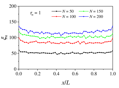
Figure 3: Simulation results of the $x$-dependent participation ratio $\xi_{n}(x)$ for different values of $N$.

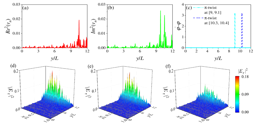
Figure 4: A numerical example shows that $v_{n}(y)$ (high transmission) is localized approximately in the region of $9\leq y/L\leq 12$ (a,b). This localization of $v_{n}(y)$ at the input edge leads to the localization of eigenchannel structure in the $y$ direction in the interior of the medium (d). When the phase of $v_{n}(y)$ in the region of $9.0\leq y/L\leq 9.1$ is twisted by $\pi$ (c, dotted-dashed line), the eigenchannel structure is unaffected (e). Whereas if the $\pi$-phase twist is introduced in the region of $10.3\leq y/L\leq 10.4$ (c, dashed line), the eigenchannel structure is significantly changed (f). $N=200$.

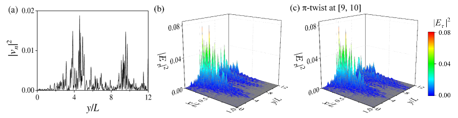
Figure 5: A numerical example shows that $v_{n}(y)$ (low transmission, $\tau_{n}=0.009$) exhibits two localization peaks, which are located approximately in the region of $3\leq y/L\leq 5$ and $9\leq y/L\leq 11$, respectively (a). This necklace state-like structure of $v_{n}(y)$ at the input edge leads to two localization peaks of eigenchannel structure in the $y$ direction in the interior of the medium (b). When the phase of $v_{n}(y)$ in the region of $9\leq y/L\leq 10$ is twisted by $\pi$, the localization peak of the eigenchannel structure corresponding to the localization region $9\leq y/L\leq 11$ of $v_{n}(y)$ is significantly changed, whereas the other peak corresponding to the localization region $3\leq y/L\leq 5$ of $v_{n}(y)$ is unaffected (c). $N=200$.

To proceed, we present a brief review of resonances in media with $1$D disorder (cf. Fig. 2). For a detailed introduction we refer to Ref. Freilikher03, . In the strictly $1$D case, the wave field $E_{\Omega}(x)$ satisfies

$$\left\{\partial_{x}^{2}+\Omega^{2}\left[1+\delta\epsilon(x)\right]\right\}E_{\Omega}(x)=0,$$ (7)

where $\delta\epsilon(x)$ represents the fluctuation of the dielectric constant, and like Eq. (1) the wave velocity at the background is set to unity. For each solution of Eq. (7) with a given $\Omega$ there is a specific transmittance $\mathcal{T}(\Omega)$. We define the resonance as a local maximum $\mathcal{T}(\Omega_{n})\equiv\mathcal{T}_{n}$ of the transmittance spectrum $\{\mathcal{T}(\Omega)\}$, where $\Omega_{n}$ is the resonant frequency. The energy density of the field at the resonant frequency is defined as the resonance structure:

$${\tilde{I}}_{\mathcal{T}_{n}}(x)\equiv|E_{\Omega_{n}}(x)|^{2},$$ (8)

another key quantity to be addressed below. Importantly, contrary to the eigenchannel structure, Eq. (5), where $\Omega$ is fixed, to obtain the resonant structures we need to sample $\Omega$ so that the resonances can appear.

Below we will show that although the eigenchannel in $2$D media and the resonance in $1$D media are quite different physical entities, their energy density spatial distributions manifest rather surprising similarity.

III Eigenchannel structure in dimension crossover

In this section, we study numerically the evolution of eigenchannel structures in the crossover from a quasi-$1$D ($L\gg W$) diffusive medium to a wide ($W\gtrsim L$) $2$D diffusive slab. We will study the energy density profiles both in $2$D [Eqs. (4) and (5)] and in $1$D [Eq. (8)].

III.1 Structure of right-singular vectors of the TM

To study the eigenchannel structure given by Eq. (4), we first perform a numerical analysis of the transmission eigenvalue spectrum $\{\tau_{n}\}$ and the right-singular vectors $\{\bm{v}_{n}\}$ of the TM. We use Eq. (1) to simulate the wave propagation. In simulations, the disordered medium is discretized on a square grid, with the grid spacing being the inverse wave number in the background. The squared refractive index at each site fluctuates independently around the background value of unity, taking values randomly from the interval $[0.03,1.97]$. The standard recursive Green’s function method Baranger91 ; MacKinnon85 ; Bruno05 is adopted. Specifically, we computed the Green’s function between grid points $(x^{\prime}=0,y^{\prime})$ and $(x=L,y^{\prime})$. From this we obtained the TM $\bm{t}$, and then numerically performed the singular-value decomposition to obtain $\{\tau_{n},\bm{v}_{n},\bm{u}_{n}\}$.

First of all, we found that regardless of $W$, [throughout this work $W,L\gg\ell$ (the mean free path),] the eigenvalue density averaged over a large ensemble of disorder configurations follows a bimodal distribution, which was found originally for quasi $1$D samples Dorokhov82 ; Dorokhov84 ; Mello88 and shown later to hold for arbitrary diffusive samples Nazarov94 .

However, as shown in Fig. 1, we found that, at a given transmission eigenvalue the spatial structure of the right-singular vector changes drastically with $W$: for small $W$ namely a quasi $1$D sample, the structure is extended (a), whereas for large $W$ namely a $2$D slab the structure is localized in a small area of the cross section, and the localization structures are very rich. Indeed, as shown in (b-d), given a disorder configuration, $|v_{n}(y)|^{2}$ can have one localization peak or several localization peaks well separated in the $y$ direction, even though these distinct structures correspond to the same eigenvalue: the former has been found before Cao18 , while for the latter we are not aware of any reports.

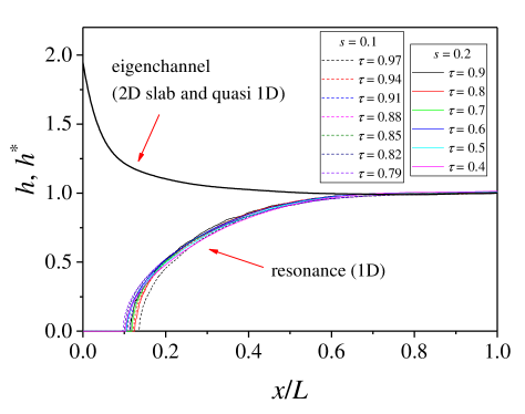
Figure 6: Simulations of the resonance structures in $1$D show that the $h^{*}$-function is universal with respect to both the resonant transmission $\mathcal{T}$ and the disorder strength $s$. This property is similar to the universality of the $h$-function that determines the eigenchannel structures in $2$D and quasi $1$D.

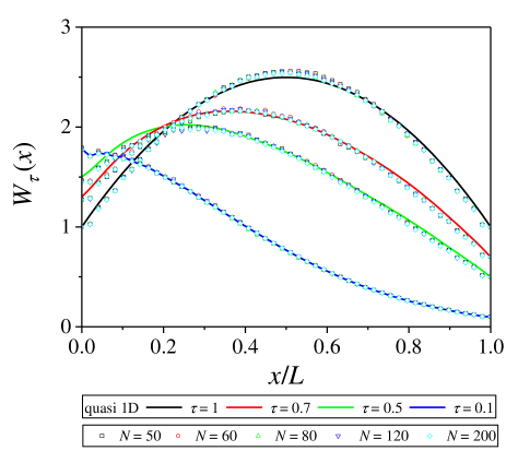
Figure 7: Simulations show that for $2$D slabs with different values of $N$, the ensemble averaged depth profile $W_{\tau}(x)$ (symbols) are well described by the analytic expression given by Eqs. (12)-(14) for quasi-$1$D waveguides (black solid lines). Note that at a given $\tau$ and $x$, all symbols for distinct $N$ overlap. $L$ is fixed to be $50$ and five ratios of $W/L$ are considered, which are $3$, $3.6$, $4.8$, $7.2$ and $12$, corresponding to $N=50$, $60$, $80$, $120$ and $200$, respectively.

III.2 Transverse structures of eigenchannels

We computed the Green’s function between grid points $(x^{\prime}=0,y^{\prime})$ and $(x,y^{\prime})$, where $0\leq x\leq L$. By using Eq. (3) we obtained the matrix $\bm{t}(x)$. Substituting the simulation results of $\{\bm{v}_{n}\}$ obtained before and $\bm{t}(x)$ into Eqs. (4) and (5) we found the profile $|\bm{E}_{\tau_{n}}(x,y)|^{2}$. We repeated the same procedures for many disorder configurations, and also for different widths.

Figure 1 represents an even more surprising phenomenon occurring for very large $W$ (corresponding to $N=800$ in simulations), regardless of the transmission eigenvalues. Basically, we see that the structure of $v_{n}(y)$ serves as a “skeleton” of the eigenchannel structure: each localization peak in $|v_{n}(y)|^{2}$ triggers a localization peak in the profile $|\bm{E}_{\tau_{n}}(x,y)|^{2}$ at arbitrary depth $x$. Thus at the cross section of arbitrary depth $x$, the transverse structure of eigenchannels is qualitatively the same as the localization structure of $|v_{n}(y)|^{2}$, i.e., if the latter has a single localization peak or exhibits a necklace structure, then so does the former, with the number of localization peaks being the same. Note that Fig. 1(b-d) correspond to the same disorder configuration and approximately the same transmission eigenvalue.

Furthermore, we introduce the $x$-dependent inverse participation ratio:

$$\frac{1}{\xi_{n}(x)}\equiv\left\langle\frac{\int dy|\bm{E}_{\tau_{n}}(x,y)|^{4}}{(\int dy|\bm{E}_{\tau_{n}}(x,y)|^{2})^{2}}\right\rangle$$ (9)

associated with the field distribution $\bm{E}_{\tau_{n}}(x,y)$ of the $n$th eigenchannel, where $\xi_{n}(x)$ characterizes the extension of the field distribution in the $y$ direction at the penetration depth $x$, and the average is over a number of $\bm{E}_{\tau_{n}}(x,y)$ corresponding to the same singular value $\tau_{n}$. Figure 3 presents typical numerical results of $\xi_{n}(x)$ for different values of $N$. From this it is easy to see that the field distribution has the same extension in the $y$ direction for every $x$, which is much smaller than $W$. This result provides a further evidence that the localization structure of $|v_{n}(y)|^{2}$ is maintained throughout the sample.

To understand the origin of the localization structures of eigenchannels, we first consider the case with single localization peak. We modify the input field $\bm{v}_{n}\equiv\{v_{n}(y)\}$ (panels a and b in Fig. 4) to be $\bm{v}^{\prime}_{n}\equiv\{v_{n}^{\prime}(y)\}$ (panel c) in the following way. We twist by $\pi$ the phase of $v_{n}(y)\equiv|v_{n}(y)|e^{i\varphi(y)}$ in certain region of $y$,

$$v_{n}(y)\rightarrow v^{\prime}_{n}(y)\equiv|v_{n}(y)|\exp\{i\varphi^{\prime}(y)\},$$ (10)

$$\varphi^{\prime}(y)=\varphi(y)+\pi\chi(y),$$ (11)

where $\chi(y)$ takes the value of unity in the region, and otherwise of zero. Then we let this modified input field propagate in the medium, $\bm{v}^{\prime}_{n}\rightarrow\bm{t}(x)\bm{v}^{\prime}_{n}$, and compare the ensuing $2$D energy density profile with the reference eigenchannel structure (panel d). We find that when the $\pi$-phase twist region is away from the localization center of $v_{n}(y)$ (panel c, dotted-dashed line), the resulting $2$D energy density profile is indistinguishable from the reference eigenchannel structure (panel e). That is, the eigenchannel structure is insensitive to modifications. Whereas for the changes made in the localization center (panel c, dashed line), the ensuing energy density profile is totally different from the reference eigenchannel structure (panel f). This shows that the localization structures of $|\bm{E}_{\tau_{n}}(x,y)|^{2}$ are of wave-coherence nature.

Next, we consider the case with two localization peaks. We modify the input field $\bm{v}_{n}\equiv\{v_{n}(y)\}$, which has two localization peaks [Fig. 5 (panel a)], in the same way as what was described by Eqs. (10) and (11), and let the modified input field propagate in the medium. We then compare the resulting $2$D energy density profile with the reference eigenchannel structure (panel b). Interestingly, if we perform the $\pi$-phase shift in one localization region of $|v_{n}(y)|^{2}$, then, for the ensuing $2$D energy density profile, only the peak adjacent to this localization peak of $|v_{n}(y)|^{2}$ is modified significantly, whereas the other is indistinguishable from the corresponding reference eigenchannel structure. This implies that when the transverse structure of eigenchannels if of the necklace-like shape, different localization peaks forming this necklace structure are incoherent. In addition, it provides a firm support that each localization peak in $|v_{n}(y)|^{2}$ triggers, independently, the formation of a single localization peak in the transverse structure of eigenchannels.

III.3 Universality of eigenchannel structures in slabs

Having analyzed the transverse structure of eigenchannels, we proceed to explore the longitudinal structure and to analyze its connection to the eigenchannel structure in a quasi $1$D diffusive waveguide.

For a quasi-$1$D diffusive waveguide the ensemble average of $w_{\tau}(x)$, denoted as $W_{\tau}(x)$, is given byTian15 :

$$W_{\tau}(x)=S_{\tau}(x)W_{\tau=1}(x),$$ (12)

where $W_{\tau=1}(x)$ is the profile corresponding to the transparent ($\tau=1$) eigenchannel,

$$W_{\tau=1}(x)=1+\frac{\pi Lx^{\prime}(1-x^{\prime})}{2\ell},\quad x^{\prime}=x/L,\quad$$ (13)

$$S_{\tau}(x)=2\frac{\cosh^{2}(h(x^{\prime})(1-x^{\prime})\phi)}{\cosh^{2}(h(x^{\prime})\phi)}-\tau,\quad\tau=\frac{1}{\cosh^{2}\phi},$$ (14)

with $\phi\geq 0$. Note that $h(x^{\prime})$ increases monotonically from $h(1)=1$ as $x^{\prime}$ decreases from $1$. Its explicit form, independent of $N,\tau$, is given in Fig. 6 (black solid curve).

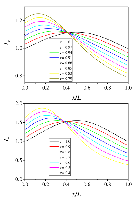
Figure 8: The ensemble-averaged resonance structure $I_{\mathcal{T}}(x)$ for two different disorder strengths: $s=0.1$ (top) and $s=0.3$ (bottom), whose corresponding localization-to-sample length ratios are $12$ and $3$, respectively.

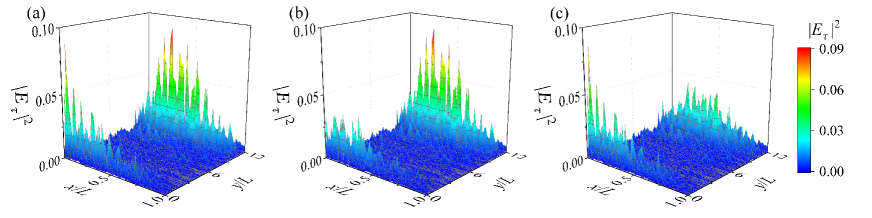
Figure 9: Simulations show that by shaping the input field $\bm{\psi}_{in}$, one can realize different profiles of energy density inside the medium. (a) The input field $\bm{\psi}_{in}=\frac{1}{\sqrt{2}}(\bm{v}_{h}+\bm{v}_{l})$, with $\bm{v}_{h(l)}$ corresponding to the right-singular vector of certain highly (low) transmitting eigenchannel. (b) The phase of $\bm{v}_{l}$ is twisted by $\pi$ in the region $0.3\leq y/L\leq 0.4$. (c) The phase of $\bm{v}_{h}$ is twisted by $\pi$ in the region $10.3\leq y/L\leq 10.4$.

Now we compare the eigenchannel structure in a slab with that in a quasi-$1$D waveguide described by Eqs. (12), (13) and (14). To this end we average $2000$ profiles of $w_{\tau}(x)$ with the same or close eigenvalues $\tau$. (Some of these eigenchannels may correspond to the same disorder configuration.) As a result, we obtain $W_{\tau}(x)$ for different values of $\tau$, shown in Fig. 7. We see, strikingly, that for slabs with different number of $N$ (i.e., width $W$) the structures of $W_{\tau}(x)$ are in excellent agreement with $W_{\tau}(x)$ described by Eqs. (12), (13) and (14).

IV Resonance structure

In the previous section, we have seen that in both $2$D slabs and quasi-$1$D waveguides the ensemble averaged eigenchannel structure $W_{\tau}(x)$ is described by the universal formula Eqs. (12), (13) and (14). It is natural to ask whether this universality can be extended to strictly $1$D systems, in which the transmission eigenchannel does not exist. Noting that the resonant transmissions have the same bimodal statistics as the transmission eigenvalues of eigenchannels Bliokh15 , in this section we study numerically the resonance structure ${\tilde{I}}_{\mathcal{T}_{n}}(x)$. It is well known Berezinskii73 that in strictly $1$D, there is no diffusive regime, because the localization length is $\sim\ell$. Instead, there are only ballistic and localized regimes. We consider the former below.

In simulations, the sample consists of $51$ scatterers separated by $50$ layers, whose thicknesses (rescaled by the inverse wave number in the background) are randomly distributed in the interval $d_{0}\pm\delta$, with $d_{0}=10.0$ and $\delta=9.0$. Thus $L=50d_{0}$. The scatterers are characterized by the reflection coefficients $r_{i}$ between the neighbouring layers ($i$ labels the scatterers.), which are chosen randomly and independently from the interval of $(-s,s)$, with $s\in(0,1)$ governing the disorder strength. We change the frequency $\Omega$ in a narrow band centered at $\Omega_{0}$ and of half-width $5\%\times\Omega_{0}$, and calculate the transmittance spectrum $\mathcal{T}(\Omega)$ by using the standard transfer matrix approach. We also change disorder configurations, so that for each resonant transmission $\mathcal{T}_{n}$, $5\times 10^{5}$ profiles of ${\tilde{I}}_{\mathcal{T}_{n}}(x)$ are obtained. We then calculate the average of these profiles, denoted by $I_{\tau_{n}}(x)$. Finally, we repeat the numerical experiments for different values of $s$.

Figure 8 shows the simulation results of $I_{\tau}(x)$ for two different values of $s$. These profiles look similar to those presented in Fig. 7. For quantitative comparison, we compute the quantity $S_{\tau}^{*}(x)\equiv I_{\tau}(x)/I_{\tau=1}(x)$. Then, we present the function $S_{\tau}^{*}(x)$ in the form:

$$S_{\tau}^{*}(x)=2\frac{\cosh^{2}(h^{*}(x^{\prime})(1-x^{\prime})\phi)}{\cosh^{2}(h^{*}(x^{\prime})\phi)}-\tau,$$ (15)

and find $h^{*}(x^{\prime})$ for different values of $\tau$ and $s$ from $S_{\tau}^{*}(x)$ calculated numerically (Fig. 6). The results are surprising: as shown in Fig. 6, $h^{*}(x^{\prime})$ is a universal function, independent of $\tau$ and $s$, which is the key feature of $h(x^{\prime})$ for eigenchannel structures. However, Fig. 6 also shows that the two universal functions, i.e., $h^{*}(x^{\prime})$ and $h(x^{\prime})$, are different. Therefore, allowing this minimal modification, the expression described by Eqs. (12), (13) and (14) is super-universal: it applies to both the resonance structure and the eigenchannel structure.

V Possible applications

The universal properties of the transmission eigenchannels presented above open up outstanding possibilities to tailor the energy distribution inside higher-dimensional opaque materials, in particular, to concentrate energy in different parts of a diffusive sample. In the example shown in Fig. 9, two eigenchannels with low ($\tau_{l}=0.1$) and high ($\tau_{h}=1$) transmissions were exited, so that the input field had the form $\bm{\psi}_{in}=\frac{1}{\sqrt{2}}(\bm{v}_{h}+\bm{v}_{l})$. Here the right-singular vector $\bm{v}_{h(l)}\equiv\{v_{h(l)}(y)\}$ of the TM corresponds to a highly (low) transmitting eigenchannel. It is easy to see that the energy density profile generated by this input inside the medium is comprised of two phase coherent, but spatially separated parts. This is because the initial transverse localization of $\bm{v}_{h(l)}$ holds along the sample, and the integrated energy density profiles given by Eqs. (12), (13) and (14) have maxima at different points $x$ (i.e., the higher is the transmission eigenvalue, the larger is the radiation penetration depth).

Simulations further show (Fig. 9) that it is possible, without changing the topology of the profile, to vary the relative intensity deposited in the two separated regions by simply modulating the phase field of $\bm{\psi}_{in}$. For example, if we twist the phase $\varphi_{l}(y)$ of $v_{l}(y)$ at points $y$ near the localization center [of $v_{l}(y)$] by $\pi$,

$$v_{l}(y)\rightarrow v^{\prime}_{l}(y)=|v_{l}(y)|\exp\{i\varphi^{\prime}_{l}(y)\},$$ (16)

$$\varphi^{\prime}_{l}(y)=\varphi_{l}(y)+\pi\chi(y),$$ (17)

where $\chi(y)$ takes the value of unity in a region near the localization center and otherwise is zero. For the ensuing input field $\bm{\psi}_{in}=\frac{1}{\sqrt{2}}(\bm{v}_{h}+\bm{v}^{\prime}_{l})$, where $\bm{v}^{\prime}_{l}\equiv\{v^{\prime}_{l}(y)\}$, we find that the energy density deposited in the region corresponding to the low transmission eigenchannel is suppressed. Similarly, we can modify the input field to suppress the energy density deposited in the region corresponding to the high transmission eigenchannel.

VI Conclusions and outlook

Summarizing, we have shown that in a diffusive medium, as the medium geometry crosses over from quasi-$1$D to higher dimension, despite the transverse structure of eigenchannels (corresponding to the same transmission eigenvalues) undergo dramatic changes, i.e., from the extended to the Anderson-like localized or necklace-like distributions, their longitudinal structure stays the same, i.e., the depth profile $W_{\tau}(x)$ of the energy density of an eigenchannel with transmission $\tau$ is always described by Eqs. (12)-(14), regardless of medium geometry. The details of the system, such as the thickness and the disorder ensemble, only enter into the ratio of $L/\ell$ in Eq. (12). This expression is super-universal, i.e., it encompasses not only the energy distributions in diffusive eigenchannels in any dimension, but (with a minimal modification) the shape of the transmission resonances in strictly 1D random systems as well. These findings suggest that eigenchannels, which are the underpinnings of diverse diffusive wave phenomena in any dimension, might have a common origin, namely, $1$D resonances. Although the similarity between the eigenchannel structure and the Fabry-Perot cavity has been noticed already in the pioneer study of eigenchannel structures Choi11 , a comprehensive study of this phenomenon has not been carried out. The results presented above may already be helpful in further advancing the methods of focusing coherent light through scattering media by wavefront shaping. Another area of potential applications is random lasing Cao99 ; Wiersma08 in diffusive media. Moreover, based on previous studies Tian13 ; Bliokh15 ; Lagendijk16a ; Tian17 , we expect that controlling the reflectivities of the edges of a sample one can tune the intensity distributions in eigenchannels, not only in quasi-1D media, but in samples of higher dimensions as well. In the future, it is desirable to explore the super-universality of eigenchannel structures in high-dimensional media, where wave interference is strong, so that Anderson localization or an Anderson localization transition occurs.

References

- (1) S. Rotter and S. Gigan, Rev. Mod. Phys. 89, 015005 (2017).
- (2) I. M. Vellekoop and A. P. Mosk, Phys. Rev. Lett. 101, 120601 (2008).
- (3) W. Choi, A. P. Mosk, Q. H. Park, and W. Choi, Phys. Rev. B 83, 134207 (2011).
- (4) M. Kim, Y. Choi, C. Yoon, W. Choi, J. Kim, Q-H. Park, and W. Choi, Nat. Photon. 6, 581 (2012).
- (5) A. P. Mosk, A. Lagendijk, G. Lerosey, and M. Fink, Nat. Photon. 6, 283 (2012).
- (6) M. Davy, Z. Shi, and A. Z. Genack, Phys. Rev. B 85, 035105 (2012).
- (7) M. Davy, Z. Shi, J. Park, C. Tian, and A. Z. Genack, Nat. Commun. 6, 6893 (2015).
- (8) S. F. Liew and H. Cao, Opt. Express 23, 11043 (2015).
- (9) O. S. Ojambati, A. P. Mosk, I. M. Vellekoop, A. Lagendijk, and W. L. Vos, Opt. Express 24, 18525 (2016).
- (10) R. Sarma, A. G. Yamilov, S. Petrenko, Y. Bromberg, and H. Cao, Phys. Rev. Lett. 117, 086803 (2016).
- (11) M. Koirala, R. Sarma, H. Cao, and A. Yamilov, Phys. Rev. B 96, 054209 (2017).
- (12) C. W. Hsu, S. F. Liew, A. Goetschy, H. Cao, and A. D. Stone, Nat. Phys. 13, 497 (2017).
- (13) O. S. Ojambati, H. Yilmaz, A. Lagendijk, A. P. Mosk, and W. L. Vos, New J. Phys. 18, 043032 (2016).
- (14) P. L. Hong, O. S. Ojambati, A. Lagendijk, A. P. Mosk, and W. L. Vos, Optica 5, 844 (2018).
- (15) H. Yilmaz, C. W. Hsu, A. Yamilov, and H. Cao, arXiv: 1806.01917.
- (16) see Section S2 in Supplemental Materials of: P. Fang, L. Y. Zhao, and C. Tian, Phys. Rev. Lett. 121, 140603 (2018).
- (17) O. N. Dorokhov, Pis’ma Zh. Eksp. Teor. Fiz. 36, 259 (1982); [JETP Lett. 36, 318 (1982)].
- (18) O. N. Dorokhov, Solid State Commun. 51, 381 (1984).
- (19) P. A. Mello, P. Pereyra, and N. Kumar, Ann. Phys. (N.Y.) 181, 290 (1988).
- (20) C. W. J. Beenakker, Rev. Mod. Phys. 69, 731 (1997).
- (21) L. Y. Zhao, C. Tian, Y. P. Bliokh, and V. Freilikher, Phys. Rev. B 92, 094203 (2015).
- (22) K. Y. Bliokh, Y. P. Bliokh, and V. D. Freilikher, J. Opt. Soc. Am. B 21, 113 (2004).
- (23) P. W. Anderson, Phys. Rev. 109, 1492 (1958).
- (24) M. E. Gertsenshtein and V. B. Vasil’ev, Teor. Veroyatn. Primen. 4, 424 (1959) [Theor. Probab. Appl. 4, 391 (1959)].
- (25) K. Yu. Bliokh, Yu. P. Bliokh, V. Freilikher, S. Savel’ev, and F. Nori, Rev. Mod. Phys. 80, 1201 (2008).
- (26) H. U. Baranger, D. P. DiVincenzo, R. A. Jalabert, and A. D. Stone, Phys. Rev. B 44, 10637 (1991).
- (27) A. MacKinnon, Z. Phys. B 59, 385 (1985).
- (28) G. Metalidis and P. Bruno, Phys. Rev. B 72, 235304 (2005).
- (29) Yu. V. Nazarov, Phys. Rev. Lett. 73, 134 (1994).
- (30) V. L. Berezinskii, Zh. Eksp. Teor. Fiz. 65, 1251 (1973) [Sov. Phys. JETP 38, 620 (1974)].
- (31) H. Cao, Y. G. Zhao, S. T. Ho, E. W. Seelig, Q. H. Wang, and R. P. H. Chang, Phys. Rev. Lett. 82, 2278 (1999).
- (32) D. S. Wiersma, Nature Phys. 4, 359 (2008).
- (33) X. J. Cheng, C. S. Tian, and A. Z. Genack, Phys. Rev. B 88, 094202 (2013).
- (34) D. Akbulut, T. Strudley, J. Bertolotti, E. P. A. M. Bakkers, A. Lagendijk, O. L. Muskens, W. L. Vos, and A. P. Mosk, Phys. Rev. A 94, 043817 (2016).
- (35) X. Cheng, C. Tian, Z. Lowell, L. Y. Zhao, and A. Z. Genack, Eur. Phys. J. Special Topics 226, 1539 (2017).