Impact of the neutron star crust on the tidal polarizability

Abstract

Background: The first direct detection of a binary neutron star merger (GW170817) by the LIGO-Virgo scientific collaboration has opened the brand new era of multimessenger astronomy. This historic detection has been instrumental in providing initial constraints on the tidal polarizability (or deformability) of neutron stars. In turn, the tidal polarizability—an observable highly sensitive to stellar compactness—has been used to impose limits on stellar radii and ultimately on the underlying equation of state (EOS). Purpose: Besides its strong dependence on the stellar compactness, the tidal polarizability is also sensitive to the second tidal Love number $k_{2}$. It is the main purpose of this work to perform a detailed study of $k_{2}$ which, for a given compactness parameter, encodes the entire sensitivity of the tidal polarizability to the underlying equation of state. In particular, we examine the important role that the crustal component of the EOS plays in the determination of $k_{2}$. Methods: A set of realistic models of the equation of state that yield an accurate description of the properties of finite nuclei, support neutron stars of two solar masses, and provide a Lorentz covariant extrapolation to dense matter are used to solve both the Tolman-Oppenheimer-Volkoff and the differential equation for the induced quadrupole gravitational field from which $k_{2}$ is extracted. Results: Given that the tidal polarizability scales as the fifth power of the compactness parameter, a universal relation exists among the tidal polarizability and the compactness parameter that is highly insensitive to the underlying equation of state. Thus, besides an extraction of the tidal polarizabilities, a measurement of the individual stellar masses is also required to impact the mass-radius relation. However, we observe a strong sensitivity of the second Love number to the underlying equation of state—particularly to the contribution from the inner crust. Conclusions: Although by itself the tidal polarizability can not contribute to the determination of the mass-radius relation, future detections of binary neutron star mergers by the LIGO-Virgo collaboration during the third observing run and beyond are poised to provide significant constraints on both the tidal polarizabilities and masses of the individual stars, and thus ultimately on the mass-radius relation. Yet, subleading corrections to the tidal polarizability are encoded in the second Love number $k_{2}$ which displays a large sensitivity to the entire—crust-plus-core—equation of state.

I Introduction

Nuclear physics plays a predominant role in explaining the behavior of neutron stars. Neutron stars are fascinating objects that are born from the collapse of massive stars and reach central densities that may exceed those found in atomic nuclei by up to an order of magnitude. In contrast to the common perception of neutron stars as “dense stars which look like one giant nucleus” Landau (1932); Yakovlev et al. (2013), their structure, dynamics, and composition are much richer and far more interesting. Structurally, neutron stars contain both a solid crust and a liquid core. The non-uniform crust sits above a uniform liquid core that largely conforms to the perception of a neutron star as a giant assembly of closed packed neutrons, protons, and leptons. Note that protons and leptons are fundamental stellar constituents that are required to maintain chemical equilibrium and enforce charge neutrality. However, the non-uniform crust deviates drastically from such a naive picture, as it is populated by fascinating and novel states of matter. Yet, the one kilometer stellar crust plays a rather modest role in the structure of the star. Indeed, the liquid core accounts for practically all the mass and about 90% of the size of a neutron star. Yet, we suggest here that the second tidal Love number Binnington and Poisson (2009); Damour et al. (2012), a quantity of great relevance to the tidal polarizability (or deformability) of neutron stars, is sensitive to the poorly known crustal equation of state. Our study is motivated by the first direct detection of the binary neutron star merger GW170817 Abbott et al. (2017) that is providing fundamental new insights into the nature of dense matter, primarily through constraints on the tidal polarizability. Although GW170817 has been instrumental in elucidating the site of the $r$-process and confirming the association between binary neutron star mergers and short-gamma ray bursts, much activity has also been devoted to explore the impact of GW170817 on the equation of state (EOS). In particular, constraints on the tidal polarizability from the gravitational wave profile have already been used to impose limits on stellar radii and ultimately on the EOS Bauswein et al. (2017); Fattoyev et al. (2018); Annala et al. (2018); Abbott et al. (2018); Most et al. (2018); Tews et al. (2018); Malik et al. (2018); Tsang et al. (2018); Radice and Dai (2018).

To place our work in the proper context, we now present a brief description of the main features of the stellar crust. At the typical densities of the outer crust, ranging from about $10^{4}{\rm g/cm^{3}}$ to $4\!\times\!10^{11}{\rm g/cm^{3}}$ Baym et al. (1971), the electrons have been pressure ionized and move freely as a relativistic free Fermi gas. However, as compared with the typical densities found at the center of atomic nuclei, of the order of nuclear matter at saturation $\rho_{\raisebox{-0.75pt}{\tiny 0}}\!=\!0.15\,{\rm fm}^{-3}\!\simeq\!2.5\!\times\!10^{14}{\rm g/cm^{3}}$, these crustal densities are considerably smaller, resulting in an average inter-nucleon separation much larger than the range of the nucleon-nucleon interaction. Thus, it becomes energetically favorable for nucleons to cluster into finite nuclei which arrange themselves in a crystalline lattice. Having the lowest mass per nucleon in the entire nuclear chart, ⁵⁶Fe is the most favorable nucleus at the lowest densities found in the outer crust. However, as the density increases and with it the electronic contribution to the energy, ⁵⁶Fe ceases to be the nucleus of choice. Indeed, it becomes energetically advantageous for electrons to capture onto protons and for the excess energy to be carried away by neutrinos. As such, the system evolves into a Coulomb crystal of progressively more exotic neutron-rich nuclei, ranging from ⁶²Ni up to (likely) ¹¹⁸Kr—a “drip nucleus” with 32 more neutrons than its heaviest stable isotope ⁸⁶Kr Roca-Maza and Piekarewicz (2008). The equation of state of the outer crust is fairly simple to understand as it is dominated by the electronic contribution with a small correction from the crystalline lattice. The major uncertainty in the EOS emerges from the absence of experimentally determined masses for the most exotic nuclei populating the crystal lattice which, in turn, set the electron fraction in the crust.

Below the outer crust sits the inner crust spanning a region from the neutron-drip density of $4\!\times\!10^{11}{\rm g/cm^{3}}$ up to the transition density to the uniform liquid core. At the top layers of the inner crust nucleons continue to cluster into a Coulomb crystal of neutron-rich nuclei embedded in a uniform electron gas. Now, however, the crystal is also in equilibrium with a dilute, likely superfluid, neutron vapor. As the density increases, the spherical nuclei that form the crystal lattice start to deform in an effort to reduce the Coulomb repulsion, resulting in the formation of rich and complex structures collectively referred to as nuclear pasta Ravenhall et al. (1983); Hashimoto et al. (1984). Moreover, due to the preponderance of quasi-degenerate low-energy states—a hallmark of “Coulomb frustration”—these systems display an interesting yet subtle low-energy dynamics that has been captured using either semi-classical simulations Horowitz et al. (2004a, b); Horowitz et al. (2005); Watanabe et al. (2003, 2005, 2009); Schneider et al. (2013); Horowitz et al. (2015); Caplan et al. (2015) or quantum-mechanical mean-field approaches Bulgac and Magierski (2001); Magierski and Heenen (2002); Chamel (2005); Newton and Stone (2009); Schuetrumpf and Nazarewicz (2015); Fattoyev et al. (2017). Yet despite the undeniable progress in understanding the nuclear-pasta phase, we are unaware of any theoretical framework that simultaneously incorporates quantum-mechanical effects and dynamical correlations beyond the mean-field level. As a result, a reliable equation of state for the inner crust is still missing. In the past, we have adopted a simple polytropic interpolation formula Link et al. (1999) to estimate the equation of state in the inner crust Carriere et al. (2003). The central goal of this work is to examine the sensitivity of the tidal Love number to the unknown EOS in the inner stellar crust.

We have organized the paper as follows. In Sec. II we review the essential details required to compute the tidal polarizability and its expected sensitivity to the choice of equation of state. In particular, special attention is paid to the component of the equation of state used to model the inner crust. In Sec. III we provide predictions for the second Love number and examine its sensitivity to the various choices for the equation of state. In particular, we show that although the crustal component of the EOS plays a minor role in the determination of both the radius and the mass, it has a significant impact on the Love number. Finally, we summarize and conclude in Sec. IV.

II Formalism

The formalism is divided into two main components, one dedicated to the description of the underlying equation of state and the other one to the calculation of the second tidal Love number from which the tidal polarizability can be readily computed.

II.1 Equation of State

II.1.1 Liquid Core

Our starting point is a particular class of relativistic effective field theories containing as elementary constituents an isodoublet nucleon field ($\psi$) interacting via the exchange of two isoscalar mesons—the scalar sigma ($\phi$) and the vector omega ($V^{\mu}$)—one isovector meson, the rho (${\bf b}^{\mu}$), and the photon ($A^{\mu}$). Besides conventional Yukawa couplings Walecka (1974), the model is supplemented by nonlinear self Boguta and Bodmer (1977); Serot and Walecka (1986); Mueller and Serot (1996) and mixed Horowitz and Piekarewicz (2001a); Todd-Rutel and Piekarewicz (2005); Chen and Piekarewicz (2014) interactions between the mesons that are critical to improve the quantitative standing of the model. The interacting Lagrangian density describing such class of effective theories is given by Chen and Piekarewicz (2014):

$${\mathscr{L}}_{\rm int} = \bar{\psi}\left[g_{\rm s}\phi\!-\!\left(g_{\rm v}V_{\mu}\!+\!\frac{g_{\rho}}{2}{\mbox{\boldmath$\tau$}}\cdot{\bf b}_{\mu}\!+\!\frac{e}{2}(1\!+\!\tau_{3})A_{\mu}\right)\gamma^{\mu}\right]\psi$$ (1)

$$- \frac{\kappa}{3!}(g_{\rm s}\phi)^{3}\!-\!\frac{\lambda}{4!}(g_{\rm s}\phi)^{4}\!+\!\frac{\zeta}{4!}g_{\rm v}^{4}(V_{\mu}V^{\mu})^{2}+\Lambda_{\rm v}\Big{(}g_{\rho}^{2}\,{\bf b}_{\mu}\cdot{\bf b}^{\mu}\Big{)}\Big{(}g_{\rm v}^{2}V_{\nu}V^{\nu}\Big{)}\;.$$

The non-linear scalar couplings ($\kappa$ and $\lambda$) pioneered by Boguta and Bodmer are responsible for softening the equation of state of symmetric nuclear matter near saturation density Boguta and Bodmer (1977). This softening reduces the compressibility coefficient of symmetric nuclear matter and is instrumental in bringing theoretical calculations of the isoscalar monopole response into agreement with experiment. The omega-meson self-coupling $\zeta$ also softens the equation of state of symmetric nuclear matter, but at much higher densities. By tuning this single parameter, one can generate neutron stars with maximum masses that vary by more than one solar mass while retaining agreement with laboratory observables Mueller and Serot (1996). Finally, the nonlinear mixed coupling $\Lambda_{\rm v}$ is highly sensitive to the density dependence of symmetry energy and in particular to its slope at saturation density—a quantity with a strong impact on the structure and dynamics of both exotic neutron-rich nuclei and neutron stars Horowitz and Piekarewicz (2001a, b); Carriere et al. (2003); Horowitz et al. (2004a); Chen and Piekarewicz (2014, 2015).

In the spirit of density functional theory, the parameters of the model are directly fitted to laboratory observables, such as binding energies and charge radii of magic and semi-magic nuclei. Whereas most of the parameters are well calibrated by such fitting protocol, two of them—$\Lambda_{\rm v}$ and $\zeta$—are sensitive to physics that has not yet been efficiently probed in either laboratory experiments or astrophysical observations. This lack of sensitivity could be remedied by probing isovector observables with a large neutron excess, such as the thickness of the neutron skin of neutron-rich nuclei, or observables sensitive to the high density behavior of the EOS, such as the maximum neutron-star mass Fattoyev and Piekarewicz (2011, 2012); Chen and Piekarewicz (2014). One could also constrain these poorly determined parameters by exploring their impact on novel neutron-star observables, such as the tidal polarizability. Yet, it is important to underscore that the above model is used exclusively to compute the equation of state of the uniform liquid core; that is, the phase consisting of a uniform, charged-neutral system composed of neutrons, protons, electrons, and muons in chemical equilibrium.

The equation of state of cold neutron-rich matter describes the connection between the energy density, the pressure, and the baryon density of the system. At zero temperature, the energy density and pressure (both intensive quantities) are functions exclusively of the conserved baryon density $\rho\!=\rho_{n}\!+\!\rho_{p}$ and the neutron-proton asymmetry $\alpha\!\equiv\!(\rho_{n}\!-\!\rho_{p})/(\rho_{n}\!+\!\rho_{p})$. To identify a few of the critical properties of the EOS it is customary to expand the energy per nucleon in even powers of $\alpha$:

$$\frac{E}{A}(\rho,\alpha)-\!M\equiv{\cal E}(\rho,\alpha)={\cal E}_{\rm SNM}(\rho)+\alpha^{2}{\cal S}(\rho)+{\cal O}(\alpha^{4})\,,$$ (2)

where ${\cal E}_{\rm SNM}(\rho)\!=\!{\cal E}(\rho,\alpha\!\equiv\!0)$ is the energy per nucleon of symmetric nuclear matter (SNM) and the symmetry energy ${\cal S}(\rho)$ represents to a good approximation the energy cost of converting symmetric nuclear matter into pure neutron matter. Also customary is to encode the behavior of both symmetric nuclear matter and the symmetry energy in the vicinity of saturation density $\rho_{\raisebox{-0.75pt}{\tiny 0}}$ in terms of a few bulk parameters. Introducing $x\!=\!(\rho\!-\!\rho_{\raisebox{-0.75pt}{\tiny 0}})\!/3\rho_{\raisebox{-0.75pt}{\tiny 0}}$ to quantify the deviations of the EOS from its value at saturation density we obtain Piekarewicz and Centelles (2009),

$${\cal E}_{\rm SNM}(\rho)=\varepsilon_{\raisebox{-0.75pt}{\tiny 0}}+\frac{1}{2}Kx^{2}+\ldots,$$ (3a)

$${\cal S}(\rho)=J+Lx+\frac{1}{2}K_{\rm sym}x^{2}+\ldots$$ (3b)

Given that the saturation of symmetric nuclear matter is one of the hallmarks of the nuclear dynamics, accurately-calibrated models that are informed by the binding energy and charge radius of a variety of nuclei predict the saturation point at a density of $\rho_{\raisebox{-0.75pt}{\tiny 0}}\simeq\!0.15\,{\rm fm}^{-3}$ and an energy per particle of $\varepsilon_{\raisebox{-0.75pt}{\tiny 0}}\!\simeq\!-16\,{\rm MeV}$. As a result, the pressure of symmetric nuclear matter vanishes at saturation, so the small density fluctuations around the saturation point are controlled by the incompressibility coefficient $K$.

However, unlike symmetric nuclear matter, pure neutron matter does not saturate. As a result, the pressure of pure neutron matter at saturation ($P_{0}$) does not vanish. This suggests that the behavior of the symmetry energy around saturation density is largely contained in three, rather than two, bulk parameters: its value $J$, its slope $L$, and its curvature $K_{\rm sym}$ at saturation density. Note that in the so-called parabolic approximation Piekarewicz and Centelles (2009) the slope of the symmetry energy $L$ is directly proportional to the pressure of pure neutron matter. That is,

$$P_{0}=\frac{1}{3}\rho_{\raisebox{-0.75pt}{\tiny 0}}L\;.$$ (4)

The Lagrangian density introduced in Eq. (1) will be used to compute both the equation of state of the uniform liquid core as well as properties associated with the transition from the liquid core to the solid crust. The development of a non-uniform crust is largely due to the short-range nature of the strong interaction. At densities at which the inter-nucleon separation in the uniform system becomes larger than the range of the nucleon-nucleon interaction, it becomes energetically advantageous for nucleons to cluster into finite nuclei in order to benefit from the nuclear attraction. To describe the crust-to-core transition one determines the density at which the uniform liquid becomes unstable against small amplitude density oscillations. The instability may be determined dynamically by implementing the relativistic random-phase-approximation (RPA) described in Ref. Carriere et al. (2003). The outcome of such RPA analysis is the transition density together with the associated pressure and energy density at which the instability develops. In particular, the transition density is strongly sensitive to the density dependence of the symmetry energy, particularly to its slope at saturation density $L$ Horowitz and Piekarewicz (2001a).

II.1.2 Outer Crust

Before discussing the equation of state in the inner crust we address the simpler dynamics of the outer crust—the low-density region in which all neutrons are bound to finite nuclei. The dynamics of the outer crust is encapsulated in a relatively simple expression for the total Gibbs free energy per nucleon, which at zero temperature equals the total chemical potential of the system. That is Haensel et al. (1989); Haensel and Pichon (1994); Ruester et al. (2006); Roca-Maza and Piekarewicz (2008); Roca-Maza et al. (2011),

$$\mu(Z,A;P)=\frac{M(Z,A)}{A}+\frac{Z}{A}\mu_{e}-\frac{4}{3}C_{l}\frac{Z^{2}}{A^{4/3}}\,p_{{}_{\rm F}},$$ (5)

where $Z$ and $A$ are the atomic and mass number of the “optimal” finite nucleus (to be defined shortly) and P is the pressure of the system, which is dominated by the degenerate electrons. To use the above equation it is necessary to provide a connection between the pressure and the baryon density of the system $\rho$, or its proxy the Fermi momentum $p_{{}_{\rm F}}$ that is defined as follows:

$$p_{{}_{\rm F}}=\left(3\pi^{2}\rho\right)^{1/3}.$$ (6)

The connection between the pressure and the baryon density is encoded in the equation of state of a body-centered-cubic lattice of neutron-rich nuclei embedded in a uniform electron gas. That is Baym et al. (1971); Roca-Maza and Piekarewicz (2008),

$$P(\rho)=\frac{m_{e}^{4}}{3\pi^{2}}\left(x_{{}_{\rm F}}^{3}y_{{}_{\rm F}}\!-\!\frac{3}{8}\left[x_{{}_{\rm F}}y_{{}_{\rm F}}\Big{(}x_{{}_{\rm F}}^{2}\!+\!y_{{}_{\rm F}}^{2}\Big{)}\!-\!\ln(x_{{}_{\rm F}}\!+\!y_{{}_{\rm F}})\right]\right)\!-\!\frac{\rho}{3}C_{l}\frac{Z^{2}}{A^{4/3}}\,p_{{}_{\rm F}}.$$ (7)

Here $x_{{}_{\rm F}}\!=\!p_{{}_{\rm F}}^{e}/m_{e}$ and $y_{{}_{\rm F}}\!=\!(1\!+\!x_{{}_{\rm F}}^{2})^{1/2}$ are scaled electronic Fermi momentum and Fermi energy expressed in terms of the electronic Fermi momentum $p_{{}_{\rm F}}^{e}\!=\!(Z/A)^{1/3}p_{{}_{\rm F}}$ and $C_{l}\!=\!3.40665\!\times\!10^{-3}$ is the dimensionless lattice constant Roca-Maza and Piekarewicz (2008). The first term in Eq. (5) is independent of the pressure and represents the entire nuclear contribution to the chemical potential. It depends exclusively on the mass per nucleon of the optimal nucleus populating the lattice. The second term represents the contribution from a relativistic free Fermi gas of electrons. As such, it is strongly density dependent and represents the major contribution to the pressure. Finally, the last “screening” term provides the relatively modest lattice contribution to the pressure.

The above discussion suggests that the only unknown in the determination of the crustal composition is the optimal nucleus $(Z,A)_{\rm opt}$ populating the crystal lattice. To determine the optimal nucleus we implement the following procedure for each value of the pressure $P$ and for every chosen nuclear mass model, which often consists of thousands of nuclei. Given an individual nucleus $(Z,A)$ in the mass table, one computes the chemical potential $\mu(Z,A;P)$, which requires the determination of the baryon density by inverting Eq. (7). The optimal nucleus is defined as the one that minimizes the overall chemical potential. For low densities, the electronic contribution is modest so the optimal nucleus is found to be ⁵⁶Fe, the nucleus with the lowest mass per nucleon in the entire nuclear chart. As the electronic contribution increases, it becomes energetically favorable for electrons to capture into protons, thereby reducing the electron fraction albeit at the expense of increasing the neutron-proton asymmetry. Ultimately, the crustal composition emerges from a subtle competition between the electronic contribution that favors $Z/A\!=\!0$, and the nuclear symmetry energy which favors nearly symmetric nuclei. This procedure continues until the chemical potential becomes equal to the mass of the neutron. Beyond this pressure the drip line is reached as the optimal nucleus is unable to hold any more neutrons. This defines the transition region from the outer crust to the inner crust. Note that the composition of the outer crust determined in this manner requires knowledge of the masses of a few exotic nuclei that are presently beyond experimental reach. To determine such masses one must rely on uncontrolled theoretical extrapolations. To mitigate this problem machine learning is becoming an important tool to estimate, with proper theoretical errors, the unknown masses of a variety of exotic nuclei Bayram et al. (2014); Utama et al. (2016); Utama and Piekarewicz (2017, 2018); Neufcourt et al. (2018). Note that most of these nuclei are unstable under normal laboratory conditions, yet become stable in the outer crust because of the presence of the neutralizing electron background.

II.1.3 Inner Crust

Based on the previous discussion, two well determined boundaries are relevant to the calculation of the structural properties of a neutron star: (a) the transition from the outer to the inner crust defined as the region in which the chemical potential equals the neutron mass and (b) the transition from the inner crust to the liquid core identified as the density at which the uniform ground state become unstable to density fluctuations. How then does one connect these two regions? The answer to this question is highly complex. Length scales that were well separated in both the crystalline phase, where the long-range Coulomb interaction dominates, and in the uniform phase, where the short-range nuclear interaction prevails, are now comparable. This gives rise to a universal phenomenon known as Coulomb frustration. At densities of relevance to the inner crust, Coulomb frustration drives the formation of the nuclear-pasta phase, characterized by the emergence of complex topological structures dubbed “nuclear pasta” Ravenhall et al. (1983); Hashimoto et al. (1984); for some recent reviews on the captivating structure and dynamics of the neutron-star crust see Refs. Chamel and Haensel (2008); Bertulani and Piekarewicz (2012) and references contained therein.

Although dynamically fascinating, the precise role of the nuclear pasta in the determination of the equation of state is still unknown. In the past, we have followed the suggestion given in Ref. Link et al. (1999) and adopted a simple polytropic interpolation between the outer crust and the liquid core Carriere et al. (2003). That is,

$$P({{\varepsilon}})=A+B{{\varepsilon}}^{\,4/3},$$ (8)

where ${{\varepsilon}}$ is the energy density of the system, and the two constants $A$ and $B$ are chosen so that the pressure is continuous at both (a) the boundary between the inner and the outer crusts and (b) the boundary between the inner crust and the liquid core. However, unlike the Tolman-Oppenheimer-Volkoff equations that depend exclusively on the equation of state $P\!=\!P({{\varepsilon}})$, the corresponding differential equation required to compute the tidal polarizability is also sensitive to its derivative, i.e., to the speed of sound; see Sec. II.2. Hence, as a simple test of the sensitivity of the tidal polarizability to the choice of EOS in the inner crust, we adopt a cubic interpolation formula so that both the pressure and its first derivative are continuous at both interphases. Note, however, that every change in the composition of the outer crust is accompanied by a discontinuity in the speed of sound Han and Steiner (2018).

In summary, the following prescription has been adopted for the equation of state. First, the equation of state for the outer crust is defined at minimum values of $P_{\rm min}\!=\!6.08\times 10^{-15}$ MeV/fm³ and ${{\varepsilon}}_{\rm min}\!=\!5.86\times 10^{-9}$ MeV/fm³ for the pressure and energy density, respectively, as prescribed in the seminal work of Baym, Pethick, and Sutherland (BPS) Baym et al. (1971). The corresponding maximum values for the pressure and energy density are determined by demanding that the chemical potential introduced in Eq.(5) be equal to the bare neutron mass. Note, however, that we modify slightly the BPS equation of state by using the improved Duflo-Zuker mass formula Duflo and Zuker (1995) to compute the composition of the outer crust. Second, given the complexity of the inner crust, we adopted an equation of state that interpolates between the corresponding EOSs in the outer crust and in the liquid core, with the inner crust-core boundary determined from the RPA analysis outlined above. Finally, beyond this transition region, the equation of state in the uniform liquid core is derived from the Lagrangian density given in Eq.(1). As an example, the equation of state predicted by the relativistic density functional “FSUGarnet” Chen and Piekarewicz (2015) is shown in Fig.1. Although imperceptible in the log-log scale used in the figure, the EOS in the outer crust displays various “jumps” that are associated with changes in the nuclear composition.

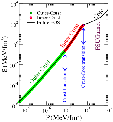
Figure 1: (Color online) Neutron-star-matter equation of state as predicted by the relativistic density functional “FSUGarnet” Chen and Piekarewicz (2015). The features that are sensitive to the choice of density functional are the crust-core transition pressure and the EOS in the entire uniform liquid core.

II.2 Tidal Polarizability

As alluded in the Introduction, the first direct detection of gravitational waves from the binary neutron star merger GW170817 Abbott et al. (2017) is providing fundamental new insights into the nature of dense matter. Critical properties of the equation of state are encoded in the tidal polarizability of the neutron star, an intrinsic property that describes its tendency to develop a mass quadrupole in response to the tidal field induced by its companion Damour et al. (1992); Flanagan and Hinderer (2008). As the two neutron stars approach each other and tidal effects become important, the phase of the gravitational wave is modified from its point-mass nature characteristic of black holes. How “early” during the inspiral phase do tidal effects become important is highly sensitive to the compactness of the star, and ultimately to the underlying equation of state. For a given mass, a star with a large radius is “fluffy” and therefore more sensitive to tidal effects. Such a star would deform earlier in the inspiral than the correspondingly smaller (more compact) star. One of the main findings of the LIGO-Virgo collaboration is that tidal polarizabilities extracted from GW170817 “disfavor equations of state that predict less compact stars”. That is, for a given stellar mass the associated radius can not be overly large Fattoyev et al. (2018); Annala et al. (2018); Abbott et al. (2018); Most et al. (2018); Tews et al. (2018); Malik et al. (2018); Tsang et al. (2018). In the linear regime, i.e., in the limit of weak tidal fields, the ratio of the induced mass quadrupole to the external tidal field defines the tidal polarizability. This is the gravitational analog to the electric polarizability of a polar molecule in response to an external electric field.

The dimensionless tidal polarizability $\Lambda$ is defined as follows Abbott et al. (2017):

$$\Lambda=\frac{2}{3}k_{2}\left(\frac{c^{2}R}{GM}\right)^{5}=\frac{64}{3}k_{2}\left(\frac{R}{R_{s}}\right)^{5},$$ (9)

where $k_{2}$ is the second Love number Binnington and Poisson (2009); Damour et al. (2012), $M$ and $R$ are the mass and radius of the neutron star, and $R_{s}\!\equiv\!2GM/c^{2}$ is the associated Schwarzschild radius. Clearly, $\Lambda$ is extremely sensitive to the compactness parameter $\xi\!\equiv\!R_{s}/R$ Hinderer (2008); Hinderer et al. (2010); Damour and Nagar (2009); Postnikov et al. (2010); Fattoyev et al. (2013); Steiner et al. (2015). In turn, the second Love number $k_{2}$ depends on both $\xi$ and $y_{\raisebox{-0.75pt}{\tiny{\rm R}}}$—the latter a dimensionless parameter that (as we show below) is sensitive to the entire equation of state Hinderer (2008); Hinderer et al. (2010):

$$k_{2}(\xi,y_{\raisebox{-0.75pt}{\tiny{\rm R}}}) =\frac{1}{20}\xi^{5}(1-\xi)^{2}\Big{[}(2\!-\!y_{\raisebox{-0.75pt}{\tiny{\rm R}}})+(y_{\raisebox{-0.75pt}{\tiny{\rm R}}}\!-\!1)\xi\Big{]}$$

$$\times\Bigg{\{}\Big{[}(6\!-\!3y_{\raisebox{-0.75pt}{\tiny{\rm R}}})+\frac{3}{2}(5y_{\raisebox{-0.75pt}{\tiny{\rm R}}}\!-\!8)\xi\Big{]}\xi+\frac{1}{2}\Big{[}(13\!-\!11y_{\raisebox{-0.75pt}{\tiny{\rm R}}})+\frac{1}{2}(3y_{\raisebox{-0.75pt}{\tiny{\rm R}}}\!-\!2)\xi+\frac{1}{2}(1\!+\!y_{\raisebox{-0.75pt}{\tiny{\rm R}}})\xi^{2}\Big{]}\xi^{3}$$

$$\hskip 10.0pt+3\Big{[}(2\!-\!y_{\raisebox{-0.75pt}{\tiny{\rm R}}})+(y_{\raisebox{-0.75pt}{\tiny{\rm R}}}\!-\!1)\xi\Big{]}(1-\xi)^{2}\ln(1-\xi)\Bigg{\}}^{-1}.$$ (10)

For illustrative purposes, we display the Love number $k_{2}$ in the “white-dwarf” limit of $\xi\!\ll\!1$ Postnikov et al. (2010):

$$k_{2}(\xi,y_{\raisebox{-0.75pt}{\tiny{\rm R}}})=-\frac{1}{2}\frac{(y_{\raisebox{-0.75pt}{\tiny{\rm R}}}-2)}{(y_{\raisebox{-0.75pt}{\tiny{\rm R}}}+3)}+\frac{5}{4}\frac{(y_{\raisebox{-0.75pt}{\tiny{\rm R}}}^{2}+2y_{\raisebox{-0.75pt}{\tiny{\rm R}}}-6)}{(y_{\raisebox{-0.75pt}{\tiny{\rm R}}}+3)^{2}}\xi-\frac{5}{56}\frac{(11y_{\raisebox{-0.75pt}{\tiny{\rm R}}}^{3}+66y_{\raisebox{-0.75pt}{\tiny{\rm R}}}^{2}+52y_{\raisebox{-0.75pt}{\tiny{\rm R}}}-204)}{(y_{\raisebox{-0.75pt}{\tiny{\rm R}}}+3)^{3}}\xi^{2}+{\cal O}(\xi^{3}).$$ (11)

Expanding the Love number to two higher orders (i.e., up to order $\xi^{4}$) yields an approximation that remains surprisingly accurate even near the “black-hole” limit of $\xi\!=\!1$ ($\Lambda\!=\!0$). For neutron stars having typical values of $\xi\!\lesssim\!1/2$, such ${\cal O}(\xi^{4})$ expansion is practically exact.

We now proceed to describe a few details involved in the computation of $y_{\raisebox{-0.75pt}{\tiny{\rm R}}}$. More details are reserved to the Appendix, but for an even more extensive discussion see Refs. Hinderer (2008); Hinderer et al. (2010); Postnikov et al. (2010) and references contained therein. As already mentioned, an external tidal field induces a mass quadrupole in the star. The external tidal field plus the induced stellar quadrupole combine to produce a non-spherical component to the gravitational potential that in the limit of axial symmetry is proportional to the spherical harmonic $Y_{20}(\theta,\varphi)$. In turn, the “coefficient” of $Y_{20}(\theta,\varphi)$, commonly referred to as $H(r)$, is a spherically symmetric function that encodes the dynamical changes to the gravitational potential and satisfies a linear, homogeneous, second order differential equation Hinderer (2008). Once the differential equation is solved, the value of $y_{\raisebox{-0.75pt}{\tiny{\rm R}}}$ is obtained from the logarithmic derivative of $H(r)$ evaluated at the surface of the star: $y_{\raisebox{-0.75pt}{\tiny{\rm R}}}\!=\big{(}rH^{\prime}(r)/H(r)\big{)}_{r=R}$. However, since all that is needed to compute the second Love number is the logarithmic derivative of $H(r)$, it is more efficient to solve directly for $y(r)$ which, in turn, satisfies the following non-linear, first order differential equation Postnikov et al. (2010); Fattoyev et al. (2013):

$$r\frac{dy(r)}{dr}+y^{2}(r)+F(r)y(r)+r^{2}Q(r)=0;\hskip 10.0pt{\rm with}\;y(0)=2\hskip 5.0pt{\rm and}\hskip 5.0pty_{\raisebox{-0.75pt}{\tiny{\rm R}}}\!=\!y(r\!=\!R).$$ (12)

Expressions for both $F(r)$ and $Q(r)$ are provided in the Appendix.

III Results

Although it is the tidal polarizability introduced in Eq. (9) that has a direct connection to the phase of the gravitational wave, we find pertinent to start by examining each of its individual components, particularly the Love number $k_{2}(\xi,y_{\raisebox{-0.75pt}{\tiny{\rm R}}})$ as well as the entire behavior of the function $y(r)$ introduced in Eq. (12).

III.1 The impact of the stellar crust on $\mathbf{y_{\raisebox{-0.75pt}{\tiny{\rm R}}}}$

In this section we examine the main features of the function $y(r)$ whose value at the stellar surface $y_{\raisebox{-0.75pt}{\tiny{\rm R}}}\!=\!y(r\!=\!R)$ is needed for the computation of $k_{2}$. In particular, we examine the sensitivity of $y_{\raisebox{-0.75pt}{\tiny{\rm R}}}$ to the stellar crust—the relatively thin 1 km outer region of the star. Although not central to the analysis, we assume that the TOV equations have already been solved so that mass, pressure, and energy density profiles are readily available. This implies that both functions $F(r)$ and $Q(r)$ given in Eq. (12) are known. Note, however, that unlike the TOV equations, $Q(r)$ depends on the speed of sound across the entire star, which is discontinuous in the outer crust due to a change in composition. Given $F(r)$ and $Q(r)$ as defined in the Appendix, one can then proceed to solve the differential equation for $y(r)$ using one of the many available differential solvers, such as the 4th-order Runge-Kutta method.

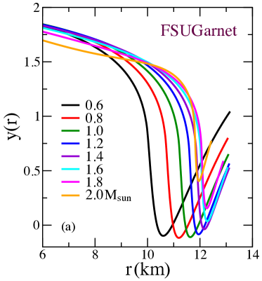
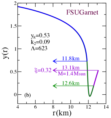
Figure 2: (Color online) (a) The $y(r)$ profile as defined in Eq. (12) for a variety of neutron-star masses as predicted by FSUGarnet Chen and Piekarewicz (2015). The Love number is sensitive to $y_{\raisebox{-0.75pt}{\tiny{\rm R}}}$, namely, the value of $y(r)$ at the surface of the star. (b) Same as in (a) but now exclusively for a $1.4\,M_{\odot}$ neutron star with special emphasis on the contribution to $y(r)$ from various regions of the star.

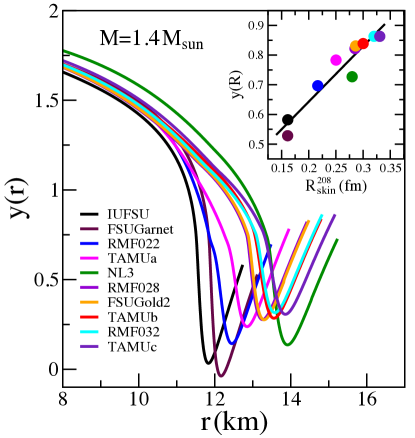
Figure 3: (Color online) The $y(r)$ profile as defined in Eq. (12) for a $1.4\,M_{\odot}$ neutron star as predicted by a collection of ten relativistic models with different choices for the density dependence of the symmetry energy. The inset shows a correlation between $y_{\raisebox{-0.75pt}{\tiny{\rm R}}}\!=\!y(R)$ and the neutron skin thickness of ²⁰⁸Pb that is used as proxy for the slope of the symmetry energy $L$.

In Fig. 2(a) we show the entire function $y(r)$ for a range of neutron-star masses as predicted by “FSUGarnet”, an accurately-calibrated relativistic model that accounts for known properties of atomic nuclei and neutron stars Chen and Piekarewicz (2015). The function starts at $y(0)\!=\!2$ and decreases smoothly beyond $r\!=\!0$ until it reaches the outer stellar region where it changes rapidly and becomes non-monotonic. This characteristic shape is independent of the stellar mass, although changes in the function become more pronounced with increasing mass. To better illustrate this behavior—and to underscore the role of the stellar crust—we isolate in Fig. 2(b) the profile associated with a $1.4\,M_{\odot}$ neutron star. The EOS in the uniform liquid core dominates up to nearly 12 km, or about 90%, of the radius of the star. Over this region $y(r)$ is relatively smooth and its value drops from $y(0)\!=\!2$ at the origin to about 0.75. Beyond this region the uniform ground state becomes unstable to cluster formation and the solid crust develops. The $11.8\!-\!12.6\,{\rm km}$ region comprises the entire inner crust and it is here where the function displays its entire non-monotonic behavior. Over this region $y(r)$ drops below zero and “heals” to a value of 0.19 at the interface between the inner and outer crust. The behavior of $y(r)$ in the outer crust is fairly smooth and yields its final value of $y_{\raisebox{-0.75pt}{\tiny{\rm R}}}\!=\!0.53$. Knowledge of both the compactness parameter $\xi$ and $y_{\raisebox{-0.75pt}{\tiny{\rm R}}}$ is sufficient to determine the second Love number $k_{2}\!=\!0.091$ and ultimately the tidal polarizability $\Lambda_{1.4}\!=\!623$. We note in passing that the value of the tidal polarizability reported here is consistent with the limit extracted from GW170817 and reported in the original discovery paper Abbott et al. (2017). However, in a more recent analysis that assumes that both colliding bodies are neutron stars that are described by the same equation of state, the limit on the tidal polarizability becomes even more stringent: $\Lambda_{1.4}\!=\!190^{+390}_{-120}$ Abbott et al. (2018). This result favors soft equations of state, perhaps even softer than the already soft FSUGarnet EOS. Moreover, it strengthens the argument presented in Ref. Fattoyev et al. (2018) that suggests that if the upcoming PREX-II measurements confirms that the neutron skin thickness of ²⁰⁸Pb is large Abrahamyan et al. (2012); Horowitz et al. (2012), this may be evidence of a softening of the symmetry energy at high densities—likely indicative of a phase transition in the stellar interior.

We end this section by displaying in Fig. 3 $y(r)$ for a $1.4\,M_{\odot}$ neutron star as predicted by a collection of relativistic models that, while accurate in their predictions of nuclear ground-state properties, differ significantly in the behavior of the poorly-known density dependence of the symmetry energy Lalazissis et al. (1997, 1999); Fattoyev et al. (2010); Fattoyev and Piekarewicz (2013); Chen and Piekarewicz (2014, 2015). The inset in the figure shows $y_{\raisebox{-0.75pt}{\tiny{\rm R}}}$ as a function of the neutron skin thickness of ²⁰⁸Pb, which is a good proxy for the density dependence of the symmetry energy. In summary, we conclude that whereas the stellar crust plays a minor role in the determination of the radius of the star and even less so in the determination of the mass, it greatly influences the shape of the entire profile $y(r)$ and particularly its value at the surface $y_{\raisebox{-0.75pt}{\tiny{\rm R}}}$. Moreover, one should remember that the inner crust, the region in which the behavior of $y(r)$ is no longer monotonic, is believed to harbor the nuclear-pasta phase, an exotic state of matter with an equation of state that is presently uncertain. Thus, it is critical to quantify uncertainties in the second Love number that originate from the various choices adopted for the EOS in the inner crust.

III.2 The (in)sensitivity of the tidal polarizability to the EOS of the inner crust

As mentioned earlier in Sec. II.1.3, the complexity of the inner stellar crust has hindered the construction of a detailed EOS and has made us rely on a cubic interpolation between the solid outer crust and the uniform liquid core. It was shown in Ref. Piekarewicz et al. (2014) that the “crustal radius” displays a strong sensitivity to the EOS of the inner crust. We define the crustal radius as the $\sim\!1$ km component of the entire stellar radius residing in the crust. In this section we examine the impact of the crustal EOS on $y_{\raisebox{-0.75pt}{\tiny{\rm R}}}$, $k_{2}$, and $\Lambda$. For simplicity, we choose an EOS for the inner crust of the form $P({{\varepsilon}})=A+B{{\varepsilon}}^{\gamma}$ Link et al. (1999); Carriere et al. (2003), using three different polytropic indices: $\gamma\!=\!1$, $4/3$, and $2$.

$\gamma$	$R_{\rm crust}$	$R$	$\xi$	$y_{\raisebox{-0.75pt}{\tiny{\rm R}}}$	$k_{2}$	$\Lambda$
$1.0$	$1.402$	$13.246$	$0.312$	$0.600$	$0.087$	$623.7$
$4/3$	$0.985$	$12.828$	$0.322$	$0.342$	$0.102$	$623.1$
$2.0$	$0.755$	$12.598$	$0.328$	$0.185$	$0.111$	$623.2$

Table 1: Predictions for the crustal radius, total stellar radius, compactness parameter $\xi$, $y_{\raisebox{-0.75pt}{\tiny{\rm R}}}$, Love number $k_{2}$, and dimensionless tidal polarizability $\Lambda$ as a function of the polytropic index $\gamma$ for a $1.4M_{\odot}$ neutron star. Both the crustal and total radii are given in kilometers and the EOS for the uniform liquid core is as predicted by the FSUGarnet model Chen and Piekarewicz (2015).

In Table 1 we examine the impact of the choice of polytropic index $\gamma$ on the crustal and total stellar radii, $\xi$, $y_{\raisebox{-0.75pt}{\tiny{\rm R}}}$, $k_{2}$, and $\Lambda$ for a $1.4M_{\odot}$ neutron star. For all three values of $\gamma$ the EOS for the uniform liquid core is the one predicted by the FSUGarnet model Chen and Piekarewicz (2015). As is evident from these results, the EOS for the inner crust is important in the determination of all these quantities—except for the dimensionless tidal polarizability $\Lambda$. This surprising result emerges from an unexpected cancellation between the second Love number $k_{2}$ and the stellar compactness parameter $\xi$. Whereas $\Lambda$ depends on both $\xi$ and $k_{2}$, with $k_{2}$ a highly complex function of $\xi$ and $y_{\raisebox{-0.75pt}{\tiny{\rm R}}}$ [see Eq.(10)], the product $k_{2}\,\xi^{-5}\!\propto\Lambda$ is equal for all three values of $\gamma$ to better than 0.1%. So while the second Love number is highly sensitive to the crustal component of the EOS, such sensitivity disappears in the case of the tidal polarizability, whose behavior, as we show in the next section, is largely dictated by the EOS of the uniform liquid core. This is not to say that the stellar crust plays no role in the determination of $\Lambda$. Quite the contrary, a 1-2 km contribution from the crust to the stellar radius is critical. What we have concluded is that “reasonable” changes to the EOS of the inner crust have no impact on the value of tidal polarizability.

III.3 Tidal polarizability and stellar compactness

Having examined the sensitivity of the second Love number $k_{2}(\xi,y_{\raisebox{-0.75pt}{\tiny{\rm R}}})$ to the underlying EOS—particularly to the crustal component—we now proceed to explore the model dependence of the tidal polarizability $\Lambda$ defined in Eq. (9). We start by displaying in Fig. 4(a) predictions for the mass-radius relation from a representative set of RMF models that span a relatively wide range of neutron star radii. All these models are successful in reproducing well-measured laboratory observables and, as indicated in the figure, consistent with the $M_{\star}\!\simeq\!2\,M_{\odot}$ limit for the maximum stellar mass Demorest et al. (2010); Antoniadis et al. (2013). Moreover, because of its relativistic character, they provide a Lorentz covariant extrapolation to dense matter that ensures that the speed of sound remains below the speed of light at all densities. For reference, the ten models adopted in this contribution are: NL3 Lalazissis et al. (1997, 1999), IU-FSU Fattoyev et al. (2010), TAMUC-FSU Fattoyev and Piekarewicz (2013), FSUGold2 Chen and Piekarewicz (2014), and FSUGarnet together with three parametrizations denoted by RMF022, RMF028, and RMF032 Chen and Piekarewicz (2015). Note that each model is labeled by the predicted value of the neutron skin thickness of ²⁰⁸Pb, which is a faithful proxy for the slope of the symmetry energy. Indeed, the larger the neutron neutron skin thickness of ²⁰⁸Pb, the larger the stellar radius Horowitz and Piekarewicz (2001a, b). Note that in a recent analysis of the tidal polarizability extracted from GW170817 Abbott et al. (2017), we used these same ten models to infer upper limits on both the radius of a $M_{\star}\!=\!1.4\,M_{\odot}$ neutron star and the neutron skin thickness of ²⁰⁸Pb: $R_{1.4}\!\lesssim\!13.76$ km and $R_{\rm skin}^{208}\!\lesssim\!0.25$ km Fattoyev et al. (2018), respectively. For every mass-radius combination predicted by a given EOS, one solves for the axially-symmetric quadrupole field at the stellar surface $y_{\raisebox{-0.75pt}{\tiny{\rm R}}}$, as indicated in the Appendix. From these three quantities ($R$, $M$, and $y_{\raisebox{-0.75pt}{\tiny{\rm R}}}$) both the second Love number $k_{2}$ and the dimensionless tidal polarizability $\Lambda$ can be computed. Having done so, we display in Fig. 4(b) the tidal polarizability as a function of both the stellar mass and stellar radius as predicted by the various equations of state. In particular, we indicate with an arrow the upper limit of $\Lambda_{1.4}\!\leq\!800$ extracted from the original discovery paper Abbott et al. (2017); this upper limit decreases even further if one adopts the revised analysis presented in Ref. Abbott et al. (2018). Indicated with circles of the appropriate color is the location of a $M_{\star}\!=\!1.4\,M_{\odot}$ neutron star. Although slightly difficult to discern in this logarithmic scale, only the four models with the softest symmetry energy—and thus predicting the four most compact configurations—remain consistent with the $\Lambda_{1.4}\!\leq\!800$ limit; see also Fig.4 in Ref. Fattoyev et al. (2018).

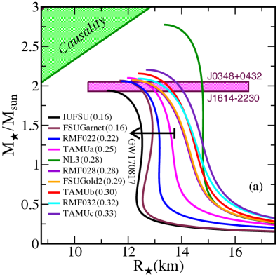
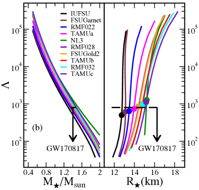
Figure 4: (Color online) (a) Mass-Radius relationship predicted by the ten models of the equation of state discussed in the text. Mass constraints from Demorest et al. (2010); Antoniadis et al. (2013) are indicated with a combined uncertainty bar and the radius constraint by an arrow as in Ref. Fattoyev et al. (2018). The excluded causality region was adopted from Ref. Lattimer and Prakash (2007). (b) The dimensionless tidal polarizability as a function of both the stellar mass and radius. The arrows indicate constraints inferred from the $\Lambda\!\leq\!800$ limit for a $1.4\,M_{\odot}$ neutron star Abbott et al. (2017). In turn, the colored circles indicate the corresponding predictions for the location of a $1.4\,M_{\odot}$ neutron star.

As alluded earlier in Sec. II.2, the tidal polarizability is a very sensitive function of the compactness parameter $\xi$. Scaling as the fifth power of $\xi$, a change in the stellar radius from 12 km to 14 km leads to an increase in $\Lambda$ by more than a factor of two; see Fig. 4(b). However, although often used as a constraint on stellar radii, the tidal polarizability is not an independent function of the mass and the radius. Rather, the dimensionless tidal polarizability scales as the dimensionless ratio of the stellar mass to the stellar radius $\xi\!\equiv\!R_{s}/R\!=\!2GM/c^{2}R$. There are, of course, scaling violations to $\Lambda$ encoded in the second Love number $k_{2}$ which although sensitive to $\xi$, also depends on the entire equation of state through its dependence on the quadrupole field at the stellar surface $y_{\raisebox{-0.75pt}{\tiny{\rm R}}}$; see Eq. (10). However, for a given compactness parameter $\xi$, the dependence of $k_{2}$ on $y_{\raisebox{-0.75pt}{\tiny{\rm R}}}$ is relatively mild—at least for the set of models considered in this work. The model dependence of $k_{2}$ on the EOS is displayed in Fig. 5(a) as a function of the compactness parameter $\xi$. The failure of all predictions to collapse into one single curve is due to their dependence on $y_{\raisebox{-0.75pt}{\tiny{\rm R}}}$. Nevertheless, the model dependence is mild, with the largest difference between models being of the order of 25%. Yet such mild model dependence all but disappears as one plots the dimensionless tidal polarizability $\Lambda$ as a function of the compactness parameter $\xi$. That in this case all ten predictions collapse into a single curve is due to the $\xi^{-5}$ scaling of $\Lambda$; see Fig. 5(b) where $\Lambda$ is plotted using both logarithmic and linear scales. For example, assuming a dimensionless tidal polarizability of $\Lambda_{\star}\!=\!800$, results in theoretical predictions from all ten models that fall within the very narrow range of $0.29\lesssim\!\xi\!\lesssim 0.30$. Fig. 5(b) demonstrates that an accurate measurement of the dimensionless tidal polarizability fixes the stellar compactness. This kind of “universal” relation among various stellar observables is reminiscent of the “I-Love-Q” relations explored extensively by Yagi and Yunes to project out any uncertainties in nuclear physics Yagi and Yunes (2013a, b, 2017). In this context our aim is rather different. Our goal is to actually confront these nuclear physics uncertainties by combining laboratory experiments and astrophysical observations in an effort to determine the EOS. Yet, in an effort to generate the entire mass-radius relationship from which the neutron-star matter EOS may be uniquely determined Lindblom (1992), additional stellar observables that are sensitive to a different combination of masses and radii must be measured. In the context of binary neutron star mergers, the “chirp” mass and the “reduced” tidal polarizability Flanagan and Hinderer (2008); Favata (2014) offer an attractive alternative.

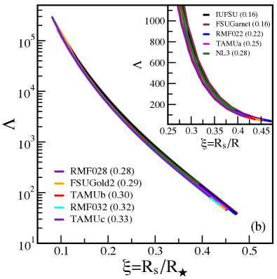
Figure 5: (Color online) (a) The second tidal Love number $k_{2}$ as a function of the compactness parameter $\xi$ as predicted by the ten models of the equation of state used in the text. Although $k_{2}$ depends on $\xi$, the failure of all predictions to collapse into a single curve is due to its dependence on $y_{\raisebox{-0.75pt}{\tiny{\rm R}}}$, which in turns depends on the entire EOS. (b) Same as (a) but now for the dimensionless tidal polarizability $\Lambda$. The collapse of all ten predictions into a universal curve is due to the strong sensitivity of $\Lambda$ to the compactness parameter $\xi$.

IV Conclusions

The brand new era of multimessenger astronomy started on August 17, 2017 with the first direct detection of both gravitational and electromagnetic radiation from the binary neutron star merger GW170817. GW170817 established for the first time the association of short gamma ray bursts with neutron star mergers and the critical role that the radioactive decay of $r$-process elements plays in powering the kilonova light curve. Moreover, GW170817 has started to provide fundamental new insights into the nature of dense matter by adding the tidal polarizability to the arsenal of observables that inform the equation of state. Similar to the electromagnetic response of a polar molecule to the presence of an external electric field, the tidal polarizability encodes the response of the neutron star to the external tidal field produced by its companion. Given that the tidal polarizability “hides” within a high order coefficient in the post-Newtonian expansion of the gravitational wave form, its extraction becomes a challenging proposition. As such, GW170817 could only established upper limits on the tidal polarizability of a 1.4 solar mass neutron star. Nevertheless, these limits are already stringent enough to rule out equations of state that predict relatively large stellar radii.

Besides its sensitivity to the stellar compactness, the tidal polarizability depends on the second tidal Love number $k_{2}$. Particularly relevant to the determination of $k_{2}$ is the value of the logarithmic derivative of the non-spherical (quadrupole) component of the gravitational potential at the stellar surface $y_{\raisebox{-0.75pt}{\tiny{\rm R}}}\!\equiv\!y(r\!=\!R)$, a quantity that emerges from solving a non-linear differential equation that is highly sensitive to the underlying equation of state. Although the value of $y_{\raisebox{-0.75pt}{\tiny{\rm R}}}$ (and the compactness parameter) is all that is needed to compute $k_{2}$, we found that the underlying function $y(r)$ displays an interesting structure. In particular, $y(r)$ displays a non-monotic behavior that is entirely controlled by the equation of state in the inner stellar crust. Given that the inner crust is characterized by the emergence of complex topological structures collectively known as nuclear pasta, the equation of state in this region is poorly known. So despite the fact that the inner crust typically accounts for less than 10% of the stellar radius, its impact on the determination of $k_{2}$ was found to be significant. Whereas $y(r)$ falls smoothly and monotonically over the uniform stellar core, its behavior in the inner crust is neither monotonic nor smooth. Indeed, $y(r)$ attains its minimum value (often negative) in the inner crust to then rise monotonically over the dilute regions of the inner crust and over the entire outer crust. How will this behavior be modified, if any, with a more realistic description of the EOS in the inner crust provides one more reason to elucidate the fascinating and complex dynamics of the Coulomb frustrated nuclear pasta. Nevertheless, we found that due to an unexpected cancellation between $k_{2}$ and the stellar compactness $\xi$, “reasonable” modifications to the EOS of the inner stellar crust have no impact on the tidal polarizability.

In summary, we have examined in considerable detail the sensitivity of the second tidal Love number to the neutron star matter equation of state. For a fixed compactness parameter, $k_{2}$ is the only component of the tidal polarizability sensitive to the underlying EOS, particularly to the contribution from the inner stellar crust. Given that the tidal polarizability scales as the fifth power of the compactness parameter, $k_{2}$ provides a small correction to the scaling relation between $\Lambda$ and the compactness parameter. Yet the multimessenger era is in its infancy and many more detections of binary neutron star mergers are anticipated as LIGO-Virgo prepares for its third observing run, likely to start at the beginning of 2019. Also in 2019, PREX-II will provide significantly improved limits on the neutron skin thickness of ²⁰⁸Pb which, in turn, will constrain the EOS in the vicinity of saturation density. We are confident that PREX-II in conjunction with the increased sensitivity of gravitational wave detectors will provide critical information on individual stellar masses and tidal polarizabilities. This powerful synergy will yield a determination of the mass-radius relation and ultimately of the underlying equation of state.

*

Appendix A The Love Number

As shown in Eq. (9), once the TOV equations are solved and the compactness parameter $\xi$ has been extracted, the only remaining unknown in the computation of the tidal polarizability is the second Love number $k_{2}(\xi,y_{\raisebox{-0.75pt}{\tiny{\rm R}}})$. In this Appendix we outline the steps necessary to compute $y_{\raisebox{-0.75pt}{\tiny{\rm R}}}$.

We start by invoking a Newtonian description of the static gravitational potential in terms of two non-spherical contributions: (i) an external tidal field (perhaps produced by the companion) plus (ii) an induced stellar contribution in response to the external tidal field. One assumes that the external gravitational potential is slowly varying over the dimensions of the star so that it may be expanded in a Taylor series around its center, assumed to be the origin. The external gravitational potential at an observation point ${\bf r}$ in the stellar neighborhood may then be written as

$$\Phi_{\rm ext}({\bf r})=\Phi_{\rm ext}(0)+{\bf r}_{i}\partial_{i}\Phi_{\rm ext}(0)+\frac{1}{2}{\bf r}_{i}{\bf r}_{j}\partial_{i}\partial_{j}\Phi_{\rm ext}(0)+\ldots=\Phi_{\rm ext}(0)+{\bf r}_{i}\partial_{i}\Phi_{\rm ext}(0)+\frac{1}{2}{\mathcal{E}}_{ij}{\bf r}_{i}{\bf r}_{j}+\ldots$$ (13)

where the external tidal field has been defined as ${\mathcal{E}}_{ij}\!\equiv\!\partial_{i}\partial_{j}\Phi_{\rm ext}(0)$. Along the same lines, the induced gravitational potential at a point ${\bf r}$ outside the star may be expanded in a multipole series:

$$\Phi_{\rm ind}({\bf r})=-G\left(\frac{M}{r}+\frac{{\bf p}_{i}{\bf r}_{i}}{r^{3}}+\frac{1}{2}Q_{ij}\frac{{\bf r}_{i}{\bf r}_{j}}{r^{5}}+\ldots\right),$$ (14)

where ${\bf p}$ and $Q_{ij}$ are the dipole and quadrupole moments of the stellar distribution, namely,

$${\bf p}=\int\!{\bf r}\rho({\bf r})d^{3}r\hskip 5.0pt{\rm and}\hskip 5.0ptQ_{ij}=\int\!\Big{(}3{\bf r}_{i}{\bf r}_{j}-r^{2}\delta_{ij}\Big{)}\rho({\bf r})d^{3}r.$$ (15)

Unlike the electric dipole moment of a charge distribution, the dipole moment of a mass distribution can always be made to vanish by placing the origin at the center of mass. Moreover, given that the gravitational potential is defined up to an overall constant and that the second term in Eq. (13) induces an overall translation of the center of mass, the overall gravitational potential may be written as

$$\Phi({\bf r})=\Phi_{\rm ind}({\bf r})+\Phi_{\rm ext}({\bf r})=-G\left(\frac{M}{r}+\frac{1}{2}Q_{ij}\frac{{\bf r}_{i}{\bf r}_{j}}{r^{5}}+\ldots\right)+\frac{1}{2}{\mathcal{E}}_{ij}{\bf r}_{i}{\bf r}_{j}+\ldots$$ (16)

In the context of general relativity, the gravitational potential of a Schwarzschild star—namely, a spherical, static, and relativistic star described by the TOV equations—is directly related to the “tt-component” of the metric tensor. That is,

$$g_{tt}(r)\!=\!-e^{2\Phi(r)}\,\xRightarrow[\Phi\ll 1]{}-1-2\Phi(r)+\ldots,$$ (17)

In the presence of a gravitational field with non-spherical components that are treated in the linear regime, the Schwarzschild metric is suitably modified as follows Hinderer (2008):

$$g_{tt}(r,\theta,\phi)=-e^{2\Phi(r)}\Big{(}1+H(r)Y_{20}(\theta,\varphi)\Big{)},$$ (18)

where only an axially-symmetric external quadrupole field is considered and $H(r)$ satisfies a linear, homogeneous, second-order differential equation Hinderer (2008); Hinderer et al. (2010); Postnikov et al. (2010):

$$\frac{d^{2}H(r)}{dr^{2}}+\left(\frac{1+F(r)}{r}\right)\frac{dH(r)}{dr}+Q(r)H(r)=0,\hskip 10.0pt{\rm with}\;\lim_{r\rightarrow 0}H(r)\simeq r^{2}.$$ (19)

Note that the relevant bilinear product of ${\bf r}$ written in cartesians coordinates in Eq. (16) is related to the azimuthally independent ($l\!=\!2,m\!=\!0$) spherical harmonic:

$$\big{(}{\bf r}\otimes{\bf r}\big{)}_{20}=\frac{1}{\sqrt{6}}\Big{(}3z^{2}-r^{2}\Big{)}=\sqrt{\frac{8\pi}{15}}\hskip 2.0ptr^{2}Y_{20}(\theta,\varphi).$$ (20)

Also note that both $F(r)$ and $Q(r)$ given in Eq. (19) are known functions of the mass, pressure, and energy density profiles assumed to have been obtained previously by solving the TOV equations and are give by the following expressions Fattoyev et al. (2013):

$$F(r)=\frac{1-4\pi Gr^{2}\Big{(}{{\varepsilon}}(r)-P(r)\Big{)}}{\displaystyle{\left(1-\frac{2GM(r)}{r}\right)}},$$ (21)

$$Q(r)=\frac{4\pi}{\displaystyle{\left(1-\frac{2GM(r)}{r}\right)}}\left(5{{\varepsilon}}(r)+9P(r)+\displaystyle{\frac{{{\varepsilon}}(r)+P(r)}{{c}_{\rm s}^{2}(r)}}-\frac{6}{4\pi r^{2}}\right)-4\left[\frac{G\Big{(}M(r)+4\pi r^{3}P(r)\Big{)}}{\displaystyle{r^{2}\left(1-\frac{2GM(r)}{r}\right)}}\right]^{2},$$ (22)

where ${c}_{\rm s}^{2}(r)\!=\!dP(r)/d{{\varepsilon}}(r)$ is the speed of sound at a depth $r$.

In principle, this is sufficient to compute $y_{\raisebox{-0.75pt}{\tiny{\rm R}}}$, that is obtained from the logarithmic derivative of $H(r)$ evaluated at the surface of the star Hinderer (2008), namely,

$$y_{\raisebox{-0.75pt}{\tiny{\rm R}}}=y(r\!=\!R)\equiv\left(\frac{d\ln H(r)}{d\ln r}\right)_{\!r=R}=\left(\frac{rH^{\prime}(r)}{H(r)}\right)_{\!r=R}.$$ (23)

However, given that all that is needed to compute the Love number is $y_{\raisebox{-0.75pt}{\tiny{\rm R}}}$, it was suggested in Ref. Postnikov et al. (2010) that perhaps solving directly for $y(r)$ may be more efficient than solving for $H(r)$. That is, by introducing the following transformation,

$$y(r)\equiv\left(\frac{rH^{\prime}(r)}{H(r)}\right)\iff H(r)=H(r_{0})\exp\left(\int_{r_{0}}^{r}\frac{y(r^{\prime})}{r^{\prime}}dr^{\prime}\right),$$ (24)

it is easy to show that the function $y(r)$ satisfies the following first-order—albeit non-linear—differential equation:

$$r\frac{dy(r)}{dr}+y^{2}(r)+F(r)y(r)+r^{2}Q(r)=0,\hskip 10.0pt{\rm with}\;y(0)=2.$$ (25)

In this way $y_{\raisebox{-0.75pt}{\tiny{\rm R}}}$ is directly obtained from the value of the function $y(r)$ evaluated at $r\!=\!R$.