Self-Attention Equipped Graph Convolutions for Disease Prediction

Abstract

Multi-modal data comprising imaging (MRI, fMRI, PET, etc.) and non-imaging (clinical test, demographics, etc.) data can be collected together and used for disease prediction. Such diverse data gives complementary information about the patient’s condition to make an informed diagnosis. A model capable of leveraging the individuality of each multi-modal data is required for better disease prediction. We propose a graph convolution based deep model which takes into account the distinctiveness of each element of the multi-modal data. We incorporate a novel self-attention layer, which weights every element of the demographic data by exploring its relation to the underlying disease. We demonstrate the superiority of our developed technique in terms of computational speed and performance when compared to state-of-the-art methods. Our method outperforms other methods with a significant margin.

Index Terms—  Multi-modal, Graph Convolutions, Disease prediction

1 Introduction

Experts look at all the varied multi-modal data collected by imaging sources and non-imaging demographics (age, gender, weight, body-mass index) to take an informed decision for disease diagnosis. Such rich data is also exploited in Computer Aided Diagnosis systems (CADs) as complementary information. Current CAD systems combine all the complementary features by using feature selection [1], or by reducing the dimensionality with an autoencoder [2, 3, 4]. Works are also done with simply concatenating all the features to use deep learning based models [5]. All the above methods exploit the complementary information from available modalities at a global level but fail to optimally combine the varied information. For instance, the learned features are biased towards the single modality with dominant features and do not exploit the individuality of each modality. On top of that, each demographic information carries different relevance for the diagnosis of a disease. A model is required which is capable of evaluating the significance of every element of the demographic data and performing the prediction task based on the selective and weighted procedure for elements of demographic data. Such a scheme will boost the disease prediction task to incorporate more clinical semantics.

Graphs provide a more such a way of using multi-modal data [6, 7]. These methods leverage the similarities between subjects in terms of an affinity graph in the training process itself. Most recent work [6] by presents an intelligent and novel use case of Graph Convolutional Networks (GCN) for the binary classification task. This allows convolutions to be used on graph-structured data, where each patient represents a node in the population level graph. The method proposes to use each demographic information separately to construct a neighborhood graph. They eventually combine all the neighborhood graphs to get the average affinity graph, unlike the conventional methods, which fuses the information for the prediction task. This method, however, yields varied results for distinct input neighborhood graphs. Each of these affinity graphs and indirectly each element of the demographic data carries distinct neighborhood relationships (based on element dependent criteria) and statistical properties with respect to the entire population.

Our motivation is to analyze the impact and relevance of the neighborhood definitions on the final task of disease prediction. In addition to that, we want to investigate whether the relative weighting of meta-data can be automated. Contributions: 1) We propose a model capable of incorporating the information of each graph separately, 2) our design architecture bears a parallel setting of Graph Convolutional (GC) layers 3) we introduce a ’Self-Attention layer’ which automatically learns the weighting for each meta-data with respect to its relevance to the prediction task, and 4) Our model outperforms the state-of-the-art method.

2 Methodology

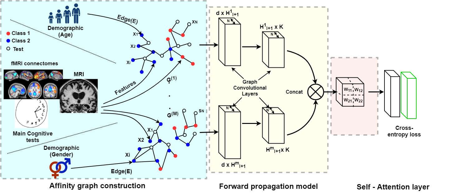
Fig. 1: Figure describes the Multi-Layered Parallel Graph Convolutional Network with $M$=2. Two branches have same input features but input affinity matrix.

Given a dataset $\mathcal{D}=\{X,Y,\delta\}$ with $X\in\mathbb{R}^{N\times d}$ representing the feature matrix for $N$ patients and each one is provided with $d$-dimensional features. $Y$ represents the corresponding label matrix and $\delta$ the demographic data matrix. The task is to predict the class label $\hat{Y}$ for test subjects for $K$ classes. $\delta\in\mathbb{R}^{N\times M}$ represents that for each patient $M$-dimensional demographic data is provided. The $m^{th}$ affinity graphs $G^{(m)}\in\mathbb{R}^{N\times N}$ are computed from the respective $\delta^{m}$ demographic element. The model $f(\cdot)$ to solve the task is given by

$$\hat{Y}=f(X,G^{(m)};\theta).$$ (1)

The model takes $X$ and $G^{(m)}$ as input to train the parameters $\theta$ and outputs discriminative features for classification. Fig. 1 shows the entire methodology, which can be divided into three main parts: (1) Affinity matrix $W^{m}$ construction, (2) the forward propagation model: we describe the model, where architecture to produce class-separable features and (3) the self-attention layer, for automatic weighting of the graph-specific output features of each branch.
Affinity Matrix $W^{(m)}$ Construction: We construct $M$ affinity matrices corresponding to each of the demographic element. For the $m^{th}$ element, let the graph $G^{(m)}=\left\{X,E^{(m)}\right\}$ be an undirected and unweighted, where all the $M$ graphs have a common vertex set $X$. $E^{(m)}\in\mathbb{R}^{N\times N}$ is a demographic element specific edge matrix. Each graph $G^{(m)}$ reveals distinct intrinsic relationships between the vertices. Edges between vertices are defined based on the given demographic element as

$$E^{(m)}_{i,j}=\begin{cases}1&if\left|\delta_{i,m}-\delta_{j,m}\right|<\beta\\ 0&otherwise\end{cases},$$ (2)

where $\delta^{m}(\cdot)$ is the corresponding demographic element and $\beta$ is a threshold. We generate affinity matrix from these graphs by weighting the edges. A similarity metric between the subjects $Sim(X_{i},X_{j})$, e.g. correlation coefficient, is incorporated to weight the edges as

$$W^{(m)}_{i,j}=Sim(X_{i},X_{j})\circ E^{(m)}_{i,j}\left(X_{i},X_{j}\right),$$ (3)

where $\circ$ is the Hadamard product.
Forward propagation model: We design our model such that it trains each affinity graph separately. The proposed model bears the parallel setting of $M$ branches as shown in Fig. 1. Each branch is equipped with spectral graph theory based GC layers. These layers help to adopt convolutions on graphs unlike grid based convolutions  [7, 8]. The proposed forward propagation model is given by:

$$H_{l+1}^{(m)}=\sigma\left({D^{(m)}}^{-\frac{1}{2}}W^{(m)}{D^{(m)}}^{-\frac{1}{2}}H_{l}^{(m)}\Theta_{l}^{(m)}\right)$$ (4)

$D$ is the diagonal matrix with $D_{ii}^{(m)}=\sum_{j}W_{ij}^{(m)}$. $\Theta_{l}^{(m)}$ are the trainable layer-specific filters, which can be derived from a first-order approximation of localized spectral filters on graphs [7], and $H_{l}^{(m)}$ is the feature representation of the previous layer ($H_{0}^{(m)}=X$). ${D^{(m)}}^{-\frac{1}{2}}W^{(m)}{D^{(m)}}^{-\frac{1}{2}}$ is the normalized graph Laplacian, and $\sigma(\cdot)$ is the rectified linear unit function. The model outputs $H_{logits}\in\mathbb{R}^{N\times K}$.

Self-Attention Layer: The logits for $M$ branches differ with respect to each other because of graphs although features on each vertex are common. In order to rank the demographic data elements, we design a linear combination layer that ranks the logits coming from the last hidden layer as

$$\hat{Y}=Softmax\left(\sum_{m=1}^{M}\omega_{m}H^{(m)}_{logits}\right),$$ (5)

where $\omega_{m}$ is the trainable scalar weight associated with the demographic element and $\hat{Y}$ are the normalized log probabilities. We define our objective function as binary weighted cross entropy loss on the labeled data to train the model parameter.

3 Experiments

Our experiments have been designed to (1) investigate the influence of each affinity matrix on the performance of the predictive models, (2) investigate the performance of the predictive model with multi-graph setting approaches [6], (3) we show comparison with 3 methods, linear classifier, two-layered Dense Neural Network, baseline GCN method [6], proposed model and (4) investigate in-depth insight of self-attention layer with multi-graph setting.
Dataset: We show results on a publicly available dataset namely Tadpole [9] for the prediction of Alzheimer's disease. The dataset is a subset of ADNI[10] consisting of 564 patients. The goal is to classify each patient into one of the three classes Normal, Mild Cognitive Impairment (MCI) and Alzheimer's disease (AD). For each patient, the features are collected from various biomarkers (MR, PET imaging, cognitive tests, CSF biomarkers, etc). Further risk factors are provided for each subject in terms of APOE genotyping status and FDG PET imaging. Demographic elements (age and gender) are also provided. Entire data is pre-processed with ADNI’s standard data-processing pipeline.Implementation: Number of features $d$ = 354, dropout rate: $0.3$, $\ell_{2}$- regularisation: $5\times 10^{-4}$. All the experiments are implemented in Tensorflow and performed with Nvidia GeForce GTX 1080 Ti 10 GB GPU. We use early stopping criteria to decide the number of epochs for each setting. The model is evaluated based on the classification mean accuracy (ACC) for 10-fold Cross-Validation.

4 Results and Discussion:

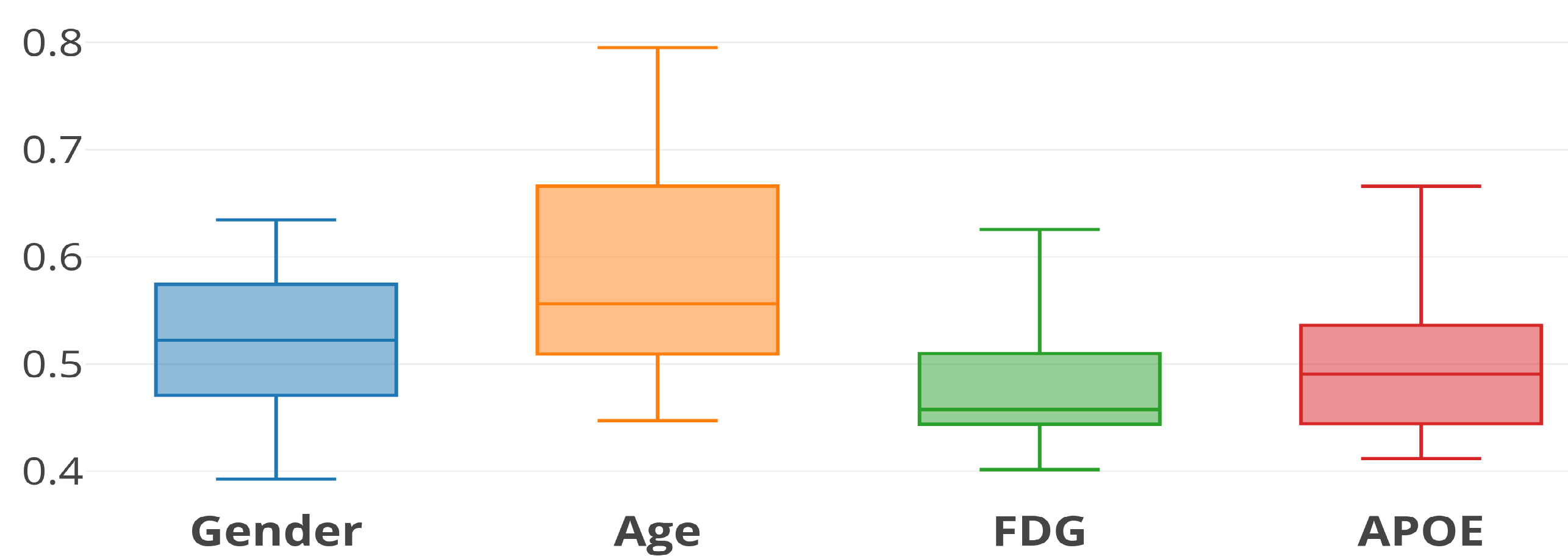
(a) Influence of individual affinity with each showing different mean accuracy matrix

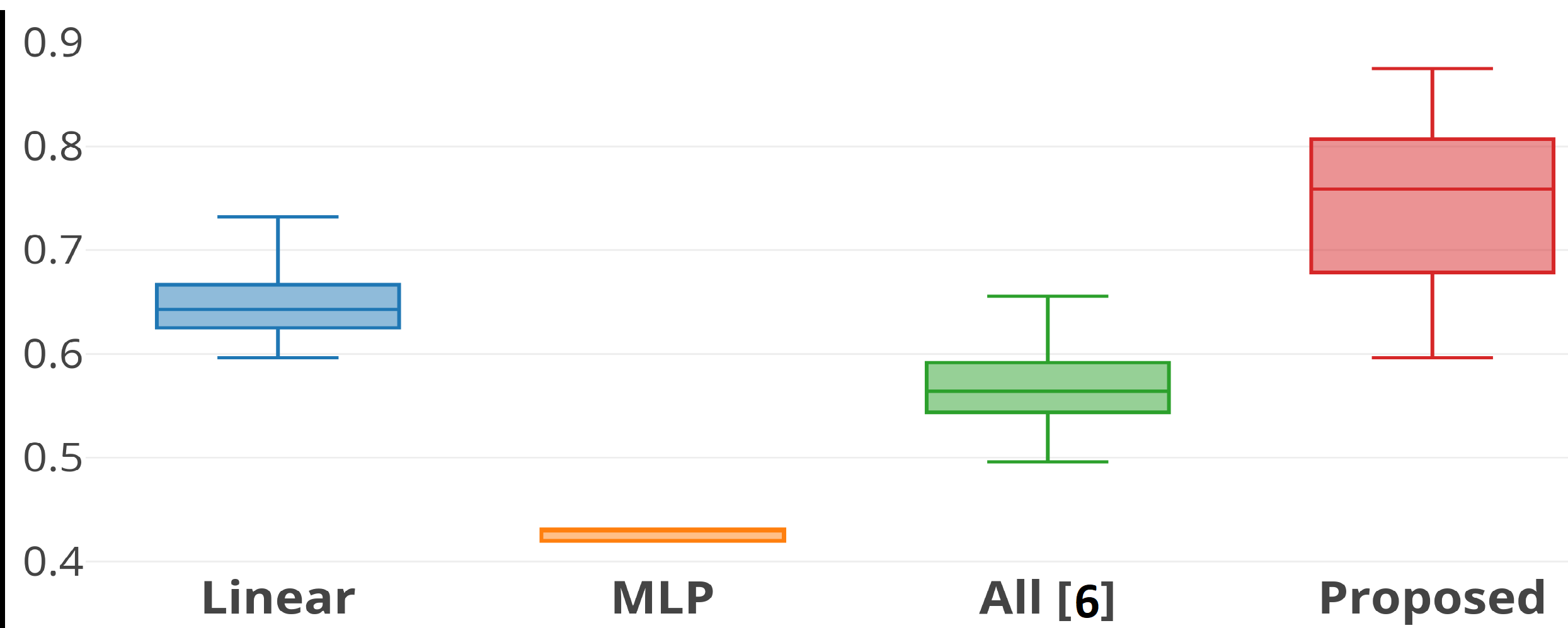
(b) The results over all the comparative methods with proposed model outperforming.

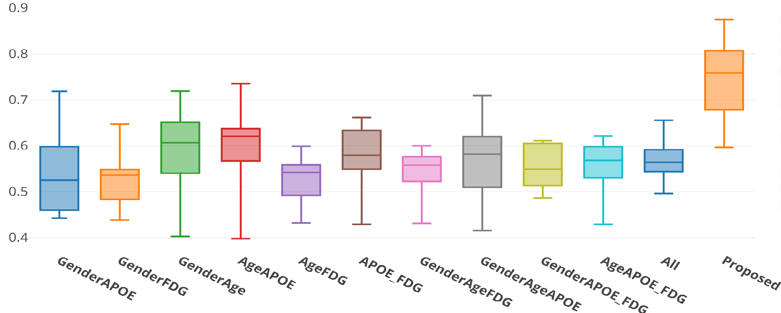
(c) Different combinations of all four affinity matrices showing differnt results

Fig. 2: All the three subfigures show the boxplots of accuracy over 10-folds cross validation.

In this section, we discuss the results of all the experiments in detail.
Influence of individual affinity matrix: For individual affinities it should be noted from fig. 2 (a) that each graph shows different results. This means that the input affinity matrices have unequal relevance to the task at hand. For example, the age graph shows the best performance and the FDG graph shows the worst. The performance reduces when all the graphs are averaged and used as input as in the baseline method [6]. This proves that averaging affinity graphs degrade the performance that could have been obtained otherwise.
Performance with different combinations of graphs: We perform another experiment by using all the different combinations of affinity matrices as input. This validates that the performance varies if the combination of affinity matrices is changed. According to [11] age and gender are the most important factors compared to APOE and FDG for the prediction of AD. The results are demonstrated in terms of boxplots of accuracies as shown in fig.2 (c) which confirms the different combination show different result.Moreover, the combination of gender and age show the maximum performance and most of the combinations using FDG and APOE reduce the performance. This depicts that our model upholds the clinical semantic same as [11]. This experiment also confirms that the overall performance reduces when all the affinity graphs are weighted equally and averaging deteriorates the positive influence of other affinity matrices due to the loss of neighborhood structure for individual graphs.Our proposed model with self-attention outperforms all the combinations, since it captures the correct weighting required for optimal performance.
Performance in comparison to other methods: We compare the proposed method to three state-of-the-art methods namely linear classifier, neural network and [6] as shown in fig. 2 (b). We chose these methods respectively to investigate 1) how linearly separable the features at every node are? 2) what is the performance of the model when features are concatenated? 3) what is the significance of incorporating the graph for the task? and 4) how important is it to weight the graphs? From fig. 2 (b), it can be seen that features are separable as the linear classifier performs quite well compared to two other methods shown. For NN, where the features are concatenated the model architecture becomes the problem. We used the same number of hidden layers (2) and hidden unties (16, 3 respectively) with the input of the feature dimension of 354. NN fails to perform well with this architecture. As can be seen that the baseline [6] improves the performance with respect to NN showing the strength of the GCN, however, it performs lower than linear and proposed. This is due to the corrupted combination of the neighborhood. Finally, our proposed method outperforms all the methods with the correct weighted combination of neighborhood and $H_{logits}$.
Effect of self attention: We also investigated the weights learnt for each branch by our model. The self-attention layer learned maximum weight for gender and age (0.35 and 0.27 respectively) and lower weight for FDG and APOE(0.09 and 0.29 respectively). It is confirmed from [11] that age and gender are significant factor for predicting AD.

5 Conclusion

All our experiments go inline with our hypothesis that affinity graphs influence the performance of disease prediction differently. GCNs are sensitive to the defined neighborhood. Combination of affinities alters the possible neighborhood between the subjects. Further, our proposed method with self-attention clearly incorporates the unequal contributions of graphs and outperforms all the setups with significant margin. The order of complexity for our model versus the baseline model [6] is nearly equal as $O(n)\approx O(2n)$, making it scalable for a larger number of demographic elements. We train the GC layers first for 150 epochs and then let the self-attention layer train further. This helps channelize the learning of weights of GC layers as well as self-attention layer. The features at every node are kept simpler to gain more insights about effect og graphs.

Further the choice of thresholds for creating the graphs are followed from clinical statistics provided by the literature. One might argue that splitting a single graph into multiple graphs will decrease the performance as some connections are lost in the thresholding process. However aggregating the graphs from different information source will lead to the loss of individual structure and unequal relevance cannot be considered.

References

- [1] Memarian et al., “Multimodal data and machine learning for surgery outcome prediction in complicated cases of mesial temporal lobe epilepsy,” Computers in biology and medicine, vol. 64, pp. 67–78, 2015.
- [2] Calhoun et al., “Multimodal fusion of brain imaging data: a key to finding the missing link (s) in complex mental illness,” BP:CNNI, vol. 1, no. 3, pp. 230–244, 2016.
- [3] Tiwari et al., “Multi-modal data fusion schemes for integrated classification of imaging and non-imaging biomedical data,” in Biomedical Imaging: From Nano to Macro, 2011 IEEE International Symposium on. IEEE, 2011, pp. 165–168.
- [4] Ngiam et al., “Multimodal deep learning,” in Proceedings of (ICML-11), 2011, pp. 689–696.
- [5] Tao Xu, Han Zhang, Xiaolei Huang, Shaoting Zhang, and Dimitris N Metaxas, “Multimodal deep learning for cervical dysplasia diagnosis,” in International Conference on MICCAI. Springer, 2016, pp. 115–123.
- [6] Parisot et al., “Spectral graph convolutions for population-based disease prediction,” in MICCAI. Springer, 2017, pp. 177–185.
- [7] Kipf et al., “Semi-supervised classification with graph convolutional networks,” arXiv preprint arXiv:1609.02907, 2016.
- [8] Defferrard et al., “Convolutional neural networks on graphs with fast localized spectral filtering,” in Adv Neural Inf Process Syst, 2016, pp. 3844–3852.
- [9] Marinescu et al., “Tadpole challenge: Prediction of longitudinal evolution in alzheimer’s disease,” arXiv preprint arXiv:1805.03909, 2018.
- [10] Jack Jr et al., “The alzheimer’s disease neuroimaging initiative (adni): Mri methods,” Journal of Magnetic Resonance Imaging: An Official Journal of the International Society for Magnetic Resonance in Medicine, vol. 27, no. 4, pp. 685–691, 2008.
- [11] Perrin et al., “Multimodal techniques for diagnosis and prognosis of alzheimer’s disease,” Nature, vol. 461, no. 7266, pp. 916, 2009.