Mapping the phase transitions of the ZGB model with inert sites via nonequilibrium refinement methods

Abstract

In this paper, we revisit the ZGB model and explore the effects of the presence of inert sites on the catalytic surface. The continuous and discontinuous phase transitions of the model are studied via time-dependent Monte Carlo simulations. In our study, we are concerned with building a refinement procedure, based on a simple concept known as coefficient of determination $r$, in order to find the possible phase transition points given by the two parameters of the model: the adsorption rates of carbon monoxide, $y$, and the density of inert sites, $\rho_{is}$. First, we obtain $10^{6}$ values of $r$ by sweeping the whole set of possible values of the parameters with an increment $10^{-3}$, i.e., $0\leq y\leq 1$ and $0\leq\rho_{is}\leq 1$ with $\Delta y=\Delta\rho_{is}=10^{-3}$. Then, with the possible phase transition points in hand, we turn our attention to some fixed values of $\rho_{is}$ and perform a more detailed refinement considering larger lattices and increasing the increment $\Delta y$ by one order of magnitude to estimate the critical points with higher precision. Finally, we estimate the static critical exponents $\beta$, $\nu_{\parallel}$, and $\nu_{\perp}$, as well as the dynamic critical exponents $z$ and $\theta$.

I Introduction

The production of carbon dioxide from catalytic surfaces is of fundamental interest from both scientific and technological points of view. In this context, one can consider the model devised by Ziff, Gulari, and Barshad ziff1986 in 1986 which, despite its simplicity, presents two different phase transitions: one continuous and another discontinuous. In addition, on the contrary of the continuous phase transition which seems to be only a theoretical prediction, the discontinuous one has been experimentally verified by several authors. The only parameter of the model is the adsorption rate of carbon monoxide molecules.

An important question that arises when studying such simple models is: How are the phase transitions affected by the inclusion of other parameters? As presented below, this question has been considered by several authors in recent years. For instance, some authors have included the diffusion of the adsorbed species (carbon monoxide molecules or oxygen atoms) on the catalystic surface jensen1990a ; Chan2015 ; buendia2015 ; Ewans1993 ; dasilva2018 , and others have studied the model with the desorption of molecules from the surface tome1993 ; albano1992 ; brosilow1992 ; kaukonen1989 ; fernandes2018 . In this paper, we include to the original model the existence of inert sites (or impurities) over the surface (see, for example, Ref. hoenicke2014 ). So, our intent is to analyse the two phase transitions of the original model when the adsorption rate and the density of inert sites vary. This study is focused on the use of a refinement method proposed for nonequilibrium Monte Carlo simulations in the context of short-time dynamics rather than the steady state Monte Carlo simulations. In Ref. dasilva2018 , we have shown that both continuous and discontinuous phase transitions are preserved when the diffusion of the adsorbed species are allowed. On the other hand, we have shown in Ref. fernandes2018 that the introduction of the desorption of carbon monoxide molecules from the lattice preserves the continuous phase transition and destroys the discontinuous one even for small values of desorption rates. In that same work, we have also shown that before the dissapearance of the discontinuous phase transition, there exists a sequence of “pseudocritical points” forming two lines that end in a single point. As predicted by Tomé and Dickman tome1993 , we have confirmed through the dynamic critical exponent $\theta$ that this is an Ising-like critical point.

In this paper, we are interested in showing how the insertion of the density of inert sites can affect the continuous and discontinuous phase transitions of the ZGB model. First, we analyze the behavior of the densities of CO and CO₂ molecules, of O atoms, and of vacant sites according to the two parameters of the model: the density of inert sites and the adsorption rate of CO molecules on the surface. To reach this goal, we consider a non-traditional way to explore such transitions. This approach, which was proposed in 2012 for generalized systems silva2012 , considers a refinement method based on a simple statistical concept known as coefficient of determination. It has been succesfully applied in models without defined Hamiltonian silva2015 ; fernandes2016 ; dasilva2018 ; fernandes2018 , in models with defined Hamiltonian and with short-range interactions silva2012 ; silva2013a ; silva2013b ; silva2014 ; fernandes2017 , and recently in long-range systems Longrange . With this method, we are able to obtain diagrams with the possible regions of phase transitions for the whole set of possible of values of adsorption rates and densities of inert sites of the model. After identifying the possible phase transitions points of the model through the coefficient of determination, we focused our attention to some determined points and refine our measurements in order to verify with good precision the influence of inert sites on the ZGB model. So, for the first time, the refinement process is carried out on two levels: at the first level, we consider a smaller lattice size and sweep all possible values of adsorption rates and densities of inert sites in order to obtain an overview of the phase transitions of the model; on the second level, we focus our attention only on the regions close to the phase transition points obtained previously in order to calculate the coefficient of determination for larger system sizes besides improving the precision of the measurements in one magnitude order (fine scale). Therefore, the process is even more precise than other previous explorations of the method. Finally, we calculate several critical exponents for some points in order to check the universality class of the model.

In the next section, we present the model to be studied and in Sec. III we briefly show the nonequilibrium Monte Carlo method as well as the refinement procedure proposed in 2012 silva2012 and employed here to estimate the phase transition points of the model according to the CO adsorption rate and the density of inert sites. In Sec. IV, we present our main results and our conclusions are presented in Sec. V.

II the model

In 1986, Ziff, Gulari, and Barshad ziff1986 devised a simple, but at the same time very interesting, model addressing the production of carbon dioxide molecules (CO₂) from catalytic surfaces. In their model, also known as ZGB model, the catalytic surface is represented by a regular square lattice whose sites can be filled with oxygen atoms (O), carbon monoxide molecules (CO), or be vacant (V). Both CO and O₂ molecules in the gas ($g$) phase are able to impinge the surface with a rate $y$ and $1-y$, respectively. Therefore, $y$ is the only parameter that controls the kinetics of the model. If the chosen molecule in the gas phase is CO, it is adsorbed ($a$) on the surface if a site, chosen at random, is empty. Otherwise, if the O₂ molecule is chosen, it dissociates into two O atoms and both are adsorbed on the surface only if the two nearest-neighbor sites, also randomly chosen, are vacant. If any of the adsorption sites is occupied, the adsorption processes do not occur and the molecules return to the gas phase. The catalytic reaction, which produces CO₂ molecules ($\text{CO}+\text{O}\longrightarrow\text{CO}_{2}$) in the gas phase ($g$), occurs whenever the O atoms and CO molecules adsorbed on the surface are nearest neighbors. This set of reactions follows the Langmuir-Hinshelwood mechanism ziff1986 ; evans1991 and can be represented by the following reaction equations:

$$\text{CO}(g)+\text{V} \longrightarrow\text{CO}(a)$$ (1)

$$\text{O}_{2}(g)+2\text{V} \longrightarrow 2\text{O}(a)$$ (2)

$$\text{CO}(a)+\text{O}(a) \longrightarrow\text{CO}_{2}(g)+2\text{V}$$ (3)

As we stated above, despite its simplicity, this model is very interesting since it possesses two different irreversible phase transitions (IPT) separating two absorbing states from an active phase where there is the production of CO₂ molecules. One of these transitions is continuous and occurs at $y_{1}\simeq 0.3874$ voigt1997 . It separates the absorbing state ($0\leq y<y_{1}$), where the whole surface is poisoned with $O$ atoms, from the active phase. The other transition occurs at $y_{2}\simeq 0.5256$ ziff1992 , and is discontinuous. At this point, the production of CO₂ molecules ceases and the system reaches the other absorbing state ($y_{2}<y\leq 1$) where all sites on the lattice are filled with CO molecules. In the active phase ($y_{1}<y<y_{2}$), both CO molecules, O atoms, and vacant sites coexist on the catalytic surface with sustainable production of CO₂ molecules.

These properties alone are sufficient to become the ZGB model a prototype in numerical studies of reaction processes on catalytic surfaces. In addition, some experimental works on platinum confirm the existence of discontinuous IPT in the catalytic oxidation of CO molecules golchet1978 ; matsushima1979 ; ehsasi1989 ; christmann1991 ; block1993 ; imbhil1995 , which also justify the number of works related to the model presented in literature since its discovery. Those studies have been performed through several techniques such as series analysis, mean-field theory and simulations etc. marro1999 , along with several improvements proposed in order to make the model more realistic.

In this work, we consider the ZGB model modified to include inert sites randomly distributed on the surface, which in turn, can be thought of as impurities presented on the lattice. The inert sites are chosen at the beginning of the time evolution of the system and remain fixed for the considered sample. The adsorption and reaction processes, which follow Eqs. (1)-(3) presented above for the original ZGB model, start only after the inert sites are distributed over the lattice. Therefore, we set in our simulations the density of inert sites $\rho_{is}$ as another control parameter of the model (along with the CO adsorption rate $y$). The study was carried out through numerical simulations for $0\leq y\leq 1$ and $0\leq\rho_{is}\leq 1$ with $\Delta y=\Delta\rho_{is}=10^{-3}$ totaling $10^{6}$ independent simulations for the points ($y,\rho_{is}$). Our intent is to look into the whole phase diagram of the model to observe the influence of inert sites on the phase transitions, critical exponents, and universality class of the model.

III Monte Carlo simulations and the refinement method

In order to reach our goal, we have considered the well-established time-dependent Monte Carlo (MC) technique (see, for example, Ref. shorttime ) used in the study of critical phenomena of systems with and without defined Hamiltonians along with a refinement procedure known as coefficient of determination. Such a procedure is derived from the well-known short-time dynamics proposed in 1989 by Janssen et al. janssen1989 through renormalization group techniques, and by Huse huse1989 via numerical simulations. They showed that there is universality and scaling behavior even at the beginning of the time evolution of dynamical systems at criticality. For systems with absorbing states, this finding can be translated into the following general scaling relation hinrichsen2000 ; Rdasilva-contact2004 :

$$\left\langle\rho(t)\right\rangle\sim t^{-\beta/\nu_{\parallel}}f((y-y_{c})t^{1/\nu_{\parallel}},t^{d/z}L^{-d},\rho_{0}t^{\beta/\nu_{\parallel}+\theta}),$$ (4)

where $\rho(t)=\rho_{\text{V}}(t)$, the density of vacant sites, is the order parameter of the model which is defined as

$$\rho(t)=\frac{1}{L^{d}}\sum_{i=1}^{L^{d}}s_{i},$$ (5)

where $s_{i}=1\ (0)$ when the sites $i$ are vacant (filled with O atoms or with CO molecules). In Eq. (4), $\left\langle\cdots\right\rangle$ means the average on different evolutions of the system, $d$ is the dimension of the system, $L$ is the linear size of a regular square lattice, and $t$ is the time. The exponents $\beta$, $\nu_{\parallel}$, and $\nu_{\perp}$ are static critical exponents, $z=\nu_{\parallel}/\nu_{\perp}$ and $\theta=\frac{d}{z}-\frac{2\beta}{\nu_{\parallel}}$ are dynamic ones, and $y_{c}$ is the critical point, i.e., the critical adsorption rate of CO molecules.

For this technique, the choice of initial conditions of the system at criticality is crucial. Here, in order to estimate the critical exponents, we are able to take into account two different initial conditions, as shown in Refs. hinrichsen2000 ; fernandes2016 . In the first one, all available sites of the lattice are initially vacant, and from Eq. (4), it is expected that the density of vacant sites decays algebraically as

$$\left\langle\rho(t)\right\rangle\sim t^{-\beta/\nu_{\parallel}}.$$ (6)

Secondly, when the simulation starts with all sites of the lattice filled with O atoms, except for a single empty site chosen at random, the Eq. (4) leads to

$$\left\langle\rho(t)\right\rangle\sim\rho_{0}t^{\frac{d}{z}-2\frac{\beta}{\nu_{\parallel}}}=\rho_{0}t^{\theta}.$$ (7)

Hence, in $\log\times\log$ scale, the slopes of the power laws given by Eqs. (6) and (7) are precisely the exponents $\beta/\nu_{\parallel}$ and $\theta$, respectively.

The dynamic critical exponent $z$ can be found independently when one mixes these two initial conditions leading to the following power law behavior Rdasilva-contact2004 ; silva2002a :

$$F_{2}(t)=\left\langle\rho\right\rangle_{\rho_{0}=1/L}(t)/\left\langle\rho\right\rangle_{\rho_{0}=1}^{2}(t)\sim t^{d/z}.$$ (8)

In addition, the exponent $\nu_{\parallel}$ can also be found independently when considering the derivative $D(t)=\frac{\partial\ln\left\langle\rho\right\rangle}{\partial y}\bigg{|}_{y=y_{c}}$ which yields grassberger1996

$$D(t)=t^{\frac{1}{\nu_{\parallel}}}.$$ (9)

From these power laws, it is possible to obtain the exponents $z$, $\theta$, $\beta$, $\nu_{\parallel}$, and $\nu_{\perp}$ separately, without the problem of critical slowing down characteristic from steady state simulations.

These power laws are observed only when the system is at criticality. Therefore, to take advantage of this technique, we need to know, in principle, the critical parameters of the model with good precision. However, we can use this technique to localize and refine the critical parameters by considering a refinement method proposed in 2012 by da Silva et al. silva2012 . This approach, which is based on the refinement of the coefficient of determination of the order parameter allows to locate phase transitions of systems in a very simple way.

The coefficient of determination is a very simple concept used in linear fits, or other fits (for more details, see for example, Ref. trivedi2002 ). So, let us briefly explain such a procedure in the context of short-time Monte Carlo simulations. When we perform least-square linear fit to a given data set, we obtain a linear predictor $\widehat{y}_{t}=a+bx_{t}$. In addition, if we consider the unexplained variation given by

$$\widetilde{\Delta}=\sum_{t=1}^{N}(y_{t}-\widehat{y}_{t})^{2},$$

a perfect fit is achieved when the curve is given by $y_{t}=a+bx_{t}$, and therefore, $\widetilde{\Delta}=0$.

On the other hand, the explained variation $\Delta$ is given by the difference between the average $\overline{y}=N^{-1}\sum_{t=1}^{N}y_{t}$, and the prediction $\widehat{y}_{t}$, i.e.,

$$\Delta=\sum_{t=1}^{N}(\widehat{y}_{t}-\overline{y})^{2}.$$ (10)

So, it is interesting to consider the total variation, naturally defined as

$$\Delta_{total}=\sum_{t=1}^{N}(y_{t}-\overline{y})^{2}$$ (11)

So, we can rewrite this last expression as

$$\begin{array}[]{lll}\Delta_{total}&=&\sum_{t=1}^{N}(y_{t}-\overline{y})^{2}\\ &&\\ &=&\sum_{t=1}^{N}(y_{t}-\widehat{y}_{t}+\widehat{y}_{t}-\overline{y})^{2}\\ &&\\ &=&\sum_{t=1}^{N}(y_{t}-\widehat{y}_{t})^{2}+\sum_{t=1}^{N}(\widehat{y}_{t}-\overline{y})^{2}+\xi\end{array}$$ (12)

where $\xi=2\sum_{t=1}^{N}(y_{t}-\widehat{y}_{t})(\widehat{y}_{t}-\overline{y})$. However we can easily show that $\xi=0$, since

$$\begin{array}[]{lll}\sum_{t=1}^{N}(y_{t}-c_{a}-c_{b}x_{t})(c_{a}+c_{b}x_{t}-\overline{y})&=&c_{b}\sum_{t=1}^{N}x_{t}(y_{t}-c_{a}-c_{b}x_{t})+(c_{a}-\overline{y})\sum_{t=1}^{N}x_{t}(y_{t}-c_{a}-c_{b}x_{t})\\ &&\\ &=&-\frac{c_{b}}{2}\frac{\partial}{\partial c_{b}}\sum_{t=1}^{N}(y_{t}-c_{a}-c_{b}x_{t})^{2}-\frac{(c_{a}-\overline{y})}{2}\frac{\partial}{\partial c_{a}}\sum_{t=1}^{N}(y_{t}-c_{a}-c_{b}x_{t})\end{array}$$ (13)

and the last two sums vanish by definition when take the least squares values $(c_{a},c_{b})=(a,b)$ trivedi2002 .

Therefore, the total variation can be simply defined as

$$\Delta_{total}=\widetilde{\Delta}+\Delta$$ (14)

and the better the fit, the smaller the $\widetilde{\Delta}$. So, in an ideal situation $\widetilde{\Delta}=0$, and thus the ratio

$$r=\frac{\Delta}{\Delta_{total}}=1$$ (15)

i.e., the variation comes only from the explained sources.

From Eq. (6), if we consider that $y_{t}=\ln\left\langle\rho(t+N_{\min})\right\rangle$, $x_{t}=\ln(t+N_{\min})$, where $N_{\min}$ is the number of MC steps discarded at the beginning of the simulation (the first steps). This discard is needed since the universal behavior which we are looking for emerges only after a time period sufficiently long to avoid the microscopic short-wave behavior shorttime . We can define the coefficient of determination as silva2012

$$r=\frac{\sum\limits_{i=N_{\min}}^{N_{MC}}(\overline{\ln\left\langle\rho\right\rangle}-a-b\ln i)^{2}}{\sum\limits_{i=N_{\min}}^{N_{MC}}(\overline{\ln\left\langle\rho\right\rangle}-\ln\left\langle\rho(i)\right\rangle)^{2}},$$ (16)

where $N_{MC}$ is the total number of MC steps and $\overline{\ln\left\langle\rho\right\rangle}=(1/N_{MC})\sum\nolimits_{t=N_{\min}}^{N_{MC}}\ln\left\langle\rho(t)\right\rangle$. The value of $N_{min}$ depends on the details of the system in study and it is related to the microscopic time scale, i.e., the time the system needs to reach the universal behavior in short-time critical dynamics janssen1989 .

When the system is near the criticality ($y_{c},\rho_{is_{c}}$), we expect that the order parameter follows a power law behavior which, in $\log\times\log$ scale, yields a linear behavior and $r$ approaches 1. In this case, we expect the slope $b$ to be a good estimate of $\beta/\nu_{\parallel}$. On the other hand, when the system is out of criticality, there is no power law and $r\simeq 0$. Thus, we are able to use the coefficient of determination $r$ to look for critical points by considering, for instance, Eq. (6) for several pairs ($y,\rho_{is}$).

Thus, the idea of the method is very simple: we just need to sweep the parameter space ($y,\rho_{is}$) and find the points that possess $r\simeq 1$ and that are, therefore, candidates to continuous phase transition points. It is important to notice that we can also explore the amplitude of the method for the study of weak first-order phase transition points Zheng2000firstorder ; albano2001 . In that case, the transitions exhibit long correlation lengths and small discontinuities, and therefore, possess a similar behavior to second-order transitions. So, by following also other previous works gennes1975 ; fernandez1992 , we are able to argue that the original ZGB model presents a weak first-order transition with two pseudocritical points, one below and another above its discontinuous phase transition point. As shown in Refs. silva2014 ; dasilva2018 ; Zheng2000firstorder ; albano2001 , these two points can be determined through short-time behavior since at these points, the order parameter (and its higher moments) of the system presents approximate power law behavior.

IV Results

The starting point of our study is related to the determination of the possible critical points present in the ZGB model with inert sites. Therefore, we first obtain the coefficient of determination $r$ for $10^{6}$ pairs of $y$ and $\rho_{is}$ through the Eq. (6) by considering $0\leq y\leq 1$ and $0\leq\rho_{is}\leq 1$ with $\Delta y=\Delta\rho_{is}=10^{-3}$, thus comprising the whole spectrum of possible values for $y$ and $\rho_{is}$. Hence, we are able to obtain a clue of how is the behavior of the phase diagram of the model as, for instance, where are the regions with possible phase transitions and what happens with the continuous and discontinuous phase transitions of the original model when there exist inert sites on the lattice.

To obtain these diagrams, we consider lattices of linear size $L=80$ , $N_{MC}=500$, $N_{\min}=30$, and $N_{run}=2000$ runs (the number of samples, i.e., the number of different time evolutions). First of all, it is important to observe that a massive number of simulations were performed, and a lattice $L=80$ is the minimum lattice size with both good results and resoanable machine time. This statement is based on the studies performed in Ref. dasilva2018 where we presented a rigorous analysis of the effects of both lattice size and number of runs on the localization of the critical points through the coefficient of determination (we invite the reader to examine Fig. 7 of that reference). We showed that for such systems, as ZGB model, there are no visual differences for $L$ ranging from 80 to 480 and $N_{run}$ ranging from $10^{3}$ to $10^{4}$ runs in the localization of critical parameters. The number $N_{\min}=30$ was obtained after the analysis of the time required for the system to reach the universal behavior. This analysis was performed for the original ZGB model, i.e., for $\rho_{is}=0$ and y=0.3874. Figure 1 shows the color map of the coefficient of determination $r$ as function of $y$ and $\rho_{is}$ for the density of vacant sites $\rho_{V}(t)$ which, in turn, follows the power law given by Eq. (6).

]

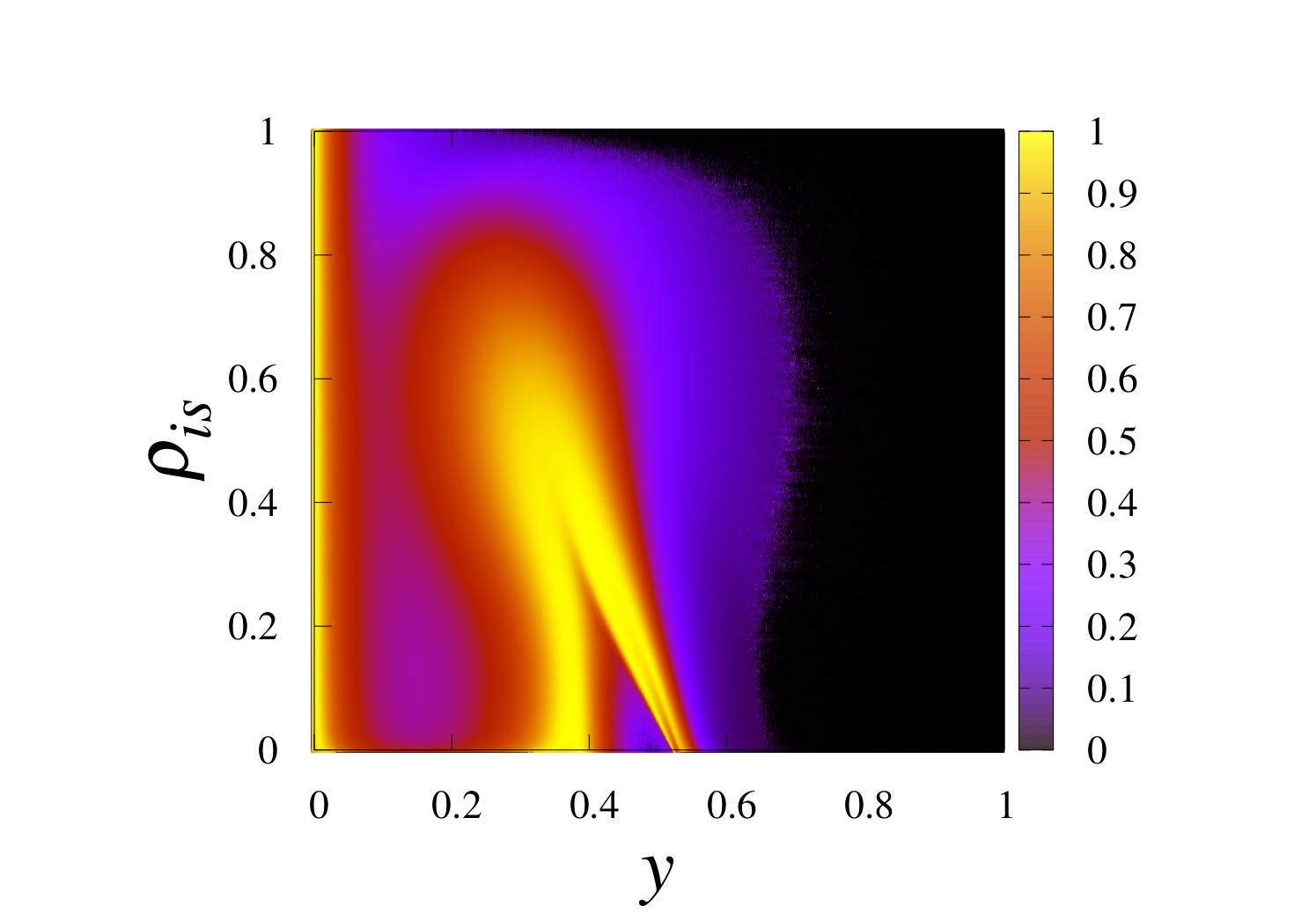
Figure 1: Color map of the coefficient of determination $r$ as function of $y$ and $rho_{is}$ for the density of vacant sites.

As can be seen, the yellow dots are points at which $r$ approaches 1 (therefore, they are candidates to phase transition points) and black dots are points at which $r$ approaches 0. In addition, we can observe that the continuous phase transition, that for the original ZGB model, is around $y=0.3874$, extends for larger values of $\rho_{is}$ and seems to be unresponsive to the density of inert sites until $\rho_{is}\simeq 0.3$. For higher values of $\rho_{is}$, the critical points move to smaller values of $y$ until $\rho_{is}\simeq 0.6$. On the other side, the discontinuous phase transition point, which for the original model is around $y\simeq 0.525$, seems to be very sensitive to $\rho_{is}$, shifting for decreasing values of $y$ as $\rho_{is}$ increases. Moreover, for small values of the density of inert sites, it is possible to observe that the two pseudocritical points of the original model fernandes2016 ; albano2001 are also present, at least for $\rho_{is}\lesssim 0.2$. Finally, this figure also shows that the two phase transitions seem to meet each other at the yellow region around $\rho_{is}\simeq 0.5$ and that there is no phase transitions when the most part of the surface is filled with inert sites or when the adsorption rate of CO molecules is above the discontinuous phase transition point of the original model. In the first case, the number of inert sites increases and the adsorption process of O₂ is hampered by the lack of nearest-neighbors available to adsorb one of the oxygen atoms. On the other hand, for higher values of $y$, the system is poisoned with CO molecules.

Figure 2 shows the color map for the density of CO molecules ($\rho_{\text{CO}}(t)$), which can also be considered as an order parameter of the model.

]

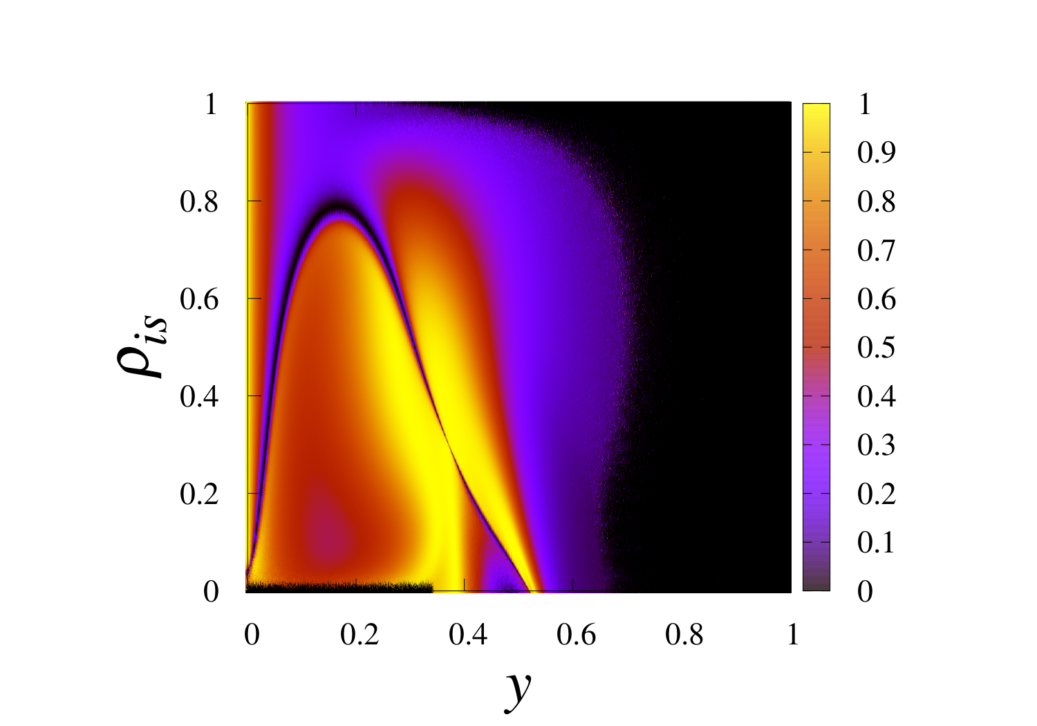
Figure 2: Color map of the coefficient of determination as function of $y$ and $\rho_{is}$ for the density of CO molecules.

Although the behavior is practically the same presented for $\rho_{\text{V}}(t)$, we are able to gather at least two more important pieces of information to those given above. The first one is that there exists a very thin line separating the points that emerged from the continuous and discontinuous phase transitions of the original model. So, we call Region 1 as the region before this thin line and that therefore comprises the continuous phase transition of the ZGB model, and Region 2 is related to the region after this line comprising the discontinuous phase transition of the original model.

The second information is that for small values of $\rho_{is}$, the Region 1 seems to have two lines with $r\simeq 1$, the first line (line 1A) starting at $y\approx 0.3$ (which arises for $\rho_{is}\neq 0$) and the second one (line 1B) starting at $y\approx 0.39$ (around the critical point of the original model). In Addition, Figs. 1 and 2 also show the existence of two lines in Region 2 with $r\simeq 1$, called lines 2A and 2B. Figure 3 shows a zoom in both regions for small values of the density of inert sites and these four curves are qualitatively represented by green straight lines.

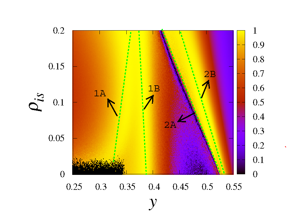
Figure 3: Color map of $r$ as function of $y$ and $\rho_{is}$ for $\rho_{\text{CO}}(t)$ and for small values of $\rho_{is}$. The green straight lines indicate, approximately, the lines of phase transition points 1A, 1B, 2A, and 2B. As can be seen, these lines are not necessarily straight.

For completeness, we also obtained the coefficient of determination for the densities of CO₂ molecules, $\rho_{\text{CO}_{2}}(t)$, and O atoms, $\rho_{\text{O}}(t)$, and their color maps are presented in Fig. 4 (a) and (b), respectively. As shown, both figures behave similarly to those presented above for $\rho_{\text{V}}(t)$ and $\rho_{\text{CO}}(t)$.

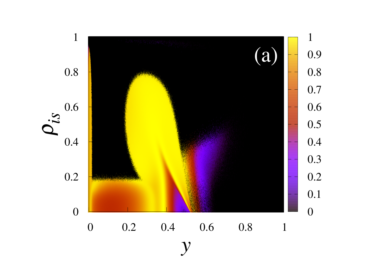
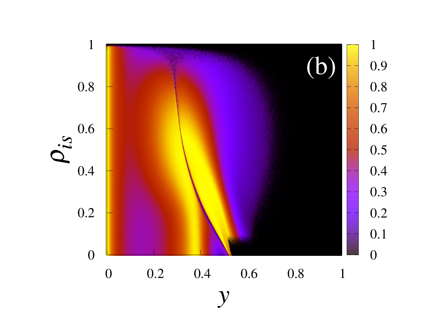
Figure 4: Color map of $r$ as function of $y$ and $\rho_{is}$ for (a) $\rho_{\text{CO}_{2}}(t)$ and (b) $\rho_{\text{O}}(t)$.

As can be seen, Figs. 2 and 4 (b) also show a region with black points for very small values of $\rho_{is}$. In Fig. 2 the black points are seen when $y\lesssim 0.35$ and in Fig. 4 (b) they appear for $y\gtrsim 0.53$. When we deal with the density of CO molecules, the black points observed in Fig. 2 refer to points where the adsorption rates are small and the system goes to an absorbing state (the available sites are filled with O atoms) at the beginning of the time evolution. Therefore, $r\simeq 0$ and there is no power law. As $\rho_{is}$ increases, the system starts to undergo phase transitions for adsorption rates smaller than that of the original model. If we look into Fig. 4 (b), we are able to see a similar behavior at the region of discontinuous phase transition, but in that case, the system is poisoned by CO molecules at the beginning of the time evolution and $r\simeq 0$ in that region.

The figures presented above show a very interesting behavior of the ZGB model when the surface possesses inert sites. The coefficient of determination was able to capture the regions of possible phase transitions when both adsorption rate and density of inert sites vary. At this point, some questions may be raised such as:

1. Are the yellow dots phase transition points?

2. Are the critical exponents varying with $y$ and $\rho_{is}$?

3. What we could state about the universality class of the model?

To answer these questions, we consider some fixed values of $\rho_{is}$ and varied the adsorption rate $y$ from 0 to 0.55. In addition, our simulations are performed for lattices of linear size $L=160$ with 20000 samples and 500 Monte Carlo steps in order to obtain both the coefficient of determination and critical points with higher precision. Next, we proceed the calculation of the critical exponents $\beta/\nu_{\parallel}$, $\theta$, $d/z$, and $1/\nu_{\parallel}$ from Eqs. (6), (7), (8), and (9), respectively. With these indexes in hand, we are able to find the static and dynamic critical exponents separately and compare them with those values found in literature. It is worth to mention that, from now on, we take into account the density of CO molecules as the order parameter of the model. Therefore, only this quantity is used to obtain our main results presented below by varying the initial conditions of the system.

To obtain the coefficient of determination and the critical adsorption rates, we carry out simulations by following two steps. In the first one, we obtain each value of $y$ (for the best value of $r$) considering $\Delta y=10^{-3}$. With these results in hand, we performed new simulations considering $\Delta y=10^{-4}$ around the former estimate. As an example, Fig. 5 shows the coefficient of determination as function of $y$ for $\rho_{is}=0.07$ for the line 1B. In the first step, we found $y_{c}=0.386$ for the higher value of $r$ and, by performing the simulations with $0.3850\leq y\leq 0.3870$ with $\Delta y=10^{-4}$, we obtained $y_{c}=0.3858$ for the critical adsorption rate when $r_{c}=0.999950$.

Figure 5: Coefficient of determination as function of $y$ for $\rho_{is}=0.07$.

This analysis was carried out for all points considered in this work and our best estimates of the coefficients of determination $r$ and the corresponding adsorption rates $y$ for several densities of inert sites $\rho_{is}$ are shown in Table 1.

Table 1: Density of inert sites $\rho_{is}$ considered in this work as well as the adsorption rates $y$ obtained for the best coefficients of determination $r$. The points are separated into two regions and four lines.

$\rho_{is}$	Region 1				Region 2
	$y_{1A}$	$r_{1A}$	$y_{1B}$	$r_{1B}$	$y_{2A}$	$r_{2A}$	$y_{1B}$	$r_{2B}$
0.00			0.3874	0.999839	0.5271	0.999498	0.5328	0.996256
0.01			0.3871	0.999862	0.5225	0.999731	0.5293	0.997592
0.02	0.3300	0.990942	0.3868	0.999886	0.5182	0.999810	0.5256	0.998490
0.03	0.3389	0.992964	0.3866	0.999898	0.5141	0.999913	0.5221	0.998955
0.04	0.3450	0.994137	0.3867	0.999915	0.5107	0.999964	0.5182	0.999376
0.05	0.3490	0.995359	0.3865	0.999922	0.5072	0.999976	0.5142	0.999591
0.06	0.3520	0.996201	0.3862	0.999941	0.5043	0.999960	0.5102	0.999766
0.07	0.3536	0.996961	0.3858	0.999950	0.5012	0.999969	0.5062	0.999858
0.08	0.3556	0.997496	0.3854	0.999950	0.4995	0.999958	0.4995	0.999958
0.09	0.3575	0.998006	0.3849	0.999958	0.4965	0.999823	0.4965	0.999823
0.10	0.3585	0.998261	0.3846	0.999963			0.4923	0.999361
0.15	0.3606	0.999289	0.3812	0.999980			0.4745	0.995093
0.20	0.3553	0.999635	0.3771	0.999993	0.4160	0.987081	0.4563	0.990847
0.25	0.3465	0.999794	0.3715	0.999985	0.3976	0.998633	0.4358	0.988602
0.30	0.3338	0.999859	0.3670	0.999910	0.3790	0.999354
0.35	0.3209	0.999874			0.3710	0.997924
0.40	0.3100	0.999859			0.3605	0.998146
0.50	0.2920	0.999695			0.3441	0.993314
0.60	0.2770	0.998240			0.3337	0.965010

This table shows, as expected, that the line 1B arises at the critical point of the original model (for $\rho_{is}=0$), where $y\simeq 0.387$, and the lines 2A and 2B also arise at the pseudocritical points which are located close to the discontinuous phase transition point of the ZGB model, $y\simeq 0.525$. However, the line 1A has a different behavior for small values of $\rho_{is}$. In fact, as presented in Fig. 3, the beginning of this line does not occur for $\rho_{is}=0$ and, therefore, can not be seen in the original model. Instead, it arises only for $\rho_{is}\neq 0$.

Table 1 also presents another important result. The adsorption rates vary according to $\rho_{is}$ for the lines 1A, 2A, and 2B, and remains stable for the line 1B (at least for small values of $\rho_{is}$), which is the line starting at the continuous phase transition point of the original model. Figure 3 also presents these points as a vertical line extending until $\rho_{is}\simeq 0.3$. This last behavior had already been predicted by Hoenicke et al. hoenicke2014 through the analysis of the behavior of moment ratios of the order parameter.

Another finding is that, the lines 2A and 2B which emerge at the two pseudocritical points of the standard ZGB model seem to meet each other in a point for $\rho_{is}\simeq 0.08$ and, from that point on, only one line probably remains. This result was presented, for the first time, by Hovi et al. in 1992 hovi1992 . They showed that, for $\rho_{is}$ greater than 8%, the first-order phase transition seemed to become continuous. Hoenicke and Figueiredo hoenicke2000 had also pointed out that a continuous phase transition emerged at $\rho_{is}=0.078$, which in turn, is also in agreement with our result. In another work, Lorenz et al. Lorenz2002 showed that the presence of inert sites on the catalytical surface had the effect of breaking up the surface into regions of different size producing, at the end, results which corroborate the appearance of a continuous phase transition even for small values of $\rho_{is}$.

In addition, once the inert fraction goes beyond $\rho_{is}\approx 0.5927$ newman2000 , the percolation threshold for square lattices, the inert sites will percolate and we are no longer able to observe any active state. Our results capture this aspect since for $\rho_{is}=0.5$ we localized a point $y_{2A}=0.3441$ with coefficient of determination $r\approx 0.993$ while for $\rho_{is}=0.6$ (after the percolation threshold) we localized a point $y_{2A}=0.3337$ with worse coefficient of determination $r\approx 0.965$. Furthermore, all values found for the coefficient of determination for $\rho_{is}\leq 0.5$ is greater than 0.99, showing that we have a sensitive decrease of $r$ when $\rho_{is}$ approaches 0.6.

After these two analyzes, we finish our study of the Region 2 and turn our attention to the Region 1, which is the region that possesses the continuous phase transition of the ZGB model (line 1B) and a line of points which emerge only for higher values of $\rho_{is}$ and around $y=0.3$. This region possesses several candidates to critical points. However, some coefficients of determination are not as close to 1 as expected for critical points, i.e., $r\simeq 1$. So, in the following analysis, we consider only points with $r\geq 0.9995$ as candidate to phase transition points. Then, we obtain the critical exponents $\beta/\nu_{\parallel}$, $\theta$, $d/z$, and $1/\nu_{\parallel}$ from Eqs. (6), (7), (8), and (9), respectively. In this study, we also consider lattices of linear size $L=160$, 20000 samples, and 500 MC steps for Eqs. (6), (7), and(8), and 1500 MC steps for Eq. (9). The error bars are obtained from 5 independent bins.

Figure 6 shows the power law decay of the density of CO molecules as function of $t$ (Eq. (6)) in $\log\times\log$ scale for four points: one point from line 1A and three points taken from line 1B.

]

Figure 6: Density of CO molecules as function of $t$ for four critical points of the model. One curve is obtained from a critical point belonging to the line 1A and three curves are taken from the line 1B. All curves present linear behavior for $t>100$ MC steps. These curves represent one bin from the five ones considered in this work.

As can be seen, after 100 MC steps, all curves follow linear behaviors meaning that, according to the short-time dynamics, these points are in fact critical points. From the slope of these curves, we are able to obtain the critical exponent $\beta/\nu_{\parallel}$.

By following this procedure for the other power law equations presented above, we calculate the corresponding critical exponents after discarding some initial MC steps. For the Eq. (6), we discarded the first 100 MC steps and for Eqs. (7) and (8) we discarded the first 200 MC steps. To obtain the linear behavior of the Eq. (9), we needed 1500 MC steps and the first 700 were discarded.

Table 2 presents all the critical exponents estimated in this work with the respective error bars.

Table 2: Static and dynamic critical exponents obtained for several critical points of the ZGB model with inert sites.

$\rho_{is}$	Region 1
	Line 1A				Line 1B
	$\beta$	$\nu_{\parallel}$	$z$	$\theta$	$\beta$	$\nu_{\parallel}$	$z$	$\theta$
0,00					0.6162(90)	1.360(17)	1.771(22)	0.223(15)
0.01					0.642(19)	1.392(37)	1.744(16)	0.224(11)
0.02					0.635(10)	1.344(20)	1.727(30)	0.213(20)
0.03					0.639(19)	1.340(36)	1.736(32)	0.198(21)
0.04					0.640(19)	1.367(37)	1.732(15)	0.2183(91)
0.05					0.633(17)	1.347(35)	1.738(41)	0.211(27)
0.06					0.642(26)	1.352(51)	1.747(36)	0.194(22)
0.07					0.655(15)	1.355(27)	1.744(20)	0.180(14)
0.08					0.661(12)	1.352(22)	1.747(23)	0.160(10)
0.09					0.668(15)	1.346(27)	1.753(34)	0.148(22)
0.10					0.682(28)	1.383(54)	1.741(34)	0.162(22)
0.15					0.748(25)	1.512(48)	1.794(26)	0.126(15)
0.20					0.733(36)	1.815(85)	1.934(68)	0.227(34)
0.25	1.664(81)	2.60(12)	6.4(1.5)	-0.971(73)	0.651(35)	2.43(13)	2.176(50)	0.383(21)
0.30	1.459(72)	3.04(15)	6.9(1.7)	-0.669(72)
0.35	1.135(31)	3.262(85)	9.1(3.3)	-0.307(47)

This table shows only three points for the line 1A which in turn present critical exponents with huge error bars. Although a power law behavior is found for Eq. (6) which lead to high values of $r$, the other equations do not follow the behavior expected for critical points (linear behavior in $\log\times\log$ scale), presenting huge fluctuations. As can be seen, the exponents $\beta$, $\nu_{\parallel}$, and $z$ have very high values, and the exponent $\theta$ is negative. So, the behavior of the functions, the huge fluctuations, and the values obtained for the exponents in this work prevented us to assert that the line 1A is a line of critical points leaving this subject as an open question which should be addressed in a future work. As the coefficient of determination is a refinement method which has proven to be very efficient in determining critical points of several models, including the ZGB model, we believe that the $r-$values obtained mainly for the three points of the line 1A presented in Table 2 are at least a clue that there is something in this region that other approaches have not been able to observe.

On the other hand, the critical exponents obtained for the line 1B are much more consistent. We can observe that the exponents for $\rho_{is}=0.00$ are very close to the values obtained for the standard ZGB model. For instance, by using both epidemic and poisoning-time analyzes, Voigt and Ziff voigt1997 obtained $\beta=0.584(4)$, $\nu_{\parallel}=1.295(6)$, $z=1.76(3)$, and $\theta=0.2295(10)$, and recently, Fernandes et al. obtained $\beta=0.586(7)$, $\nu_{\parallel}=1.292(15)$, $z=1.756(3)$, and $\theta=0.231(3)$, by means of short-time Monte Carlo simulations.

For small values of $\rho_{is}$, our results for the static critical exponent $\beta$ show a tendency of increasing and this finding is supported by the results of Hoenicke et al. hoenicke2014 . For instance, our estimates of $\beta$ for $\rho_{is}=0.01$ and $\rho_{is}=0.10$ are $\beta=0.642(19)$ and $\beta=0.682(28)$, respectively, while in Ref. hoenicke2014 , the authors found $\beta=0.623(7)$ and $\beta=0.707(7)$, respectively, which are in agreement with each other. It is interesting to observe that the static critical exponent $\nu_{\parallel}$ and the dynamic critical exponent $\theta$ seem to vary only for $\rho_{is}\geq 0.15$.

V Conclusions

In this work, we carried out nonequilibrium Monte Carlo simulations along with a refinement method in order to obtain the coefficient of determination of the ZGB model with inert sites. We presented diagrams of the possible phase transition points of the model through color maps of the coefficient of determination as function of the adsorption rates of carbon monoxide, $y$, and of the densities of inert sites, $\rho_{is}$. These diagrams showed two regions of phase transitions: one continuous and another corresponding to an extension of the discontinuous point existing for $\rho_{is}=0$. The results showed that the continuous phase transition of the original model is weakly influenced by the inclusion of inert sites on the catalytic surface. With the diagrams in hand, we turned our attention to the refinement of the phase transition points by fixing some values of density of inert sites and using larger lattices and samples in order to obtain $y$ with higher precision. Finally, we focused our attention to the region of continuous phase transitions and calculated the static critical exponents $\beta$, $\nu_{\parallel}$ and $\nu_{\perp}$ and the dynamic ones $z$ and $\theta$ for some specific points.

References

- (1) R.M. Ziff, E. Gulari, and Y. Barshad, Phys. Rev. Lett. 56, 2553 (1986).
- (2) I. Jensen and H. Fogedby, Phys. Rev. A 42, 1969 (1990).
- (3) C.H. Chan, P.A. Rikvold, Phys. Rev. E 91, 012103 (2015).
- (4) G.M. Buendía, P.A. Rikvold, Physica A. 424, 217 (2015).
- (5) J.W. Ewans, J. Chem. Phys. 98, 2463 (1993).
- (6) R. da Silva, H.A. Fernandes, Comp. Phys. Comm. 230, 1 (2018).
- (7) T. Tomé and R. Dickman, Phys. Rev. E 47, 948 (1993).
- (8) E.V. Albano, Appl. Phys. A: Mater. Sci. Proc. 55, 226 (1992).
- (9) B.J. Brosilow and R.M. Ziff, Phys. Rev. A 46, 4534 (1992).
- (10) H.P. Kaukonen and R.M. Nienimen, J. Chem. Phys. 91, 4380 (1989).
- (11) H.A. Fernandes, R. da Silva, A.B. Bernardi, Phys. Rev. E 98, 032113 (2018).
- (12) G.L. Hoenicke, M.F. de Andrade, and W. Figueiredo, J. Chem. Phys. 141, 074709 (2014).
- (13) R. da Silva, J.R. Drugowich de Felício, and A.S. Martinez, Phys. Rev. E 85, 066707 (2012).
- (14) R. da Silva, H.A. Fernandes, J. Stat. Mech.: Theor. Exp., P06011 (2015).
- (15) H.A. Fernandes, R. da Silva, E.D. Santos, P.F. Gomes, and E. Arashiro, Phys. Rev. E 94, 022129 (2016).
- (16) R. da Silva, H.A. Fernandes, J.R. Drugowich de Felício, and W. Figueiredo, Comp. Phys. Comm. 184, 2371 (2013).
- (17) R. da Silva, N. Alves Jr., and J.R. Drugowich de Felício, Phys. Rev. E 87, 012131 (2013).
- (18) R. da Silva, H.A. Fernandes, and J.R. Drugowich de Felício, Phys. Rev. E 90, 042101 (2014).
- (19) H.A. Fernandes, R. da Silva, A.A. Caparica, J.R. Drugowich de Felício, Phys. Rev. E 95, 042105 (2017).
- (20) R. da Silva, J. R. Drugowich de Felicio, H. A. Fernandes, Phys. Lett. A 383, 1235 (2019).
- (21) J.W. Evans and M.S. Miesch, Phys. Rev. Lett. 66, 833 (1991).
- (22) C.A. Voigt and R.M. Ziff, Phys. Rev. E 56, R6241 (1997).
- (23) R.M. Ziff and B.J. Brosilow, Phys. Rev. A 46, 4630 (1992).
- (24) A. Golchet, J.M. White, J. Catal. 53, 226 (1978).
- (25) T. Matsushima, H. Hashimoto, I. Toyoshima, J. Catal. 58, 303 (1979).
- (26) M. Ehsasi, M. Matloch, J.H. Block, K. Christmann, F.S. Rys, W. Hirschwald, J. Chem. Phys. 91, 4949 (1989).
- (27) K. Christmann, Introduction to Surface Physical Chemistry, Steinkopff Verlag, Darmstadt, 1991, p. 1274.
- (28) J.H. Block, M. Ehsasi, V. Gorodetskii, Prog. Surf. Sci. 42, 143 (1993).
- (29) R. Imbhil and G. Ertl, Chem. Rev. 95, 697 (1995).
- (30) J. Marro and R. Dickman, Nonequilibrium Phase Transitions in Lattice Models (Cambridge University Press, Cambridge, U.K., 1999).
- (31) B. Zheng, Int. J. Mod. Phys. B, 12, 1419 (1998), E.V. Albano, M.A. Bab, G. Baglietto, R.A. Borzi, T.S. Grigera, E.S. Loscar, D.E. Rodriguez, M.L.R. Puzzo, G.P. Saracco, Rep. Prog. Phys. 74, 026501 (2011), R. da Silva, N.A. Alves and J.R. Drugowich de Felício, Phys. Rev. E 66, 026130 (2002), R. da Silva, J.R. Drugowich de Felício, Phys. Lett. A 333, 277 (2004), H.A. Fernandes, Roberto da Silva, and J.R. Drugowich de Felício, J. Stat. Mech.: Theor. Exp., P10002 (2006).
- (32) H.K. Janssen, B. Schaub, and B. Schmittmann, Z. Phys. B: Condens. Matter 73, 539 (1989).
- (33) D.A. Huse, Phys. Rev. B 40, 304 (1989).
- (34) H. Hinrichsen, Adv. Phys. 49, 815 (2000).
- (35) R. da Silva, R. Dickman, J. R. Drugowich de Felício, Phys. Rev. E, 70, 067701 (2004).
- (36) R. da Silva, N.A. Alves, and J.R. Drugowich de Felício, Phys. Lett. A 298, 325 (2002).
- (37) P. Grassberger and Y. Zhang, Physica A 224, 169 (1996).
- (38) K.S. Trivedi, Probability and Statistics with Realiability, Queuing, and Computer Science and Applications, 2nd ed. (John Wiley and Sons, Chichester, 2002).
- (39) L. Schulke, B. Zheng, Phys. Rev. E 62, 7482 (2000).
- (40) E.V. Albano, Phys. Lett. A 288, 73 (2001).
- (41) P. de Gennes, The Physics of Liquid Crystals (Clarendon, Oxford, 1975).
- (42) L.A. Fernández, J.J. Ruiz-Lorenzo, M.P. Lombardo, A. Tarancón, Phys. Lett. B 227, 485 (1992).
- (43) J.-P. Hovi, J. Vaari, H.-P. Kaukonen, R.M. Nieminen, Comput. Mater. Sci. 1, 33 (1992).
- (44) G.L. Hoenicke and W. Figueiredo, Phys. Rev. E 62, 6216 (2000).
- (45) C.D. Lorenz, R. Haghgooie , C. Kennebrew, R.M. Ziff, Surf. Sci. 517, 75 (2002).
- (46) M.E.J. Newman and R.M. Ziff, Phys. Rev. Lett. 85, 4104 (2000).