Dual Principal Component Pursuit:
Probability Analysis and Efficient Algorithms

Abstract

Recent methods for learning a linear subspace from data corrupted by outliers are based on convex $\ell_{1}$ and nuclear norm optimization and require the dimension of the subspace and the number of outliers to be sufficiently small (Xu et al., 2010). In sharp contrast, the recently proposed Dual Principal Component Pursuit (DPCP) method (Tsakiris and Vidal, 2015) can provably handle subspaces of high dimension by solving a non-convex $\ell_{1}$ optimization problem on the sphere. However, its geometric analysis is based on quantities that are difficult to interpret and are not amenable to statistical analysis. In this paper we provide a refined geometric analysis and a new statistical analysis that show that DPCP can tolerate as many outliers as the square of the number of inliers, thus improving upon other provably correct robust PCA methods. We also propose a scalable Projected Sub-Gradient Method method (DPCP-PSGM) for solving the DPCP problem and show it admits linear convergence even though the underlying optimization problem is non-convex and non-smooth. Experiments on road plane detection from 3D point cloud data demonstrate that DPCP-PSGM can be more efficient than the traditional RANSAC algorithm, which is one of the most popular methods for such computer vision applications.

Keywords: Outliers, Robust Principal Component Analysis, High Relative Dimension, Subgradient Method, $\ell_{1}$ Minimization, Non-Convex Optimization

1 Introduction

Fitting a linear subspace to a dataset corrupted by outliers is a fundamental problem in machine learning and statistics, primarily known as (Robust) Principal Component Analysis (PCA) or Robust Subspace Recovery (Jolliffe, 1986; Candès et al., 2011; Lerman and Maunu, 2018). The classical formulation of PCA, dating back to Carl F. Gauss, is based on minimizing the sum of squares of the distances of all points in the dataset to the estimated linear subspace. Although this problem is non-convex, it admits a closed form solution given by the span of the top eigenvectors of the data covariance matrix. Nevertheless, it is well-known that the presence of outliers can severely affect the quality of the computed solution because the Euclidean norm is not robust to outliers. To clearly specify the problem, given a unit $\ell_{2}$-norm dataset $\widetilde{\mathbfcal}{X}=[\mathbfcal{X}\,\,\mathbfcal{O}]\boldsymbol{\Gamma}\in\mathbb{R}^{D\times L}$, where $\mathbfcal{X}\in\mathbb{R}^{D\times N}$ are inlier points spanning a $d$-dimensional subspace $\mathcal{S}$ of $\mathbb{R}^{D}$, $\mathbfcal{O}$ are outlier points having no linear structure, and $\boldsymbol{\Gamma}$ is an unknown permutation, the goal is to recover the inlier space $\mathcal{S}$ or equivalently to cluster the points into inliers and outliers.

1.1 Related Work

The sensitivity of classical $\ell_{2}$-based PCA to outliers has been addressed by using robust maximum likelihood covariance estimators, such as the one in (Tyler, 1987). However, the associated optimization problems are non-convex and thus difficult to provide global optimality guarantees. Another classical approach is the exhaustive-search method of Random Sampling And Consensus (RANSAC) (Fischler and Bolles, 1981), which given a time budget, computes at each iteration a $d$-dimensional subspace as the span of $d$ randomly chosen points, and outputs the subspace that agrees with the largest number of points. Even though RANSAC is currently one of the most popular methods in many computer vision applications such as multiple view geometry (Hartley and Zisserman, 2004), its performance is sensitive to the choice of a thresholding parameter. Moreover, the number of required samplings may become prohibitive in cases when the number of outliers is very large and/or the subspace dimension $d$ is large and close to the dimension $D$ of the ambient space (i.e., the high relative dimension case).

As an alternative to traditional robust subspace learning methods, during the last decade ideas from compressed sensing (Candès and Wakin, 2008) have given rise to a new class of methods that are based on convex optimization, and admit elegant theoretical analyses and efficient algorithmic implementations.

$\ell_{2,1}$-RPCA

A prominent example is based on decomposing the data matrix into low-rank (corresponding to the inliers) and column-sparse parts (corresponding to the ourliers) (Xu et al., 2010). Specifically, $\ell_{2,1}$-RPCA solves the following problem

$$\operatorname*{\text{minimize}}_{\boldsymbol{L},\boldsymbol{E}}\|\boldsymbol{L}\|_{*}+\lambda\|\boldsymbol{E}\|_{2,1},\ \operatorname*{s.t.\ }\ \boldsymbol{L}+\boldsymbol{E}=\widetilde{\mathbfcal}{X},$$ (1)

where $\|\boldsymbol{L}\|_{*}$ denotes the nulcear norm of $\boldsymbol{L}$ (a.k.a the sum of the singular values of $\boldsymbol{L}$) and $\|\boldsymbol{E}\|_{2,1}$ amounts to the sum of the $\ell_{2}$ norm of each column in $\boldsymbol{E}$. The main insight behind $\ell_{2,1}$-RPCA is that $[\mathbfcal{X}\,\,{\bf 0}]\boldsymbol{\Gamma}$ has rank $d$ which is small for a relative low dimensional subspace, while $[{\bf 0}\,\,\mathbfcal{O}]\boldsymbol{\Gamma}$ has zero columns. Since both the $\ell_{2,1}$ norm and the nuclear norm are convex functions and the later can be optimized efficiently via SemiDefinite Programming (SDP), (1) can be solved using a general SDP solver such as SDPT3 or SeDuMi. However, such methods do not scale well to large data-sets and the SDP becomes prohibitive even for modest problem sizes. As a consequence, the authors (Xu et al., 2010) proposed an efficient algorithm based on proximal gradient descent. The main limitation of this method is that it is theoretically justifiable only for subspaces of low relative dimension $d/D$ (and hence $[\mathbfcal{X}\,\,{\bf 0}]\boldsymbol{\Gamma}$ is low-rank compared to the ambient dimension $D$).

Coherence Pursuit (CoP)

Motivated by the observation that inliers lying in a low-dimensional subspace are expected to be correlated with each other while the outliers do not admit such strucuture or property, CoP (Rahmani and Atia, 2016) first measures the coherence of each point with every other point in the dataset. Compared to the outliers, the inliers tend to have higher coherence with the rest of the points in the data set. Thus, the inliers are then simply detected by selecting sufficiently number of points that have the highest coherence with the rest of the points until they span a $d$-dimensional subspace. This algorithm can be implemented very efficiently as it only involves computing the Gram matrix of the data set for the coherence and also as demonstrated in (Rahmani and Atia, 2016), CoP has a competitive performance. Similar to the $\ell_{2,1}$-RPCA, the main limitation of CoP is that it is theoretically guaranteed only for $d<\sqrt{D}$. However, for applications such as $3$D point cloud analysis, two/three-view geometry in computer vision, and system identification, a subspace of dimension $D-1$ (high relative dimension) is sought (Späth and Watson, 1987; Wang et al., 2015).

REAPER

A promising direction towards handling subspaces of high relative dimension is minimizing the sum of the distances of the points to the subspace

$$\operatorname*{\text{minimize}}_{\boldsymbol{P}_{d}}\sum_{j=1}^{L}\|({\bf I}-\boldsymbol{P}_{d})\widetilde{\boldsymbol{x}}_{j}\|_{2}\ \operatorname*{s.t.\ }\ \operatorname{trace}(\boldsymbol{P}_{d})=d,\boldsymbol{P}_{d}=\boldsymbol{P}_{d}^{\top},\text{eig}(\boldsymbol{P}_{d})=\{0,1\},$$ (2)

where $\boldsymbol{P}_{d}$ is an orthogonal projection onto any $d$-dimensinal subspace. Due to the nonconvexity of the set of orthogonal projections, (2) is a non-convex problem, which REAPER (Lerman et al., 2015a) relaxes to the following SDP:

$$\operatorname*{\text{minimize}}_{\boldsymbol{P}_{d}}\sum_{j=1}^{L}\|({\bf I}-\boldsymbol{P}_{d})\widetilde{\boldsymbol{x}}_{j}\|_{2}\ \operatorname*{s.t.\ }\ \operatorname{trace}(\boldsymbol{P}_{d})=d,\ {\bf 0}\preceq\boldsymbol{P}_{d}\preceq{\bf I}.$$ (3)

To overcome the computational issue of the above SDP solved by general SDP solvers, an Iteratively Reweighted Least Squares (IRLS) scheme is proposed in (Lerman et al., 2015a) to obtain a numerical solution of (3). Even though in practice REAPER outperforms low-rank methods (Xu et al., 2010; Soltanolkotabi et al., 2014; You et al., 2017; Rahmani and Atia, 2016) for subspaces of high relative dimension, its theoretical guarantees still require $d<(D-1)/2$.

Geodesic Gradient Descent (GGD)

The limitation mentioned above of REAPER is improved upon by the recent work of (Maunu and Lerman, 2017) that directly considers (2) by parameterizing the orthogonal projector $\boldsymbol{P}_{d}=\boldsymbol{V}\boldsymbol{V}^{\top}$ and addressing its equivalent form

$$\operatorname*{\text{minimize}}_{\boldsymbol{V}\in\mathbb{R}^{D\times d}}\sum_{j=1}^{L}\|({\bf I}-\boldsymbol{V}\boldsymbol{V}^{\top})\widetilde{\boldsymbol{x}}_{j}\|_{2}\ \operatorname*{s.t.\ }\ \boldsymbol{V}^{\mathrm{T}}\boldsymbol{V}={\bf I},$$ (4)

which is then solved by using a geodesic gradient descent (GGD) algorithm (which is a subgradient method on the Grassmannian in the strict sense). When initialized near the inlier subspace, GGD is theoretically guaranteed to converge to the inlier subspace, despite the nonconvexity of (2). In particular, with a random Gaussian model for the dataset, this convergence holds with high-probability for any $d/D$, as long as the number of outliers $M$ scales as $O(\frac{\sqrt{D(D-d)}}{d}N)$. Also as a first-order method in nature, the GGD can be implemented efficiently with each iteration mainly involving the computation of a subgradient, its singular value decompotion (SVD) and update of the subspace algong the geodesic direction. However, only a sublinear convergence rate ($O(1/\sqrt{k})$ where $k$ indicaes the total number of iteration) was formally established for GGD in (Maunu and Lerman, 2017), although a fast convergence was experimentally observed with a line search method for choosing the step sizes.

Dual Principal Component Pursuit (DPCP)

As a dual approach to (2), the recently proposed DPCP method (Tsakiris and Vidal, 2015, 2017a, 2017b) seeks to learn recursively a basis for the orthogonal complement of the subspace by solving an $\ell_{1}$ minimization problem on the sphere. In particular, the main idea of DPCP is to first compute a hyperplane $\mathcal{H}_{1}$ that contains all the inliers $\mathbfcal{X}$. Such a hyperplane can be used to discard a potentially very large number of outliers, after which a method such as RANSAC may successfully be applied to the reduced dataset . Alternatively, if $d$ is known, then one may proceed to recover $\mathcal{S}$ as the intersection of $D-d$ orthogonal hyperplanes that contain $\mathbfcal{X}$. In any case, DPCP computes a normal vector $\boldsymbol{b}_{1}$ to the first hyperplane $\mathcal{H}_{1}$ as follows:

$$\min_{\boldsymbol{b}\in\mathbb{R}^{D}}\,\|\widetilde{\mathbfcal X}^{\top}\boldsymbol{b}\|_{0}\ \operatorname*{s.t.\ }\ \boldsymbol{b}\neq 0.$$ (5)

Notice that the function $\|\widetilde{\mathbfcal X}^{\top}\boldsymbol{b}\|_{0}$ being minimized simply counts how many points in the dataset that are not contained in the hyperplane with normal vector $\boldsymbol{b}$. Assuming that there are at least $d+1$ inliers and at least $D-d$ outliers (this is to avoid degenerate situations), and that all points are in general position, then every solution $\boldsymbol{b}^{*}$ to (5) must correspond to a hyperplane that contains $\mathbfcal{X}$, and hence $\boldsymbol{b}^{*}$ is orthogonal to $\mathcal{S}$. Since (5) is computationally intractable, it is reasonable to replace it by

$$\min_{\boldsymbol{b}\in\mathbb{R}^{D}}f(\boldsymbol{b}):=\|\widetilde{\mathbfcal X}^{\top}\boldsymbol{b}\|_{1}\ \operatorname*{s.t.\ }\ \|\boldsymbol{b}\|_{2}=1.$$ (6)

In fact, the above optimization problem is equivalent to (4) for the special case $d=D-1$. As shown in (Tsakiris and Vidal, 2015, 2017a), as long as the points are well distributed in a certain deterministic sense, any global minimizer of this non-convex problem is guaranteed to be a vector orthogonal to the subspace, regardless of the outlier/inlier ratio and the subspace dimension; a result that agrees with the earlier findings of (Lerman and Zhang, 2014). Indeed, for synthetic data drawn from a hyperplane ($d=D-1$), DPCP has been shown to be the only method able to correctly recover the subspace with up to $70\%$ outliers ($D=30$). Nevertheless, the analysis of (Tsakiris and Vidal, 2015, 2017a) involves geometric quantities that are difficult to analyze in a probabilistic setting, and consequently it has been unclear how the number $M$ of outliers that can be tolerated scales as a function of the number $N$ of inliers. Moreover, even though (Tsakiris and Vidal, 2015, 2017a) show that relaxing the non-convex problem to a sequence of linear programs (LPs) guarantees finite convergence to a vector orthogonal to the subspace, this approach is computationally expensive. See Section 3.1 for the corresponding Alternating Linerization and Projection (ALP) method. Alternatively, while the IRLS scheme proposed in (Tsakiris and Vidal, 2017a, b) is more efficient than the linear programming approach, it comes with no theoretical guarantees and scales poorly for high-dimensional data, since it involves an SVD at each iteration.

We note that the literature on this subject is vast and the above mentioned related work is far from exhaustive; other methods such as the Fast Median Subspace (FMS) (Lerman and Maunu, 2017), Geometric Median Subspace (GMS) (Zhang and Lerman, 2014), Tyler M-Estimator (TME) (Zhang, 2016), Thresholding-based Outlier Robust PCA (TORP) (Cherapanamjeri et al., 2017), expressing each data point as a sparse linear combination of other data points (Soltanolkotabi et al., 2014; You et al., 2017), online subspace learning (Balzano et al., 2010), etc. For many other related methods, we refer to a recent review article (Lerman and Maunu, 2018) that thoroughly summarizes the entire body of work on robust subspace recovery.

1.2 Main Contribution and Outline

The focus of the present paper is to provide improved deterministic analysis as well as probability analysis of global optimialtiy and efficient algorithms for the DPCP approach. We make the following specific contributions.

• Theory: Although the conditions established in (Tsakiris and Vidal, 2015, 2017a) suggest that global minimizers of (6) are orthogonal to $\mathcal{S}$ (if the outliers are well distributed on the unit sphere and the inliers are well distributed on the intersection of the unit sphere with the subspace $\mathcal{S}$), they are deterministic in nature and difficult to interpret. In Section 2, we provide an improved analysis of global optimality for DPCP that replaces the cumbersome geometric quantities in (Tsakiris and Vidal, 2015, 2017a) with new quantities that are both tighter and easier to bound in probability. In order to do this, we first provide a geometric characterization of the critical points of (6) (see Lemma 12), revealing that any critical point of (6) is either orthogonal to the inlier subspace $\mathcal{S}$, or very close to $\mathcal{S}$, with its principal angle from the inlier subspace being smaller for well distributed points and smaller outlier to inlier ratios $M/N$. Employing a spherical random model, the improved global optimality condition suggests that DPCP can handle $M=O(\frac{1}{dD\log^{2}D}N^{2})$ outliers. This is in sharp contrast to existing provably correct state-of-the-art robust PCA methods, which as per the recent review (Lerman and Maunu, 2018, Table I) can tolerate at best $M=O(N)$ outliers, when the subspace dimension $d$ and the ambient dimension $D$ are fixed. The comparison of the largest number of outliers can be tolarated by different approaches is listed in Table 1, where the random models are descripted in Section 2.3.

• Algorithms: In Section 3, we first establish conditions under which solving one linear program returns a normal vector to the inlier subspace. Specifically, given an appropriate $\boldsymbol{b}_{0}$, the optimal solution of the following linear program

  $$\min_{\boldsymbol{b}\in\mathbb{R}^{D}}f(\boldsymbol{b}):=\|\widetilde{\mathbfcal X}^{\top}\boldsymbol{b}\|_{1}\ \operatorname*{s.t.\ }\ \boldsymbol{b}_{0}^{\top}\boldsymbol{b}=1$$

  must be orthogonal to the inlier subspace. This improves upon the convergence guarantee in (Tsakiris and Vidal, 2017a, b) where the ALP is only proved to converge in a finite number of iterations, but without any explict convergence rate. To further reduce the computational burden, we then provide a scalable Projected Sub-Gradient Method with piecewise geometrically diminishing step size (DPCP-PSGM), which is proven to solve the non-convex DPCP problem (6) with linear convergence and using only matrix-vector multiplications. This is in sharp contrast to classic results in the literature on PSGM methods, which usually require the problem to be convex in order to establish sub-linear convergence (Boyd et al., 2003). DPCP-PSGM is orders of magnitude faster than the ALP and IRLS schemes proposed in (Tsakiris and Vidal, 2017a), allowing us to extend the size of the datasets that we can handle from $10^{3}$ to $10^{6}$ data points.

• Experiments: Aside from experiments with synthetical data, we conduct experiments on road plane detection from 3D point cloud data using the KITTI dataset (Geiger et al., 2013), which is an important computer vision task in autonomous car driving systems. The experiments show that for the same computational budget DPCP-PSGM outperforms RANSAC, which is one of the most popular methods for such computer vision applications.

Table 1: Comparison of the largest number of outliers that can be tolarated by different approaches under a random spherical model (for the FMS, CoP and DPCP) or a random Gaussian model (for all the other approaches).

Method	random Gaussian model
GGD	$M\lesssim\frac{\sqrt{D(D-d)}}{d}N$
REAPER	$M\lesssim\frac{D}{d}N,\quad d\leq\frac{D-1}{2}$
GMS	$M\lesssim\frac{\sqrt{(D-d)D}}{d}N$
$\ell_{2,1}$-RPCA	$M\lesssim\frac{1}{d\max(1,\log(L)/d)}N$
TME	$M<\frac{D-d}{d}N$
TORP	$M\lesssim\frac{1}{d\max(1,\log(L)/d)^{2}}N$

Method	random spherical model
FMS	$N/M\gtrapprox 0$, $N\rightarrow\infty$, i.e., any ratio of outliers when$N\rightarrow\infty$
CoP	$M\lesssim\frac{D-d^{2}}{d}N,\quad d<\sqrt{D}$
DPCP	$M\lesssim\frac{1}{dD\log^{2}D}N^{2}$

1.3 Notation

We briefly introduce some of the notations used in this paper. Finite-dimensional vectors and matrices are indicated by bold characters. The symbols ${\bf I}$ and ${\bf 0}$ represent the identity matrix and zero matrix/vector, respectively. We denote the sign function by

$$\operatorname{sign}(a):=\left\{\begin{matrix}a/|a|,&a\neq 0,\\ 0,&a=0.\end{matrix}\right.$$

We also require the sub-differential $\operatorname{Sgn}$ of the absolute value function $|a|$ defined as

$$\operatorname{Sgn}(a):=\left\{\begin{matrix}a/|a|,&a\neq 0,\\ [-1,1],&a=0.\end{matrix}\right.$$ (7)

Denote by $\operatorname{sgn}(a)$ an arbitrary point in $\operatorname{Sgn}(a)$. We also use $\operatorname{sign}(\boldsymbol{a})$ to indicate that we apply the $\operatorname{sign}$ function element-wise to the vector $\boldsymbol{a}$ and similarly for $\operatorname{Sgn}$ and $\operatorname{sgn}$. The unit sphere of $\mathbb{R}^{D}$ is denoted by $\mathbb{S}^{D-1}:=\{\boldsymbol{b}\in\mathbb{R}^{D}:\|\boldsymbol{b}\|_{2}=1\}$.

2 Global Optimality Analysis for Dual Principal Component Pursuit

Although problem (6) is non-convex (because of the constraint) and non-smooth (because of the $\ell_{1}$ norm), the work of (Tsakiris and Vidal, 2015, 2017a) established conditions suggesting that if the outliers are well distributed on the unit sphere and the inliers are well distributed on the intersection of the unit sphere with the subspace $\mathcal{S}$, then global minimizers of (6) are orthogonal to $\mathcal{S}$. Nevertheless, these conditions are deterministic in nature and difficult to interpret. In this section, we give improved global optimality conditions that are i) tighter, ii) easier to interpret and iii) amenable to a probabilistic analysis.

2.1 Geometry of the Critical Points

The heart of our analysis lies in a tight geometric characterization of the critical points of (6) (see Lemma 12 below). Before stating the result, we need to introduce some further notation and definitions. Letting $\mathcal{P}_{\mathcal{S}}$ be the orthogonal projection onto $\mathcal{S}$, we define the principal angle of $\boldsymbol{b}$ from $\mathcal{S}$ as $\phi\in[0,\frac{\pi}{2}]$ such that $\cos(\phi)=\|\mathcal{P}_{\mathcal{S}}(\boldsymbol{b})\|_{2}/\|\boldsymbol{b}\|_{2}$. Since we will consider the first-order optimality condition of (6), we naturally need to compute the sub-differential of the objective function in (6). Since $f$ is convex, its sub-differental at $\boldsymbol{b}$ is defined as

$$\partial f(\boldsymbol{b}):=\left\{\boldsymbol{d}^{\prime}\in\mathbb{R}^{D}:f(\boldsymbol{a})\geq f(\boldsymbol{b})+\langle\boldsymbol{d}^{\prime},\boldsymbol{a}-\boldsymbol{b}\rangle,\ \forall\boldsymbol{a}\in\mathbb{R}^{D}\right\},$$

where each $\boldsymbol{d}^{\prime}\in\partial f(\boldsymbol{b})$ is called a subgradient of $f$ at $\boldsymbol{b}$. Note that the $\ell_{1}$ norm is subdifferetially regular. By the chain rule for subdifferentials of subdifferentially regular functions, we have

$$\partial f(\boldsymbol{b})=\widetilde{\mathbfcal}{X}\operatorname{Sgn}(\widetilde{\mathbfcal}{X}^{\top}\boldsymbol{b}).$$ (8)

Next, global minimizers of (6) are critical points in the following sense:

Definition 1

$\boldsymbol{b}\in\mathbb{S}^{D-1}$ is called a critical point of (6) if there is $\boldsymbol{d}^{\prime}\in\partial f(\boldsymbol{b})$ such that the Riemann gradient $\boldsymbol{d}=({\bf I}-\boldsymbol{b}\boldsymbol{b}^{\top})\boldsymbol{d}^{\prime}=\boldsymbol{0}$.

We now illustrate the key idea behind characterizing the geometry of the critical points. Let $\boldsymbol{b}$ be a critical point that is not orthogonal to $\mathcal{S}$. Then, under general position assumptions on the data, $\boldsymbol{b}$ can be orthogonal to $K\leq D-1$ columns of $\mathbfcal{O}$. It follows that any Riemann sub-gradient evaluated at $\boldsymbol{b}$ has the form

$$\boldsymbol{d}=({\bf I}-\boldsymbol{b}\boldsymbol{b}^{\top})\mathbfcal{X}\operatorname{sgn}(\mathbfcal{X}^{\top}\boldsymbol{b})+({\bf I}-\boldsymbol{b}\boldsymbol{b}^{\top})\mathbfcal{O}\operatorname{sign}(\mathbfcal{O}^{\top}\boldsymbol{b})+\boldsymbol{\xi},$$ (9)

where $\boldsymbol{\xi}=\sum_{i=1}^{K}\alpha_{j_{i}}\boldsymbol{o}_{j_{i}}$ with $\boldsymbol{o}_{j_{1}},\dots,\boldsymbol{o}_{j_{K}}$ the columns of $\mathbfcal{O}$ orthogonal to $\boldsymbol{b}$ and $\alpha_{j_{1}},\dots,\alpha_{j_{K}}\in[-1,1]$. Note that $\|\boldsymbol{\xi}\|_{2}<D$. Since $\boldsymbol{b}$ is a critical point, Definition 1 implies a choice of $\alpha_{j_{i}}$ so that $\boldsymbol{d}=\boldsymbol{0}$. Decompose $\boldsymbol{b}=\cos(\phi)\boldsymbol{s}+\sin(\phi)\boldsymbol{n}$, where $\phi$ is the principal angle of $\boldsymbol{b}$ from $\mathcal{S}$, and $\boldsymbol{s}=\mathcal{P}_{\mathcal{S}}(\boldsymbol{b})/\|\mathcal{P}_{\mathcal{S}}(\boldsymbol{b})\|_{2}$ and $\boldsymbol{n}=\mathcal{P}_{\mathcal{S}^{\perp}}(\boldsymbol{b})/\|\mathcal{P}_{\mathcal{S}^{\perp}}(\boldsymbol{b})\|_{2}$ are the orthonormal projections of $\boldsymbol{b}$ onto $\mathcal{S}$ and $\mathcal{S}^{\perp}$, respectively. Defining $\boldsymbol{g}=-\sin(\phi)\boldsymbol{s}+\cos(\phi)\boldsymbol{n}$ and noting that $\boldsymbol{g}\perp\boldsymbol{b}$, it follows that

$$0=\langle\boldsymbol{d},\boldsymbol{g}\rangle =\boldsymbol{g}^{\top}\mathbfcal{O}\operatorname{sign}(\mathbfcal{O}^{\top}\boldsymbol{b})+\boldsymbol{g}^{\top}\mathbfcal{X}\operatorname{sgn}(\mathbfcal{X}^{\top}\boldsymbol{b})+\boldsymbol{g}^{\top}\boldsymbol{\xi}$$

$$=\boldsymbol{g}^{\top}\mathbfcal{O}\operatorname{sign}(\mathbfcal{O}^{\top}\boldsymbol{b})-\sin(\phi)\boldsymbol{s}^{\top}\mathbfcal{X}\operatorname{sgn}(\mathbfcal{X}^{\top}\boldsymbol{s})+\boldsymbol{g}^{\top}\boldsymbol{\xi}$$

$$=\boldsymbol{g}^{\top}\mathbfcal{O}\operatorname{sign}(\mathbfcal{O}^{\top}\boldsymbol{b})-\sin(\phi)\left\|\mathbfcal{X}^{\top}\boldsymbol{s}\right\|_{1}+\boldsymbol{g}^{\top}\boldsymbol{\xi},$$

which in particular implies that

$$\sin(\phi) =\frac{\boldsymbol{g}^{\top}\mathbfcal{O}\operatorname{sign}(\mathbfcal{O}^{\top}\boldsymbol{b})+\boldsymbol{g}^{\top}\boldsymbol{\xi}}{\left\|\mathbfcal{X}^{\top}\boldsymbol{s}\right\|_{1}}$$

$$\leq\frac{\left|\boldsymbol{g}^{\top}\mathbfcal{O}\operatorname{sign}(\mathbfcal{O}^{\top}\boldsymbol{b})\right|+D}{\left\|\mathbfcal{X}^{\top}\boldsymbol{s}\right\|_{1}}$$

since $|\boldsymbol{g}^{\top}\boldsymbol{\xi}|\leq\|\boldsymbol{g}\|\|\boldsymbol{\xi}\|<D$. Thus, we obtain Lemma 12 after defining

$$\eta_{\mathbfcal{O}}:=\frac{1}{M}\max_{\boldsymbol{b}\in\mathbb{S}^{D-1}}\ \left\|({\bf I}-\boldsymbol{b}\boldsymbol{b}^{\top})\mathbfcal{O}\operatorname{sign}(\mathbfcal{O}^{\top}\boldsymbol{b})\right\|_{2}$$ (10)

and

$$c_{\mathbfcal{X},\min}:=\frac{1}{N}\min_{\boldsymbol{b}\in\mathcal{S}\cap\mathbb{S}^{D-1}}\|\mathbfcal{X}^{\top}\boldsymbol{b}\|_{1}.$$ (11)

Lemma 1

Any critical point $\boldsymbol{b}$ of (6) must either be a normal vector of $\mathcal{S}$, or have a principal angle $\phi$ from $\mathcal{S}$ smaller than or equal to $\arcsin\left(M\overline{\eta}_{\mathbfcal{O}}/Nc_{\mathbfcal{X},\min}\right)$, where

$$\overline{\eta}_{\mathbfcal{O}}:=\eta_{\mathbfcal{O}}+D/M.$$ (12)

Towards interpreting Lemma 12, we first give some insight into the quantities $\eta_{\mathbfcal{O}}$ and $c_{\mathbfcal{X},\min}$. First, we claim that $\eta_{\mathbfcal{O}}$ reflects how well distributed the outliers are, with smaller values corresponding to more uniform distributions. This can be seen by noting that as $M\rightarrow\infty$ and assuming that $\mathbfcal{O}$ remains well distributed, the quantity $\frac{1}{M}\mathbfcal{O}\operatorname{sign}\left(\mathbfcal{O}^{\top}\boldsymbol{b}\right)$ tends to the quantity $c_{D}\boldsymbol{b}$, where $c_{D}$ is the average height of the unit hemi-sphere of $\mathbb{R}^{D}$ (Tsakiris and Vidal, 2015, 2017a)

$$c_{D}:=\frac{(D-2)!!}{(D-1)!!}\cdot\left\{\begin{matrix}\frac{2}{\pi},&D\text{ is even},\\ 1,&D\text{ is old},\end{matrix}\right.\ \text{where}\ k!!:=\left\{\begin{matrix}k(k-2)(k-4)\cdots 4\cdot 2,&k\text{ is even},\\ k(k-2)(k-4)\cdots 3\cdot 1,&k\text{ is old}.\end{matrix}\right.$$ (13)

Since $\boldsymbol{g}\perp\boldsymbol{b}$, in the limit $\eta_{\mathbfcal{O}}\rightarrow 0$. Second, the quantity $c_{\mathbfcal{X},\min}$ is the same as the permeance statistic defined in (Lerman et al., 2015a), and for well-distributed inliers is bounded away from small values, since there is no single direction in $\mathcal{S}$ sufficiently orthogonal to $\mathbfcal{X}$. We thus see that according to Lemma 12, any critical point of (6) is either orthogonal to the inlier subspace $\mathcal{S}$, or very close to $\mathcal{S}$, with its principal angle $\phi$ from $\mathcal{S}$ being smaller for well distributed points and smaller outlier to inlier ratios $M/N$. Interestingly, Lemma 12 suggests that any algorithm can be utilized to find a normal vector to $\mathcal{S}$ as long as the algorithm is guaranteed to find a critical point of (6) and this critical point is sufficiently far from the subspace $\mathcal{S}$, i.e., it has principal angle larger than $\arcsin\left(M\overline{\eta}_{\mathbfcal{O}}/Nc_{\mathbfcal{X},\min}\right)$. We will utilize this crucial observation in the next section to derive guarantees for convergence to the global optimum for a new scalable algorithm.

We now compare Equation 12 with the result in (Maunu and Lerman, 2017, Theorem 1). In the case when the subspace is a hyperplane, Equation 12 and (Maunu and Lerman, 2017, Theorem 1) share similarities and differences. For comparison, we interpret the results in (Maunu and Lerman, 2017, Theorem 1) for the DPCP problem. On one hand, both Equation 12 and (Maunu and Lerman, 2017, Theorem 1) attempt to characterize certian behaviors of the objective function when $\boldsymbol{b}$ is away from the subspace by looking at the first-order information. On the other hand, we obtain Equation 12 by directly considering the Riemannian subdifferentional and proving that any Riemannian subgradient is not zero when $\boldsymbol{b}$ is away from the subspace $\mathcal{S}$ but not its normal vector. While (Maunu and Lerman, 2017, Theorem 1) is obtained by checking a particular (directional) geodesic subderivatrive and showing it is negative. These two approaches also lead to different quantities utilized for capturing the region in which there is no critical point or local minimum. Particularly, with $a{X}=\lambda_{d}\left(\sum_{i=1}^{N}\frac{\boldsymbol{x}_{i}\boldsymbol{x}_{i}^{\mathrm{T}}}{\|\boldsymbol{x}_{i}\|}\right),$ let

$$\Omega_{1}:=\left\{\boldsymbol{b}\in\mathbb{S}^{D-1}:\arcsin\left(\overline{\eta}_{\mathbfcal{O}}/c_{\mathbfcal{X},\min}\right)<\phi<\frac{\pi}{2}\right\},$$

$$\Omega_{2}:=\left\{\boldsymbol{b}\in\mathbb{S}^{D-1}:\arcsin\left(\overline{\eta}_{\mathbfcal{O}}/a_{\mathbfcal{X}}\right)<\phi<\frac{\pi}{2}\right\},$$

which are the regions in which there is no critical point and no local minimum as claimed in Equation 12 and (Maunu and Lerman, 2017, Theorem 1), respectively. We note that $c_{\mathbfcal{X},\min}$ is larger than $a_{\mathbfcal{X}}$, indicating that the region $\Omega_{1}$ is larger than $\Omega_{2}$. Also, under a probability setting, we provide a much tighter upper bound for $\overline{\eta}_{\mathbfcal{O}}$, i.e., $O(\sqrt{M})$ versus $\sqrt{M}\|\mathbfcal{O}\|_{2}$ (which roughtly scales as $O(M)$) in (Maunu and Lerman, 2017). Consequently our result leads to a much better bound on the number $M$ of outliers that can be tolerated scales as a function of the number $N$ of inliers.

We finally note that (Maunu and Lerman, 2017, Theorem 1) also covers the case where the subspace has higher co-dimension. We leave the extension of Equation 12 for multiple normal vectors as future work.

2.2 Global Optimality

In order to characterize the global solutions of (6), we define quantities similar to $c_{\mathbfcal{X},\min}$ but associated with the outliers, namely

$$c_{\mathbfcal{O},\min}:=\frac{1}{M}\min_{\boldsymbol{b}\in\mathbb{S}^{D-1}}\|\mathbfcal{O}^{\top}\boldsymbol{b}\|_{1}\ \ \text{and}\ \ c_{\mathbfcal{O},\max}:=\frac{1}{M}\max_{\boldsymbol{b}\in\mathbb{S}^{D-1}}\|\mathbfcal{O}^{\top}\boldsymbol{b}\|_{1}.$$ (14)

The next theorem, whose proof relies on Equation 12, provides new deterministic conditions under which any global solution to (6) must be a normal vector to $\mathcal{S}$.

Theorem 1

Any global solution $\boldsymbol{b}^{\star}$ to (6) must be orthogonal to the inlier subspace $\mathcal{S}$ as long as

$$\frac{M}{N}\cdot\frac{\sqrt{\overline{\eta}_{\mathbfcal{O}}^{2}+\left(c_{\mathbfcal{O},\max}-c_{\mathbfcal{O},\min}\right)^{2}}}{c_{\mathbfcal{X},\min}}<1.$$ (15)

The proof of 1 is given in Section 4.1. Towards interpreting Theorem 1, recall that for well distributed inliers and outliers $\overline{\eta}_{\mathbfcal{O}}$ is small, while the permeance statistics $c_{\mathbfcal{O},\max},\,c_{\mathbfcal{O},\min}$ are bounded away from small values. Now, the quantity $c_{\mathbfcal{O},\max}$, thought of as a dual permeance statistic, is bounded away from large values for the reason that there is not a single direction in $\mathbb{R}^{D}$ that can sufficiently capture the distribution of $\mathbfcal{O}$. In fact, as $M$ increases the two quantities $c_{\mathbfcal{O},\max},\,c_{\mathbfcal{O},\min}$ tend to each other and their difference goes to zero as $M\rightarrow\infty$. With these insights, Theorem 1 implies that regardless of the outlier/inlier ratio $M/N$, as we have more and more inliers and outliers while keeping $D$ and $M/N$ fixed, and assuming the points are well-distributed, condition (15) will eventually be satisfied and any global minimizer must be orthogonal to the inlier subspace $\mathcal{S}$.

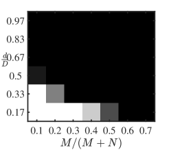
(a) Check (Tsakiris and Vidal, 2015, (24)) with $N=500$

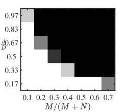
(b) Check (Tsakiris and Vidal, 2015, (24)) with $N=1000$

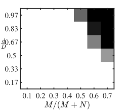
(c) Check (Tsakiris and Vidal, 2015, (24)) with $N=3000$

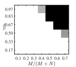
(d) Check (15) with $N=500$

(e) Check (15) with $N=1000$

(f) Check (15) with $N=3000$

Figure 1: Check whether the condition (15) and a similar condition in (Tsakiris and Vidal, 2015, Theorem 2) are satisfied (white) or not (black) for a fixed number $N$ of inliers while varying the outlier ration $M/(M+N)$ and the subspace relative dimension $d/D$. The inliers and outliers are generated in the same way as in Figure 5.

We note that a similar condition to (15) is also given in (Tsakiris and Vidal, 2015, Theorem 2). Although the proofs of the two theorems share some common elements, (Tsakiris and Vidal, 2015, Theorem 2) is derived by establishing discrepancy bounds between (6) and a continuous analogue of (6), and involves quantities difficult to handle such as spherical cap discrepancies and circumradii of zonotopes. In addition, as shown in Figure 1, a numerical comparison of the conditions of the two theorems reveals that condition (15) is much tighter. We attribute this to the quantities in our new analysis better representing the function $\|\widetilde{\mathbfcal X}^{\top}\boldsymbol{b}\|_{1}$ being minimized, namely $c_{\mathbfcal{X},\min}$, $c_{\mathbfcal{O},\min}$, $c_{\mathbfcal{O},\max}$, and $\overline{\eta}_{\mathbfcal{O}}$, when compared to the quantities used in the analysis of (Tsakiris and Vidal, 2015, 2017a). Moreover, our quantities are easier to bound under a probabilistic model, thus leading to the following characterization of the number of outliers that may be tolerated.

Theorem 2

Consider a random spherical model where the columns of $\mathbfcal{O}$ and $\mathbfcal{X}$ are drawn independently and uniformly at random from the unit sphere $\mathbb{S}^{D-1}$ and the intersection of the unit sphere with a subspace $\mathcal{S}$ of dimension $d<D$, respectively. Then for any positive scalar $t<2(c_{d}\sqrt{N}-2)$, with probability at least $1-6e^{-{t^{2}}/{2}}$, any global solution of (6) is orthogonal to $\mathcal{S}$ as long as

$$(4+t)^{2}M+C_{0}\left(\sqrt{D}\log D+t\right)^{2}M\leq\Big{(}c_{d}N-(2+{t}/{2})\sqrt{N}\Big{)}^{2},$$ (16)

where $C_{0}$ is a universal constant that is indepedent of $N,M,D,d$ and $t$, and $c_{d}$ is defined in (13).

The proof of 2 is given in Section 4.2. To interpret (16), first note that $\sqrt{\frac{2}{\pi d}}\leq c_{d}\leq\sqrt{\frac{1}{d}}$ for any $d\in\mathbb{N}$. As a consequence, (16) implies that at least $N>2\frac{1}{c_{d}^{2}}\geq 2d$. More interestingly, according to Theorem 2 DPCP can tolerate $M=O(\frac{1}{dD\log^{2}D}N^{2})$ outliers, and particularly $M=O(N^{2})$ for fixed $D$ and $d$. We note that the universal constant $C_{0}$ comes from [ (Van der Vaart, 1998), Cor. 19.35] which is utilized to bound the supreme of an empirical process related to our quantity $\eta_{\mathbfcal{O}}$. However, it is possible to get rid of this constant or obtain an explit expression of the constant by utilizing a different approach to interpret $\eta_{\mathbfcal{O}}$ in the random model. With a different approach for $\eta_{\mathbfcal{O}}$, we also believe it is possible to improve the bound with respect to $D$ for (16). In particular, we expect that an alternative bound for $\eta_{\mathbfcal{O}}$ improves the condition for the success of DPCP up to $M=O(\frac{D}{d}N^{2})$. This topic will be the subject of future work.

As corollaries of 2, the following two results further establish the global optimality condition for the random spherical model in the cases of high-dimensional subspace and large-scale data points.

Corollary 1 (high-dimensional subspace)

Consider the same random spherical model as in 2. Then for any positive scalar $t<\frac{4(c_{d}\sqrt{N}-2)^{2}}{d}$, with probability at least $1-6e^{-{td}/{2}}$, any global solution of (6) is orthogonal to $\mathcal{S}$ as long as

$$(4+\sqrt{td})^{2}M+C_{0}\left(\sqrt{D}\log D+\sqrt{td}\right)^{2}M\leq\Big{(}c_{d}N-(2+\frac{\sqrt{td}}{2})\sqrt{N}\Big{)}^{2},$$ (17)

where $C_{0}$ is a universal constant in 2.

Corollary 2 (large-scale data points)

Consider the same random spherical model as in 2. Then for any $\alpha\in(0,1)$ and positive scalar $t<\frac{4(c_{d}\sqrt{N}-2)^{2}}{N^{\alpha}}$, with probability at least $1-6e^{-{tN^{\alpha}}/{2}}$, any global solution of (6) is orthogonal to $\mathcal{S}$ as long as

$$\begin{split}(4+\sqrt{tN^{\alpha}})^{2}M+C_{0}\left(\sqrt{D}\log D+\sqrt{tN^{\alpha}}\right)^{2}M&\leq\Big{(}c_{d}N-(2+\frac{\sqrt{tN^{\alpha}}}{2})\sqrt{N}\Big{)}^{2},\end{split}$$ (18)

where $C_{0}$ is a universal constant in 2.

Unlike 2, for fixed $t$, the failure probability in 1 or 2 decreases when $d$ or $N$ increases, respectively. On the other hand, (17) gives a similar bound $M\lesssim\frac{1}{dD\log^{2}D}N^{2}$ while (18) requires $M\lesssim\frac{N^{2}}{d\max\{D\log^{2}D,N^{\alpha}\}}$, which maybe slightly stronger than $M\lesssim\frac{1}{dD\log^{2}D}N^{2}$ indicated by (16).

2.3 Comparison with Existing Results

We now compare with the existing methods that are provably tolerable to the outliers. The methods are covered by a recent review in (Lerman and Maunu, 2018, Table I), including the Geodesic Gradient Descent (GGD) (Maunu and Lerman, 2017), Fast Median Subspace (FMS) (Lerman and Maunu, 2017), REAPER (Lerman et al., 2015a), Geometric Median Subspace (GMS) (Zhang and Lerman, 2014), $\ell_{2,1}$-RPCA (Xu et al., 2010) (which is called Outlier Pursuit (OP) in (Lerman and Maunu, 2018, Table I)), Tyler M-Estimator (TME) (Zhang, 2016), Thresholding-based Outlier Robust PCA (TORP) (Cherapanamjeri et al., 2017) and the Coherence Pursuit (CoP) (Rahmani and Atia, 2016). However, we note that the comparison maynot be very fair since the results summarized in (Lerman and Maunu, 2018, Table I) are established for random Gaussian models where the columns of $\mathbfcal{O}$ and $\mathbfcal{X}$ are drawn independently and uniformly at random from the distribtuion $\mathcal{N}(\boldsymbol{0},\frac{1}{D}{\bf I})$ and $\mathcal{N}(\boldsymbol{0},\frac{1}{d}\boldsymbol{S}\boldsymbol{S}^{\mathrm{T}})$ with $\boldsymbol{S}\in\mathbb{R}^{D\times d}$ being an orthonormal basis of the inlier subspace $\mathcal{S}$. Nevertheless, these two random models are closely related since each columns of $\mathbfcal{O}$ or $\mathbfcal{X}$ in the random Gaussian model is also concentrated around the sphere $\mathbb{S}^{D-1}$, especially when $d$ is large.

That being said, we now review these results on the random Gaussian model. First, the global optimality condition in (Lerman et al., 2015a) indicates that with probability at least $1-3.5e^{-td}$, the inlier subpsace can be exactly recovered by solving the convex problem (3) (possibly with a final projection step) if

$$6\left(\frac{M}{D}+1+t\right)\leq\frac{1}{\sqrt{32\pi}}\left(\frac{N}{d}-\pi(4+2t)\right),\ d\leq(D-1)/2.$$ (19)

Compared with (19) which requires $M\lesssim\frac{D}{d}N$, (16) requires $M\lesssim\frac{1}{dD\log^{2}D}N^{2}$. On one hand, when the dimension $d$ and $D$ are fixed as constants, (16) gives a better relationship between $M$ and $N$ than (19). On the other hand, the relationship between $M$ and $D$ given in (16) is worser than the one in (19).

The work of (Maunu and Lerman, 2017) establishes and interprets a local optimality condition (which is similar to Equation 12) rather than a global one for (2). Specifically, according to (Maunu and Lerman, 2017, Theorem 5), suppose that for some absolute constant $\widetilde{C}_{1}$, and other constants $0<\theta<\frac{\pi}{2}$, $0<a<1$ and $\widetilde{C}_{0}>0$,

$$\cos(\theta)\left((1-a)\sqrt{\frac{N}{d}}-\widetilde{C}_{1}\right)^{2}>\left(\frac{M}{\sqrt{dD}}+\sqrt{\frac{M}{d}}+\sqrt{\frac{2M\widetilde{C}_{0}}{dD}}\right),\ N>\frac{\widetilde{C}_{1}^{2}}{(1-a)^{2}}d.$$ (20)

Then, with probability at least $1-2e^{-c_{1}a^{2}N}-e^{-\widetilde{C}_{0}}$ for some absolute constant $c_{1}$, the inlier subspace is the only local minimizer of (2) among all the subspaces (which is one-to-one correspondence to their orthogonal projection) that have subspace angle at most $\theta$ to the inlier subspace $\mathcal{S}$. Using this, one may establish a similar global optimality condition with the approach used in 1. Here, we instead interpret our Equation 12 in the random spherical model, implying that for any positive constants $0<\theta<\frac{\pi}{2}$, if

$$\cos(\theta)\left(c_{d}N-(2+\frac{t}{2})\sqrt{N}\right)>C_{0}\left(\sqrt{D}\log\left(\sqrt{c_{D}D}\right)+t\right)\sqrt{M},\ t<2(c_{d}\sqrt{N}-2),$$ (21)

then with probability at least $1-4e^{-{t^{2}}/{2}}$, any critical point of (6) that has principal angle from $\mathcal{S}^{\perp}$ small than $\theta$ must be orthogonal to $\mathcal{S}$. Here $C_{0}$ is a universal constant in 2. Now comparing (20) and (21), (20) requires $M\lesssim\cos(\theta)\sqrt{\frac{D}{d}}N$, while (21) needs $M\lesssim\cos^{2}(\theta)\frac{1}{dD\log^{2}D}N^{2}$. As we stated before, this difference mostly owes to a much tighter upper bound for $\overline{\eta}_{\mathbfcal{O}}$, i.e., $O(\sqrt{M})$ versus $\sqrt{M}\|\mathbfcal{O}\|_{2}$ (which roughtly scales as $O(M)$) in (Maunu and Lerman, 2017).

Finally, we summarize the exact recovery condition or global optimality condition for the existing methods that are provably tolerable to the outliers in Table 1 which imitates (Lerman and Maunu, 2018, Table I). One one hand, for fixed $d$ and $D$, Table 1 indicates that DPCP in the only method that can tolerate up to $O(N^{2})$ outliers. On the other hand, the result on DPCP has suboptimal bound with respect to $D$.

3 Efficient Algorithms for Dual Principal Component Pursuit

In this section, we first review the linear programming approach proposed in (Tsakiris and Vidal, 2015, 2017a) for solving the DPCP problem (6) and provide new convergence guarantee for this approach. We then provide a projected sub-gradient method which has guaranteed convergence performance and is scalable to the problem sizes as it only uses marix-vector multiplications in each iteration.

3.1 Alternating Linerization and Projection Method

Note that the DPCP problem (6) involves a convex objective function and a non-convex feasible region, which nevertheless is easy to project onto. This structure was exploited in (Qu et al., 2014; Tsakiris and Vidal, 2015), where in the second case the authors proposed an Alternating Linearization and Projection (ALP) method that solves a sequence of linear programs (LP) with a linearization of the non-convex constraint and then projection onto the sphere. Specifically, if we denote the constraint function associated with (6) as $g(\boldsymbol{b}):=(\boldsymbol{b}^{\top}\boldsymbol{b}-1)/2$, then the first order Tayor approximation of $g(\boldsymbol{b})$ at any $\boldsymbol{w}\in\mathbb{S}^{D-1}$ is $g(\boldsymbol{b})\approx g(\boldsymbol{w})+\boldsymbol{b}^{\top}\nabla g(\boldsymbol{w})=\boldsymbol{b}^{\top}\boldsymbol{w}$. With an initial guess of $\boldsymbol{b}_{0}$, we compute a sequence of iterates $\{\boldsymbol{b}_{k}\}_{k\geq 1}$ via the update (Tsakiris and Vidal, 2017a)

$$\boldsymbol{b}_{k}=\operatorname*{\text{arg~{}min}}_{\boldsymbol{b}\in\mathbb{R}^{d}}\|\widetilde{\mathbfcal X}^{\top}\boldsymbol{b}\|_{1},\ \operatorname*{s.t.\ }\ \boldsymbol{b}^{\top}\widehat{\boldsymbol{b}}_{k-1}=1\quad\text{and}\quad\widehat{\boldsymbol{b}}_{k}={\boldsymbol{b}_{k}}/{\|\boldsymbol{b}_{k}\|_{2}},$$ (22)

where the optimization subproblem can be written as a linear program (LP) rewritting the $\ell_{1}$ norm in an equivalent linear form with auxiliary variables. An alternatively view of the constraint $\boldsymbol{b}^{\top}\widehat{\boldsymbol{b}}_{k-1}=1$ in (22) is that it defines an affine hyperplane which excludes the original point $\boldsymbol{0}$ and has $\widehat{\boldsymbol{b}}_{k-1}$ as its normal vector.

The following result establishes conditions under which $\boldsymbol{b}_{1}$ is orthogonal to the subspace $\mathcal{S}$ and new conditions to guarantee that the sequence $\{\widehat{\boldsymbol{b}}_{k}\}_{k\geq 0}$ converges to a normal vector of $\mathcal{S}$ in a finite number of iterations.

Theorem 3

Consider the sequence $\{\widehat{\boldsymbol{b}}_{k}\}_{k\geq 0}$ generated by the recursion (22). Let $\phi_{0}$ be the principal angle of $\widehat{\boldsymbol{b}}_{0}$ from $\mathcal{S}$. Then,

1. $\boldsymbol{b}_{1}$ is orthogonal to the subspace $\mathcal{S}$ if

   $$\phi_{0}>\phi_{0}^{\natural}:=\arctan\left(\frac{Mc_{\mathbfcal{O},\max}}{Nc_{\mathbfcal{X},\min}-M\overline{\eta}_{\mathbfcal{O}}}\right);$$ (23)

2. the sequence $\{\widehat{\boldsymbol{b}}_{k}\}_{k\geq 0}$ converges to a normal vector of $\mathcal{S}$ in a finite number of iterations if

   $$\phi_{0}>\phi_{0}^{\star}:=\arccos\left(\frac{\sqrt{N^{2}c^{2}_{\mathbfcal{X},\min}-M^{2}\overline{\eta}_{\mathbfcal{O}}^{2}}-M(c_{\mathbfcal{O},\max}-c_{\mathbfcal{O},\min})}{Nc_{\mathbfcal{X},\max}}\right),$$ (24)

   where $c_{\mathbfcal{X},\max}:=\frac{1}{N}\max_{\boldsymbol{b}\in\mathcal{S}\cap\mathbb{S}^{D-1}}\|\mathbfcal{X}^{\top}\boldsymbol{b}\|_{1}$.

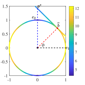
Figure 2: llustration of 3 ($i$). Here $\mathcal{S}=\operatorname{Span}(\boldsymbol{e}_{1})$, $\boldsymbol{e}_{2}$ is a normal vector and $\widehat{\boldsymbol{b}}_{0}$ is the initialization for the proceduere (22), where the minimization is equivalent to first projecting the circle onto the tangent line passing through $\widehat{\boldsymbol{b}}$ and then finding the smallest re-scaled objective value on this line.

The proof of 3 is given in Section 4.3. First note that the expressions in (23) and (24) always define angles between $0$ and $\pi/2$ when the condition (15) is satisfied. As illustrated in Figure 2, when the initialization is not very close to the subspace $\mathcal{S}$, 3 ($i$) indicates that one procedure of (22) gives a vector that is orthogonal $\mathcal{S}$, i.e., finds a hyperplance that contains all the inliers $\mathbfcal{X}$. 3 ($ii$) suggests that the requirement on the principal angle of the initialization $\widehat{\boldsymbol{b}}_{0}$ can be weakened if we are allowed to implement multiple alternating procedures in (22). To see this, for well distributed points (both inliers and outliers), the angle $\phi_{0}^{\star}$ defined in (24) tends to zero as $M,N$ go to infitiny with $M/N$ constant; while $\tan(\phi_{0}^{\natural})$ defined in (23) goes to $\Omega(M/N)$. We finally note that a similar condition to (24) is also given in (Tsakiris and Vidal, 2017a, Theorem 12). Compared with the condition in (Tsakiris and Vidal, 2017a, Theorem 12), (24) defines a slightly smaller angle $\phi_{0}^{\star}$ and again more importantly, the quantities in (15) is slightly tighter and amenable to probabilistic analysis.

3.2 Projected Sub-Gradient Method for Dual Principal Component Pursuit

Although efficient LP solvers (such as Gurobi (Gurobi Optimization, 2015)) may be used to solve each LP in the ALP approach, these methods do not scale well with the problem size (i.e., $D,N$ and $M$). Inspired by Equation 12, which states that any critical point that has principal angle larger than $\arcsin\left(M{\overline{\eta}_{\mathbfcal{O}}}/N{c_{\mathbfcal{X},\min}}\right)$ must be a normal vector of $\mathcal{S}$, we now consider solving (6) with a first-order method, specifically Projected Sub-Gradient Method (DPCP-PSGM), which is stated in Algorithm 1.

Algorithm 1 (DPCP-PSGM) Projected Sub-gradient Method for Solving (6)

Input: data $\widetilde{\mathbfcal}{X}\in\mathbb{R}^{D\times L}$ and initial step size $\mu_{0}$;
Initialization: choose $\widehat{\boldsymbol{b}}_{0}$; a typical way is to set $\widehat{\boldsymbol{b}}_{0}=\operatorname*{\text{arg~{}min}}_{\boldsymbol{b}}\|\widetilde{\mathbfcal}{X}^{\top}\boldsymbol{b}\|_{2},\ \operatorname*{s.t.\ }\ \boldsymbol{b}\in\mathbb{S}^{D-1}$;

  for $k=1,2,\ldots$ do

     1. update the step size $\mu_{k}$ according to a certain rule;

     2. perform sub-gradient method: $\boldsymbol{b}_{k}=\widehat{\boldsymbol{b}}_{k-1}-\mu_{k}\widetilde{\mathbfcal}{X}\operatorname{sign}(\widetilde{\mathbfcal}{X}^{\top}\widehat{\boldsymbol{b}}_{k-1})$;

     3. project onto the sphere $\mathbb{S}^{D-1}$: $\widehat{\boldsymbol{b}}_{k}=\mathcal{P}_{\mathbb{S}^{D-1}}\left(\boldsymbol{b}_{k}\right)=\boldsymbol{b}_{k}/\|\boldsymbol{b}_{k}\|$;

  end for

To see why it is possible that DPCP-PSGM finds a normal vector, recall that at the $k$-th step:

$$\begin{split}\boldsymbol{b}_{k}&=\widehat{\boldsymbol{b}}_{k-1}-\mu_{k}\widetilde{\mathbfcal}{X}\operatorname{sign}(\widetilde{\mathbfcal}{X}^{\top}\widehat{\boldsymbol{b}}_{k-1})\\ &=\widehat{\boldsymbol{b}}_{k-1}-\mu_{k}\mathbfcal{X}\operatorname{sign}(\mathbfcal{X}^{\top}\widehat{\boldsymbol{b}}_{k-1})-\mu_{k}\mathbfcal{O}\operatorname{sign}(\mathbfcal{O}^{\top}\widehat{\boldsymbol{b}}_{k-1}).\end{split}$$ (25)

For the rest of this section, it is more convenient to use the principal angle $\theta\in[0,\frac{\pi}{2}]$ between $\boldsymbol{b}$ and the orthogonal subspace $\mathcal{S}^{\perp}$; thus $\boldsymbol{b}$ is a normal vector of $\mathcal{S}$ if and only if $\theta=0$. Similarly let $\theta_{k}$ be the principal angle between $\widehat{\boldsymbol{b}}_{k}$ and the complement $\mathcal{S}^{\perp}$. Suppose $\theta_{k-1}>0$, i.e., $\widehat{\boldsymbol{b}}_{k-1}$ is not a normal vector to $\mathcal{S}$. We rewrite $\widehat{\boldsymbol{b}}_{k-1}$ as

$$\widehat{\boldsymbol{b}}_{k-1}=\sin(\theta_{k-1})\boldsymbol{s}_{k-1}+\cos(\theta_{k-1})\boldsymbol{n}_{k-1},$$ (26)

where $\boldsymbol{s}_{k-1}=\mathcal{P}_{\mathcal{S}}(\widehat{\boldsymbol{b}}_{k-1})/\|\mathcal{P}_{\mathcal{S}}(\widehat{\boldsymbol{b}}_{k-1})\|_{2}$ and $\boldsymbol{n}_{k-1}=\mathcal{P}_{\mathcal{S}^{\perp}}(\widehat{\boldsymbol{b}}_{k-1})/\|\mathcal{P}_{\mathcal{S}^{\perp}}(\widehat{\boldsymbol{b}}_{k-1})\|_{2}$ are the orthonormal projections of $\widehat{\boldsymbol{b}}$ onto $\mathcal{S}$ and $\mathcal{S}^{\perp}$, respectively. Since $\widehat{\boldsymbol{b}}_{k}$ is the normalized version of $\boldsymbol{b}_{k}$, they have the same principal angle to $\mathcal{S}^{\perp}$. We now consider how the principal angle changes after we apply sub-gradient method to $\widehat{\boldsymbol{b}}_{k-1}$ as in (25). Towards that end, with (26), we first decompose the term $\mathbfcal{O}\operatorname{sign}(\mathbfcal{O}^{\top}\widehat{\boldsymbol{b}}_{k-1})$ (appeared in (25)) into two parts

$$\begin{split}\mathbfcal{O}\operatorname{sign}(\mathbfcal{O}^{\top}\widehat{\boldsymbol{b}}_{k-1})&=\widehat{\boldsymbol{b}}_{k-1}\widehat{\boldsymbol{b}}_{k-1}^{\top}\mathbfcal{O}\operatorname{sign}(\mathbfcal{O}^{\top}\widehat{\boldsymbol{b}}_{k-1})+\left({\bf I}-\widehat{\boldsymbol{b}}_{k-1}\widehat{\boldsymbol{b}}_{k-1}^{\top}\right)\mathbfcal{O}\operatorname{sign}(\mathbfcal{O}^{\top}\widehat{\boldsymbol{b}}_{k-1})\\ &=\|\mathbfcal{O}^{\top}\widehat{\boldsymbol{b}}_{k-1}\|_{1}\widehat{\boldsymbol{b}}_{k-1}+\boldsymbol{q}_{k-1},\\ \end{split}$$ (27)

where we define

$$\boldsymbol{q}_{k-1}=\left({\bf I}-\widehat{\boldsymbol{b}}_{k-1}\widehat{\boldsymbol{b}}_{k-1}^{\top}\right)\mathbfcal{O}\operatorname{sign}(\mathbfcal{O}^{\top}\widehat{\boldsymbol{b}}_{k-1}),$$

which is the Riemanian subgradient of $\|\mathbfcal{O}^{\top}\boldsymbol{b}\|_{1}$ at $\boldsymbol{b}_{k-1}$. Note that $\boldsymbol{q}_{k-1}$ is expected to be small as it is bounded above by $\eta_{\mathbfcal{O}}$ (defined in (10)).

Similarly, for the other term $\mathbfcal{X}\operatorname{sign}(\mathbfcal{X}^{\top}\widehat{\boldsymbol{b}}_{k-1})$, we decompose it as

$$\begin{split}\mathbfcal{X}\operatorname{sign}(\mathbfcal{X}^{\top}\widehat{\boldsymbol{b}}_{k-1})&=\mathbfcal{X}\operatorname{sign}(\mathbfcal{X}^{\top}\boldsymbol{s}_{k-1})\\ &=\boldsymbol{s}_{k-1}\boldsymbol{s}_{k-1}^{\top}\left(\mathbfcal{X}\operatorname{sign}(\mathbfcal{X}^{\top}\boldsymbol{s}_{k-1})\right)+(\mathcal{P}_{\mathcal{S}}-\boldsymbol{s}_{k-1}\boldsymbol{s}_{k-1}^{\mathrm{T}})\left(\mathbfcal{X}\operatorname{sign}(\mathbfcal{X}^{\top}\boldsymbol{s}_{k-1})\right)\\ &=\|\mathbfcal{X}^{\top}\boldsymbol{s}_{k-1}\|_{1}\boldsymbol{s}_{k-1}+\boldsymbol{p}_{k-1},\end{split}$$ (28)

where the first equality follows because $\boldsymbol{n}_{k-1}$ is orthogonal to the inliers $\mathbfcal{X}$, and in the last equality we define

$$\boldsymbol{p}_{k-1}=\left(\mathcal{P}_{\mathcal{S}}-\boldsymbol{s}_{k-1}\boldsymbol{s}_{k-1}^{\mathrm{T}}\right)\left(\mathbfcal{X}\operatorname{sign}(\mathbfcal{X}^{\top}\boldsymbol{s}_{k-1})\right).$$

To bound $\boldsymbol{p}_{k-1}$, we also need a quantity similar to $\eta_{\mathbfcal{O}}$ that quantifies how well the inliers are distributed within the subspace $\mathcal{S}$:

$$\eta_{\mathbfcal{X}}:=\frac{1}{N}\max_{\boldsymbol{b}\in\mathcal{S}\cap\mathbb{S}^{D-1}}\left\|\left(\mathcal{P}_{\mathcal{S}}-\boldsymbol{b}\boldsymbol{b}^{\mathrm{T}}\right)\left(\mathbfcal{X}\operatorname{sign}(\mathbfcal{X}^{\top}\boldsymbol{b}\right)\right\|.$$ (29)

Similar to the disccusion for $\eta_{\mathbfcal{O}}$ after Equation 12, if we let $N\rightarrow\infty$ and assume that $\mathbfcal{X}$ remains well distributed, then the quantity $\frac{1}{N}\mathbfcal{X}\operatorname{sign}\left(\mathbfcal{X}^{\top}\boldsymbol{b}\right)$ tends to the quantity $c_{d}\boldsymbol{b}$ (where $c_{d}$ is the average height of the unit hemi-sphere of $\mathbb{R}^{d}$ defined in (13)) (Tsakiris and Vidal, 2015, 2017a). Since $\boldsymbol{g}\perp\boldsymbol{b}$, in the limit $\eta_{\mathbfcal{X}}\rightarrow 0$. By the definition of $\eta_{\mathbfcal{X}}$ in (29), we have $\frac{1}{N}\|\boldsymbol{p}_{k-1}\|\leq\eta_{\mathbfcal{X}}$.

Now plugging (27) and (28) into (25) gives

$$\begin{split}\boldsymbol{b}_{k}&=\widehat{\boldsymbol{b}}_{k-1}-\mu_{k}(\mathbfcal{X}\operatorname{sign}(\mathbfcal{X}^{\top}\widehat{\boldsymbol{b}}_{k-1})+\mathbfcal{O}\operatorname{sign}(\mathbfcal{O}^{\top}\widehat{\boldsymbol{b}}_{k-1}))\\ &=\widehat{\boldsymbol{b}}_{k-1}-\mu_{k}(\|\mathbfcal{X}^{\top}\boldsymbol{s}_{k-1}\|_{1}\boldsymbol{s}_{k-1}+\boldsymbol{p}_{k-1}+\|\mathbfcal{O}^{\top}\widehat{\boldsymbol{b}}_{k-1}\|_{1}\widehat{\boldsymbol{b}}_{k-1}+\boldsymbol{q}_{k-1})\\ &=(1-\mu_{k}\|\mathbfcal{O}^{\top}\widehat{\boldsymbol{b}}_{k-1}\|_{1})\widehat{\boldsymbol{b}}_{k-1}-\mu_{k}\|\mathbfcal{X}^{\top}\boldsymbol{s}_{k-1}\|_{1}\boldsymbol{s}_{k-1}-\mu_{k}(\boldsymbol{p}_{k-1}+\boldsymbol{q}_{k-1}).\end{split}$$ (30)

First suppose $\boldsymbol{p}_{k-1}=\boldsymbol{q}_{k-1}=\boldsymbol{0}$ and consider the simple case $\boldsymbol{b}_{k}=(1-\mu_{k}\|\mathbfcal{O}^{\top}\widehat{\boldsymbol{b}}_{k-1}\|_{1})\widehat{\boldsymbol{b}}_{k-1}-\mu_{k}\|\mathbfcal{X}^{\top}\boldsymbol{s}_{k-1}\|_{1}\boldsymbol{s}_{k-1}$. As illustrated in Figure 3, in this case, $(1-\mu_{k}\|\mathbfcal{O}^{\top}\widehat{\boldsymbol{b}}_{k-1}\|_{1})\widehat{\boldsymbol{b}}_{k-1}$ and $\mu_{k}\|\mathbfcal{X}^{\top}\boldsymbol{s}_{k-1}\|_{1}\boldsymbol{s}_{k-1}$ are the scaled version of $\widehat{\boldsymbol{b}}_{k-1}$ and $\boldsymbol{s}_{k-1}$ (which is the projection of $\widehat{\boldsymbol{b}}_{k-1}$ onto the subspace $\mathcal{S}$), respectively. Thus, as long as $\mu_{k}$ is not too large in the sense that $(1-\mu_{k}\|\mathbfcal{O}^{\top}\widehat{\boldsymbol{b}}_{k-1}\|_{1})\sin(\theta_{k-1})>\mu_{k}\|\mathbfcal{X}^{\top}\boldsymbol{s}_{k-1}\|_{1}$, the principal angle of $\boldsymbol{b}_{k}$ satisfies

$$\begin{split}\tan(\theta_{k})&=\frac{(1-\mu_{k}\|\mathbfcal{O}^{\top}\widehat{\boldsymbol{b}}_{k-1}\|_{1})\sin(\theta_{k-1})-\mu_{k}\|\mathbfcal{X}^{\top}\boldsymbol{s}_{k-1}\|_{1}}{(1-\mu_{k}\|\mathbfcal{O}^{\top}\widehat{\boldsymbol{b}}_{k-1}\|_{1})\cos(\theta_{k-1})}\\ &<\frac{(1-\mu_{k}\|\mathbfcal{O}^{\top}\widehat{\boldsymbol{b}}_{k-1}\|_{1})\sin(\theta_{k-1})}{(1-\mu_{k}\|\mathbfcal{O}^{\top}\widehat{\boldsymbol{b}}_{k-1}\|_{1})\cos(\theta_{k-1})}\\ &=\tan(\theta_{k-1}).\end{split}$$ (31)

When $\boldsymbol{p}_{k-1}$ and $\boldsymbol{q}_{k-1}$ are not zero but small, the principal angle $\theta_{k}$ is also expected to be smaller than $\theta_{k-1}$ as long as the step size $\mu_{k}$ is not too large. On the other hand, for both cases, when the step size $\mu_{k}$ is relatively large compared to $\theta_{k-1}$ in the sense that $(1-\mu_{k}\|\mathbfcal{O}^{\top}\widehat{\boldsymbol{b}}_{k-1}\|_{1})\sin(\theta_{k-1})<\mu_{k}\|\mathbfcal{X}^{\top}\boldsymbol{s}_{k-1}\|_{1}$, it is difficult (or impossible) to show the decay of the principal angle $\theta_{k}$. Instead, we will provide upper bound for the principal angle $\theta_{k}$.

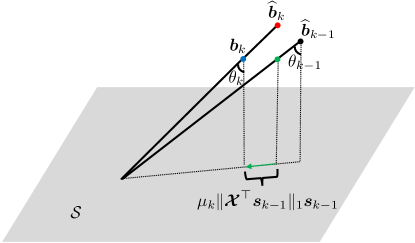
Figure 3: Illustration of (31) in the ideal case when $\boldsymbol{p}_{k-1}=\boldsymbol{0}$ and $\boldsymbol{q}_{k-1}=\boldsymbol{0}$. Here $(1-\mu_{k}\|\mathbfcal{O}^{\top}\widehat{\boldsymbol{b}}_{k-1}\|_{1})\widehat{\boldsymbol{b}}_{k-1}$ (the green dot) is the shrinkaged version of $\widehat{\boldsymbol{b}}_{k-1}$ (the black dot), while $\mu_{k}\|\mathbfcal{X}^{\top}\boldsymbol{s}_{k-1}\|_{1}\boldsymbol{s}_{k-1}$ (green line) is a scaled version $\boldsymbol{s}_{k-1}$ (which is the projection of $\widehat{\boldsymbol{b}}_{k-1}$ onto the subspace $\mathcal{S}$). As long as $\mu_{k}$ is not too large, $\boldsymbol{b}_{k}=(1-\mu_{k}\|\mathbfcal{O}^{\top}\widehat{\boldsymbol{b}}_{k-1}\|_{1})\widehat{\boldsymbol{b}}_{k-1}-\mu_{k}\|\mathbfcal{X}^{\top}\boldsymbol{s}_{k-1}\|_{1}\boldsymbol{s}_{k-1}$ (the blue dot) has smaller principal angle than $\widehat{\boldsymbol{b}}_{k-1}$ (i.e., $\theta_{k-1}<\theta_{k}$) and $\widehat{\boldsymbol{b}}_{k}$ (the red dot) is the normalized version of $\boldsymbol{b}_{k}$.

Th above analysis also reveals one fact that unlike gradient descent for smooth problems, the choice of step size for PSGM is more complicated since a constant step size in general can not guarantee the convergence of PSGM even to a critical point, though such a choice is often used in practice. For the purpose of illustration, consider a simple example $h(x)=|x|$ without any constraint, and suppose that $\mu_{k}=0.08$ for all $k$ and that an initialization of $x_{0}=0.1$ is used. Then, the iterates $\{x_{k}\}$ will jump between two points $0.02$ and $-0.06$ and never converge to the global minimum $0$. Thus, a widely adopted strategy is to use diminishing step sizes, including those that are not summable (such as $\mu_{k}=O(1/k)$ or $\mu_{k}=O(1/\sqrt{k})$) Boyd et al. (2003), or geometrically diminishing (such as $\mu_{k}=O(\rho^{k}),\rho<1$) (Goffin, 1977; Davis et al., 2018; Li et al., 2018). However, for such choices, most of the literature establishes convergence guarantees for PSGM in the context of convex feasible regions (Boyd et al., 2003; Goffin, 1977; Davis et al., 2018), and thus can not be directly applied to Algorithm 1.

Our next result provides performance guarantees for Algorithm 1 for various choices of step sizes ranging from constant to geometrically diminishing step sizes, the latter one giving an R-linear convergence of the sequence of principal angles to zero.

Theorem 4 (Convergence guarantee for PSGM)

Let $\{\widehat{\boldsymbol{b}}_{k}\}$ be the sequence generated by Algorithm 1 with initialization $\widehat{\boldsymbol{b}}_{0}$, whose principal angle $\theta_{0}$ to $\mathcal{S}^{\perp}$ is assumed to satisfy

$$\theta_{0}<\arctan\left(\frac{Nc_{\mathbfcal{X},\min}}{{N\eta_{\mathbfcal{X}}+M\eta_{\mathbfcal{O}}}}\right).$$ (32)

Also assume that

$$Nc_{\mathbfcal{X},\min}\geq N\eta_{\mathbfcal{X}}+M\eta_{\mathbfcal{O}}.$$

Let

$$\mu^{\prime}:=\frac{1}{4\cdot\max\{Nc_{\mathbfcal{X},\min},Mc_{\mathbfcal{O},\max}\}}.$$

Then the angle $\theta_{k}$ between $\widehat{\boldsymbol{b}}_{k}$ and $\mathcal{S}^{\perp}$ satisfies the following properties in accordance with various choices of step sizes.

1. (constant step size) With $\mu_{k}=\mu\leq\mu^{\prime},\ \forall k\geq 0$, we have

   $$\theta_{k}\leq\left\{\begin{matrix}\max\{\theta_{0},\theta^{\diamond}(\mu)\},&k<K^{\diamond}(\mu),\\ \theta^{\diamond}(\mu),&k\geq K^{\diamond}(\mu),\end{matrix}\right.$$ (33)

   where

   $$K^{\diamond}(\mu):=\frac{\tan(\theta_{0})}{\mu\left(Nc_{\mathbfcal{X},\min}-\max\left\{1,\tan(\theta_{0})\right\}(N\eta_{\mathbfcal{X}}+M\eta_{\mathbfcal{O}})\right)}$$ (34)

   and

   $$\theta^{\diamond}(\mu):=\arctan\left(\frac{\mu}{\sqrt{2}\mu^{\prime}}\right).$$

2. (diminishing step size) With $\mu_{k}\leq\mu^{\prime},\mu_{k}\rightarrow 0,\sum_{k=1}^{\infty}\mu_{k}=\infty$, we have $\theta_{k}\rightarrow 0$.

3. (diminishing step size of $O(1/k)$) With $\mu_{0}\leq\mu^{\prime},\mu_{k}=\frac{\mu_{0}}{k},\forall k\geq 1$, we have $\tan(\theta_{k})=O(\frac{1}{k}).$

4. (piecewise geometrically diminishing step size) With $\mu_{0}\leq\mu^{\prime}$ and

   $$\mu_{k}=\left\{\begin{matrix}\mu_{0},&k<K_{0},\\ \mu_{0}\beta^{\lfloor(k-K_{0})/K\rfloor+1},&\ k\geq K_{0},\end{matrix}\right.$$ (35)

   where $\beta<1$, $\lfloor\cdot\rfloor$ is the floor function, and $K_{0},K\in\mathbb{N}$ are chosen such that

   $$\begin{split}&K_{0}\geq K^{\diamond}(\mu_{0}),\\ &K\geq\Big{(}\sqrt{2}\beta\mu^{\prime}\Big{(}Nc_{\mathbfcal{X},\min}-(N\eta_{\mathbfcal{X}}+M\eta_{\mathbfcal{O}})\Big{)}\Big{)}^{-1},\end{split}$$ (36)

   where $K^{\diamond}(\mu)$ is defined in (34), we have

   $$\tan(\theta_{k})\leq\left\{\begin{matrix}\max\{\tan(\theta_{0}),\frac{\mu_{0}}{\sqrt{2}\mu^{\prime}}\},&k<K_{0},\\ \frac{\mu_{0}}{\sqrt{2}\mu^{\prime}}\beta^{\lfloor(k-K_{0})/K\rfloor},&k\geq K_{0}.\end{matrix}\right.$$ (37)

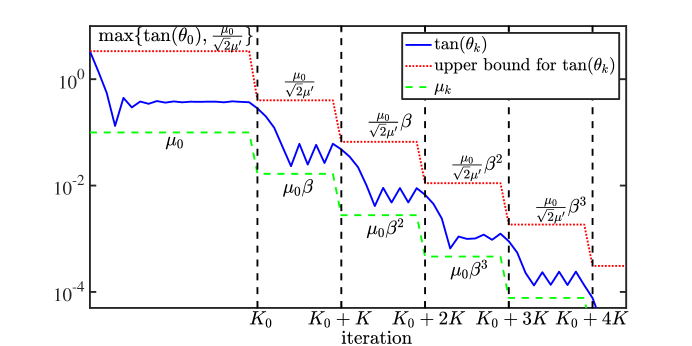
Figure 4: Illustration of 4($iv$): $\theta_{k}$ is the principal angle between $\boldsymbol{b}_{k}$ and $\mathcal{S}^{\perp}$ generated by the PSGM Algorithm 1 with piecewise geometrically diminishing step size. The red dotted line represents the upper bound on $\tan(\theta_{k})$ given by (37), while the green dashed line indicates the choice of the step size (35).

The proof of 4 is given in Section 4.4. First note that with the choice of constant step size $\mu$, although PSGM is not guaranteed to find a normal vector, (33) ensures that after $K^{\diamond}(\mu)$ iterations, $\widehat{\boldsymbol{b}}_{k}$ is close to $\mathcal{S}^{\perp}$ in the sense that $\theta_{k}\leq\theta^{\diamond}(\mu)$, which can be much smaller than $\theta_{0}$ for a sufficiently small $\mu$. The expressions for $K^{\diamond}(\mu)$ and $\theta^{\diamond}(\mu)$ indicate that there is a tradeoff in selecting the step size $\mu$. By choosing a larger step size $\mu$, we have a smaller $K^{\diamond}(\mu)$ but a larger upper bound $\theta^{\diamond}(\mu)$. We can balance this tradeoff according to the requirements of specific applications. For example, in applications where the accuracy of $\theta$ (to zero) is not as important as the convergence speed, it is appropriate to choose a larger step size. An alternative and more efficient way to balance this tradeoff is to change the step sizes as the iterations proceed. For the classical diminishing step sizes that are not summable, 4($ii$) guarantees convergence of $\theta_{k}$ to zero (i.e., the iterates converge to a normal vector), though the convergence rate depends on the specific choice of step sizes. For example, 4($iii$) guarantees a sub-linear convergence of $\tan(\theta_{k})$ for step sizes diminishing as $1/k$.

The approach of piecewise geometrically diminishing step size (see 4($iv$)) takes advantage of the tradeoff in 4($i$) by first using a relatively large initial step size $\mu_{0}$ so that $K^{\diamond}(\mu_{0})$ is small (although $\theta^{\diamond}(\mu_{0})$ is large), and then decreasing the step size in a piecewise fashion. As illustrated in Figure 4, with such a piecewise geometrically diminishing step size, (37) establishes a piecewise geometrically decaying bound for the principal angles. Note that the curve $\tan(\theta_{k})$ is not monotone because, as noted earlier, PSGM is not a descent method. Perhaps the most surprising aspect in 4($iv$) is that with the diminishing step size (35), we obtain a $K$-step $R$-linear convergence rate for $\tan(\theta_{k})$. This linear convergence rate relies on both the choice of the step size and certain beneficial geometric structure in the problem. As characterized by Equation 12, one such structure is that all critical points in a neighborhood of $\mathcal{S}^{\perp}$ are global solutions. Aside from this, other properties (e.g., the negative direction of the Riemannian subgradient points toward $\mathcal{S}^{\perp}$) are used to show the decaying rate of the principal angle. This is different from the recent work (Davis et al., 2018) in which linear convergence for PSGM is obtained for sharp and weakly convex objective functions and convex constraint sets. Very recently, for the same optimization problem (6) in the context of orthonormal dictionary learning, Bai et al. (2018) also utilized a subgradient method but with step size $\mu_{k}=O(1/k^{3/8})$, giving a sublinear convergence which is slower than the piecewise linear convergence. Thus, we believe the choice of piecewise geometrically diminishing step size is of independent interest and can be useful for other nonsmooth problems.

3.3 Initialization

Random Initialization

We first consider $\widehat{\boldsymbol{b}}_{0}$ drawn randomly from the unit sphere $\mathbb{S}^{D-1}$. For such initialization, we analyze its principal angle to $\mathcal{S}^{\perp}$ in expectation.

Lemma 2

Let $\widehat{\boldsymbol{b}}_{0}$ be drawn randomly from the unit sphere $\mathbb{S}^{D-1}$. Then

$$\sqrt{\frac{d-1/2}{D}}\leq\operatorname{\mathbb{E}}[\sin(\theta_{0})]=\frac{B(\frac{d}{2}+\frac{1}{2},\frac{D-d}{2})}{B(\frac{d}{2},\frac{D-d}{2})}\leq\sqrt{\frac{d}{D-1/2}},$$

where $\theta_{0}$ is the principal angle of $\widehat{\boldsymbol{b}}_{0}$ from $\mathcal{S}^{\perp}$ and $B(\cdot,\cdot)$ is the beta function.

The proof of 2 is given in Section 4.5.1. 2 generalizes the result in (Goldstein and Studer, 2018, Lemma 5) which analyzes the inner product between two random vectors on the unit sphere. 2 indicates that when the subspace dimension $d$ is small, then in expectation a random initialization has a small principal angle from $\mathcal{S}^{\perp}$. However, if $d$ is large (say $d=D-1$), then it is very possible that a random vector is very close to $\mathcal{S}$, irrespectively of the data matrix. This is because generating a random vector does not utilize the data matrix $\widetilde{\mathbfcal}{X}$, although it is among the easiest ones for initialization. Thus, it is possible to obtain a better initialization from more sophisticated methods using $\widetilde{\mathbfcal}{X}$.

Spectral Initialization

Another commonly used strategy is to use a spectral method generating an initialization which has much better guaranteed performance than a random one  (Lu and Li, 2017). For our problem, we use the smallest eigenvector of $\widetilde{\mathbfcal}{X}\widetilde{\mathbfcal}{X}^{\mathrm{T}}$, i.e., the classical PCA approach for finding a normal vector from the data $\widetilde{\mathbfcal}{X}$.

Lemma 3

Consider a spectral initialization $\widehat{\boldsymbol{b}}_{0}$ by taking the bottom eigenvector of $\widetilde{\mathbfcal}{X}\widetilde{\mathbfcal}{X}^{\mathrm{T}}$. Then, $\theta_{0}$ (the principal angle of $\widehat{\boldsymbol{b}}_{0}$ from $\mathcal{S}^{\perp}$) satisfies

$$\sin(\theta_{0})<\sqrt{\sigma_{1}^{2}(\mathbfcal{O})-\sigma_{D}^{2}(\mathbfcal{O})}/{\sigma_{d}(\mathbfcal{X})},$$ (38)

where $\sigma_{\ell}$ denotes the $\ell$-th largest singular value.

The proof of 3 is given in Section 4.5.2. This result together with 4 gives a formally guarantee of the PSGM with a spectral initialization $\boldsymbol{b}_{0}$.

Corollary 3

Suppose the inliers and outliers satisfy

$$\begin{split}\frac{\sigma_{1}^{2}(\mathbfcal{O})-\sigma_{D}^{2}(\mathbfcal{O})}{\sigma_{d}^{2}(\mathbfcal{X})-\left(\sigma_{1}^{2}(\mathbfcal{O})-\sigma_{D}^{2}(\mathbfcal{O})\right)}&<\left(\frac{Nc_{\mathbfcal{X},\min}}{{N\eta_{\mathbfcal{X}}+M\eta_{\mathbfcal{O}}}}\right)^{2},\\ Nc_{\mathbfcal{X},\min}&\geq N\eta_{\mathbfcal{X}}+M\eta_{\mathbfcal{O}}.\end{split}$$ (39)

Then, the PSGM (see Algorithm 1) with a spectral initialization $\widehat{\boldsymbol{b}}_{0}$ (i.e., the bottom eigenvector of $\widetilde{\mathbfcal}{X}\widetilde{\mathbfcal}{X}^{\mathrm{T}}$) and piecewise geometricallly deminishing stepsizes as in 4 converges to a normal vector in a linear convergence rate.

3 follows directly by letting the upper bound of $\theta_{0}$ specified in (38) satisfy the requirement in (32). We now interpret the above results in a random spherical model as used in 2.

Corollary 4

Consider the same random spherical model as in 2. Then for any positive number $t<\min\{\sqrt{N}-C_{2}\sqrt{d},2c_{d}\sqrt{N}-4\}$, with probability at least $1-3e^{-{t^{2}}/{2}}-3e^{-C_{1}t^{2}}$, the PSGM with a spectral initialization $\widehat{\boldsymbol{b}}_{0}$ and piecewise geometricallly deminishing stepsizes converges to a normal vector in a linear convergence rate provided that

$$\begin{split}\frac{\frac{\sqrt{D}}{d}\left(\sqrt{N}-C_{2}\sqrt{d}-t\right)^{2}}{4C_{2}\sqrt{M}+4C_{2}t}&>1+\left(\frac{C_{0}\left(\sqrt{d}\log d\sqrt{N}+\sqrt{D}\log D\sqrt{M}+t(\sqrt{N}+\sqrt{M})\right)}{c_{d}N-(2+\frac{t}{2})\sqrt{N}}\right)^{2},\\ \Big{(}c_{d}N-(2+{t}/{2})\sqrt{N}\Big{)}&\geq C_{0}\left(\left(\sqrt{D}\log D+t\right)\sqrt{M}+\left(\sqrt{d}\log d+t\right)\sqrt{N}\right),\end{split}$$ (40)

where $c_{d}$ and $c_{D}$ are defined in (13), and $C_{0},C_{1}$ and $C_{2}$ are universal constants indepedent of $N,M,D,d$ and $t$.

The proof of 4 is given in Section 4.5.3. Note that when $\mathbfcal{O}$ is a Gaussian random matrix whose entries are independent normal random variables of mean $0$ and variance $\frac{1}{D}$, $C_{1}=C_{2}=1$. Thus we suspect that $C_{1}$ and $C_{2}$ are also close to $1$ in 4. Note that the LHS of the first line in (40) is $O(\frac{N\sqrt{D}}{\sqrt{M}d})$, while the RHS of the first line is $1+O(\frac{dD\log^{2}DM}{N^{2}}+\frac{d^{2}\log^{2}d}{N})$. This together with the second line suggests that (40) is satisfied when $M\lesssim\frac{1}{dD\log^{2}D}N^{2}$ and $N\gtrsim d^{2}\log^{2}d$, implying that the DPCP-PSGM with a spectral initialization can tolerate $M=O(\frac{1}{dD\log^{2}D}N^{2})$ outliers, matching the bound given in 2.

4 Proofs

4.1 Proof of 1

Let $\boldsymbol{b}^{\star}$ be an optimal solution of (6). For the sake of contradiction, suppose that $\boldsymbol{b}^{\star}\not\perp\mathcal{S}$, i.e., its principal angle $\phi^{\star}$ to the subspace $\mathcal{S}$ satisfies $\phi^{\star}<\frac{\pi}{2}$. It then follows from Equation 12 that

$$\sin(\phi^{\star})\leq\frac{M\overline{\eta}_{\mathbfcal{O}}}{Nc_{\mathbfcal{X},\min}}.$$

On the other hand, utilizing the fact that $\boldsymbol{b}^{\star}$ is a global minimum, we have

$$\cos(\phi^{\star})Nc_{\mathbfcal{X},\min}+Mc_{\mathbfcal{O},\min}\leq g(\boldsymbol{b}^{\star})\leq\min_{\boldsymbol{b}\in\mathbb{S}^{D-1},\boldsymbol{b}\perp\mathcal{S}}\|\widetilde{\mathbfcal}{X}^{\top}\boldsymbol{b}\|_{1}=\min_{\boldsymbol{b}\in\mathbb{S}^{D-1},\boldsymbol{b}\perp\mathcal{S}}\|\mathbfcal{O}^{\top}\boldsymbol{b}\|_{1}\leq Mc_{\mathbfcal{O},\max},$$

which gives

$$\cos(\phi^{\star})\leq\frac{M(c_{\mathbfcal{O},\max}-c_{\mathbfcal{O},\min})}{Nc_{\mathbfcal{X},\min}}.$$

Combining the above inequalities on $\phi^{\star}$ yields

$$1=\sin^{2}(\phi^{\star})+\cos^{2}(\phi^{\star})\leq\frac{M^{2}(\overline{\eta}_{\mathbfcal{O}}^{2}+\left(c_{\mathbfcal{O},\max}-c_{\mathbfcal{O},\min}\right)^{2})}{N^{2}c^{2}_{\mathbfcal{X},\min}}.$$

But this contradicts to (15).

4.2 Proof of Theorem 2

The proof of 2 follows directly from 1 and the following results concerning different quantities in a random spherical model.

Lemma 4

Consider a random spherical model where the columns of $\mathbfcal{O}$ and $\mathbfcal{X}$ are drawn independently and uniformly at random from the unit sphere $\mathbb{S}^{D-1}$ and the intersection of the unit sphere and a subspace $\mathcal{S}$ of dimension $d<D$, respectively. Fix a number $t>0$. Then

$$\operatorname{\mathbb{P}}\left[c_{\mathbfcal{O},\min}\geq c_{D}-(2+\frac{t}{2})/\sqrt{M}\right]\geq 1-2e^{-\frac{t^{2}}{2}},$$

$$\operatorname{\mathbb{P}}\left[c_{\mathbfcal{O},\max}\leq c_{D}+(2+\frac{t}{2})/\sqrt{M}\right]\geq 1-2e^{-\frac{t^{2}}{2}},$$

$$\operatorname{\mathbb{P}}\left[\eta_{\mathbfcal{O}}\lesssim\left(\sqrt{D}\log\left(\sqrt{c_{D}D}\right)+t\right)/\sqrt{M}\right]\geq 1-2e^{-\frac{t^{2}}{2}}$$

$$\operatorname{\mathbb{P}}\left[c_{\mathbfcal{X},\min}\geq c_{d}-(2+\frac{t}{2})/\sqrt{N}\right],\geq 1-2e^{-\frac{t^{2}}{2}},$$

where $\frac{1}{D}<c_{D}\approx\sqrt{\frac{2}{\pi D}}<1$ is defined in (13).

The proof of 4 is given in Section A. We note that the above results are not optimized and thus it is possible to have much tighter results by more sophisticated analysis or a different random model. For example, for a random Gaussian model, a slightly tighter bound for $c_{\mathbfcal{O},\min}$ is given in (Lerman et al., 2015b) as follows:

$$\operatorname{\mathbb{P}}\left[c_{\mathbfcal{O},\min}\geq\frac{2}{\pi\sqrt{D}}-2\sqrt{\frac{1}{M}}-t\frac{1}{\sqrt{MD}}\right]\geq 1-e^{-\frac{t^{2}}{2}}.$$ (41)

4.3 Proof of 3

We individually prove the two arguments in 3.

Proof of part $(i)$:

We first rewrite the initialization $\widehat{\boldsymbol{b}}_{0}$ by $\widehat{\boldsymbol{b}}_{0}=\cos(\phi_{0})\boldsymbol{s}_{0}+\sin(\phi_{0})\boldsymbol{n}_{0}$, where $\phi_{0}$ is the principal angle of $\widehat{\boldsymbol{b}}_{0}$ from $\mathcal{S}$, and $\boldsymbol{s}_{0}=\mathcal{P}_{\mathcal{S}}(\widehat{\boldsymbol{b}}_{0})/\|\mathcal{P}_{\mathcal{S}}(\widehat{\boldsymbol{b}}_{0})\|_{2}$ and $\boldsymbol{n}=\mathcal{P}_{\mathcal{S}^{\perp}}(\widehat{\boldsymbol{b}}_{0})/\|\mathcal{P}_{\mathcal{S}^{\perp}}(\widehat{\boldsymbol{b}}_{0})\|_{2}$ are the orthonormal projections of $\widehat{\boldsymbol{b}}_{0}$ onto $\mathcal{S}$ and $\mathcal{S}^{\perp}$, respectively. For any variable $\boldsymbol{b}$ in (22) that is not required on the unit sphere , we similarly decompose it by $\boldsymbol{b}=\alpha\boldsymbol{s}+\beta\boldsymbol{n}$, where $\alpha=\|\mathcal{P}_{\mathcal{S}}(\boldsymbol{b})\|_{2}$, $\boldsymbol{s}=\mathcal{P}_{\mathcal{S}}(\boldsymbol{b})/\alpha$, $\beta=\|\mathcal{P}_{\mathcal{S}^{\perp}}(\boldsymbol{b})\|_{2}$, $\boldsymbol{n}=\mathcal{P}_{\mathcal{S}^{\perp}}(\boldsymbol{b})/\beta$, and $\alpha\boldsymbol{s}$ and $\beta\boldsymbol{n}$ are the orthonormal projections of $\boldsymbol{b}$ onto $\mathcal{S}$ and $\mathcal{S}^{\perp}$, respectively. Now we rewrite the the $\ell_{1}$ minimization in (22) as

$$\begin{split}&\min_{\alpha,\beta,\boldsymbol{s},\boldsymbol{n}}f_{1}(\alpha,\beta,\boldsymbol{s},\boldsymbol{n}):=\|\widetilde{\mathbfcal X}^{\mathrm{T}}(\alpha\boldsymbol{s}+\beta\boldsymbol{n})\|_{1},\\ &\operatorname*{s.t.\ }\ \alpha\cos(\phi_{0})\boldsymbol{s}^{\top}\boldsymbol{s}_{0}+\beta\sin(\phi_{0})\boldsymbol{n}^{\top}\boldsymbol{n}_{0}=1.\end{split}$$ (42)

Recall that the objective function consisits of two parts corresponding to inliers and outliers:

$$\|\widetilde{\mathbfcal X}^{\mathrm{T}}(\alpha\boldsymbol{s}+\beta\boldsymbol{n})\|_{1}=\|{\mathbfcal X}^{\top}\alpha\boldsymbol{s}\|_{1}+\|{\mathbfcal O}^{\mathrm{T}}(\alpha\boldsymbol{s}+\beta\boldsymbol{n})\|_{1}.$$ (43)

To show that (42) achieves its global minimum only at $\alpha=0$ (i.e., $\boldsymbol{b}$ is a normal vector of $\mathcal{S}$), we first separate $\alpha$ and $\beta$ in $\|{\mathbfcal O}^{\mathrm{T}}(\alpha\boldsymbol{s}+\beta\boldsymbol{n})\|_{1}$ with a surrogate function which is not greater than $\|{\mathbfcal O}^{\mathrm{T}}(\alpha\boldsymbol{s}+\beta\boldsymbol{n})\|_{1}$. Specifically, we have

$$\|{\mathbfcal O}^{\mathrm{T}}(\alpha\boldsymbol{s}+\beta\boldsymbol{n})\|_{1}\geq\beta\|{\mathbfcal O}^{\top}\boldsymbol{n}\|_{1}-\alpha M\overline{\eta}_{\mathbfcal{O}},$$ (44)

where $\overline{\eta}_{\mathbfcal{O}}$ is defined in (12). Before proving (44), we note that by the triangle inequality of the norm, an alternative version of (44) is

$$\|{\mathbfcal O}^{\mathrm{T}}(\alpha\boldsymbol{s}+\beta\boldsymbol{n})\|_{1}\geq\beta\|{\mathbfcal O}^{\top}\boldsymbol{n}\|_{1}-\alpha\|\mathbfcal{O}^{\top}\boldsymbol{s}\|_{1}.$$ (45)

However, the bound in (45) is too loose in that when we plug (45) into (43), we arrive at $\|\widetilde{\mathbfcal X}^{\mathrm{T}}(\alpha\boldsymbol{s}+\beta\boldsymbol{n})\|_{1}\geq\alpha(\|{\mathbfcal X}^{\top}\boldsymbol{s}\|_{1}-\|{\mathbfcal O}^{\top}\boldsymbol{s}\|_{1})+\|{\mathbfcal O}^{\mathrm{T}}(\alpha\boldsymbol{s}+\beta\boldsymbol{n})\|_{1}$, which is useful only when $\|{\mathbfcal X}^{\top}\boldsymbol{s}\|_{1}-\|{\mathbfcal O}^{\top}\boldsymbol{s}\|_{1}>0$ (which requires the number of outliers $M\lesssim N$).

On the other hand, intuitively, as $M\rightarrow\infty$ and assuming that $\mathbfcal{O}$ remains well distributed, the quantity $\frac{1}{M}\|{\mathbfcal O}^{\mathrm{T}}(\alpha\boldsymbol{s}+\beta\boldsymbol{n})\|_{1}\rightarrow c_{D}\sqrt{\alpha^{2}+\beta^{2}}$ and $\frac{1}{M}\beta\|{\mathbfcal O}^{\top}\boldsymbol{n}\|_{1}\rightarrow c_{D}\beta$, which suggests that $\|{\mathbfcal O}^{\mathrm{T}}(\alpha\boldsymbol{s}+\beta\boldsymbol{n})\|_{1}\geq\beta\|{\mathbfcal O}^{\top}\|_{1}$ is expected. We now turn to prove (44). To that end, define

$$\chi(\alpha)=\|{\mathbfcal O}^{\mathrm{T}}(\alpha\boldsymbol{s}+\beta\boldsymbol{n})\|_{1}-\beta\|{\mathbfcal O}^{\top}\boldsymbol{n}\|_{1}+\alpha M\overline{\eta}_{\mathbfcal{O}}.$$ (46)

In what follows, we show $\chi(\alpha)$ is an increasing function since together with the fact $\chi(0)=0$, it is a sufficient condition for (44). Towards that end, we let $\widehat{\boldsymbol{b}}=\cos(\phi)\boldsymbol{s}+\sin(\phi)\boldsymbol{n}$ (where $\phi=\arccos\left(\frac{\alpha}{\sqrt{\alpha^{2}+\beta^{2}}}\right)$) be the projection of $\boldsymbol{b}$ onto the sphere $\mathbb{S}^{D-1}$ and compute the subdifferential of $\chi(\alpha)$ as

$$\partial\chi(\alpha)=\sum_{i=1}^{M}\operatorname{Sgn}(\boldsymbol{o}_{i}^{\top}(\alpha\boldsymbol{s}+\beta\boldsymbol{n}))\boldsymbol{o}_{i}^{\top}\boldsymbol{s}+M\overline{\eta}_{\mathbfcal{O}}=\sum_{i=1}^{M}\operatorname{Sgn}(\boldsymbol{o}_{i}^{\top}\widehat{\boldsymbol{b}})\boldsymbol{o}_{i}^{\top}\boldsymbol{s}+M\overline{\eta}_{\mathbfcal{O}}.$$ (47)

Now for any $a\in\partial\chi(\alpha)$, we can write it as $a=\sum_{i=1}^{M}\operatorname{sgn}(\boldsymbol{o}_{i}^{\top}\widehat{\boldsymbol{b}})\boldsymbol{o}_{i}^{\top}\boldsymbol{s}+M\overline{\eta}_{\mathbfcal{O}}$. It follows that

$$a=\sum_{i=1}^{M}\operatorname{sgn}(\boldsymbol{o}_{i}^{\top}\widehat{\boldsymbol{b}})\boldsymbol{o}_{i}^{\top}\boldsymbol{s}+M\overline{\eta}_{\mathbfcal{O}}$$

$$=\sum_{i=1}^{M}\operatorname{sgn}(\boldsymbol{o}_{i}^{\top}\widehat{\boldsymbol{b}})\boldsymbol{o}_{i}^{\top}\left(\cos(\theta)(\cos(\theta)\boldsymbol{s}+\sin(\theta)\boldsymbol{n})-\sin(\theta)(-\sin(\theta)\boldsymbol{s}+\cos(\theta)\boldsymbol{n})\right)+M\overline{\eta}_{\mathbfcal{O}}$$

$$=\cos(\theta)\|\mathbfcal{O}^{\top}\widehat{\boldsymbol{b}}\|_{1}-\sin(\theta)\sum_{i=1}^{M}\operatorname{sgn}(\boldsymbol{o}_{i}^{\top}\widehat{\boldsymbol{b}})\boldsymbol{o}_{i}^{\top}\boldsymbol{\xi}_{\widehat{\boldsymbol{b}}}+M\overline{\eta}_{\mathbfcal{O}}$$

$$\geq-\sum_{i=1}^{M}\operatorname{sgn}(\boldsymbol{o}_{i}^{\top}\widehat{\boldsymbol{b}})\boldsymbol{o}_{i}^{\top}\boldsymbol{\xi}_{\widehat{\boldsymbol{b}}}+M\overline{\eta}_{\mathbfcal{O}}$$

where $\boldsymbol{\xi}_{\widehat{\boldsymbol{b}}}=(-\sin(\theta)\boldsymbol{s}+\cos(\theta)\boldsymbol{n})$. By rewriting $\operatorname{sgn}$ with $\operatorname{sign}$ as in (9) and using the general assumption of outliers, we have

$$\sum_{i=1}^{M}\left|\operatorname{sgn}(\boldsymbol{o}_{i}^{\top}\widehat{\boldsymbol{b}})\boldsymbol{o}_{i}^{\top}\boldsymbol{\xi}_{\widehat{\boldsymbol{b}}}\right|\leq M\overline{\eta}_{\mathbfcal{O}},$$

Thus, we have $a\geq 0$ for any $a\in\partial\chi(\alpha)$ and therefore (44) follows.

Now plugging (44) into (43), we have

$$\|\widetilde{\mathbfcal X}^{\mathrm{T}}(\alpha\boldsymbol{s}+\beta\boldsymbol{n})\|_{1} =\|{\mathbfcal X}^{\top}\alpha\boldsymbol{s}\|_{1}+\|{\mathbfcal O}^{\mathrm{T}}(\alpha\boldsymbol{s}+\beta\boldsymbol{n})\|_{1}\geq\alpha\|{\mathbfcal X}^{\top}\boldsymbol{s}\|_{1}+\beta\|{\mathbfcal O}^{\top}\boldsymbol{n}\|_{1}-\alpha M\overline{\eta}_{\mathbfcal{O}}$$

$$=\alpha\left(\|{\mathbfcal X}^{\top}\boldsymbol{s}\|_{1}-M\overline{\eta}_{\mathbfcal{O}}\right)+\beta\|{\mathbfcal O}^{\top}\boldsymbol{n}\|_{1},$$

where the inequality achieves the equality when $\alpha=0$. Noting the assumption that $\|{\mathbfcal X}^{\top}\boldsymbol{s}\|_{1}-M\overline{\eta}_{\mathbfcal{O}}>0$, we now consider the following problem

$$\begin{split}&\min_{\alpha,\beta,\boldsymbol{s},\boldsymbol{n}}f_{2}(\alpha,\beta,\boldsymbol{s},\boldsymbol{n}):=\alpha\left(\|{\mathbfcal X}^{\top}\boldsymbol{s}\|_{1}-M\overline{\eta}_{\mathbfcal{O}}\right)+\beta\|{\mathbfcal O}^{\top}\boldsymbol{n}\|_{1},\\ &\operatorname*{s.t.\ }\ \alpha\cos(\phi_{0})\boldsymbol{s}_{0}^{\top}\boldsymbol{s}+\beta\sin(\phi_{0})\boldsymbol{n}_{0}^{\top}\boldsymbol{n}=1.\end{split}$$ (48)

Recall that $f_{2}(\alpha,\beta,\boldsymbol{s},\boldsymbol{n})\leq f_{1}(\alpha,\beta,\boldsymbol{s},\boldsymbol{n})$ and $f_{2}(\alpha,\beta,\boldsymbol{s},\boldsymbol{n})=f_{1}(\alpha,\beta,\boldsymbol{s},\boldsymbol{n})$ when $\alpha=0$. Thus, if we show that the optimal solution for (48) is obtained only when $\alpha=0$, we conclude that the optimal solution for (42) is also obtained only when $\alpha=0$. The remaining part is to consider the global solution of (48).

Suppose that $(\alpha^{\star},\beta^{\star},\boldsymbol{s}^{\star},\boldsymbol{n}^{\star})$ is an optimal solution of (48) with $\alpha^{\star}>0$. Noting that the $l_{1}$-norm is absolutely scalable, it is clear that $\boldsymbol{s}_{0}^{\top}\boldsymbol{s}^{\star}\geq 0$ and $\boldsymbol{n}_{0}^{\top}\boldsymbol{n}^{\star}\geq 0$. To obtain the contradiction, we construct $\alpha^{\prime}=0,\boldsymbol{s}^{\prime}=\boldsymbol{s}^{\star},\beta^{\prime}\boldsymbol{n}^{\prime}=\beta^{\star}\boldsymbol{n}^{\star}+\gamma\boldsymbol{n}_{0}$ where $\gamma$ is determined such that $\boldsymbol{p}^{\prime}=\beta^{\prime}\boldsymbol{n}^{\prime}$ satisfies the condition $\widehat{\boldsymbol{b}}_{0}^{\top}\boldsymbol{p}^{\prime}=1$, i.e.,

$$\sin(\phi_{0})\beta^{\star}\boldsymbol{n}_{0}^{\top}\boldsymbol{n}^{\star}+\sin(\phi_{0})\gamma=1,$$

which implies that

$$\gamma=\frac{1}{\sin(\phi_{0})}-\beta^{\star}\boldsymbol{n}_{0}^{\top}\boldsymbol{n}^{\star}.$$

Since $(\alpha^{\star},\beta^{\star},\boldsymbol{s}^{\star},\boldsymbol{n}^{\star})$ is an optimal solution of (48), it also satisfies the constraint

$$\alpha^{\star}\cos(\phi_{0})\boldsymbol{s}_{0}^{\top}\boldsymbol{s}^{\star}+\beta^{\star}\sin(\phi_{0})\boldsymbol{n}_{0}^{\top}\boldsymbol{n}^{\star}=1,$$

which together with the above equation gives

$$\gamma=\frac{1}{\tan(\phi_{0})}\alpha^{\star}\boldsymbol{s}_{0}^{\top}\boldsymbol{s}^{\star}.$$

Now we have

$$f_{2}(\alpha^{\star},\beta^{\star},\boldsymbol{s}^{\star},\boldsymbol{n}^{\star})-f_{2}(\alpha^{\prime},\beta^{\prime},\boldsymbol{s}^{\prime},\boldsymbol{n}^{\prime}):=\alpha^{\star}\left(\|{\mathbfcal X}^{\top}\boldsymbol{s}^{\star}\|_{1}-M\overline{\eta}_{\mathbfcal{O}}\right)+\beta^{\star}\|{\mathbfcal O}^{\top}\boldsymbol{n}^{\star}\|_{1}-\|{\mathbfcal O}^{\mathrm{T}}(\beta^{\prime}\boldsymbol{n}^{\prime})\|_{1}$$

$$=\alpha^{\star}\left(\|{\mathbfcal X}^{\top}\boldsymbol{s}^{\star}\|_{1}-M\overline{\eta}_{\mathbfcal{O}}\right)+\beta^{\star}\|{\mathbfcal O}^{\top}\boldsymbol{n}^{\star}\|_{1}-\|{\mathbfcal O}^{\mathrm{T}}(\beta^{\star}\boldsymbol{n}^{\star}+\gamma\boldsymbol{n}_{0})\|_{1}$$

$$\geq\alpha^{\star}\left(\|{\mathbfcal X}^{\top}\boldsymbol{s}^{\star}\|_{1}-M\overline{\eta}_{\mathbfcal{O}}\right)+\beta^{\star}\|{\mathbfcal O}^{\top}\boldsymbol{n}^{\star}\|_{1}-\beta^{\star}\|{\mathbfcal O}^{\top}\boldsymbol{n}^{\star}\|_{1}-\gamma\|{\mathbfcal O}^{\top}\boldsymbol{n}_{0}\|_{1}$$

$$=\alpha^{\star}\left(\|{\mathbfcal X}^{\top}\boldsymbol{s}^{\star}\|_{1}-M\overline{\eta}_{\mathbfcal{O}}\right)-\frac{1}{\tan(\phi)}\alpha^{\star}\boldsymbol{s}_{0}^{\top}\boldsymbol{s}^{\star}\|{\mathbfcal O}^{\top}\boldsymbol{n}_{0}\|_{1}$$

$$\geq\alpha^{\star}\left(\|{\mathbfcal X}^{\top}\boldsymbol{s}^{\star}\|_{1}-M\overline{\eta}_{\mathbfcal{O}}-\frac{1}{\tan(\phi_{0})}\|{\mathbfcal O}^{\top}\boldsymbol{n}_{0}\|_{1}\right)$$

$$\geq\alpha^{\star}\left(Nc_{\mathbfcal{X},\min}-M\overline{\eta}_{\mathbfcal{O}}-\frac{1}{\tan(\phi_{0})}Mc_{\mathbfcal{O},\max}\right)>0,$$

where the last inequality follows because of (23) that

$$\phi_{0}>\arctan\left(\frac{Mc_{\mathbfcal{O},\max}}{Nc_{\mathbfcal{X},\min}-M\overline{\eta}_{\mathbfcal{O}}}\right).$$

This contradicts to the assumption that $(\alpha^{\star},\beta^{\star},\boldsymbol{s}^{\star},\boldsymbol{n}^{\star})$ is an optimal solution of (48) and thus we conclude that the optimal solution for (48) is obtained only when $\alpha=0$. And so does (42), implying that the optimal solution to (42) must be orthogonal to $\mathcal{S}$.

Proof of part $(ii)$:

Due to the constraint $\boldsymbol{b}_{k}^{\top}\widehat{\boldsymbol{b}}_{k-1}=1$, we have $\|\boldsymbol{b}_{k}\|_{2}\geq 1$. It follows that

$$\cdots\leq g(\widehat{\boldsymbol{b}}_{k})\leq g(\boldsymbol{b}_{k})\leq g(\widehat{\boldsymbol{b}}_{k-1})\leq\cdots\leq g(\widehat{\boldsymbol{b}}_{0}).$$ (49)

Invoke (Tsakiris and Vidal, 2017a, Proposition 16) which states that the sequence $\{\boldsymbol{b}_{k}\}$ converges to a critical point $\boldsymbol{b}^{\star}$ of problem (6). For the sake of contradiction, suppose that $\boldsymbol{b}^{\star}\not\perp\mathcal{S}$, i.e., its principal angle $\phi^{\star}<\frac{\pi}{2}$. Utilizing (49), we have

$$g(\boldsymbol{b}^{\star})=\|\mathbfcal{X}^{\top}\boldsymbol{b}^{\star}\|_{1}+\|\mathbfcal{O}^{\top}\boldsymbol{b}^{\star}\|_{1}\leq g(\widehat{\boldsymbol{b}}_{0})=\|\mathbfcal{X}^{\top}\widehat{\boldsymbol{b}}_{0}\|_{1}+\|\mathbfcal{O}^{\top}\widehat{\boldsymbol{b}}_{0}\|_{1}.$$

Plugging the inequalities $\|\mathbfcal{X}^{\top}\boldsymbol{b}^{\star}\|_{1}\geq N\cos(\phi^{\star})c_{\mathbfcal{X},\min}$, $\|\mathbfcal{O}^{\top}\boldsymbol{b}^{\star}\|_{1}\geq Mc_{\mathbfcal{O},\min}$, $\|\mathbfcal{X}^{\top}\widehat{\boldsymbol{b}}_{0}\|_{1}\leq\cos(\phi_{0})Nc_{\mathbfcal{X},\max}$ and $\|\mathbfcal{O}^{\top}\widehat{\boldsymbol{b}}_{0}\|_{1}\leq Mc_{\mathbfcal{O},\max}$ into the above equation gives

$$\cos(\phi^{\star})\leq\frac{\cos(\phi_{0})Nc_{\mathbfcal{X},\max}+M(c_{\mathbfcal{O},\max}-c_{\mathbfcal{O},\min})}{Nc_{\mathbfcal{X},\min}}.$$

On the other hand, since $\boldsymbol{b}^{\star}$ is a critical point of (6), it follows from the first order optimality (see Equation 12) that

$$\sin(\phi^{\star})\leq\frac{M\overline{\eta}_{\mathbfcal{O}}}{Nc_{\mathbfcal{X},\min}}.$$

Combining the above equation together gives

$$1=\cos^{2}(\phi^{\star})+\sin^{2}(\phi^{\star})\leq\frac{\sqrt{\left(\cos(\phi_{0})Nc_{\mathbfcal{X},\max}+M(c_{\mathbfcal{O},\max}-c_{\mathbfcal{O},\min})\right)^{2}+M^{2}\overline{\eta}^{2}_{\mathbfcal{O}}}}{Nc_{\mathbfcal{X},\min}},$$

which contradicts (24).

4.4 Proof of 4

The proof of 4 builds heavily on the following result characterizing the behaviors of the iterates generated by Algorithm 1.

Lemma 5 (Analysis of iterates for the PSGM)

Let $\{\widehat{\boldsymbol{b}}_{k}\}$ be the sequence generated by Algorithm 1 with initialization $\widehat{\boldsymbol{b}}_{0}$ whose principal angle to the normal subspace $\mathcal{S}^{\perp}$ satisfies

$$\theta_{0}<\arctan\left(\frac{Nc_{\mathbfcal{X},\min}}{N\eta_{\mathbfcal{X}}+M\eta_{\mathbfcal{O}}}\right)$$ (50)

and step size satisfying

$$\mu_{k}\leq\mu^{\prime}:=\frac{1}{4\cdot\max\{Nc_{\mathbfcal{X},\min},Mc_{\mathbfcal{O},\max}\}},\ \forall k\geq 0.$$ (51)

Given

$$c_{\mathbfcal{X},\min}\geq\eta_{\mathbfcal{X}}+\frac{M}{N}\eta_{\mathbfcal{O}},$$ (52)

the angle $\theta_{k}$ of $\widehat{\boldsymbol{b}}_{k}$ to $\mathcal{S}^{\perp}$ satisfies the following properties.

1. (decay of $\theta_{k}$ when $\theta_{k-1}$ is relatively large compared with $\mu_{k}$) In the case

   $$\sin(\theta_{k-1})>\frac{\mu_{k}Nc_{\mathbfcal{X},\min}}{(1-\mu_{k}Mc_{\mathbfcal{O},\max})},$$ (53)

   we have

   $$\begin{split}&\tan(\theta_{k-1})-\tan(\theta_{k})\\ &\geq\mu_{k}\min\left\{Nc_{\mathbfcal{X},\min}-(N\eta_{\mathbfcal{X}}+M\eta_{\mathbfcal{O}}),Nc_{\mathbfcal{X},\min}-\tan(\theta_{k-1})(N\eta_{\mathbfcal{X}}+M\eta_{\mathbfcal{O}})\right\}.\end{split}$$ (54)

2. (upper bound for $\theta_{k}$ when $\theta_{k-1}$ is relatively small compared with $\mu_{k}$) In the case

   $$\sin(\theta_{k-1})\leq\frac{\mu_{k}Nc_{\mathbfcal{X},\min}}{(1-\mu_{k}Mc_{\mathbfcal{O},\max})},$$ (55)

   we have

   $$\begin{split}\tan(\theta_{k})&\leq\mu_{k}\max\bigg{\{}\frac{c_{\mathbfcal{X},\max}+(N\eta_{\mathbfcal{X}}+M\eta_{\mathbfcal{O}})}{(1-\mu_{k}Mc_{\mathbfcal{O},\max})\cos(\theta_{k-1})},\\ &\qquad\qquad\qquad\frac{c_{\mathbfcal{X},\max}}{(1-\mu_{k}Mc_{\mathbfcal{O},\max})\cos(\theta_{k-1})-\mu_{k}(N\eta_{\mathbfcal{X}}+M\eta_{\mathbfcal{O}})}\bigg{\}}\\ &\leq\frac{1}{\sqrt{2}}\frac{\mu_{k}}{\mu^{\prime}}.\end{split}$$ (56)

The proof of 5 is given in Section B. With 5, we now prove the four arguments in 4 in the following four subsections.

4.4.1 Proof of 4($i$)

The argument about $k\leq K^{\diamond}$ follows directly from 5 which implies that either $\theta_{k}<\theta_{k-1}$ or $\theta_{k}$ satisfies (33).

We now trun to prove the argument about $k\geq K^{\diamond}$. First assume that $\theta_{K^{\diamond}}>0$ and (53) holds for all $k\leq K^{\diamond}$, i.e.,

$$\sin(\theta_{k-1})>\frac{\mu\|\mathbfcal{X}^{\top}\boldsymbol{s}_{k-1}\|_{1}}{(1-\mu\|\mathbfcal{O}^{\top}\widehat{\boldsymbol{b}}_{k-1}\|_{1})}\geq\frac{\mu Nc_{\mathbfcal{X},\min}}{(1-\mu Mc_{\mathbfcal{O},\min})},\ \forall k\leq K^{\diamond}.$$ (57)

It follows from (54) that

$$\tan(\theta_{K^{\diamond}}) \leq\tan(\theta_{0})-K^{\diamond}\mu(Nc_{\mathbfcal{X},\min}-\max\{1,\tan(\theta_{0})\}(N\eta_{\mathbfcal{X}}+M\eta_{\mathbfcal{O}}))$$

$$\leq 0,$$

which contradicts to the fact that $\theta_{K^{\diamond}}>0$. Thus, either of the following case must hold:

1. $\theta_{K^{\diamond}}=0$;

2. there exists $K_{1}\leq K^{\diamond}$ such that

   $$\sin(\theta_{K_{1}-1})\leq\frac{\mu Nc_{\mathbfcal{X},\min}}{(1-\mu c_{\mathbfcal{O},\max})}.$$ (58)

For case $(i)$, due to 5 which implies that either $\theta_{k}<\theta_{k-1}$ or (33) holds for all $k\geq K^{\diamond}+1$, and by induction we conclude that (33) holds for all $k\geq K^{\diamond}$.

In case $(ii)$, invoking (56), we have

$$\tan(\theta_{K_{1}}) \leq\frac{1}{\sqrt{2}}\frac{\mu}{\mu^{\prime}}.$$

Again 5 implies that either $\theta_{k}<\theta_{k-1}$ or (33) holds for all $k\geq K_{1}+1$. By induction, we have that (33) holds for all $k\geq K_{1}$ and by assumtion that $K_{1}\leq K^{\diamond}$. This completes the proof.

4.4.2 Proof of 4($ii$)

We first show that for any $K_{1}\geq 1$, there exists $K_{2}\geq K_{1}$ such that (55) is true for $k=K_{2}$. We prove it by contradiction. Suppose (53) holds for all $k\geq K_{1}$, which implies that

$$\tan(\theta_{k-1})-\tan(\theta_{k})\geq\mu_{k}(Nc_{\mathbfcal{X},\min}-\max\{1,\tan(\theta_{0})\}(N\eta_{\mathbfcal{X}}+M\eta_{\mathbfcal{O}}))$$ (59)

for all $k\geq K_{1}$. Repeating the above equation for all $k\geq K_{1}$ and summing them up give

$$\tan(\theta_{K_{1}-1})\geq\tan(\theta_{K_{1}-1})-\lim_{k\rightarrow\infty}\tan(\theta_{k})\geq(Nc_{\mathbfcal{X},\min}-(N\eta_{\mathbfcal{X}}+M\eta_{\mathbfcal{O}}))\sum_{k=K_{1}}^{\infty}\mu_{k},$$

where we utilize the fact that $\theta_{k}\in[0,\frac{\pi}{2})$ for all $k\geq 0$. The above equation implies that

$$\sum_{k=K_{1}}^{\infty}\mu_{k}<\infty,$$

which contradicts to (35). Thus, there exists $K_{2}\geq K_{1}$ such that (55) is true for $k=K_{2}$. Now invoking (56), we have

$$\tan(\theta_{K_{2}})\leq\frac{1}{\sqrt{2}}\frac{\mu_{K_{2}}}{\mu^{\prime}}.$$ (60)

For the angle $\theta_{k}$, $k>K_{2}$, invoking 5, we have

$$\theta_{k}\leq\tan(\theta_{K_{2}})\sup_{i\geq K_{2}}\frac{1}{\sqrt{2}}\frac{\mu_{i}}{\mu^{\prime}}$$

for all $k\geq K_{2}$. Now letting $K_{1}\rightarrow\infty$, which implies that $K_{2}\rightarrow\infty$. Then, the above equation along with (35) that $\lim_{i\rightarrow\infty}\mu_{i}=0$ gives that

$$\lim_{k\rightarrow\infty}\theta_{k}\leq 0.$$

Sine $\theta_{k}\geq 0$, we finally obtain

$$\lim_{k\rightarrow\infty}\theta_{k}=0.$$

4.4.3 Proof of 4($iii$)

It follows from 5 that at the $k$-th iteration, we have either

$$\tan(\theta_{k})\leq\tan(\theta_{k-1})-\frac{\mu_{0}}{k}\min\{Nc_{\mathbfcal{X},\min}-(N\eta_{\mathbfcal{X}}+M\eta_{\mathbfcal{O}}),Nc_{\mathbfcal{X},\min}-\tan(\theta_{k-1})(N\eta_{\mathbfcal{X}}+M\eta_{\mathbfcal{O}})\}$$ (61)

or

$$\tan(\theta_{k})\leq\frac{1}{\sqrt{2}}\frac{\mu_{k}}{\mu^{\prime}}=\frac{\mu_{0}}{\sqrt{2}\mu^{\prime}}\frac{1}{k}.$$ (62)

Therefore, by induction, we have

$$\tan(\theta_{k})\leq\max\left\{\tan(\theta_{0}),\frac{\mu_{0}}{\sqrt{2}\mu^{\prime}}\right\}$$ (63)

for all $k\geq 0$.

To further proceed, we first assume that there exists

$$K^{\star}\geq\frac{1}{\sqrt{2}\mu^{\prime}\left(Nc_{\mathbfcal{X},\min}-(N\eta_{\mathbfcal{X}}+M\eta_{\mathbfcal{O}})\right)}$$

such that

$$\tan(\theta_{K^{\star}})\leq\frac{\mu_{0}}{\sqrt{2}\mu^{\prime}}\frac{1}{K^{\star}}.$$ (64)

With this assumption, in what follows, we prove (62) holds for all $k\geq K^{\star}$ by induction. To that ends, first note that (62) holds for $k=K^{\star}$. Now suppose (62) holds for some $k\geq K^{\star}$, which implies that $\tan(\theta_{k})\leq\frac{1}{\sqrt{2}}$. Then we know either (62) holds for $k+1$ or (61) for $k+1$. For the later case, we have

$$\tan(\theta_{k+1}) \leq\tan(\theta_{k})-\mu_{0}\left(Nc_{\mathbfcal{X},\min}-(N\eta_{\mathbfcal{X}}+M\eta_{\mathbfcal{O}})\right)\frac{1}{k+1}$$

$$\leq\frac{\mu_{0}}{\sqrt{2}\mu^{\prime}}\frac{1}{k}-\mu_{0}\left(Nc_{\mathbfcal{X},\min}-(N\eta_{\mathbfcal{X}}+M\eta_{\mathbfcal{O}})\right)\frac{1}{k+1}$$

$$\leq\frac{\mu_{0}}{\sqrt{2}\mu^{\prime}}\frac{1}{k+1}-\frac{1}{k+1}\mu_{0}\left(c_{\mathbfcal{X},\min}-(N\eta_{\mathbfcal{X}}+M\eta_{\mathbfcal{O}})-\frac{1}{k\sqrt{2}\mu^{\prime}}\right)$$

$$\leq\frac{\mu_{0}}{\sqrt{2}\mu^{\prime}}\frac{1}{k+1},$$

where the first inequlaity follows because of (61) and $\tan(\theta_{k})\leq\frac{1}{\sqrt{2}}$, and the last line utilizes the fact that $k\geq K^{\star}\geq\frac{1}{\sqrt{2}\mu^{\prime}\left(Nc_{\mathbfcal{X},\min}-(N\eta_{\mathbfcal{X}}+M\eta_{\mathbfcal{O}})\right)}$. Thus, by induction, (62) holds for all $k\geq K^{\star}$.

The rest of the proof is to show the existence of such $K^{\star}$. Denote by

$$K_{3}=\left\lceil\frac{1}{\sqrt{2}\mu^{\prime}\left(Nc_{\mathbfcal{X},\min}-(N\eta_{\mathbfcal{X}}+M\eta_{\mathbfcal{O}})\right)}\right\rceil.$$

Now suppose that for all $k\geq K_{3}$, (55) is not true, which implies that (61) must hold. Thus, we have

$$\tan(\theta_{k}) \leq\max\left\{\tan(\theta_{0}),\frac{\mu_{0}}{\sqrt{2}\mu^{\prime}}\right\}$$

$$\quad-\mu_{0}\min\left\{Nc_{\mathbfcal{X},\min}-(N\eta_{\mathbfcal{X}}+M\eta_{\mathbfcal{O}}),Nc_{\mathbfcal{X},\min}-\tan(\theta_{k-1})(N\eta_{\mathbfcal{X}}+M\eta_{\mathbfcal{O}})\right\}\left(\sum_{i=K^{\diamond}}^{k}\frac{1}{i}\right)$$

$$\leq\max\left\{\tan(\theta_{0}),\frac{\mu_{0}}{\sqrt{2}\mu^{\prime}}\right\}$$

$$\quad-\mu_{0}\min\{Nc_{\mathbfcal{X},\min}-(N\eta_{\mathbfcal{X}}+M\eta_{\mathbfcal{O}}),Nc_{\mathbfcal{X},\min}-\tan(\theta_{k-1})(N\eta_{\mathbfcal{X}}+M\eta_{\mathbfcal{O}})\}\log(k/K^{\diamond})$$

for all $k\geq K_{3}$. The above equation implies that $\tan(\theta_{k})\leq 0$ for all $k\geq K^{\prime}$ where

$$K^{\prime}=K_{3}e^{\frac{\max\{\tan(\theta_{0}),\frac{\mu_{0}}{\sqrt{2}\mu^{\prime}}\}}{\mu_{0}\min\{Nc_{\mathbfcal{X},\min}-(N\eta_{\mathbfcal{X}}+M\eta_{\mathbfcal{O}}),Nc_{\mathbfcal{X},\min}-\tan(\theta_{k-1})(N\eta_{\mathbfcal{X}}+M\eta_{\mathbfcal{O}})\}}}.$$

This contradicts to the assumption that (53) always holds. Therefore, there exists at least one $K^{\star}\in[K_{3},K^{\prime}]$ such that (64) holds. Thus (62) holds for all $k\geq K^{\star}$. This together with the fact that $\tan(\theta_{k})\leq\max\{\tan(\theta_{0}),\frac{\mu_{0}}{\sqrt{2}\mu^{\prime}}\}$ for all $k\leq K^{\star}$ completes the proof of 4($iii$).

4.4.4 Proof of 4($iv$)

As illustrated in Figure 4, our main idea is to bound the iterates in each piece or block with 4($i$). To that end, we first use 4($i$) with $\mu=\mu_{0}$ to get

$$\theta_{k}\leq\left\{\begin{matrix}\max\{\theta_{0},\theta_{0}^{\diamond}\},&k<K_{0}^{\diamond},\\ \theta_{0}^{\diamond},&k\geq K_{0}^{\diamond},\end{matrix}\right.$$ (65)

where

$$K_{0}^{\diamond}=\left\lceil\frac{\tan(\theta_{0})}{\mu_{0}\min\left\{Nc_{\mathbfcal{X},\min}-(N\eta_{\mathbfcal{X}}+M\eta_{\mathbfcal{O}}),c_{\mathbfcal{X},\min}-\tan(\theta_{0})(N\eta_{\mathbfcal{X}}+M\eta_{\mathbfcal{O}})\right\}}\right\rceil\leq K_{0}$$ (66)

and

$$\tan(\theta_{0}^{\diamond})\leq\frac{1}{\sqrt{2}}\frac{\mu_{0}}{\mu^{\prime}}.$$ (67)

Plugging (66) and (67) back to (65) gives

$$\tan(\theta_{k})\leq\left\{\begin{matrix}\max\{\tan(\theta_{0}),\frac{\mu_{0}}{\sqrt{2}\mu^{\prime}}\},&k<K_{0}\\ \frac{\mu_{0}}{\sqrt{2}\mu^{\prime}},&k\geq K_{0}.\end{matrix}\right.$$

At $K_{0}$-th step, the step size becomes $\beta\mu_{0}$. We can now veiw the following steps as they are initialized at $\widehat{\boldsymbol{b}}_{K_{0}}$ with $\theta_{K_{0}}$ satisfying the above equation. Also, as presented through the proof of 5, (50) holds for all $k\geq 0$. Thus, applying 4($i$) with $\theta_{0}=\theta_{K_{0}}$ and $\mu=\mu_{0}\beta$, we have

$$\theta_{k}\leq\left\{\begin{matrix}\max\{\theta_{K_{0}},\theta_{1}^{\diamond}\},&K_{0}\leq k<K_{0}+K_{1}^{\diamond},\\ \theta_{1}^{\diamond},&k\geq K_{0}+K_{1}^{\diamond},\end{matrix}\right.$$

where

$$K_{1}^{\diamond}=\left\lceil\frac{\tan(\theta_{K_{0}})}{\mu_{0}\beta\min\left\{Nc_{\mathbfcal{X},\min}-(N\eta_{\mathbfcal{X}}+M\eta_{\mathbfcal{O}}),c_{\mathbfcal{X},\min}-\tan(\theta_{K_{0}})(N\eta_{\mathbfcal{X}}+M\eta_{\mathbfcal{O}})\right\}}\right\rceil$$ (68)

and

$$\tan(\theta_{1}^{\diamond})\leq\frac{1}{\sqrt{2}}\frac{\mu_{0}\beta}{\mu^{\prime}}.$$ (69)

It follows from (65)-(67) that

$$\tan(\theta_{K_{0}})\leq\frac{1}{\sqrt{2}}\frac{\mu_{0}}{\mu^{\prime}}<1,$$ (70)

which plugged into (68) gives

$$K_{1}^{\diamond} =\left\lceil\frac{\tan(\theta_{K_{0}})}{\mu_{0}\beta\min\left\{Nc_{\mathbfcal{X},\min}-(N\eta_{\mathbfcal{X}}+M\eta_{\mathbfcal{O}}),c_{\mathbfcal{X},\min}-\tan(\theta_{K_{0}})(N\eta_{\mathbfcal{X}}+M\eta_{\mathbfcal{O}})\right\}}\right\rceil$$

$$=\left\lceil\frac{\tan(\theta_{K_{0}})}{\mu_{0}\beta\left(Nc_{\mathbfcal{X},\min}-(N\eta_{\mathbfcal{X}}+M\eta_{\mathbfcal{O}})\right)}\right\rceil$$

$$\leq\left\lceil\frac{\frac{1}{\sqrt{2}}\frac{\mu_{0}\beta}{\mu^{\prime}}}{\mu_{0}\beta\left(Nc_{\mathbfcal{X},\min}-(N\eta_{\mathbfcal{X}}+M\eta_{\mathbfcal{O}})\right)}\right\rceil$$

$$=\left\lceil\frac{1}{\sqrt{2}\beta\mu^{\prime}\left(Nc_{\mathbfcal{X},\min}-(N\eta_{\mathbfcal{X}}+M\eta_{\mathbfcal{O}})\right)}\right\rceil$$

$$\leq K.$$

Plugging the above equation, (69) and (70) into (4.4.4) gives

$$\tan(\theta_{k})\leq\left\{\begin{matrix}\frac{1}{\sqrt{2}}\frac{\mu_{0}}{\mu^{\prime}},&K_{0}\leq k<K+K,\\ \frac{1}{\sqrt{2}}\frac{\mu_{0}}{\mu^{\prime}}\beta,&k\geq K_{0}+K.\end{matrix}\right.$$ (71)

We now complete the proof of (37) by induction. Suppose for some $\ell\geq 1$, the following holds

$$\tan(\theta_{k})\leq\left\{\begin{matrix}\frac{1}{\sqrt{2}}\frac{\mu_{0}}{\mu^{\prime}}\beta^{\ell-1},&K_{0}+(\ell-1)K\leq k<K_{0}+\ell K,\\ \frac{1}{\sqrt{2}}\frac{\mu_{0}}{\mu^{\prime}}\beta^{\ell},&k\geq K_{0}+\ell K.\end{matrix}\right.$$ (72)

Similarly, at $(K_{0}+\ell K)$-th step, the step size changes to $\mu_{0}\beta^{\ell+1}$. We veiw the following steps as they are initialized at $\widehat{\boldsymbol{b}}_{K_{0}+\ell K}$ with $\theta_{K_{0}+\ell K}$ satisfying the above equation. Thus, applying 4($i$) with $\theta_{0}=\theta_{K_{0}+\ell K}$ and $\mu=\mu_{0}\beta^{\ell+1}$, we have

$$\theta_{k}\leq\left\{\begin{matrix}\max\{\theta_{K_{0}},\theta_{\ell+1}^{\diamond}\},&K_{0}+\ell K\leq k<K_{0}+\ell K+K_{\ell+1}^{\diamond},\\ \theta_{\ell+1}^{\diamond},&k\geq K_{0}+\ell K+K_{\ell+1}^{\diamond},\end{matrix}\right.$$ (73)

where

$$K_{\ell+1}^{\diamond}=\left\lceil\frac{\tan(\theta_{K_{0}+\ell K})}{\mu_{0}\beta^{\ell+1}\min\left\{Nc_{\mathbfcal{X},\min}-(N\eta_{\mathbfcal{X}}+M\eta_{\mathbfcal{O}}),Nc_{\mathbfcal{X},\min}-\tan(\theta_{K_{0}+\ell K})(N\eta_{\mathbfcal{X}}+M\eta_{\mathbfcal{O}})\right\}}\right\rceil$$ (74)

and

$$\tan(\theta_{\ell+1}^{\diamond})\leq\frac{1}{\sqrt{2}}\frac{\mu_{0}}{\mu^{\prime}}\beta^{\ell+1}.$$ (75)

Plugging $\tan(\theta_{K_{0}+\ell K})\leq\frac{1}{\sqrt{2}}\frac{\mu_{0}}{\mu^{\prime}}\beta^{\ell}$ into (74), we have

$$K_{\ell+1}^{\diamond} =\left\lceil\frac{\tan(\theta_{K_{0}+\ell K})}{\mu_{0}\beta^{\ell+1}\min\left\{Nc_{\mathbfcal{X},\min}-(N\eta_{\mathbfcal{X}}+M\eta_{\mathbfcal{O}}),Nc_{\mathbfcal{X},\min}-\tan(\theta_{K_{0}+\ell K})(N\eta_{\mathbfcal{X}}+M\eta_{\mathbfcal{O}})\right\}}\right\rceil$$

$$=\left\lceil\frac{\tan(\theta_{K_{0}+\ell K})}{\mu_{0}\beta^{\ell+1}\left(Nc_{\mathbfcal{X},\min}-(N\eta_{\mathbfcal{X}}+M\eta_{\mathbfcal{O}})\right)}\right\rceil$$

$$\leq\left\lceil\frac{\frac{1}{\sqrt{2}}\frac{\mu_{0}\beta^{\ell}}{\mu^{\prime}}}{\mu_{0}\beta^{\ell+1}\left(Nc_{\mathbfcal{X},\min}-(N\eta_{\mathbfcal{X}}+M\eta_{\mathbfcal{O}})\right)}\right\rceil$$

$$=\left\lceil\frac{1}{\sqrt{2}\beta\mu^{\prime}\left(Nc_{\mathbfcal{X},\min}-(N\eta_{\mathbfcal{X}}+M\eta_{\mathbfcal{O}})\right)}\right\rceil$$

$$\leq K,$$

which together with (75), $\tan(\theta_{K_{0}+\ell K})\leq\frac{1}{\sqrt{2}}\frac{\mu_{0}}{\mu^{\prime}}\beta^{\ell}$ and (73) gives

$$\tan(\theta_{k})\leq\left\{\begin{matrix}\frac{1}{\sqrt{2}}\frac{\mu_{0}}{\mu^{\prime}}\beta^{\ell},&K_{0}+\ell K\leq k<K_{0}+(\ell+1)K,\\ \frac{1}{\sqrt{2}}\frac{\mu_{0}}{\mu^{\prime}}\beta^{(\ell+1)},&k\geq K_{0}+(\ell+1)K.\end{matrix}\right.$$ (76)

By induction, this completes the proof of (37) and hence 4($iv$).

4.5 Proofs for Section 3.3

4.5.1 Proof of 2

It is equivalent to consider a random Gaussian vector $\boldsymbol{b}_{0}\in\mathbb{R}^{D}$ whose elements are independently generated form a normal distribution. Because the Gaussian distribution is invariant under the orthogonal group of transformations, without loss of generality, we suppose $\mathcal{S}=\operatorname{Span}\{\boldsymbol{e}_{1},\ldots,\boldsymbol{e}_{d}\}$ where $\boldsymbol{e}_{1},\ldots,\boldsymbol{e}_{D}$ form a canonical basis of $\mathbb{R}^{D}$. Now the quantity $\sin^{2}(\theta_{0})$ is simply $\|\boldsymbol{b}_{0}(1:d)\|^{2}/\|\boldsymbol{b}_{0}\|^{2}$ whose distribution function is given by (Muirhead, 2009, Theorem 3.3.4):

$$g(z)=\frac{1}{B(\frac{d}{2},\frac{D-d}{2})}z^{\frac{d}{2}-1}(1-z)^{\frac{D-d}{2}-1},$$

where $B(\cdot,\cdot)$ is the beta function. Hence, we compute the expectation of the quantity $\sin(\theta_{0})$

$$\operatorname{\mathbb{E}}[\sin(\theta_{0})]=\frac{1}{B(\frac{d}{2},\frac{D-d}{2})}\int_{0}^{1}z^{1/2}z^{\frac{d}{2}-1}(1-z)^{\frac{D-d}{2}-1}\operatorname{d}z=\frac{B(\frac{d}{2}+\frac{1}{2},\frac{D-d}{2})}{B(\frac{d}{2},\frac{D-d}{2})}=\frac{\gamma(\frac{D}{2})}{\gamma(\frac{D+1}{2})}\frac{\gamma(\frac{d+1}{2})}{\gamma(\frac{d}{2})}.$$

Now plugging the bound $\sqrt{(D-1/2)/2}\leq\frac{\gamma(\frac{D+1}{2})}{\gamma(\frac{D}{2})}\leq\sqrt{D/2}$ into the above equation gives

$$\sqrt{\frac{d-1/2}{D}}\leq\operatorname{\mathbb{E}}[\sin(\theta_{0})]\leq\sqrt{\frac{d}{D-1/2}}.$$

4.5.2 Proof of 3

Note that for any $\boldsymbol{b}\perp\mathcal{S}$, $\|\widetilde{\mathbfcal}{X}^{\top}\boldsymbol{b}\|^{2}=\|\mathbfcal{O}^{\top}\boldsymbol{b}\|^{2}\leq\sigma_{1}^{2}(\mathbfcal{O})$. Thus, since $\widehat{\boldsymbol{b}}_{0}$ is the optimal solution to $\operatorname*{\text{arg~{}min}}_{\boldsymbol{b}\in\mathbb{S}^{D-1}}\|\widetilde{\mathbfcal}{X}^{\top}\boldsymbol{b}\|^{2}$, we have

$$\|\widetilde{\mathbfcal}{X}^{\top}\widehat{\boldsymbol{b}}_{0}\|^{2}\leq\sigma_{1}^{2}(\mathbfcal{O}).$$

On the other hand, we have

$$\|\widetilde{\mathbfcal}{X}^{\top}\widehat{\boldsymbol{b}}_{0}\|^{2}=\|\mathbfcal{X}^{\top}\widehat{\boldsymbol{b}}_{0}\|^{2}+\|\widetilde{\mathbfcal}{O}^{\top}\widehat{\boldsymbol{b}}_{0}\|^{2}=\sin^{2}(\theta_{0})\|\mathbfcal{X}^{\top}\boldsymbol{s}_{0}\|^{2}+\|\widetilde{\mathbfcal}{O}^{\top}\widehat{\boldsymbol{b}}_{0}\|^{2}\geq\sin^{2}(\theta_{0})\sigma_{d}^{2}(\mathbfcal{X})+\sigma_{D}^{2}(\mathbfcal{O}),$$

where $\boldsymbol{s}_{0}=\mathcal{P}_{\mathcal{S}}(\widehat{\boldsymbol{b}}_{0})/\|\mathcal{P}_{\mathcal{S}}(\widehat{\boldsymbol{b}}_{0})\|_{2}$ is the orthonormal projections of $\widehat{\boldsymbol{b}}_{0}$ onto $\mathcal{S}$. Here $\sigma_{D}(\mathbfcal{O})=0$ if $M<D$. Combining the above two equations gives

$$\sin^{2}(\theta_{0})\leq\frac{\sigma_{1}^{2}(\mathbfcal{O})-\sigma_{D}^{2}(\mathbfcal{O})}{\sigma_{d}^{2}(\mathbfcal{X})}.$$

4.5.3 Proof of 4

The following results provide concentration inequalities for the singular values appeared in (38) when the inliners and outliers are generated from a random spherical model.

Lemma 6

(Vershynin, 2010, Theorem 5.39) Let the columns of $\mathbfcal{O}\in\mathbb{R}^{D\times M}$ and $\mathbfcal{X}$ be drawn independently and uniformly at random from the unit sphere $\mathbb{S}^{D-1}$ and the intersection of the unit sphere with a subspace $\mathcal{S}$ of dimension $d<D$, respectively. Then for every $t>0$, there exist constants $C_{1},C_{2}$ such that

$$\begin{split}&\operatorname{\mathbb{P}}\left[\sigma_{1}(\mathbfcal{O})\geq\frac{\sqrt{M}+C_{2}\sqrt{D}+t}{\sqrt{D}}\right]\leq e^{-C_{1}t^{2}},\\ &\operatorname{\mathbb{P}}\left[\sigma_{D}(\mathbfcal{O})\leq\frac{\sqrt{M}-C_{2}\sqrt{D}-t}{\sqrt{D}}\right]\leq e^{-C_{1}t^{2}},\\ &\operatorname{\mathbb{P}}\left[\sigma_{d}(\mathbfcal{X})\leq\frac{\sqrt{N}-C_{2}\sqrt{d}-t}{\sqrt{d}}\right]\leq e^{-C_{1}t^{2}}.\end{split}$$ (77)

Note that when $\mathbfcal{O}$ is a Gaussian random matrix whose entries are independent normal random variables of mean $0$ and variance $\frac{1}{D}$, according to (Vershynin, 2010, Theorem 5.35), similar concentration inequalities as (77) hold but with constants $C_{1}=C_{2}=1$. We suspect that $C_{1}$ and $C_{2}$ are also close to $1$ in Equation 77.

We also require the following result from 4:

$$\operatorname{\mathbb{P}}\left[\eta_{\mathbfcal{X}}\leq C_{0}\left(1+\sqrt{d}\log\left(\sqrt{c_{d}d}\right)+t\right)/\sqrt{N}\right]\geq 1-2e^{-\frac{t^{2}}{2}},$$

$$\operatorname{\mathbb{P}}\left[\eta_{\mathbfcal{O}}\leq C_{0}\left(1+\sqrt{D}\log\left(\sqrt{c_{D}D}\right)+t\right)/\sqrt{M}\right]\geq 1-2e^{-\frac{t^{2}}{2}},$$

$$\operatorname{\mathbb{P}}\left[c_{\mathbfcal{X},\min}\geq c_{d}-(2+\frac{t}{2})/\sqrt{N}\right]\geq 1-2e^{-\frac{t^{2}}{2}},$$

where the proof for $\eta_{\mathbfcal{X}}$ follows from similary argument for $\eta_{\mathbfcal{O}}$. The proof is finished by utilizing the above quantities into 3.

5 Experiments on Synthetic and Real $3$D Point Cloud Road Data

5.1 Numerical Evaluation of the Theoretical Conditions of 3 for the Alternating Linerization and Rrojection Method

We begin with synthetic experiments to evaluate the theoretical conditions (23) and (24) of 3, under which the Alternating Linerization and Projection (ALP) method (see procedure in (22)) generates a normal vector that is orthogonal to the inlier subspace $\mathcal{S}$ either in one iteration or a finite number of iterations. We also evaluate the procedure for ALP in (22) until the iteration is orthogonal to the inlier subspace $\mathcal{S}$. As illustrated in Section 3.3, the spectral method provides a much better initialization, especailly when the inlier subpsace $\mathcal{S}$ has high dimension. Thus, we use the spectral initialization (i.e., $\widehat{\boldsymbol{b}}_{0}$ is the bottom eigenvector of $\widetilde{\mathbfcal}{X}\widetilde{\mathbfcal}{X}^{\mathrm{T}}$) throughout the experiments and check whether conditions (23) and (24) are satisfied. Towards that end, we fix the ambient dimension $D=30$ and randomly sample a subspace $\mathcal{S}$ of of varying dimension $d$ from $5$ to $29$. We uniformly at random sample $N=500$ inliers from $\mathcal{S}\cap\mathbb{S}^{D-1}$ and $M$ samples from $\mathbb{S}^{D-1}$ where $M$ is choosen so that the percentage of outliers $R$ varies from $0.1$ to $0.7$.

Figure 5(a) shows the angle $\phi_{0}$ between the spectral intialization $\widehat{\boldsymbol{b}}_{0}$ and the inlier subspace $\mathcal{S}$. We numerically estimate the parameters $c_{\mathbfcal{X},\min}$ $c_{\mathbfcal{O},\max}$, $c_{\mathbfcal{O},\min}$ and $\eta_{\mathbfcal{O}}$ and then display the two angles $\phi^{\star}$ (defined in (23)) and $\phi^{\natural}$ (defined in (24)) in Figure 5(b) and Figure 5(c), respectively. In this figures, $0^{\circ}$ corresponds to black while $90^{\circ}$ corresponds to white. Now Figure 5(d) shows whether the condition (23) is true (white if $\phi_{0}>\phi^{\natural}$) or not (black if $\phi_{0}\leq\phi^{\natural}$); similar result for (24) is plotted in Figure 5(e). We observe that despite the upper right corners corresponding to large subspace dimension and high outlier ratio, most part of (23) is white indicating that one procedure of (22) returns a normal vector. This is demonstrated in Figure 5(f) which displays the angle $\phi_{1}$ between $\widehat{\boldsymbol{b}}_{1}$ and $\mathcal{S}$. As we observed, for most cases in Figure 5(f), $\widehat{\boldsymbol{b}}_{1}$ is orthogonal to $\mathcal{S}$, in agreement with 3. We continue the procedure of (22) and plot the angles of $\widehat{\boldsymbol{b}}_{2}$ and $\widehat{\boldsymbol{b}}_{3}$ in Figure 5(g) and Figure 5(h), respectively. Althouth there are few cases that (24) is not satisfied in Figure 5(f), Figure 5(h) indicates that ALP finds a normal vector in three iterations, suggesting that the condition (24) is slightly stronger than necessary and leaving room for future theoretical improvements.

As explained in the discussion right after 3, when the inliers and outliers are well distributed, for any fixed outlier ratio both $\phi^{\natural}$ and $\phi^{\star}$ are expected to decrease as $N$ increases, regardless of the relative subspace dimension $\frac{d}{D}$. We now conduct similar experiments by increasing $N$ up to $1500$ and show the results in Figure 5. It is interestig to note that as guaranteed by Figure 6(d), ALP successfully returns a normal vector only in one iteration, as shown in Figure 6(f).

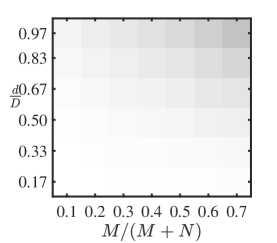
(a) $\phi_{0}$

(b) $\phi^{\natural}$ in (23)

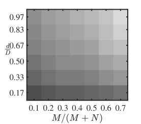
(c) $\phi^{\star}$ in (24)

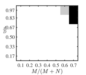
(d) check (23)

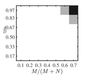
(e) check (24)

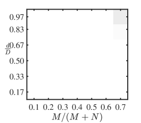
(f) $\phi_{1}$

(g) $\phi_{2}$

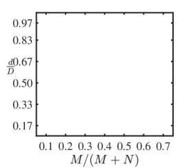
(h) $\phi_{3}$

Figure 5: (a) the angle $\phi_{0}$ ($0^{\circ}$ corresponds to black and $90^{\circ}$ corresponds to white) of $\widehat{\boldsymbol{b}}_{0}$ from the subspace $\mathcal{S}$ where $\boldsymbol{b}_{0}$ is obtained via the spectral method in 3, (b) the angle $\phi^{\star}$ in (23), (c) the angle $\phi^{\natural}$ in (24), (d) whether the sufficient condition (23) is satisfied (white if $\phi_{0}>\phi^{\natural}$) or not (black if $\phi_{0}\leq\phi^{\natural}$), (e) whether the sufficient condition (24) is satisfied (white if $\phi_{0}>\phi^{\star}$) or not (black if $\phi_{0}\leq\phi^{\star}$), (f) the angle $\phi_{1}$ of $\widehat{\boldsymbol{b}}_{1}$ in (22), (g) the angle $\phi_{2}$ of $\widehat{\boldsymbol{b}}_{2}$ in (22), (h) the angle $\phi_{3}$ of $\widehat{\boldsymbol{b}}_{3}$ in (22). Here, the vertical axis is the relative inlier subspace dimension $\frac{d}{D}$, while the horizontal axis represents the outlier ratio. The dimension of the ambient space is $D=30$ and the number of inliers is $N=500$. Results are averaged over 10 independent trails.

(a) $\phi_{0}$

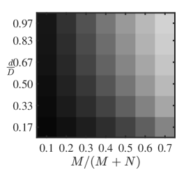
(b) $\phi^{\natural}$ in (23)

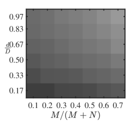
(c) $\phi^{\star}$ in (24)

(d) check (23)

(e) check (24)

(f) $\phi_{1}$

Figure 6: Similar to Figure 5 except that $N=1500$.

5.2 Demonstration of the Convergence of the PSGM

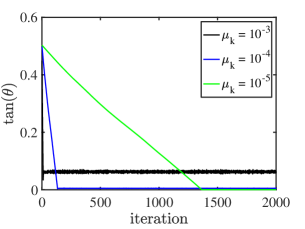
(a)

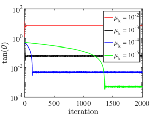
(b)

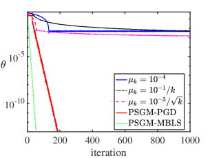
(c)

Figure 7: Convergence of PSGM with (a) constant step sizes (in the normal scale), (b) constant step sizes (in the log scale), (c) different choices of diminishing step sizes. We omit the result for $\mu_{k}=10^{-2}$ in (a) because it results in a relatively large $\theta$. Here $D=30,d=29,N=500,\frac{M}{M+N}=0.7$.

We now use synthetic experiments to verify the proposed PSGM algorithms. Similar to the previous setup, we fix $D=30$, randomly sample a subspace $\mathcal{S}$ of dimension $d=29$, and uniformly at random sample $N=500$ inliers and $M=1167$ outliers (so that the outlier ratio $M/(M+N)=0.7$) with unit $\ell_{2}$-norm. Inspired by the Piecewise Geometrically Diminishing (PGD) step sizes, we also use a modified backtracking line search (MBLS) that always uses the previous step size as an initialization for finding the current one within a backtracking line search (Nocedal and Wright, 2006, Section 3.1) strategy, which dramatically reduces the computational time compared with a standard backtracking line search. The corresponding algorithm is denoted by PSGM-MBLS. We set $K_{0}=30$, $K=4$ and $\beta=1/2$ for PGD step sizes with initial step size obtained by one iteration of a backtracking line search and denote the corresponding algorithm by PSGM-PGD. We define $\widehat{\boldsymbol{b}}_{0}$ to be the bottom eigenvector of $\widetilde{\mathbfcal}{X}\widetilde{\mathbfcal}{X}^{\top}$. Figure 7 displays the convergence of the PSGM (see Algorithm 1) with different choices of step sizes. As we observed from Figure 7(a) on the constant step sizes, at the begining $\tan(\theta_{k})$ decreases almost at a certain rate (which is proportional to $\mu_{k}=\mu$) in each iteration until it reaches a certain level (that is also proportional to $\mu_{k}=\mu$), and then it bounds around under this level, in coincidence with the analysis in 4. Figure 7(c) shows the convergence of the PSGM with different choices of diminishing step sizes. We observe linear convergence for both PSGM-PGD and PSGM-MBLS, which converge much faster than PSGM with constant step sizes or classical diminishing step sizes.

We use synthetic experiments under different settings to further verify the proposed PSGM algorithm with piecewise exponentionally diminishing step sizes. Figure 8 displays the convergence of $\theta$ (to $0$) with different $d$, $D$, $N$ and outlier ratio $\gamma$. In particular, Figure 8(a) shows the convergence of $\theta$ with $D=30,N=500,\gamma=0.7$ and different subspace dimension $d$. We observe $R$-linear convergence in this case, irrespectively the subspace dimension $d$. Figure 8(d) displays similar results but with larger $D$ and $N$. In Figure 8(b), we set $D=30,d=29,N=500$ and vary the outlier ratio $\gamma$ from $0.1$ to $0.9$. We observe $R$-linear convergence expept for the case $\gamma=0.9$, in which we have much more outliers than inliers. Interestingly, as shown in Figure 8(e), when we increase to $N=1500$ and keep the other parameters the same as in Figure 8(b), the PSGM algorithm has $R$-linear convergence even for $\gamma=0.9$. This coincides with the fact that the larger $N$, the more likely the condition (52) is satisfied. Finally we display experiments with varied $N$ in Figure 8(c) and Figure 8(f). We also observe $R$-linear convergence for PSGM with piecewise exponentionally diminishing step sizes given sufficient number of inliers.

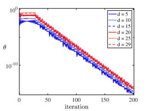
(a) $D=30,N=500,\gamma=0.7$

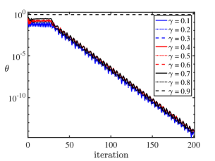
(b) $D=30,d=29,N=500$

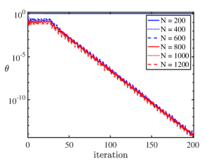
(c) $D=30,d=29,M=1000$

(d) $D=300,N=5000,\gamma=0.7$

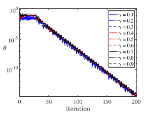
(e) $D=30,d=29,N=1500$

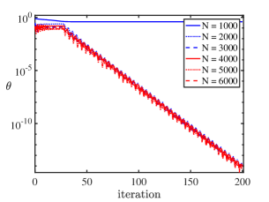
(f) $D=100,d=299,M=3000$

Figure 8: Convergence of the PSGM with piecewise exponentionally diminishing step size with $K_{0}=30,K=4$, $\beta=\frac{1}{2}$, and $\mu_{0}$ determined by line search method. Here $\gamma=\frac{M}{M+N}$ denotes the outlier ratio.

In Figure 9(a) and Figure 9(b) we compare PSGM algorithms with the ALP method (DPCP-ALP) and the IRLS algorithm (DPCP-IRLS) proposed in (Tsakiris and Vidal, 2017a). First observe that, as expected, although ALP finds a normal vector in few iterations, it has the highest time complexity because it solves an LP during each iteration. Figure 9(b) indicates that one iteration of ALP consumes more time than the whole procedure for PSGM. We also note that aside from the theoretical guarantee for PSGM-PGD, it also converges faster than IRLS (in terms of computing time), which lacks a convergence guarantee.

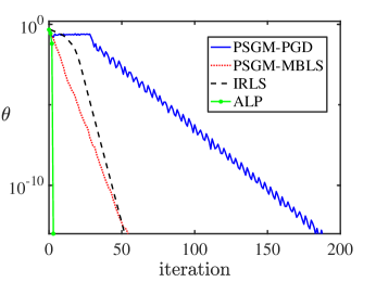
(a)

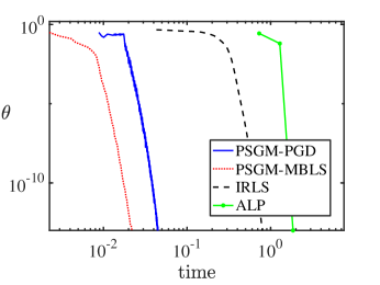
(b)

Figure 9: Comparison of PSGM with ALP and IRLS in (Tsakiris and Vidal, 2017a) in terms of (a) iterations and (b) computing time. Here $D=30,d=29,N=500,\frac{M}{M+N}=0.7$.

5.3 Phase Transition in Terms of $M$ and $N$

Using the same setup for generating outliers and inliers, we fix the ambient dimension $D=30$ and the subspace dimension $d$ and vary the number of outliers $M$ and the number of inliers $N$ to illustrate 2. Figure 10 displays the principal angle from $\mathcal{S}^{\perp}$ of the solution to the DPCP problem computed by the PSGM-MBLS algorithm for $d=15$ and $d=29$. We observe that the phase transition is indeed quadratic, indicating that DPCP can tolerate as many as $O(N^{2})$ outliers as predicted by 2. The relationship between $M$ and $d$ can also be observed by comparing Figure 10(a) with Figure 10(b). Particularly, we can see that when fix the ambient dimension $D$ and the number of inliers $N$, the subspace with smaller ambient dimension $d$ can tolerate more outliers, coincidence with $M=O(\frac{N^{2}}{d})$ outliers in 2.

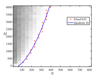
(a) $d=15$

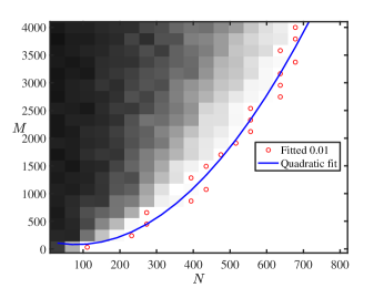
(b) $d=29$

Figure 10: The principal angle $\theta$ between the solution to the DPCP problem (6) and $\mathcal{S}^{\perp}$ (black corresponds to $\frac{\pi}{2}$ and white corresponds to $0$) when $D=30$ and (a) $d=15$ and (b) $d=29$. For each $M$, we find the smallest $N$ (red dots) such that $\theta\leq 0.01$. The blue quadratic curve indicates the least-squares fit to these points. Results are averaged over 10 independent trails.

5.4 Experiments on Real $3$D Point Cloud Road Data

We compare DPCP-PSGM (with a modified backtracking line search) with RANSAC Fischler and Bolles (1981), $\ell_{2,1}$-RPCA Xu et al. (2010) and REAPER Lerman et al. (2015a) on the road detection challenge of the KITTI dataset  Geiger et al. (2013), recorded from a moving platform while driving in and around Karlsruhe, Germany. This dataset consists of image data together with corresponding $3$D points collected by a rotating 3D laser scanner. In this experiment we use only the $360^{\circ}$ $3$D point clouds with the objective of determining the $3$D points that lie on the road plane (inliers) and those off that plane (outliers). Typically, each $3$D point cloud is on the order of $100,\!000$ points including about $50\%$ outliers. Using homogeneous coordinates this can be cast as a robust hyperplane learning problem in $\mathbb{R}^{4}$. Since the dataset is not annotated for that purpose, we manually annotated a few frames (e.g., see the left column of Fig. 11). Since DPCP-PSGM is the fastest method (on average converging in about $100$ milliseconds for each frame on a $6$ core $6$ thread Intel (R) i$5$-$8400$ machine), we set the time budget for all methods equal to the running time of DPCP-PSGM. For RANSAC we also compare with 10 and 100 times that time budget. Since $\ell_{2,1}$-RPCA does not directly return a subspace model, we extract the normal vector via SVD on the low-rank matrix returned by that method. Table 2 reports the area under the Receiver Operator Curve (ROC), the latter obtained by thresholding the distances of the points to the hyperplane estimated by each method, using a suitable range of different thresholds. As seen, even though a low-rank method, $\ell_{2,1}$-RPCA performs reasonably well but not on par with DPCP-PSGM and REAPER, which overall tend to be the most robust methods. On the contrary, for the same time budget, RANSAC, which is a popular choice in the computer vision community for such outlier detection tasks, is essentially failing due to an insufficient number of iterations. Even allowing for a $100$ times higher time budget still does not make RANSAC the best method, as it is outperformed by DPCP-PSGM on five out of the seven point clouds (1, 45, and 137 in KITTY-CITY-5, and 0 and 21 in KITTY-CITY-48).

Table 2: Area under ROC for annotated $3$D point clouds with index 1, 45, 120, 137, 153 in KITTY-CITY-5 and 0, 21 in KITTY-CITY-48. The number in parenthesis is the percentage of outliers.

			KITTY-CITY-5					KITTY-CITY-48
Methods		1(37%)	45(38%)	120(53%)	137(48%)	153(67%)		0(56%)	21(57%)
DPCP-PSGM		0.998	0.999	0.868	1.000	0.749		0.994	0.991
REAPER		0.998	0.998	0.839	0.999	0.749		0.994	0.982
$\ell_{2,1}$-RPCA		0.841	0.953	0.610	0.925	0.575		0.836	0.837
RANSAC		0.596	0.592	0.569	0.551	0.521		0.534	0.531
10xRANSAC		0.911	0.773	0.717	0.654	0.624		0.757	0.598
100xRANSAC		0.991	0.983	0.965	0.955	0.849		0.974	0.902

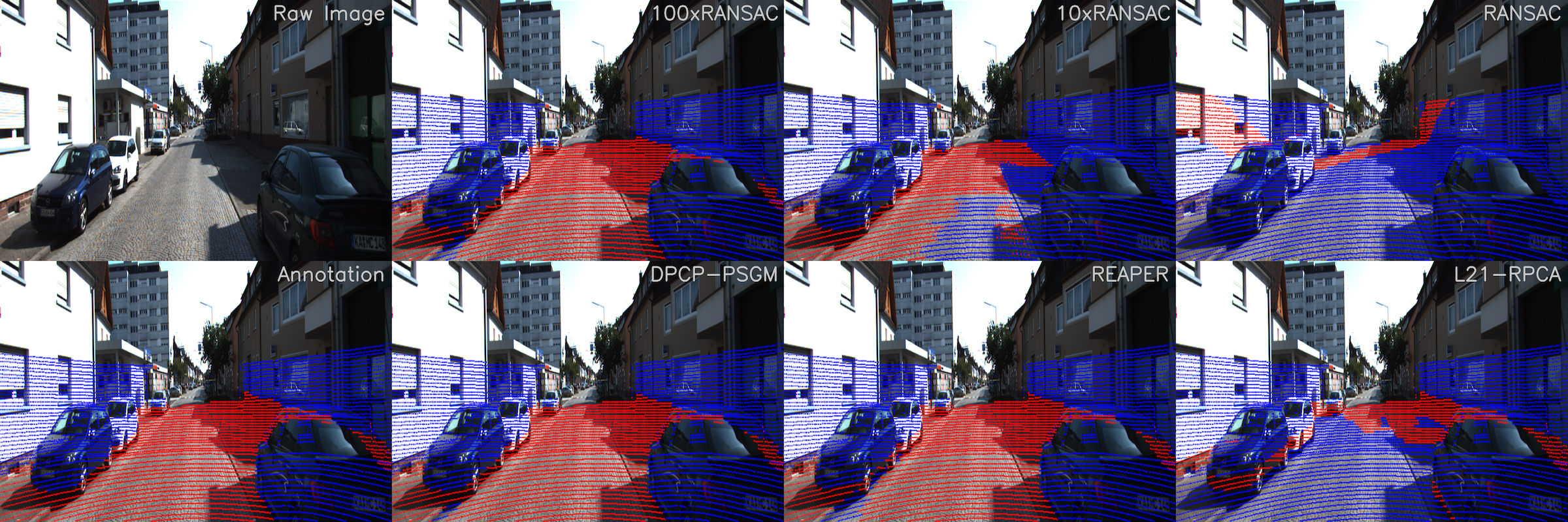
Figure 11: Frame $21$ of dataset KITTI-CITY-48: raw image, projection of annotated $3$D point cloud onto the image, and detected inliers/outliers using a ground-truth threshold on the distance to the hyperplane for each method. The corresponding F$1$ measures are DPCP-PSGM (0.933), REAPER (0.890), $\ell_{21}$-RPCA (0.248), RANSAC (0.023), 10xRANSAC (0.622), and 100xRANSAC (0.824).

6 Conclusions

We provided an improved analysis for the global optimality of the Dual Principal Component Pursuit (DPCP) method, which in particular suggests that DPCP can handle up to $O((\#\text{inliers})^{2})$ outliers. We also presented a scalable first-order method that only uses matrix-vector multiplications, for which we established global convergence guarantees for various step size selection schemes, regardless of the non-convexity and non-smoothness of the DPCP optimization problem. Finally, experiments on $3$D point cloud road data demonstrate that DPCP-PSGM is able to outperform RANSAC when the latter is run with the same computational budget.

A Proof of 4

After presenting some useful preliminary results, we prove 4 by individually convering the four terms $c_{\mathbfcal{O},\min}$, $c_{\mathbfcal{O},\max}$, $\eta_{\mathbfcal{O}}$ and $\eta_{\mathbfcal{O}}$.

A.1 Preliminaries

Suppose $X_{1},\ldots,X_{n}$ are $n$ independent and identically distributed (i.i.d.) random observations from a probability measure $P$ on a measurable space $(\mathcal{X},\mathcal{A})$. Given a measurable function $f:\mathcal{X}\rightarrow\mathbb{R}$, the empirical process evaluated at $f$ is defined as

$$\mathbb{G}_{n}f:=\sqrt{n}\left(\frac{1}{n}\sum_{i=1}^{n}f(X_{i})-\int f\operatorname{d}P\right),$$ (78)

where $\int f\operatorname{d}P$ is the expectation of $f$ under $P$ and $\frac{1}{n}\sum_{i=1}^{n}f(X_{i})$ is called the empirical distribution. There are several results concerning the supreme of $\mathbb{G}_{n}f$ over a given class $\mathcal{F}$ of measurable functions.

Define an envelope function $F:\mathcal{X}\rightarrow\mathbb{R}$ such that $|f|\leq F$ for every $f\in\mathcal{F}$. The $L_{r}(P)$-norm is defined as $\|f\|_{L_{r}(P)}=(\int|f|^{r}\operatorname{d}P)^{1/r}$. We need one more definition for the so-called bracket number which (informally speaking) measures the size of a class functions $\mathcal{F}$. Given two functions $l$ and $u$, the bracket $[l,u]$ is the set of all functions $f$ with $l\leq f\leq u$. An $\epsilon$-bracket in $L_{r}(P)$ is a bracket $[l,u]$ with $\int(u-l)^{r}\operatorname{d}P\leq\epsilon^{r}$ (since $l\leq u$, it is equivalent to say $\|u-l\|_{L_{r}(P)}\leq\epsilon$). The bracket number $N_{[]}(\epsilon,\mathcal{F},L_{2}(P))$ is the minimum number of $\epsilon$-brackets needed to cover $\mathcal{F}$.

Lemma 7 ( (Van der Vaart, 1998), Cor. 19.35)

For any class $\mathcal{F}$ of measurable functions with envelope function $F$,

$$\mathbb{E}\left[\sup_{f\in\mathcal{F}}\left|\mathbb{G}_{n}f\right|\right]\lesssim J_{[]}(\|F\|_{P,2},\mathcal{F},L_{2}(P)),$$ (79)

where $J_{[]}(\|F\|_{P,2},\mathcal{F},L_{2}(P))$ is called the bracketing integral:

$$J_{[]}(\|F\|_{L_{2}(P)},\mathcal{F},L_{2}(P))=\int_{0}^{\|F\|_{L_{2}(P)}}\sqrt{\log\left(N_{[]}(\epsilon,\mathcal{F},L_{2}(P))\right)}\operatorname{d}\epsilon.$$ (80)

Lemma 8 (McDiarmid’s Inequality, (McDiarmid, 1989))

Let $Z_{1},\dots,Z_{n}$ be real-valued independent random variables. Let $f:\mathbb{R}^{n}\rightarrow\mathbb{R}$ be a function that satisfies

$$\sup_{z_{1},\cdots,z_{n},z_{i}^{\prime}}\Bigg{|}f(z_{1},\cdots,z_{i-1},z_{i},z_{i+1},\cdots,z_{n})-f(z_{1},\dots,z_{i-1},z_{i}^{\prime},z_{i+1},\cdots,z_{n})\Bigg{|}\leq c_{i},$$

for every $i=1,\cdots,n$. Then

$$\mathbb{P}\Bigg{[}\Bigg{|}f(Z_{1},\cdots,Z_{n})-\mathbb{E}\Bigg{[}f(Z_{1},\cdots,Z_{n})\Bigg{]}\Bigg{|}\geq\epsilon\Bigg{]}\leq 2\exp\Bigg{(}-\frac{2\epsilon^{2}}{\sum_{i=1}^{n}c_{i}^{2}}\Bigg{)}.$$

Lemma 9 (Rademacher Comparison, (Ledoux and Talagrand, 2013), Eqn. (4.20))

Let $F:\mathbb{R}\to\mathbb{R}$ be convex and increasing. Let $\varphi_{i}:\mathbb{R}\to\mathbb{R}$, $i\leq N$, be 1-Lipschitz functions such that $\varphi_{i}(0)=0$. Let $\varepsilon_{i}$ be Rademacher random variables. Then, for any bounded subset $T$ in $\mathbb{R}^{N}$

$$\mathbb{E}\Bigg{[}F\Bigg{(}\sup_{(t_{1},t_{2},\cdots,t_{N})\in T}\sum_{i=1}^{N}\varepsilon_{i}\varphi_{i}(t_{i})\Bigg{)}\Bigg{]}\leq\mathbb{E}\Bigg{[}F\Bigg{(}\sup_{(t_{1},t_{2},\cdots,t_{N})\in T}\sum_{i=1}^{N}\varepsilon_{i}t_{i}\Bigg{)}\Bigg{]}.$$ (81)

Lemma 10 (Rademacher Symmetrization, (Kakade, 2011), Thm. 1.1)

Let $F$ be a class of functions $f:\mathbb{R}\rightarrow\mathbb{R}$ such that $0\leq f(z)\leq 1$. Let $\varepsilon_{i}$ be Rademacher random variables. Then for independent and identically distributed random variables $Z_{1},\dots,Z_{n}$, we have

$$\mathbb{E}\Bigg{[}\sup_{f\in F}\Bigg{(}\frac{1}{n}\sum_{i=1}^{n}f(Z_{i})-\mathbb{E}[f(Z)]\Bigg{)}\Bigg{]} \leq 2\mathbb{E}\Bigg{[}\sup_{f\in F}\frac{1}{n}\sum_{i=1}^{n}\varepsilon_{i}f(Z_{i})\Bigg{]},$$ (82)

$$\mathbb{E}\Bigg{[}\sup_{f\in F}\Bigg{(}\mathbb{E}[f(Z)]-\frac{1}{n}\sum_{i=1}^{n}f(Z_{i})\Bigg{)}\Bigg{]} \leq 2\mathbb{E}\Bigg{[}\sup_{f\in F}\frac{1}{n}\sum_{i=1}^{n}\varepsilon_{i}f(Z_{i})\Bigg{]}.$$ (83)

We also require a standard result about the covering number of the sphere. Denote by $\mathcal{N}_{\epsilon}$ an $\epsilon$-net of $\mathbb{S}^{D-1}$ if every point $\boldsymbol{b}\in\mathbb{S}^{D-1}$ can be approximated to within $\epsilon$ by some point $\boldsymbol{b}^{\prime}\in\mathcal{N}_{\epsilon}$. The minimal cardinality of an $\epsilon$-net, denoted by $\mathcal{N}(\mathbb{S}^{D-1},\epsilon)$, is called the covering number of $\mathbb{S}^{D-1}$.

Lemma 11

(Covering Number of the Sphere, (Vershynin, 2010, Lemma 5.2)) For every $\epsilon>0$, the covering number of the sphere $\mathbb{S}^{D-1}$ satisfies

$$\mathcal{N}(\mathbb{S}^{D-1},\epsilon)\leq\left(1+\frac{2}{\epsilon}\right)^{D}.$$ (84)

We finally require one more result converning the probability that $\operatorname{sign}(\boldsymbol{o}^{\top}\boldsymbol{b})=\operatorname{sign}(\boldsymbol{o}^{\top}\boldsymbol{b}^{\prime})$ when $\boldsymbol{b}$ is very close to $\boldsymbol{b}^{\prime}$.

Lemma 12

Denote by $\mathbb{B}(\boldsymbol{b},\epsilon_{1})$ the set of points that around $\boldsymbol{b}$:

$$\mathbb{B}(\boldsymbol{b},\epsilon_{1}):=\left\{\boldsymbol{b}^{\prime}\in\mathbb{S}^{D-1}:\|\boldsymbol{b}-\boldsymbol{b}^{\prime}\|_{2}\leq\epsilon_{1}\right\}.$$

Let $\boldsymbol{o}\in\mathbb{S}^{D-1}$ be drawn independently and uniformaly at random from the unit sphere $\mathbb{S}^{D-1}$. For any $\boldsymbol{b}\in\mathbb{S}^{D-1}$ and $\epsilon>0$, define

$$\overline{\mathbb{A}}:=\left\{\boldsymbol{o}\in\mathbb{S}^{D-1}:\operatorname{sign}(\boldsymbol{o}^{\top}\boldsymbol{b})=\operatorname{sign}(\boldsymbol{o}^{\top}\boldsymbol{b}^{\prime}),\ \forall\ \boldsymbol{b}^{\prime}\in\mathbb{B}(\boldsymbol{b},\epsilon_{1})\right\}.$$ (85)

Then

$$\operatorname{\mathbb{P}}\left[\boldsymbol{o}\in\overline{\mathbb{A}}^{c}\right]\lesssim\left\{\begin{matrix}\epsilon_{1},&D=2,\\ c_{D}D\epsilon_{1}^{2},&D\geq 3.\end{matrix}\right.$$

where $\lesssim$ means smaller than up to a universal constant which is independent of $D$.

Proof  Without loss of generality, suppose $\boldsymbol{b}=\boldsymbol{e}_{1}$ which is a length-$D$ vector with 1 in the first entry and 0 elsewhere. When $\epsilon_{1}>1$, note that $\mathbb{P}[\boldsymbol{o}\in\overline{\mathbb{A}}^{c}]\leq 1\lesssim c_{D}D\epsilon_{1}^{2}$. The rest is to consider the more interesting case that $\epsilon_{1}\leq 1$. Toward that end, first note that for any $\boldsymbol{b}^{\prime}\in\mathbb{B}(\boldsymbol{b},\epsilon_{1})$, we have $\boldsymbol{e}_{1}^{\top}\boldsymbol{b}^{\prime}\leq 1-\epsilon_{1}$, which further implies that $\operatorname{sign}(\boldsymbol{o}^{T}\boldsymbol{b}^{\prime})=\operatorname{sign}(\boldsymbol{o}^{\top}\boldsymbol{b})$ when $|o_{1}|\geq\epsilon_{1}$. Let $o_{1}$ be the first element in $\boldsymbol{o}$, we then have

$$\mathbb{P}\left[\overline{\mathbb{A}}^{c}\right] =\mathbb{P}\left[\left\{\boldsymbol{o}\in\mathbb{S}^{D-1}:\ \exists\ \boldsymbol{b}^{\prime}\in\mathbb{B}(\boldsymbol{b},\epsilon_{1}),\operatorname{sign}(\boldsymbol{o}^{\top}\boldsymbol{b})\neq\operatorname{sign}(\boldsymbol{o}^{\top}\boldsymbol{b}^{\prime})\right\}\right]$$

$$\leq\mathbb{P}\left[\left\{\boldsymbol{o}\in\mathbb{S}^{D-1}:o_{1}\in[-\epsilon_{1},\epsilon_{1}]\right\}\right]$$

To calculate the probability, we use the spherical coordinates. Denote by

$$\boldsymbol{o}=\begin{bmatrix}\cos(\theta_{1})\\ \sin(\theta_{1})\cos(\theta_{2})\\ \vdots\\ \sin(\theta_{1})\cdots\sin(\theta_{D-2})\cos(\theta_{D-1})\\ \sin(\theta_{1})\cdots\sin(\theta_{D-2})\sin(\theta_{D-1})\end{bmatrix},$$

where $\theta_{1},\cdots\theta_{D-2}\in[0,\pi)$ and $\theta_{D-1}\in[0,2\pi)$. Also let $I_{n}=\int_{0}^{\pi}\sin^{n}(\theta)\,\mathrm{d}\theta$. When $D>2$, let $\mathcal{A}$ be the area of the unit sphere. We have

$$\operatorname{\mathbb{P}}\left[\left\{\boldsymbol{o}\in\mathbb{S}^{D-1}:o_{1}\in[-\epsilon_{1},\epsilon_{1}]\right\}\right] =\frac{\int_{\mathbb{S}^{D-1}\cap o_{1}\in[-\epsilon_{1},\epsilon_{1}]}|\cos(\theta_{1})|\,\mathrm{d}\mathcal{A}}{\int_{\mathbb{S}^{D-1}}\,\mathrm{d}\mathcal{A}}$$

$$=\frac{2\int_{\arccos(\epsilon_{1})}^{\pi/2}\cos(\theta_{1})\sin^{D-2}(\theta_{1})\,\mathrm{d}\theta_{1}\prod_{j=1}^{D-3}I_{j}}{\prod_{j=1}^{D-2}I_{j}}$$

$$=\frac{2\int_{\arccos(\epsilon_{1})}^{\pi/2}\cos(\theta)\sin^{D-2}(\theta)\,\mathrm{d}\theta}{I_{D-2}}$$

$$=\frac{2\sin^{D-1}(\theta)\bigg{|}_{\arccos(\epsilon_{1})}^{\pi/2}}{(D-1)I_{D-2}}$$

$$=2\frac{1-(1-\epsilon_{1}^{2})^{(D-1)/2}}{(D-1)I_{D-2}}.$$

Note that

$$\frac{2}{(D-1)I_{D-2}} =\frac{1}{D-1}\cdot\frac{1}{\int_{0}^{\pi}\sin^{D-2}(\theta)\,\mathrm{d}\theta}$$

$$=\frac{1}{D-1}\cdot\frac{D-2}{D-3}\cdot\frac{1}{\int_{0}^{\pi}\sin^{D-4}(\theta)\,\mathrm{d}\theta}$$

$$=\frac{1}{D-1}\cdot\frac{D-2}{D-3}\cdot\frac{D-4}{D-5}\cdots$$

$$=c_{D}.$$

Then, applying Taylor’s approximation to the term $(1-\epsilon_{1}^{2})^{(D-1)/2}$ at $\epsilon_{1}=0$ gives

$$(1-\epsilon_{1}^{2})^{(D-1)/2} =1+0\cdot\epsilon_{1}+\frac{(D-1)(1-x^{2})^{\frac{D-1}{2}}((D-2)x^{2}-1)}{2(x^{2}-1)^{2}}\bigg{|}_{0}\epsilon_{1}^{2}+O(\epsilon_{1}^{3})$$

$$=1-\frac{D-1}{2}\epsilon_{1}^{2}+O(\epsilon_{1}^{3}).$$

Therefore, we have

$$\operatorname{\mathbb{P}}\left[\left\{\boldsymbol{o}\in\mathbb{S}^{D-1}:o_{1}\in[-\epsilon_{1},\epsilon_{1}]\right\}\right] =\frac{2}{(D-1)I_{D-2}}\cdot(1-(1-\epsilon_{1}^{2})^{(D-1)/2})$$

$$\lesssim c_{D}D\epsilon_{1}^{2}.$$

The proof of $D=2$ follows from a similar argument.  

A.2 Bounding $c_{\mathbfcal{O},\min}$

We first repeat the result in 4 concerning $c_{\mathbfcal{O},\min}$.

Lemma 13

Let $\boldsymbol{o}_{1},\dots,\boldsymbol{o}_{M}$ be uniformly distributed on $\mathbb{S}^{D-1}$. Then for any $t>0$

$$\mathbb{P}\Bigg{[}c_{\mathbfcal{O},\min}\leq c_{D}-\left(2+\frac{t}{2}\right)\frac{1}{\sqrt{M}}\Bigg{]}\leq 2\exp(-t^{2}/2).$$

Proof  We first present a useful result for proving 13.

Lemma 14

Let $\boldsymbol{o}_{1},\dots,\boldsymbol{o}_{M}$ be uniformly distributed on $\mathbb{S}^{D-1}$. Then

$$\mathbb{E}\Bigg{[}\sup_{||\boldsymbol{b}||_{2}=1}\Bigg{(}\sum_{j=1}^{M}|\boldsymbol{b}^{\top}\boldsymbol{o}_{j}|-c_{D}\Bigg{)}\Bigg{]} \leq\frac{2}{\sqrt{M}},$$

$$\mathbb{E}\Bigg{[}\sup_{||\boldsymbol{b}||_{2}=1}\Bigg{(}c_{D}-\sum_{j=1}^{M}|\boldsymbol{b}^{\top}\boldsymbol{o}_{j}|\Bigg{)}\Bigg{]} \leq\frac{2}{\sqrt{M}}.$$

Proof  Applying Lemma 10 using the class of functions $F=\{f_{\boldsymbol{b}}:\mathbb{S}^{D-1}\to\mathbb{R};f_{\boldsymbol{b}}(\boldsymbol{o})=|\boldsymbol{b}^{\top}\boldsymbol{o}|;\boldsymbol{b}\in\mathbb{S}^{D-1}\}$, we have

$$\mathbb{E}\Bigg{[}\sup_{||\boldsymbol{b}||_{2}=1}\Bigg{(}\sum_{j=1}^{M}|\boldsymbol{b}^{\top}\boldsymbol{o}_{j}|-c_{D}\Bigg{)}\Bigg{]} \leq\mathbb{E}\Bigg{[}\sup_{||\boldsymbol{b}||_{2}=1}\sum_{j=1}^{M}\varepsilon_{j}|\boldsymbol{b}^{\top}\boldsymbol{o}_{j}|\Bigg{]},$$

$$\mathbb{E}\Bigg{[}\sup_{||\boldsymbol{b}||_{2}=1}\Bigg{(}c_{D}-\sum_{j=1}^{M}|\boldsymbol{b}^{\top}\boldsymbol{o}_{j}|\Bigg{)}\Bigg{]} \leq\mathbb{E}\Bigg{[}\sup_{||\boldsymbol{b}||_{2}=1}\sum_{j=1}^{M}\varepsilon_{j}|\boldsymbol{b}^{\top}\boldsymbol{o}_{j}|\Bigg{]}.$$

Next, we apply Lemma 81 with $\varphi_{j}(\cdot)=|\cdot|$, $t_{j}=\boldsymbol{b}^{\top}\boldsymbol{o}_{j}$ to get the further bound

$$\mathbb{E}\Bigg{[}\sup_{||\boldsymbol{b}||_{2}=1}\sum_{j=1}^{M}\varepsilon_{j}|\boldsymbol{b}^{\top}\boldsymbol{o}_{j}|\Bigg{]} \leq 2\mathbb{E}\Bigg{[}\sup_{||\boldsymbol{b}||_{2}=1}\sum_{j=1}^{M}\varepsilon_{j}\boldsymbol{b}^{\top}\boldsymbol{o}_{j}\Bigg{]}=\frac{2}{M}\mathbb{E}\Bigg{[}\sup_{||\boldsymbol{b}||_{2}=1}\left\langle\boldsymbol{b},\sum_{j=1}^{M}\varepsilon_{j}\boldsymbol{o}_{j}\right\rangle\Bigg{]}$$

$$=\frac{2}{M}\mathbb{E}\left[\left|\left|\sum_{j=1}^{M}\varepsilon_{j}\boldsymbol{o}_{j}\right|\right|_{2}\right]\leq\frac{2}{M}\sqrt{\mathbb{E}\left[\left|\left|\sum_{j=1}^{M}\varepsilon_{j}\boldsymbol{o}_{j}\right|\right|_{2}^{2}\right]}$$

$$=\frac{2}{M}\sqrt{\mathbb{E}\left[M+\sum_{i\neq j}\varepsilon_{i}\varepsilon_{j}\boldsymbol{o}_{i}^{T}\boldsymbol{o}_{j}\right]}=\frac{2}{M}\sqrt{M}=\frac{2}{\sqrt{M}},$$

where the second inequality follows by $\mathbb{E}[Z]^{2}\leq\mathbb{E}[Z^{2}]$.  

We are now ready to prove 13. First note that

$$Mc_{\mathbfcal{O},\min}=\inf_{||\boldsymbol{b}||_{2}=1}\sum_{j=1}^{M}(|\boldsymbol{b}^{\top}\boldsymbol{o}_{j}|-c_{D})+Mc_{D}=Mc_{D}-\sup_{||\boldsymbol{b}||_{2}=1}\sum_{j=1}^{M}(c_{D}-|\boldsymbol{b}^{\top}\boldsymbol{o}_{j}|).$$

Applying Lemma 14, we have

$$\mathbb{E}\Bigg{[}\sup_{||\boldsymbol{b}||_{2}=1}\sum_{j=1}^{M}(c_{D}-|\boldsymbol{b}^{\top}\boldsymbol{o}_{j}|)\Bigg{]}\leq 2\sqrt{M}.$$

Applying Lemma 8 the same way as in proof of Theorem 15, we have

$$\mathbb{P}\Bigg{[}\sup_{||\boldsymbol{b}||_{2}=1}\sum_{j=1}^{M}(c_{D}-|\boldsymbol{b}^{\top}\boldsymbol{o}_{j}|)\geq 2\sqrt{M}+\epsilon\Bigg{]}\leq 2\exp(-2\epsilon^{2}/M).$$

Therefore,

$$\mathbb{P}\Bigg{[}Mc_{D}-\sup_{||\boldsymbol{b}||_{2}=1}\sum_{j=1}^{M}(c_{D}-|\boldsymbol{b}^{\top}\boldsymbol{o}_{j}|)\leq Mc_{D}-2\sqrt{M}-\epsilon\Bigg{]}\leq 2\exp(-2\epsilon^{2}/M),$$

and setting $\epsilon=t\sqrt{M}/2$ we get

$$\mathbb{P}\Bigg{[}Mc_{\mathbfcal{O},\min}\leq Mc_{D}-\left(2+\frac{t}{2}\right)\sqrt{M}\Bigg{]}\leq 2\exp(-t^{2}/2).$$

 

A.3 Bounding $c_{\mathbfcal{O},\max}$

We first repeat the result in 4 concerning $c_{\mathbfcal{O},\max}$.

Lemma 15

Let $\boldsymbol{o}_{1},\dots,\boldsymbol{o}_{M}$ be uniformly distributed on $\mathbb{S}^{D-1}$. Then for any $t>0$

$$\mathbb{P}\Bigg{[}c_{\mathbfcal{O},\max}\geq c_{D}+\left(2+\frac{t}{2}\right)\frac{1}{\sqrt{M}}\Bigg{]}\leq 2\exp(-t^{2}/2).$$

Proof  First note that

$$Mc_{\mathbfcal{O},\max}=\sup_{||\boldsymbol{b}||_{2}=1}\sum_{j=1}^{M}(|\boldsymbol{b}^{\top}\boldsymbol{o}_{j}|-c_{D})+Mc_{D}.$$

Since $\mathbb{S}^{D-1}$ is compact, there exists $\boldsymbol{b}^{*}\in\mathbb{S}^{D-1}$ which achieves the supremum in the expression above. Then for any $\boldsymbol{v}_{1},\boldsymbol{v}_{2},\cdots,\boldsymbol{v}_{M},\boldsymbol{v}_{k}^{\prime}\in\mathbb{S}^{D-1}$, we have

$$\Bigg{|}\sup_{||\boldsymbol{b}||_{2}=1}\sum_{j=1}^{M}(|\boldsymbol{b}^{\top}\boldsymbol{v}_{j}|-c_{D})-\sup_{||\boldsymbol{b}||_{2}=1}\Bigg{(}\sum_{j\neq k}(|\boldsymbol{b}^{\top}\boldsymbol{v}_{j}|-c_{D})+|\boldsymbol{b}^{\top}\boldsymbol{v}_{k}^{\prime}|-c_{D}\Bigg{)}\Bigg{|}$$

$$\leq\Bigg{|}\sum_{j=1}^{M}(|\boldsymbol{b^{*}}^{\top}\boldsymbol{v}_{j}|-c_{D})-\Bigg{(}\sum_{j\neq k}(|\boldsymbol{b^{*}}^{\top}\boldsymbol{v}_{j}|-c_{D})+|\boldsymbol{b^{*}}^{\top}\boldsymbol{v}_{k}^{\prime}|-c_{D}\Bigg{)}\Bigg{|}$$

$$=\Bigg{|}|\boldsymbol{b^{*}}^{\top}\boldsymbol{v}_{k}|-|\boldsymbol{b^{*}}^{\top}\boldsymbol{v}_{k}^{\prime}|\Bigg{|}\leq 1.$$

Applying Lemma 8 with $c_{k}=1$ and using Lemma 14, we obtain

$$\mathbb{P}\Bigg{[}\sup_{||\boldsymbol{b}||_{2}=1}\sum_{j=1}^{M}(|\boldsymbol{b}^{\top}\boldsymbol{o}_{j}|-c_{D})\geq 2\sqrt{M}+\epsilon\Bigg{]}\leq 2\exp(-2\epsilon^{2}/M).$$

Finally, set $\epsilon=t\sqrt{M}/2$ to get

$$\mathbb{P}\Bigg{[}Mc_{\mathbfcal{O},\max}\geq Mc_{D}+\left(2+\frac{t}{2}\right)\sqrt{M}\Bigg{]}\leq 2\exp(-t^{2}/2).$$

 

A.4 Bounding $c_{\mathbfcal{X},\min}$

The proof of the result concerning $c_{\mathbfcal{X},\min}$ in 4 follows similar argument as the one for $c_{\mathbfcal{O},\min}$ in Section A.2.

A.5 Bounding $\eta_{\mathbfcal{O}}$

Recall that $\eta_{\mathbfcal{O}}$ defined in (10) is equivalent to

$$\eta_{\mathbfcal{O}}=\frac{1}{M}\max_{\boldsymbol{g},\boldsymbol{b}\in\mathbb{S}^{D-1},\boldsymbol{g}\perp\boldsymbol{b}}\ \left|\boldsymbol{g}^{\top}\mathbfcal{O}\operatorname{sign}(\mathbfcal{O}^{\top}\boldsymbol{b})\right|.$$

We repeat the result in 4 concerning the above $\eta_{\mathbfcal{O}}$.

Lemma 16

Let $\boldsymbol{o}_{1},\dots,\boldsymbol{o}_{M}$ be uniformly distributed on $\mathbb{S}^{D-1}$. Then for any $t>0$

$$\mathbb{P}\Bigg{[}\sup_{\boldsymbol{b},\boldsymbol{g}\in\mathbb{S}^{D-1},\boldsymbol{b}\bot\boldsymbol{g}}\Bigg{|}\sum_{j=1}^{M}\operatorname{sign}(\boldsymbol{b}^{\top}\boldsymbol{o}_{j})\boldsymbol{g}^{\top}\boldsymbol{o}_{j}\Bigg{|}\gtrsim(1+t)\sqrt{D}\log\left(\sqrt{c_{D}D}\right)\sqrt{M}\Bigg{]}\leq 2\exp(-t^{2}/2).$$ (86)

Proof  Before givin out the main proofs, we first preset the following useful result concerning the expectation of $\eta_{\mathbfcal{O}}$.

Lemma 17

Suppose $\boldsymbol{o}_{1},\cdots,\boldsymbol{o}_{M},$ are drawn independently and uniformly at random from the unit sphere $\mathbb{S}^{D-1}$. Then

$$\mathbb{E}\Bigg{[}\sup_{\boldsymbol{b},\,\boldsymbol{g}\in\mathbb{S}^{D-1},\,\boldsymbol{b}\perp\boldsymbol{g}}\left|\sum_{j=1}^{M}\operatorname{sign}(\boldsymbol{b}^{\top}\boldsymbol{o}_{j})\boldsymbol{g}^{\top}\boldsymbol{o}_{j}\right|\Bigg{]}\lesssim\sqrt{D}\log\left(\sqrt{c_{D}D}\right)\sqrt{M},$$ (87)

where $\lesssim$ means smaller than up to a universal constant which is independent of $D$ and $M$.

Proof  The main idea for proving 17 is to view

$$\frac{1}{\sqrt{M}}\sup_{\boldsymbol{b},\,\boldsymbol{g}\in\mathbb{S}^{D-1},\,\boldsymbol{b}\perp\boldsymbol{g}}\left|\sum_{j=1}^{M}\operatorname{sign}(\boldsymbol{b}^{\top}\boldsymbol{o}_{j})\boldsymbol{g}^{\top}\boldsymbol{o}_{j}\right|$$

as an empirical process and then utilize Equation 80. Towards that end, define the set

$$\mathbb{F}:=\left\{(\boldsymbol{b},\boldsymbol{g}):\boldsymbol{b},\boldsymbol{g}\in\mathbb{S}^{D-1},\boldsymbol{b}\perp\boldsymbol{g}\right\}.$$

We further define the parameterized function as

$$f_{\boldsymbol{b},\boldsymbol{g}}(\boldsymbol{o}):=\operatorname{sign}(\boldsymbol{b}^{\top}\boldsymbol{o})\boldsymbol{g}^{\top}\boldsymbol{o}.$$

The class of functions we are interested in is $\mathcal{F}:=\left\{f_{\boldsymbol{b},\boldsymbol{g}}:(\boldsymbol{b},\boldsymbol{g})\in\mathbb{F}\right\}$.

Note that for any $f_{\boldsymbol{b},\boldsymbol{g}}\in\mathcal{F}$ (i.e., $(\boldsymbol{b},\boldsymbol{g})\in\mathbb{F}$), we have

$$\mathbb{E}\left[f_{\boldsymbol{b},\boldsymbol{g}}(\boldsymbol{o})\right]=\mathbb{E}\left[\operatorname{sign}(\boldsymbol{b}^{\top}\boldsymbol{o})\boldsymbol{g}^{\top}\boldsymbol{o}\right]=0,$$

which together with (78) indicates that

$$\sum_{j=1}^{M}\operatorname{sign}(\boldsymbol{b}^{\top}\boldsymbol{o}_{j})\boldsymbol{g}^{\top}\boldsymbol{o}_{j}=\sqrt{M}\mathbb{G}_{M}f_{\boldsymbol{b},\boldsymbol{g}},$$

where $\mathbb{G}_{M}f_{\boldsymbol{b},\boldsymbol{g}}$ is the empirical process of $f_{\boldsymbol{b},\boldsymbol{g}}$.

To utilize Equation 80, the rest of the proof is to show the corresponding bracketing integral is finite for our problem. Since $|f_{\boldsymbol{b},\boldsymbol{g}}(\boldsymbol{o})|\leq\|\boldsymbol{o}\|_{2}$ for any $(\boldsymbol{b},\boldsymbol{g})\in\mathbb{F}$, we know $F(\boldsymbol{o})=\|\boldsymbol{o}\|_{2}$ is the envelope function of $\mathcal{F}$ and $\|F\|_{P,2}=1$. Thus, we only need to consider the the bracket integral $J_{[]}(1,\mathcal{F},L_{2}(P))$, where $P$ is now a probability measure on the unit sphere. To that end, we first compute the bracket number $N_{[]}(\epsilon,\mathcal{F},L_{2}(P))$.

Since our function $f_{\boldsymbol{b},\boldsymbol{g}}$ is parameterized by $(\boldsymbol{b},\boldsymbol{g})$, covering the class of functions $\mathcal{F}$ is related to covering the set $\mathbb{F}$. For any fixed $(\boldsymbol{b},\boldsymbol{g})\in\mathbb{F}$, define the set of points that around $(\boldsymbol{b},\boldsymbol{g})$:

$$\mathbb{B}((\boldsymbol{b},\boldsymbol{g}),\epsilon_{1}):=\left\{(\boldsymbol{b}^{\prime},\boldsymbol{g}^{\prime})\in\mathbb{F}:\sqrt{\|\boldsymbol{b}-\boldsymbol{b}^{\prime}\|_{2}^{2}+\|\boldsymbol{g}-\boldsymbol{g}^{\prime}\|_{2}^{2}}\leq\epsilon_{1}\right\}.$$

Then, denote by

$$\mathbb{A}:=\left\{\boldsymbol{o}\in\mathbb{R}^{D}:\operatorname{sign}(\boldsymbol{o}^{\top}\boldsymbol{b})=\operatorname{sign}(\boldsymbol{o}^{\top}\boldsymbol{b}^{\prime}),\ \forall\ (\boldsymbol{b}^{\prime},\boldsymbol{g}^{\prime})\in\mathbb{B}((\boldsymbol{b},\boldsymbol{g}),\epsilon_{1})\right\}.$$

When $\boldsymbol{b}$ is close to $\boldsymbol{b}^{\prime}$, then $\mathbb{A}$ should cover most of $\boldsymbol{o}$. If $\boldsymbol{o}\in\mathbb{A}$, then for any $(\boldsymbol{b}^{\prime},\boldsymbol{g}^{\prime})\in\mathbb{B}((\boldsymbol{b},\boldsymbol{g}),\epsilon_{1})$ we have

$$|f_{\boldsymbol{b},\boldsymbol{g}}(\boldsymbol{o})-f_{\boldsymbol{b}^{\prime},\boldsymbol{g}^{\prime}}(\boldsymbol{o})|=|\boldsymbol{o}^{\top}(\boldsymbol{g}-\boldsymbol{g}^{\prime})|\leq\|\boldsymbol{g}-\boldsymbol{g}^{\prime}\|_{2}\|\boldsymbol{o}\|_{2}\leq\epsilon_{1}.$$

On the other hand, if $\boldsymbol{o}\in\mathbb{A}^{c}$, then for any $(\boldsymbol{b}^{\prime},\boldsymbol{g}^{\prime})\in\mathbb{B}((\boldsymbol{b},\boldsymbol{g}),\epsilon_{1})$ we have

$$|f_{\boldsymbol{b},\boldsymbol{g}}(\boldsymbol{o})-f_{\boldsymbol{b}^{\prime},\boldsymbol{g}^{\prime}}(\boldsymbol{o})|=|\boldsymbol{o}^{\top}(\boldsymbol{g}+\boldsymbol{g}^{\prime})|\leq\|\boldsymbol{g}+\boldsymbol{g}^{\prime}\|_{2}\|\boldsymbol{o}\|_{2}\leq 2.$$

To summary, we have

$$|f_{\boldsymbol{b},\boldsymbol{g}}(\boldsymbol{o})-f_{\boldsymbol{b}^{\prime},\boldsymbol{g}^{\prime}}(\boldsymbol{o})|\leq\epsilon_{1}\delta_{\mathbb{A}}(\boldsymbol{o})+2\delta_{\mathbb{A}^{c}}(\boldsymbol{o}),\ \forall\ (\boldsymbol{b}^{\prime},\boldsymbol{g}^{\prime})\in\mathbb{B}((\boldsymbol{b},\boldsymbol{g}),\epsilon_{1}).$$ (88)

We now define a bracket $[l,u]$ by

$$l(\boldsymbol{o})=f_{\boldsymbol{b},\boldsymbol{g}}(\boldsymbol{o})-\epsilon_{1}\delta_{\mathbb{A}}(\boldsymbol{o})-2\delta_{\mathbb{A}^{c}}(\boldsymbol{o}),$$

$$u(\boldsymbol{o})=f_{\boldsymbol{b},\boldsymbol{g}}(\boldsymbol{o})+\epsilon_{1}\delta_{\mathbb{A}}(\boldsymbol{o})+2\delta_{\mathbb{A}^{c}}(\boldsymbol{o}),$$

where the indicator function $\delta_{\mathbb{A}}(\boldsymbol{o})$ is defined as $\delta_{\mathbb{A}}(\boldsymbol{o})=\left\{\begin{matrix}1,&\boldsymbol{o}\in\mathbb{A}\\ 0,&\boldsymbol{o}\in\mathbb{A}^{c}\end{matrix}\right.$. Due to (88), we have $f_{\boldsymbol{b}^{\prime},\boldsymbol{g}^{\prime}}\in[l,u]$ for all $(\boldsymbol{b}^{\prime},\boldsymbol{g}^{\prime})\in\mathbb{B}((\boldsymbol{b},\boldsymbol{g}),\epsilon_{1})$. Also,

$$\begin{split}\|u-l\|_{L_{2}(P)}&=\|2\epsilon_{1}\delta_{\mathbb{A}}(\boldsymbol{o})+4\delta_{\mathbb{A}^{c}}(\boldsymbol{o})\|_{L_{2}(P)}=\sqrt{4\epsilon_{1}^{2}\mathbb{P}[\boldsymbol{o}\in\mathbb{A}]+16\mathbb{P}[\boldsymbol{o}\in\mathbb{A}^{c}]}\\ &<2\epsilon_{1}+4\sqrt{\mathbb{P}[\boldsymbol{o}\in\mathbb{A}^{c}]}\leq 2\epsilon_{1}+4\sqrt{\mathbb{P}[\boldsymbol{o}\in\overline{\mathbb{A}}^{c}]}\leq 2\epsilon_{1}+4\sqrt{c_{1}c_{D}D}\epsilon_{1},\end{split}$$ (89)

where $\overline{\mathbb{A}}$ is defined in (85), the second inequality utilizes the fact $\overline{\mathbb{A}}\subset\mathbb{A}$, $c_{1}$ is a universial constant, and the last inequality follows because $\mathbb{P}[\boldsymbol{o}\in\mathbb{A}^{c}]\leq c_{1}c_{D}D\epsilon_{1}^{2}$ according to 12 (we only consider $D>2$ here, but the proof for $D=2$ follows similarly).

Finally, the number of brackets to cover $\mathcal{F}$ is equal to the number of such balls $\mathbb{B}((\boldsymbol{b},\boldsymbol{g}),\epsilon_{1})$ that cover $\mathbb{F}$. Utilizing Equation 84, the covering number for $\mathbb{F}$ is

$$\mathcal{N}(\mathbb{F},\epsilon_{1})\leq\left(1+\frac{2\sqrt{2}}{\epsilon_{1}}\right)^{2D}.$$ (90)

Recall the definition that the bracket number $N_{[]}(\epsilon,\mathcal{F},L_{2}(P))$ is the minimum number of $\epsilon$-brackets needed to cover $\mathcal{F}$, where an $\epsilon$-bracket in $L_{2}(P)$ is a bracket $[l,u]$ with $\|u-l\|_{L_{2}(P)}\leq\epsilon$. Thus, by letting $2\epsilon_{1}+4\sqrt{c_{1}c_{D}D}\epsilon_{1}=\epsilon$ and plugging this into (90), we obtain the bracket number

$$N_{[]}(\epsilon,\mathcal{F},L_{2}(P))\leq\left(1+c_{2}\frac{\sqrt{c_{D}D}}{\epsilon}\right)^{2D},$$

where $c_{2}$ is a universal constant. Now plug this into Equation 80 gives

$$\frac{1}{\sqrt{M}}\mathbb{E}\Bigg{[}\sup_{\boldsymbol{b},\,\boldsymbol{g}\in\mathbb{S}^{D-1},\,\boldsymbol{b}\perp\boldsymbol{g}}\left|\sum_{j=1}^{M}\operatorname{sign}(\boldsymbol{b}^{\top}\boldsymbol{o}_{j})\boldsymbol{g}^{\top}\boldsymbol{o}_{j}\right|\Bigg{]} \lesssim\int_{0}^{1}\sqrt{\log\left(1+c_{2}\frac{\sqrt{c_{D}D}}{\epsilon}\right)^{2D}}\operatorname{d}\epsilon$$

$$\lesssim\sqrt{D}\log\left(\sqrt{c_{D}D}\right).$$

 

We are now ready to prove 16. For $\boldsymbol{v}_{1},\boldsymbol{v}_{2},\cdots,\boldsymbol{v}_{M},\boldsymbol{v}_{k}^{\prime}$ any points of $\mathbb{S}^{D-1}$, since the product of compact spaces is compact, there exist $\boldsymbol{b}^{*},\boldsymbol{g}^{*}\in\mathbb{S}^{D-1}$ for which the value

$$\sup_{\boldsymbol{b},\boldsymbol{g}\in\mathbb{S}^{D-1},\boldsymbol{b}\bot\boldsymbol{g}}|\sum_{j=1}^{M}\operatorname{sign}(\boldsymbol{b}^{\top}\boldsymbol{v}_{j})\boldsymbol{g}^{\top}\boldsymbol{v}_{j}|$$

is achieved. Then, we have

$$\left|\sup_{\boldsymbol{b},\boldsymbol{g}\in\mathbb{S}^{D-1},\boldsymbol{b}\bot\boldsymbol{g}}\left|\sum_{j=1}^{M}\operatorname{sign}(\boldsymbol{b}^{\top}\boldsymbol{v}_{j})\boldsymbol{g}^{\top}\boldsymbol{v}_{j}\right|-\sup_{\boldsymbol{b},\boldsymbol{g}\in\mathbb{S}^{D-1},\boldsymbol{b}\bot\boldsymbol{g}}\left|\sum_{j\neq k}\operatorname{sign}(\boldsymbol{b}^{\top}\boldsymbol{v}_{j})\boldsymbol{g}^{\top}\boldsymbol{v}_{j}+\operatorname{sign}(\boldsymbol{b}^{\top}\boldsymbol{v}_{k}^{\prime})\boldsymbol{g}^{\top}\boldsymbol{v}_{k}^{\prime}\right|\right|$$ (91)

$$\leq\left|\left|\sum_{j=1}^{M}\operatorname{sign}(\boldsymbol{b^{*}}^{\top}\boldsymbol{v}_{j})\boldsymbol{g^{*}}^{\top}\boldsymbol{v}_{j}\right|-\left|\sum_{j\neq k}\operatorname{sign}(\boldsymbol{b^{*}}^{\top}\boldsymbol{v}_{j})\boldsymbol{g^{*}}^{\top}\boldsymbol{v}_{j}+\operatorname{sign}(\boldsymbol{b^{*}}^{\top}\boldsymbol{v}_{k}^{\prime})\boldsymbol{g^{*}}^{\top}\boldsymbol{v}_{k}^{\prime}\right|\right|$$ (92)

$$\leq\Bigg{|}\operatorname{sign}(\boldsymbol{b}^{*\mathrm{T}}\boldsymbol{v}_{k})\boldsymbol{g^{*}}^{\top}\boldsymbol{v}_{k}-\operatorname{sign}(\boldsymbol{b^{*}}^{\top}\boldsymbol{v}_{k}^{\prime})\boldsymbol{g^{*}}^{\top}\boldsymbol{v}_{k}^{\prime}\Bigg{|}\leq 2,$$ (93)

where the second inequality follows from the reverse triangle inequality. Applying Lemma 8 with $c_{k}=2$ and using 17, we obtain

$$\mathbb{P}\Bigg{[}\sup_{\boldsymbol{b},\boldsymbol{g}\in\mathbb{S}^{D-1},\boldsymbol{b}\bot\boldsymbol{g}}\left|\sum_{j=1}^{M}\operatorname{sign}(\boldsymbol{b}^{\top}\boldsymbol{o}_{j})\boldsymbol{g}^{\top}\boldsymbol{o}_{j}\right|\gtrsim\sqrt{D}\log\left(\sqrt{c_{D}D}\right)\sqrt{M}+\epsilon\Bigg{]}\leq 2\exp\Bigg{(}-\frac{2\epsilon^{2}}{4M}\Bigg{)}.$$ (94)

Finally, set $\epsilon=t\sqrt{M}$ to get

$$\mathbb{P}\Bigg{[}\sup_{\boldsymbol{b},\boldsymbol{g}\in\mathbb{S}^{D-1},\boldsymbol{b}\bot\boldsymbol{g}}\left|\sum_{j=1}^{M}\operatorname{sign}(\boldsymbol{b}^{\top}\boldsymbol{o}_{j})\boldsymbol{g}^{\top}\boldsymbol{o}_{j}\right|\gtrsim\left(\sqrt{D}\log\left(\sqrt{c_{D}D}\right)+t\right)\sqrt{M}\Bigg{]}\leq 2\exp(-t^{2}/2).$$ (95)

 

B Proof of 5

To begin, we first assume that

$$\tan(\theta_{k})<\frac{Nc_{\mathbfcal{X},\min}}{N\eta_{\mathbfcal{X}}+M\eta_{\mathbfcal{O}}}$$ (96)

holds for all $k\geq 0$. As a consequence of (96), we have

$$\begin{split}\cos(\theta_{k})&=\frac{1}{\sqrt{1+\tan^{2}(\theta_{k})}}>\frac{1}{\sqrt{1+\left(\frac{Nc_{\mathbfcal{X},\min}}{N\eta_{\mathbfcal{X}}+M\eta_{\mathbfcal{O}}}\right)^{2}}}\geq\frac{1}{\sqrt{2}}\frac{N\eta_{\mathbfcal{X}}+M\eta_{\mathbfcal{O}}}{Nc_{\mathbfcal{X},\min}}\\ &=\frac{\mu^{\prime}(N\eta_{\mathbfcal{X}}+M\eta_{\mathbfcal{O}})}{\sqrt{2}\mu^{\prime}Nc_{\mathbfcal{X},\min}}\geq\frac{\mu^{\prime}(N\eta_{\mathbfcal{X}}+M\eta_{\mathbfcal{O}})}{(1-\mu^{\prime}Mc_{\mathbfcal{O},\max})},\end{split}$$ (97)

where the second inequality follows (52) that $N\eta_{\mathbfcal{X}}+M\eta_{\mathbfcal{O}}\leq Nc_{\mathbfcal{X},\min}$, and the last inequality utilizes (51) that $1-\mu^{\prime}Mc_{\mathbfcal{O},\max}\geq\frac{3}{4}\geq 3\mu^{\prime}Nc_{\mathbfcal{X},\min}$. With (96) and (97), we now prove the two main arguments in 5.

Case ($i$):

We first consider the case where $\theta_{k}$ is large compared with $\mu_{k}$:

$$\sin(\theta_{k-1})>\frac{\mu_{k}\|\mathbfcal{X}^{\top}\boldsymbol{s}_{k-1}\|_{1}}{(1-\mu_{k}\|\mathbfcal{O}^{\top}\widehat{\boldsymbol{b}}_{k-1}\|_{1})}.$$ (98)

It follows from (30) that

$$\begin{split}\boldsymbol{b}_{k}&=(1-\mu_{k}\|\mathbfcal{O}^{\top}\widehat{\boldsymbol{b}}_{k-1}\|_{1})\widehat{\boldsymbol{b}}_{k-1}-\mu_{k}\|\mathbfcal{X}^{\top}\boldsymbol{s}_{k-1}\|_{1}\boldsymbol{s}_{k-1}-\mu_{k}(\boldsymbol{p}_{k-1}+\boldsymbol{q}_{k-1})\\ &=\left((1-\mu_{k}\|\mathbfcal{O}^{\top}\widehat{\boldsymbol{b}}_{k-1}\|_{1})\sin(\theta_{k-1})-\mu_{k}\|\mathbfcal{X}^{\top}\boldsymbol{s}_{k-1}\|_{1}\right)\boldsymbol{s}_{k-1}\\ &\quad+(1-\mu_{k}\|\mathbfcal{O}^{\top}\widehat{\boldsymbol{b}}_{k-1}\|_{1})\cos(\theta_{k-1})\boldsymbol{n}_{k-1}-\mu_{k}(\boldsymbol{p}_{k-1}+\boldsymbol{q}_{k-1}),\end{split}$$

which furthr implies that

$$\begin{split}&\tan(\theta_{k})=\frac{\|\mathcal{P}_{\mathcal{S}}(\boldsymbol{b}_{k})\|_{2}}{\|\mathcal{P}_{\mathcal{S}^{\perp}}(\boldsymbol{b}_{k})\|_{2}}\\ &=\frac{\left\|\mathcal{P}_{\mathcal{S}}\left(\left((1-\mu_{k}\|\mathbfcal{O}^{\top}\widehat{\boldsymbol{b}}_{k-1}\|_{1})\sin(\theta_{k-1})-\mu_{k}\|\mathbfcal{X}^{\top}\boldsymbol{s}_{k-1}\|_{1}\right)\boldsymbol{s}_{k-1}-\mu_{k}(\boldsymbol{p}_{k-1}+\boldsymbol{q}_{k-1})\right)\right\|_{2}}{\left\|\mathcal{P}_{\mathcal{S}^{\perp}}\left((1-\mu_{k}\|\mathbfcal{O}^{\top}\widehat{\boldsymbol{b}}_{k-1}\|_{1})\cos(\theta_{k-1})\boldsymbol{n}_{k-1}-\mu_{k}(\boldsymbol{p}_{k-1}+\boldsymbol{q}_{k-1})\right)\right\|_{2}}\\ &\leq\frac{\left|(1-\mu_{k}\|\mathbfcal{O}^{\top}\widehat{\boldsymbol{b}}_{k-1}\|_{1})\sin(\theta_{k-1})-\mu_{k}\|\mathbfcal{X}^{\top}\boldsymbol{s}_{k-1}\|_{1}\right|+\mu_{k}\left\|\mathcal{P}_{\mathcal{S}}\left(\boldsymbol{p}_{k-1}+\boldsymbol{q}_{k-1}\right)\right\|_{2}}{(1-\mu_{k}\|\mathbfcal{O}^{\top}\widehat{\boldsymbol{b}}_{k-1}\|_{1})\cos(\theta_{k-1})-\mu_{k}\left\|\mathcal{P}_{\mathcal{S}^{\perp}}\left(\boldsymbol{p}_{k-1}+\boldsymbol{q}_{k-1}\right)\right\|_{2}}\\ &=\frac{(1-\mu_{k}\|\mathbfcal{O}^{\top}\widehat{\boldsymbol{b}}_{k-1}\|_{1})\sin(\theta_{k-1})-\mu_{k}\|\mathbfcal{X}^{\top}\boldsymbol{s}_{k-1}\|_{1}+\mu_{k}\left\|\mathcal{P}_{\mathcal{S}}\left(\boldsymbol{p}_{k-1}+\boldsymbol{q}_{k-1}\right)\right\|_{2}}{(1-\mu_{k}\|\mathbfcal{O}^{\top}\widehat{\boldsymbol{b}}_{k-1}\|_{1})\cos(\theta_{k-1})-\mu_{k}\left\|\mathcal{P}_{\mathcal{S}^{\perp}}\left(\boldsymbol{p}_{k-1}+\boldsymbol{q}_{k-1}\right)\right\|_{2}}\\ &=\frac{(1-\mu_{k}\|\mathbfcal{O}^{\top}\widehat{\boldsymbol{b}}_{k-1}\|_{1})\sin(\theta_{k-1})-\mu_{k}\|\mathbfcal{X}^{\top}\boldsymbol{s}_{k-1}\|_{1}+\mu_{k}\|\mathcal{P}_{\mathcal{S}}(\boldsymbol{p}_{k-1}+\boldsymbol{q}_{k-1})\|_{2}}{(1-\mu_{k}\|\mathbfcal{O}^{\top}\widehat{\boldsymbol{b}}_{k-1}\|_{1})\cos(\theta_{k-1})-\mu_{k}\|\boldsymbol{p}_{k-1}+\boldsymbol{q}_{k-1}\|_{2}+\mu_{k}\|\mathcal{P}_{\mathcal{S}}(\boldsymbol{p}_{k-1}+\boldsymbol{q}_{k-1})\|_{2}}.\end{split}$$ (99)

Based on the term $\Gamma_{1}:=\frac{(1-\mu_{k}\|\mathbfcal{O}^{\top}\widehat{\boldsymbol{b}}_{k-1}\|_{1})\sin(\theta_{k-1})-\mu_{k}\|\mathbfcal{X}^{\top}\boldsymbol{s}_{k-1}\|_{1}}{(1-\mu_{k}\|\mathbfcal{O}^{\top}\widehat{\boldsymbol{b}}_{k-1}\|_{1})\cos(\theta_{k-1})-\mu_{k}\|\boldsymbol{p}_{k-1}+\boldsymbol{q}_{k-1}\|_{2}}$, we further bound $\tan(\theta_{k})$ from above. In particular, when $\Gamma_{1}\leq 1$, we have (utilizing the fact that $\frac{a+x}{b+x}$ is an increasing function of $x$ when $x\geq 0$ and $0<a\leq b$)

$$\tan(\theta_{k})\leq\tan(\overline{\theta}_{k})=\frac{(1-\mu_{k}\|\mathbfcal{O}^{\top}\widehat{\boldsymbol{b}}_{k-1}\|_{1})\sin(\theta_{k-1})-\mu_{k}\|\mathbfcal{X}^{\top}\boldsymbol{s}_{k-1}\|_{1}+\mu_{k}\|\boldsymbol{p}_{k-1}+\boldsymbol{q}_{k-1}\|_{2}}{(1-\mu_{k}\|\mathbfcal{O}^{\top}\widehat{\boldsymbol{b}}_{k-1}\|_{1})\cos(\theta_{k-1})}$$

by plugging $\|\mathcal{P}_{\mathcal{S}}(\boldsymbol{p}_{k-1}+\boldsymbol{q}_{k-1})\|_{2}=\|\boldsymbol{p}_{k-1}+\boldsymbol{q}_{k-1}\|_{2}$ into the laste term in (99). When $\Gamma_{1}>1$, we have (utilizing the fact that $\frac{a+x}{b+x}$ is a decreasing function of $x$ when $x\geq 0$ and $a>b>0$)

$$\tan(\theta_{k})\leq\tan(\widetilde{\theta}_{k})=\frac{(1-\mu_{k}\|\mathbfcal{O}^{\top}\widehat{\boldsymbol{b}}_{k-1}\|_{1})\sin(\theta_{k-1})-\mu_{k}\|\mathbfcal{X}^{\top}\boldsymbol{s}_{k-1}\|_{1}}{(1-\mu_{k}\|\mathbfcal{O}^{\top}\widehat{\boldsymbol{b}}_{k-1}\|_{1})\cos(\theta_{k-1})-\mu_{k}\|\boldsymbol{p}_{k-1}+\boldsymbol{q}_{k-1}\|_{2}}$$

by plugging $\|\mathcal{P}_{\mathcal{S}}(\boldsymbol{p}_{k-1}+\boldsymbol{q}_{k-1})\|_{2}=0$ into the last term in (99). Combinging the above two cases together gives

$$\theta_{k}\leq\max\{\overline{\theta}_{k},\widetilde{\theta}_{k}\}.$$ (100)

In what follows, we obtain upper bounds for both $\overline{\theta}_{k}$ and $\widetilde{\theta}_{k}$. Towards that end, we first bound $\tan(\overline{\theta}_{k})$ from above as

$$\tan(\overline{\theta}_{k})=\frac{(1-\mu_{k}\|\mathbfcal{O}^{\top}\widehat{\boldsymbol{b}}_{k-1}\|_{1})\sin(\theta_{k-1})-\mu_{k}\|\mathbfcal{X}^{\top}\boldsymbol{s}_{k-1}\|_{1}+\mu_{k}\|\boldsymbol{p}_{k-1}+\boldsymbol{q}_{k-1}\|_{2}}{(1-\mu_{k}\|\mathbfcal{O}^{\top}\widehat{\boldsymbol{b}}_{k-1}\|_{1})\cos(\theta_{k-1})}$$

$$=\tan(\theta_{k-1})-\frac{\mu_{k}\|\mathbfcal{X}^{\top}\boldsymbol{s}_{k-1}\|_{1}-\mu_{k}\|\boldsymbol{p}_{k-1}+\boldsymbol{q}_{k-1}\|_{2}}{(1-\mu_{k}\|\mathbfcal{O}^{\top}\widehat{\boldsymbol{b}}_{k-1}\|_{1})\cos(\theta_{k-1})}$$

$$\leq\tan(\theta_{k-1})-\mu_{k}\frac{Nc_{\mathbfcal{X},\min}-(N\eta_{\mathbfcal{X}}+M\eta_{\mathbfcal{O}})}{(1-\mu_{k}Mc_{\mathbfcal{O},\min})\cos(\theta_{k-1})}$$

$$\leq\tan(\theta_{k-1})-\mu_{k}(Nc_{\mathbfcal{X},\min}-(N\eta_{\mathbfcal{X}}+M\eta_{\mathbfcal{O}})),$$

where the last inequality follows because $0<1-\mu_{k}Mc_{\mathbfcal{O},\min}\leq 1$. Thus,

$$\tan(\theta_{k-1})-\tan(\overline{\theta}_{k})\geq\mu_{k}(Nc_{\mathbfcal{X},\min}-(N\eta_{\mathbfcal{X}}+M\eta_{\mathbfcal{O}})).$$ (101)

Similarly, $\tan(\widetilde{\theta}_{k})$ can be bounded by

$$\tan(\widetilde{\theta}_{k})=\frac{(1-\mu_{k}\|\mathbfcal{O}^{\top}\widehat{\boldsymbol{b}}_{k-1}\|_{1})\sin(\theta_{k-1})-\mu_{k}\|\mathbfcal{X}^{\top}\boldsymbol{s}_{k-1}\|_{1}}{(1-\mu_{k}\|\mathbfcal{O}^{\top}\widehat{\boldsymbol{b}}_{k-1}\|_{1})\cos(\theta_{k-1})-\mu_{k}\|\boldsymbol{p}_{k-1}+\boldsymbol{q}_{k-1}\|_{2}}$$

$$=\tan(\theta_{k-1})-\frac{\mu_{k}\|\mathbfcal{X}^{\top}\boldsymbol{s}_{k-1}\|_{1}-\mu_{k}\tan(\theta_{k-1})\|\boldsymbol{p}_{k-1}+\boldsymbol{q}_{k-1}\|_{2}}{(1-\mu_{k}\|\mathbfcal{O}^{\top}\widehat{\boldsymbol{b}}_{k-1}\|_{1})\cos(\theta_{k-1})-\mu_{k}\|\boldsymbol{p}_{k-1}+\boldsymbol{q}_{k-1}\|_{2}}$$

$$\leq\tan(\theta_{k-1})-\frac{\mu_{k}\|\mathbfcal{X}^{\top}\boldsymbol{s}_{k-1}\|_{1}-\mu_{k}\tan(\theta_{k-1})\|\boldsymbol{p}_{k-1}+\boldsymbol{q}_{k-1}\|_{2}}{(1-\mu_{k}\|\mathbfcal{O}^{\top}\widehat{\boldsymbol{b}}_{k-1}\|_{1})\cos(\theta_{k-1})}$$

$$\leq\tan(\theta_{k-1})-\mu_{k}\frac{c_{\mathbfcal{X},\min}-\tan(\theta_{k-1})(N\eta_{\mathbfcal{X}}+M\eta_{\mathbfcal{O}})}{(1-\mu_{k}Mc_{\mathbfcal{O},\min})\cos(\theta_{k-1})}$$

$$\leq\tan(\theta_{k-1})-\mu_{k}(Nc_{\mathbfcal{X},\min}-\tan(\theta_{k-1})(N\eta_{\mathbfcal{X}}+M\eta_{\mathbfcal{O}})),$$

where the forth line utilizes $\|\mathbfcal{X}^{\top}\boldsymbol{s}_{k-1}\|_{1}\geq c_{\mathbfcal{X},\min}$, $\|\mathbfcal{O}^{\top}\widehat{\boldsymbol{b}}_{k-1}\|_{1}\geq c_{\mathbfcal{O},\min}$, $\|\boldsymbol{p}_{k-1}+\boldsymbol{q}_{k-1}\|_{2}\leq\|\boldsymbol{p}_{k-1}\|_{2}+\|\boldsymbol{q}_{k-1}\|_{2}\leq N\eta_{\mathbfcal{X}}+M\eta_{\mathbfcal{O}}$, assumption (96) ensuring $c_{\mathbfcal{X},\min}-\tan(\theta_{k-1})(N\eta_{\mathbfcal{X}}+M\eta_{\mathbfcal{O}})>0$, and (51) ensuring $1-\mu_{k}Mc_{\mathbfcal{O},\max}>0$. It follows that

$$\tan(\theta_{k-1})-\tan(\overline{\theta}_{k})\geq\mu_{k}(Nc_{\mathbfcal{X},\min}-\tan(\theta_{k-1})(N\eta_{\mathbfcal{X}}+M\eta_{\mathbfcal{O}})),$$

which together with (101) and (100) gives

$$\tan(\theta_{k-1})-\tan(\theta_{k})\geq\mu_{k}\min\{Nc_{\mathbfcal{X},\min}-(N\eta_{\mathbfcal{X}}+M\eta_{\mathbfcal{O}}),Nc_{\mathbfcal{X},\min}-\tan(\theta_{k-1})(N\eta_{\mathbfcal{X}}+M\eta_{\mathbfcal{O}})\}.$$ (102)

This proves (54).

Case ($ii$):

We now consider the other case where $\theta_{k-1}$ is relatively small compared with $\mu_{k}$:

$$\sin(\theta_{k-1})\leq\frac{\mu_{k}\|\mathbfcal{X}^{\top}\boldsymbol{s}_{k-1}\|_{1}}{(1-\mu_{k}\|\mathbfcal{O}^{\top}\widehat{\boldsymbol{b}}_{k-1}\|_{1})}.$$ (103)

In this case, instead of showing that $\theta_{k}\leq\theta_{k-1}$ (actually it is possible that $\theta_{k}>\theta_{k-1}$), we turn to characterize the width of the vibration, i.e., $\theta_{k}$ is also small and if it increase, it will not increase too much. Towards that end, we first bound $\cos(\theta_{k-1})$ as

$$\begin{split}(1-\mu_{k}Mc_{\mathbfcal{O},\max})\cos(\theta_{k-1})&=(1-\mu_{k}Mc_{\mathbfcal{O},\max})\sqrt{1-\sin^{2}(\theta_{k-1})}\\ &\geq\sqrt{(1-\mu_{k}Mc_{\mathbfcal{O},\max})^{2}-(\mu_{k}Nc_{\mathbfcal{X},\max})^{2}}\\ &\geq\sqrt{(1-\mu_{0}Mc_{\mathbfcal{O},\max})^{2}-(\mu_{0}Nc_{\mathbfcal{X},\max})^{2}}\\ &\geq\sqrt{(1-1/4)^{2}-(1/4)^{2}}\geq\frac{\sqrt{2}}{2}.\end{split}$$ (104)

We now use a similar but slightly different approach as in (99) to bound $\theta_{k}$:

$$\tan(\theta_{k})=\frac{\|\mathcal{P}_{\mathcal{S}}(\boldsymbol{b}_{k})\|_{2}}{\|\mathcal{P}_{\mathcal{S}^{\perp}}(\boldsymbol{b}_{k})\|_{2}}$$

$$=\frac{\left\|\mathcal{P}_{\mathcal{S}}\left(\left((1-\mu_{k}\|\mathbfcal{O}^{\top}\widehat{\boldsymbol{b}}_{k-1}\|_{1})\sin(\theta_{k-1})-\mu_{k}\|\mathbfcal{X}^{\top}\boldsymbol{s}_{k-1}\|_{1}\right)\boldsymbol{s}_{k-1}+\mu_{k}(\boldsymbol{p}_{k-1}+\boldsymbol{q}_{k-1})\right)\right\|_{2}}{\left\|\mathcal{P}_{\mathcal{S}^{\perp}}\left((1-\mu_{k}\|\mathbfcal{O}^{\top}\widehat{\boldsymbol{b}}_{k-1}\|_{1})\cos(\theta_{k-1})\boldsymbol{n}_{k-1}-\mu_{k}(\boldsymbol{p}_{k-1}+\boldsymbol{q}_{k-1})\right)\right\|_{2}}$$

$$\leq\frac{\left|(1-\mu_{k}\|\mathbfcal{O}^{\top}\widehat{\boldsymbol{b}}_{k-1}\|_{1})\sin(\theta_{k-1})-\mu_{k}\|\mathbfcal{X}^{\top}\boldsymbol{s}_{k-1}\|_{1}\right|+\mu_{k}\left\|\mathcal{P}_{\mathcal{S}}\left(\boldsymbol{p}_{k-1}+\boldsymbol{q}_{k-1}\right)\right\|_{2}}{(1-\mu_{k}\|\mathbfcal{O}^{\top}\widehat{\boldsymbol{b}}_{k-1}\|_{1})\cos(\theta_{k-1})-\mu_{k}\left\|\mathcal{P}_{\mathcal{S}^{\perp}}\left(\boldsymbol{p}_{k-1}+\boldsymbol{q}_{k-1}\right)\right\|_{2}}$$

$$=\frac{\mu_{k}\|\mathbfcal{X}^{\top}\boldsymbol{s}_{k-1}\|_{1}-(1-\mu_{k}\|\mathbfcal{O}^{\top}\widehat{\boldsymbol{b}}_{k-1}\|_{1})\sin(\theta_{k-1})+\mu_{k}\left\|\mathcal{P}_{\mathcal{S}}\left(\boldsymbol{p}_{k-1}+\boldsymbol{q}_{k-1}\right)\right\|_{2}}{(1-\mu_{k}\|\mathbfcal{O}^{\top}\widehat{\boldsymbol{b}}_{k-1}\|_{1})\cos(\theta_{k-1})-\mu_{k}\left\|\mathcal{P}_{\mathcal{S}^{\perp}}\left(\boldsymbol{p}_{k-1}+\boldsymbol{q}_{k-1}\right)\right\|_{2}}$$

$$\leq\frac{\mu_{k}\|\mathbfcal{X}^{\top}\boldsymbol{s}_{k-1}\|_{1}+\mu_{k}\left\|\mathcal{P}_{\mathcal{S}}\left(\boldsymbol{p}_{k-1}+\boldsymbol{q}_{k-1}\right)\right\|_{2}}{(1-\mu_{k}\|\mathbfcal{O}^{\top}\widehat{\boldsymbol{b}}_{k-1}\|_{1})\cos(\theta_{k-1})-\mu_{k}\left\|\mathcal{P}_{\mathcal{S}^{\perp}}\left(\boldsymbol{p}_{k-1}+\boldsymbol{q}_{k-1}\right)\right\|_{2}}$$

$$\leq\frac{\mu_{k}Nc_{\mathbfcal{X},\max}+\mu_{k}\|\mathcal{P}_{\mathcal{S}}(\boldsymbol{p}_{k-1}+\boldsymbol{q}_{k-1})\|_{2}}{(1-\mu_{k}Mc_{\mathbfcal{O},\max})\cos(\theta_{k-1})-\mu_{k}\|\mathcal{P}_{\mathcal{S}^{\perp}}(\boldsymbol{p}_{k-1}+\boldsymbol{q}_{k-1})\|_{2}}$$

$$=\frac{\mu_{k}Nc_{\mathbfcal{X},\max}+\mu_{k}\|\mathcal{P}_{\mathcal{S}}(\boldsymbol{p}_{k-1}+\boldsymbol{q}_{k-1})\|_{2}}{(1-\mu_{k}Mc_{\mathbfcal{O},\max})\cos(\theta_{k-1})-\mu_{k}\|\boldsymbol{p}_{k-1}+\boldsymbol{q}_{k-1}\|_{2}+\mu_{k}\|\mathcal{P}_{\mathcal{S}}(\boldsymbol{p}_{k-1}+\boldsymbol{q}_{k-1})\|_{2}}.$$

Similar to the argument utilized for (100), and with the abuse of notations as in (100), we have

$$\theta_{k}\leq\max\{\overline{\theta}_{k},\widetilde{\theta}_{k}\},$$

where

$$\tan(\overline{\theta}_{k}) =\frac{\mu_{k}Nc_{\mathbfcal{X},\max}+\mu_{k}\|\boldsymbol{p}_{k-1}+\boldsymbol{q}_{k-1}\|_{2}}{(1-\mu_{k}Mc_{\mathbfcal{O},\max})\cos(\theta_{k-1})}$$

$$\leq\frac{\mu_{k}Nc_{\mathbfcal{X},\max}+\mu_{k}(N\eta_{\mathbfcal{X}}+M\eta_{\mathbfcal{O}})}{(1-\mu_{k}Mc_{\mathbfcal{O},\max})\cos(\theta_{k-1})}$$

$$=\mu_{k}\frac{c_{\mathbfcal{X},\max}+(N\eta_{\mathbfcal{X}}+M\eta_{\mathbfcal{O}})}{(1-\mu_{k}Mc_{\mathbfcal{O},\max})\cos(\theta_{k-1})},$$

and

$$\tan(\widetilde{\theta}_{k}) =\frac{\mu_{k}Nc_{\mathbfcal{X},\max}}{(1-\mu_{k}Mc_{\mathbfcal{O},\max})\cos(\theta_{k-1})-\mu_{k}\|\boldsymbol{p}_{k-1}+\boldsymbol{q}_{k-1}\|_{2}}$$

$$\leq\frac{\mu_{k}Nc_{\mathbfcal{X},\min}}{(1-\mu_{k}Mc_{\mathbfcal{O},\max})\cos(\theta_{k-1})-\mu_{k}(N\eta_{\mathbfcal{X}}+M\eta_{\mathbfcal{O}})}.$$

The above three equations indicate that

$$\begin{split}\tan(\theta_{k})\leq\max\bigg{\{}&\mu_{k}\frac{Nc_{\mathbfcal{X},\max}+(N\eta_{\mathbfcal{X}}+M\eta_{\mathbfcal{O}})}{(1-\mu_{k}Mc_{\mathbfcal{O},\max})\cos(\theta_{k-1})},\\ &\frac{\mu_{k}Nc_{\mathbfcal{X},\max}}{(1-\mu_{k}Mc_{\mathbfcal{O},\max})\cos(\theta_{k-1})-\mu_{k}(N\eta_{\mathbfcal{X}}+M\eta_{\mathbfcal{O}})}\bigg{\}}.\end{split}$$ (105)

The first term inside the $\{\}$ of (105) can be further bounded by

$$\begin{split}\mu_{k}\frac{Nc_{\mathbfcal{X},\max}+(N\eta_{\mathbfcal{X}}+M\eta_{\mathbfcal{O}})}{(1-\mu_{k}Mc_{\mathbfcal{O},\max})\cos(\theta_{k-1})}&=\frac{\mu_{k}}{\mu^{\prime}}\frac{\mu^{\prime}Nc_{\mathbfcal{X},\max}+\mu^{\prime}(N\eta_{\mathbfcal{X}}+M\eta_{\mathbfcal{O}})}{(1-\mu_{k}Mc_{\mathbfcal{O},\max})\cos(\theta_{k-1})}\\ &\leq\frac{\mu_{k}}{\mu^{\prime}}\frac{\mu^{\prime}Nc_{\mathbfcal{X},\max}+\mu^{\prime}Nc_{\mathbfcal{X},\min}}{(1-\mu_{k}Mc_{\mathbfcal{O},\max})\cos(\theta_{k-1})}\\ &\leq\frac{1/4+1/4}{\sqrt{2}/2}\frac{\mu_{k}}{\mu^{\prime}}=\frac{1}{\sqrt{2}}\frac{\mu_{k}}{\mu^{\prime}},\end{split}$$

where the first inequality follows from (52) that $N\eta_{\mathbfcal{X}}+M\eta_{\mathbfcal{O}}\leq Nc_{\mathbfcal{X},\min}$, and the second inequality we utilize (51) and $(1-\mu_{k}Mc_{\mathbfcal{O},\max})\cos(\theta_{k-1})\geq\frac{\sqrt{2}}{2}$ from (104). Similarly, the second term inside the $\{\}$ of (105) can be bounded by

$$\begin{split}\frac{\mu_{k}Nc_{\mathbfcal{X},\max}}{(1-\mu_{k}Mc_{\mathbfcal{O},\max})\cos(\theta_{k-1})-\mu^{\prime}Nc_{\mathbfcal{X},\min}}&=\frac{\mu_{k}}{\mu^{\prime}}\frac{\mu^{\prime}Nc_{\mathbfcal{X},\max}}{(1-\mu_{k}Mc_{\mathbfcal{O},\max})\cos(\theta_{k-1})-\mu^{\prime}Nc_{\mathbfcal{X},\min}}\\ &\leq\frac{1/4}{\frac{\sqrt{2}}{2}-1/4}\frac{\mu_{k}}{\mu^{\prime}}=\frac{1}{(2\sqrt{2}-1)}\frac{\mu_{k}}{\mu^{\prime}},\end{split}$$

where the first inequality utilizes (51) and (104). It follows from the above two equations that

$$\begin{split}\tan(\theta_{k})&\leq\frac{1}{\sqrt{2}}\frac{\mu_{k}}{\mu^{\prime}}.\end{split}$$ (106)

Proof of (96)

The remaining part is to show that (96) holds for all $k\geq 0$. We prove it by induction. Due to the condition for the initialization in (50), (96) holds for $k=0$.

In what follows, we suppose that (96) holds for $k\geq 0$ and prove that (96) holds for $k+1$. Towards that end, we first invoke (102) and (106) to obtain that either $\tan(\theta_{k+1})<\tan(\theta_{k})$ or $\tan(\theta_{k+1})\leq\frac{1}{\sqrt{2}}\frac{\mu_{k+1}}{\mu^{\prime}}$. In the former case, we automatically have (96) for $k+1$ since$\theta_{k}<\theta_{0}$.

We now consider the other case $\tan(\theta_{k+1})\leq\frac{1}{\sqrt{2}}\frac{\mu_{k+1}}{\mu^{\prime}}$, which along with (51) and (52) gives

$$\tan(\theta_{k+1})\leq\frac{1}{\sqrt{2}}\frac{\mu_{k+1}}{\mu^{\prime}}\leq\frac{1}{\sqrt{2}}<\frac{Nc_{\mathbfcal{X},\min}}{N\eta_{\mathbfcal{X}}+M\eta_{\mathbfcal{O}}}.$$

Thus, (96) also holds for $k+1$. By induction, we conclude that (96) holds for all $k\geq 0$. This completes the proof of 5.

References

• Bai et al. (2018) Yu Bai, Qijia Jiang, and Ju Sun. Subgradient Descent Learns Orthogonal Dictionaries. arXiv preprint arXiv:1810.10702, 2018.
• Balzano et al. (2010) L. Balzano, R. Nowak, and B. Recht. Online identification and tracking of subspaces from highly incomplete information. In Communication, Control, and Computing (Allerton), 2010 48th Annual Allerton Conference on, pages 704–711. IEEE, 2010.
• Boyd et al. (2003) Stephen Boyd, Lin Xiao, and Almir Mutapcic. Subgradient methods. Lecture Notes of EE392o, Stanford University, Autumn Quarter, 2004:2004–2005, 2003.
• Candès and Wakin (2008) E. Candès and M. Wakin. An introduction to compressive sampling. IEEE Signal Processing Magazine, 25(2):21–30, 2008.
• Candès et al. (2011) E. Candès, X. Li, Y. Ma, and J. Wright. Robust principal component analysis. Journal of the ACM, 58, 2011.
• Cherapanamjeri et al. (2017) Yeshwanth Cherapanamjeri, Prateek Jain, and Praneeth Netrapalli. Thresholding based efficient outlier robust pca. arXiv preprint arXiv:1702.05571, 2017.
• Davis et al. (2018) Damek Davis, Dmitriy Drusvyatskiy, Kellie J MacPhee, and Courtney Paquette. Subgradient methods for sharp weakly convex functions. arXiv preprint arXiv:1803.02461, 2018.
• Fischler and Bolles (1981) M. A. Fischler and R. C. Bolles. RANSAC random sample consensus: A paradigm for model fitting with applications to image analysis and automated cartography. Communications of the ACM, 26:381–395, 1981.
• Geiger et al. (2013) Andreas Geiger, Philip Lenz, Christoph Stiller, and Raquel Urtasun. Vision meets robotics: The kitti dataset. The International Journal of Robotics Research, 32(11):1231–1237, 2013.
• Goffin (1977) Jean-Louis Goffin. On convergence rates of subgradient optimization methods. Mathematical Programming, 13(1):329–347, 1977.
• Goldstein and Studer (2018) Tom Goldstein and Christoph Studer. Phasemax: Convex phase retrieval via basis pursuit. IEEE Transactions on Information Theory, 2018.
• Gurobi Optimization (2015) Inc. Gurobi Optimization. Gurobi optimizer reference manual, 2015. URL http://www.gurobi.com.
• Hartley and Zisserman (2004) R. Hartley and A. Zisserman. Multiple View Geometry in Computer Vision. Cambridge, 2nd edition, 2004.
• Jolliffe (1986) I. Jolliffe. Principal Component Analysis. Springer-Verlag, New York, 1986.
• Kakade (2011) S. Kakade. Symmetrization and rademacher averages. Lecture Notes on Statistical Learning Theory, (Lecture 11), 2011.
• Ledoux and Talagrand (2013) Michel Ledoux and Michel Talagrand. Probability in Banach Spaces: isoperimetry and processes. Springer Science & Business Media, 2013.
• Lerman and Maunu (2018) G. Lerman and T. Maunu. An overview of robust subspace recovery. arXiv:1803.01013 [cs.LG], 2018.
• Lerman and Zhang (2014) G. Lerman and T. Zhang. $\ell_{p}$-recovery of the most significant subspace among multiple subspaces with outliers. Constructive Approximation, 40(3):329–385, 2014.
• Lerman et al. (2015a) G. Lerman, M. B. McCoy, J. A. Tropp, and T. Zhang. Robust computation of linear models by convex relaxation. Foundations of Computational Mathematics, 15(2):363–410, 2015a.
• Lerman and Maunu (2017) Gilad Lerman and Tyler Maunu. Fast, robust and non-convex subspace recovery. Information and Inference: A Journal of the IMA, 7(2):277–336, 2017.
• Lerman et al. (2015b) Gilad Lerman, Michael B McCoy, Joel A Tropp, and Teng Zhang. Robust computation of linear models by convex relaxation. Foundations of Computational Mathematics, 15(2):363–410, 2015b.
• Li et al. (2018) Xiao Li, Zhihui Zhu, Anthony Man-Cho So, and René Vidal. Nonconvex robust low-rank matrix recovery. arXiv preprint arXiv:1809.09237, 2018.
• Lu and Li (2017) Yue M Lu and Gen Li. Phase transitions of spectral initialization for high-dimensional nonconvex estimation. arXiv preprint arXiv:1702.06435, 2017.
• Maunu and Lerman (2017) T. Maunu and G. Lerman. A well-tempered landscape for non-convex robust subspace recovery. arXiv:1706.03896 [cs.LG], 2017.
• McDiarmid (1989) Colin McDiarmid. On the method of bounded differences. London Math. Soc. Lecture Note Ser, 141:148–188, 1989.
• Muirhead (2009) Robb J Muirhead. Aspects of multivariate statistical theory, volume 197. John Wiley & Sons, 2009.
• Nocedal and Wright (2006) Jorge Nocedal and Stephen J. Wright. Numerical Optimization, second edition. World Scientific, 2006.
• Qu et al. (2014) Q. Qu, J. Sun, and J. Wright. Finding a sparse vector in a subspace: Linear sparsity using alternating directions. In Advances in Neural Information Processing Systems, pages 3401–3409, 2014.
• Rahmani and Atia (2016) Mostafa Rahmani and George Atia. Coherence pursuit: Fast, simple, and robust principal component analysis. arXiv preprint arXiv:1609.04789, 2016.
• Soltanolkotabi et al. (2014) M. Soltanolkotabi, E. Elhamifar, and E. J. Candès. Robust subspace clustering. Annals of Statistics, 42(2):669–699, 2014.
• Späth and Watson (1987) H. Späth and G.A. Watson. On orthogonal linear $\ell_{1}$ approximation. Numerische Mathematik, 51(5):531–543, 1987.
• Tsakiris and Vidal (2017a) M. C. Tsakiris and R. Vidal. Dual principal component pursuit. arXiv:1510.04390v2 [cs.CV], 2017a.
• Tsakiris and Vidal (2017b) M. C. Tsakiris and R. Vidal. Hyperplane clustering via dual principal component pursuit. In International Conference on Machine Learning, 2017b.
• Tsakiris and Vidal (2015) M.C. Tsakiris and R. Vidal. Dual principal component pursuit. In ICCV Workshop on Robust Subspace Learning and Computer Vision, pages 10–18, 2015.
• Tyler (1987) D. E. Tyler. A distribution-free m-estimator of multivariate scatter. The Annals of Statistics, 15(1):234–251, 1987.
• Van der Vaart (1998) Aad W Van der Vaart. Asymptotic statistics, volume 3. Cambridge university press, 1998.
• Vershynin (2010) Roman Vershynin. Introduction to the non-asymptotic analysis of random matrices. arXiv preprint arXiv:1011.3027, 2010.
• Wang et al. (2015) Yin Wang, Caglayan Dicle, Mario Sznaier, and Octavia Camps. Self scaled regularized robust regression. In Proceedings of the IEEE Conference on Computer Vision and Pattern Recognition, pages 3261–3269, 2015.
• Xu et al. (2010) Huan Xu, Constantine Caramanis, and Sujay Sanghavi. Robust pca via outlier pursuit. In Advances in Neural Information Processing Systems, pages 2496–2504, 2010.
• You et al. (2017) C. You, D. Robinson, and R. Vidal. Provable self-representation based outlier detection in a union of subspaces. In IEEE Conference on Computer Vision and Pattern Recognition, 2017.
• Zhang (2016) Teng Zhang. Robust subspace recovery by tyler’s m-estimator. Information and Inference: A Journal of the IMA, 5(1):1–21, 2016.
• Zhang and Lerman (2014) Teng Zhang and Gilad Lerman. A novel m-estimator for robust pca. The Journal of Machine Learning Research, 15(1):749–808, 2014.
• Zhu et al. (2018) Z. Zhu, Y. Wang, D. P. Robinson, D. Naiman, R. Vidal, and M. C. Tsakiris. Dual principal component pursuit: Improved analysis and efficient algorithms. In Neural Information Processing Systems, 2018.