Dynamic Runtime Feature Map Pruning

Abstract

High bandwidth requirements are an obstacle for accelerating the training and inference of deep neural networks. Most previous research focuses on reducing the size of kernel maps for inference. We analyze parameter sparsity of six popular convolutional neural networks - AlexNet, MobileNet, ResNet-50, SqueezeNet, TinyNet, and VGG16. Of the networks considered, those using ReLU (AlexNet, SqueezeNet, VGG16) contain a high percentage of 0-valued parameters and can be statically pruned. Networks with Non-ReLU activation functions in some cases may not contain any 0-valued parameters (ResNet-50, TinyNet). We also investigate runtime feature map usage and find that input feature maps comprise the majority of bandwidth requirements when depth-wise convolution and point-wise convolutions used. We introduce dynamic runtime pruning of feature maps and show that 10% of dynamic feature map execution can be removed without loss of accuracy. We then extend dynamic pruning to allow for values within an $epsilon$ of zero and show a further 5% reduction of feature map loading with a 1% loss of accuracy in top-1.

Keywords Dynamic Pruning  $\cdot$ Deep Learning  $\cdot$ Accelerating Neural Networks

1 Introduction

Deep Neural Networks (DNN) Lecun2015 have been developed to identify relationships in high-dimensional data. Recent neural network designs have shown superior performance over traditional methods in many domains including handwriting recognition, voice synthesis, object classification, and object detection. Using neural networks consists of two steps - training and inference. Training involves taking input data, comparing it against a ground truth of labels, and then updating the weights of the neurons to reduce the error between the the network’s output and the ground truth. Training is very compute intensive and typically performed in data centers, on dedicated Graphics Processing Units (GPUs), or on specialized accelerators such as Tensor Processing Units (TPUs).

Figure 1: Convolutional Neural Network: Convolutional filters are arranged in layers to detect features in an object. These features "map" the input image to specific characteristics to be predicted from the input data Lecun2015 .

Figure 1 shows an image of a dog and a Convolutional Neural Network (CNN) trained to recognize it. A CNN is a class of DNN where a convolution operation is applied to input data. A convolution calculation along with a well trained 3D tensor filter (also known as kernel) can be used identify objects in images. The filters work by extracting multiple smaller bit maps known as feature maps since they "map" portions of the image to different filters. Typically the input pixel image is encoded with separate Red/Green/Blue (RGB) pixels. These are operated on independently and the resulting matrix-matrix multiply for each slice of the tensor is often called a channel Lecun2015 .

Inference involves processing data on a neural network that has previously been trained. No error computation or back-propagation is traditionally performed in inference. Therefore, the compute requirements are significantly reduced compared to training. However, modern deep neural networks have become quite large with hundreds of hidden layers and upwards of a billion parameters (coefficients) Iandola2016a . With increasing size, it is no longer possible to maintain data and parameters in processors caches. Therefore data must be stored in external memory causing significant loading requirements (bandwidth usage). Reducing DNN bandwidth usage has been studied by many researchers and methods of compressing networks have been investigated. Results have shown the number of parameters can be significantly reduced without loss of accuracy. Previous work includes parameter quantization Micikevicius2017 , low-rank decomposition Denil2013 , and network pruning which we describe more fully below.

Figure 2: Network Pruning: Neurons are removed judiciously to reduce computations, bandwidth requirements, and power dissipation without significantly affecting the accuracy of the network Guo2016 .

Figure 2 shows an simple example of network pruning. Network pruning involves taking a designed neural network and removing neurons with the benefit of reducing computational complexity, power dissipation, and memory loading. Surprisingly, neurons can often be removed without significant loss of accuracy. Network pruning generally falls into the categories of static pruning and dynamic pruning.

Static pruning chooses which neurons to remove before the network is deployed. It considers parameter values at or near 0 and removes neurons that wouldn’t contribute to classifications. Statically pruned networks may optionally be retrained Han2015DeepCompression . While retraining is time consuming it may lead to better performance than leaving the weights as calculated from the unpruned network Yu2017 . With static pruning the pruned models are fixed to an often irregular network structure. A fixed network is also unable to take advantage of 0-valued input data.

Dynamic pruning determines at runtime which neurons will not participate in the classification activity. Dynamic runtime pruning can overcome limitations of static pruning as well as take advantage of changing input data while still reducing parameter loading (bandwidth) and power dissipation. One possible implementation of dynamic runtime pruning considers any parameters that are trained as 0-values are implemented within a processing element (PE) in such a way that the PE is inhibited from participating in the computation Lin2017 . Sparse matrices fall into this category Foroosh2015 .

A kernel map comes from pre-trained coefficient matrices stored in external memory. These are usually saved as a weights file. The kernel is a filter that has the ability to identify input data features. Most dynamic runtime pruning approaches remove kernels of computation Han2015DeepCompression ; han2015 ; Lecun1989 . In this approach, loading bandwidth is reduced by suppressing the loading of weights.

Another approach for convolutional neural networks is to dynamically remove feature maps (sometimes called filter "channels"). In this approach channels that are not participating in the classification determination are removed at runtime. This type of dynamic runtime pruning is the focus of this paper.

In this paper we introduce a method of dynamic runtime network pruning for CNNs that removes feature maps that are not participating in the classification of an object. For networks not amenable to static pruning this can reduce the number of feature maps loaded without loss of accuracy. Retraining is not required and the network preserves Top-1 accuracy. We provide implementation results showing on average a 10+% feature map loading reduction. We further extend the technique to allow for pruning of feature maps within an epsilon of 0 thereby including networks that use non-zero activation functions.

This paper is organized as follows. In Section 2 we discuss our research methodology. In Section 3 we analyze experimental results. In Section 4 we compare our method with related techniques. In Section 5 we discuss the effectiveness of our technique for certain classes of networks and describe our future research. Finally, in Section 6 we conclude and summarize our results.

2 Runtime Feature Map Pruning

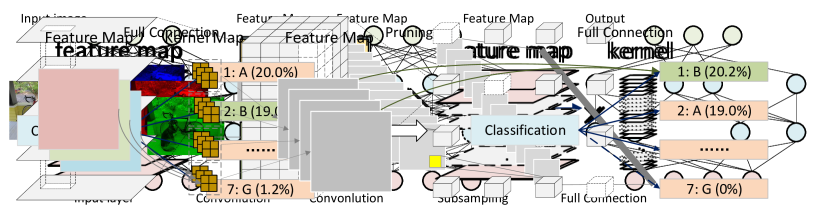
Figure 3: Dynamic Runtime Feature Map Pruning: Prune less contributed feature maps to reduce both data loading and computation resources usage by stopping minor feature maps and corresponding kernel maps goes into computation units

Even with memory performance improvements, bandwidth is still a limiting factor in many neural network designs Rhu2018 . When direct connection to memory is not possible, common bus protocols such as PCIe further limit the peak available bandwidth within a system. Once a system is fixed, further performance improvements may only be achieved by reducing the bandwidth requirements of the networks being implemented. One way of achieving this is by reducing the number of feature maps being loaded.

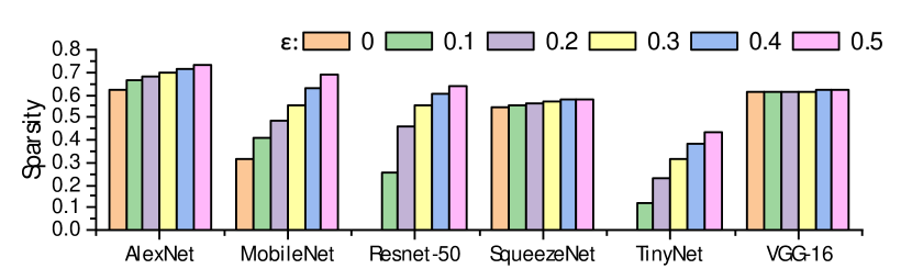
Figure 4: Feature Map Value Sparsity in Convolutional Layers: The x-axis identifies a number of popular CNNs with each bar being the value of coefficients at or within an epsilon of 0. The y-axis gives the proportion of coefficients within that epsilon.

Figure 4 shows the feature map sparsity of some common neural networks. Only convolutional layers are considered (i.e. fully connected layers are not included). The baseline measure of sparsity is 0-valued feature map elements as represented by the orange bar. As an example, AlexNet has over 60% of feature map with 0 values while ResNet and TinyNet don’t have any 0-valued feature map element. It also shows that for values within an epsilon of 0, some networks have many more elements that can be pruned (e.g. MobileNet and TinyNet) while other networks have much smaller variance (e.g. VGG16).

We also did statistics for all parameters (every single value in trained model) and convolutional coefficients (kernel map) in table 1 and table 2. Basically they are similar except VGG and AlexNet who has heavy number of parameter for connected coefficients. In our experiments, we prune the minor valued kernel map coefficients (both in convolutional layer and connected layer, biases not included) without any fine tune, then valid with 100 images of ImageNet dataset, the result is showing with three colors in table 1, Green means both Top-1 and Top-5 drop less than 1%, Yellow indicates one of them (mostly Top-1) drop more than 1%, Red means both of Top-1 and Top-5 drop more than 1%.

Table 1: All Parameter Sparsity

Parameter Sparsity	0.000	0.005	0.010	0.020	0.040	0.060	0.080	0.100	0.200
AlexNet	0.00%	71.29%	92.15%	98.34%	99.74%	99.91%	99.95%	99.97%	99.99%
MobileNet	0.00%	9.02%	12.56%	19.24%	31.99%	43.84%	54.47%	63.76%	90.12%
ResNet50	0.00%	61.86%	86.83%	97.29%	99.39%	99.64%	99.72%	99.74%	99.78%
SqueezeNet	0.00%	9.18%	18.17%	35.14%	62.84%	80.38%	89.82%	94.52%	99.35%
TinyNet	0.00%	19.71%	37.70%	64.25%	86.39%	93.05%	95.91%	97.36%	98.95%
VGG16	0.00%	87.29%	96.68%	99.54%	99.94%	99.97%	99.99%	99.99%	99.99%

Table 2: Convolution Kernel Sparsity

Kernel Sparsity	0.000	0.005	0.010	0.020	0.040	0.060	0.080	0.100	0.200
AlexNet	0.00%	29.97%	52.66%	80.34%	95.98%	98.60%	99.32%	99.61%	99.94%
MobileNet	0.00%	8.85%	12.39%	19.11%	32.00%	44.01%	54.80%	64.23%	90.95%
ResNet50	0.00%	62.03%	87.09%	97.57%	99.65%	99.89%	99.96%	99.98%	100.0%
SqueezeNet	0.00%	9.15%	18.12%	35.07%	62.79%	80.36%	89.81%	94.52%	99.35%
TinyNet	0.00%	19.90%	38.05%	64.85%	87.19%	93.89%	96.78%	98.22%	99.80%
VGG16	0.00%	47.48%	77.77%	96.17%	99.49%	99.83%	99.93%	99.96%	99.99%

Most current techniques only prune kernel maps. Our technique proposes not to remove entire kernels but only specific feature maps that do not contribute to the effectiveness of the network. This is done dynamically at runtime and has the advantage of reducing the number of feature maps loaded (i.e. bandwidth) without limiting the type of network architecture that can be pruned.

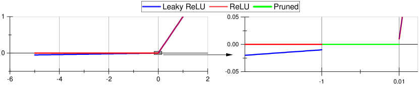
Figure 5: Left: ReLU and Leaky ReLU activation function layout, Right: prune with $|\epsilon|=0.01$ layout

Figure 5 shows activation functions for ReLU and leaky ReLU. ReLU has the property that for all values of $x\leq 0$ the function remains 0 (e.g. $f(x\leq 0)=0$). Leaky ReLU and some other similar activation functions do not have this property and allow small negative values of $x$ so as to smooth gradients during training Maas2013 . A result of this is that they have many less 0-valued parameters. ResNet and TinyNet both use leaky ReLU and as shown in Figure 4 they both have low 0-sparsity. However, in some cases, while not exactly zero, the values may be close to 0.

$$active(x)=\begin{cases}x&\mbox{ $\epsilon<x$}\\ 0&\mbox{-0.01 $\epsilon\leq x\leq\epsilon$}\\ 0.01\times x&\mbox{$x<-0.01\epsilon$}\end{cases}$$ (1)

Equation 1 shows the activation function we compute for feature maps with epsilon pruning. For any value of epsilon greater than $x$ the function returns $x$. For positive values of $x$ that are less than epsilon the function returns 0 and effectively is pruned. To accommodate leaky ReLU we multiply negative values of $x$ by a small coefficient to transform it to a positive value that is likely to be pruned.

Algorithm 1: Dynamic Feature Map Pruning

Input: channel size, including height, width, number (H, W, C).

capability of processor, max width and height to process (h, w).

Output: marker for small data filled channels.

we define the column “part + 1” as the zero mark of each channel.

for each i in C

// get the channel pieces number

channel_part = ceil ( W $\times$ H / w $\times$ h)

// check if all zero in one part

for all j in channel_part

for all k in w $\times$ h

if ( abs(value[k] < $\epsilon$ )

channel_zero_mark[i][j]=1

end if

end for

// check if all zero in one channel

channel_zero_mark[i][channel_part + 1] = sum (channel_zero_mark[i][0 : channel_part])

end for

end for

Algorithm 1 describes a brute-force naive technique for dynamic feature map pruning. It is applied after activation function of Equation 1 is applied. For all feature map channels in a convolutional neural network we look at the element values. If we determine that a feature map has 0-valued coefficients such that the entire channel is unused, we mark it and subsequently do not compute any values for that feature map. Specifically, we count the number of zeros (or absolute value less than $\epsilon$). If the entire channel is filled with values less than $\epsilon$ we then regard this channel as a zero channel and mark it for later identification. When loading a feature map for processing, if the channel was marked to be within an $\epsilon$ of 0, we will prune it. Some implementations may not implement sufficient neurons (multiply-accumulate units) to process an entire feature map simultaneously. In this case we will break the feature map into smaller pieces. We then sum the flag of each part to determine if the entire feature map is filled with $\epsilon$ zero elements. If so, the entire feature map will be marked as zero-filled and will be skipped thus saving feature map loading and reducing bandwidth requirements. Our source code for our technique is available at Github.

3 Experimental Results

3.1 Classification Accuracy

We implemented our dynamic pruning algorithm using Darknet - a C language deep neural network framework darknet13 . We compute statistics by counting the number of feature maps loaded, noting that if a computation unit has a small cache, a feature map will be loaded more than once. In this work we don’t consider this additional effect.

Table 3: Accuracy performance of different $\epsilon$ pruning

	Top-1 Accuracy						Top-5 Accuracy
Epsilon	0.0	0.1	0.2	0.3	0.4	0.5	0.0	0.1	0.2	0.3	0.4	0.5
AlexNet	57.17%	-0.01%	0.01%	0.07%	0.12%	0.14%	80.20%	-0.01%	0.00%	0.02%	0.03%	0.08%
MobileNet	71.44%	-0.02%	0.02%	0.74%	3.97%	24.64%	90.35%	0.01%	0.06%	0.49%	2.46%	19.91%
ResNet-50	75.83%	0.02%	0.06%	1.13%	5.56%	12.22%	92.89%	0.00%	0.03%	0.68%	3.26%	7.81%
SqueezeNet	57.13%	0.00%	0.00%	0.00%	0.00%	0.00%	80.13%	0.00%	0.00%	0.00%	0.00%	0.00%
TinyNet	58.71%	0.00%	0.01%	0.07%	1.28%	6.96%	81.73%	0.00%	0.00%	0.04%	0.90%	5.99%
VGG-16	70.39%	0.00%	0.00%	0.00%	0.00%	0.00%	89.79%	0.00%	0.00%	0.00%	0.00%	0.00%

To validate our technique we used the ILSVRC2012-50K image dataset containing 1000 classes Russakovsky2015 . Table 3 lists our results based on the 50,000 images using GPU acceleration.

Our results show that using an $\epsilon=0.1$ for pruning has no significant loss in accuracy for the top-1 while reducing feature map loading up to 10%. At $\epsilon=0.2$, top-1 accuracy drooped but top-5 accuracy is still state-of-the-art performance. We note that not all networks improved using this approach. We comment on that in Section 5. The results show that layers using ReLU activation have the most feature maps removed and therefore the highest feature map loading reduction. Leaky ReLU with an $\epsilon=0.0$ has little advantage as its feature maps do not have many 0-values.

Table 4: Accuracy of Networks And Number of Feature Maps Pruned

	without pruning					$\epsilon=0.1$ pruning					saved fmap load
net	cat	dog	eagle	giraffe	horse	cat	dog	eagle	giraffe	horse	saved (avg saved/no prune)
AlexNet	40.35%	19.03%	79.03%	36.50%	53.13%	40.34%	19.12%	79.15%	36.47%	53.23%	5.51%	(43k/781k)
MobileNet	24.64%	28.51%	91.43%	27.40%	29.35%	28.56%	29.59%	92.02%	28.00%	28.03%	10.16%	(940k/9255k)
ResNet-50	23.77%	95.19%	68.11%	76.37%	20.94%	19.84%	94.89%	68.06%	73.38%	20.63%	1.60%	(323k/20086k)
SqueezeNet	92.67%	57.34%	58.60%	45.58%	93.17%	92.67%	57.34%	58.60%	45.58%	93.17%	0.56%	(18k/3290k)
TinyNet	15.25%	14.51%	54.11%	29.71%	25.59%	15.25%	14.51%	54.11%	29.71%	25.59%	0	(0/3458k)
VGG-16	26.79%	56.49%	92.12%	97.73%	39.04%	26.82%	56.55%	92.14%	97.73%	39.01%	0.32%	(50k/15087k)

Table 4 shows single image accuracy without pruning and pruning with $\epsilon=0.1$. We note that the labels are not changed (i.e. there is no prediction involved). We compare the ground truth labels with the effects exclusively related to pruning the network. In some cases the pruned network outperformed the unpruned. This is inline with other researcher’s results Yu2017 ; Huang2018a . The last column shows the number of feature maps pruned at $\epsilon=0.1$. For example, MobileNet reduced the number of feature maps loaded by 940 thousand out of a total number of 9255 thousand feature maps to be computed. This is approximated a 10% savings in the number of feature maps loaded. It should be noted that due to long simulation times Table 4 was determined using 5 random images. Therefore the results should be considered preliminary.

Additional results for MobileNet not shown in Table 4 reveals that MobileNet particularly benefited from feature map pruning. With $\epsilon=0$ pruning, MobileNet reduced 36/54 ReLU activated convolutional layers resulting in a feature map loading reduction of 7.8%. AlexNet reduced 3/5 ReLu activated convolutional layers reduced feature map loading of 5.1%, while SqueezeNet reduced 5/26 layers resulting in a 0.7% reduction. Other networks using leaky ReLU, as anticipated, do not have reduced feature map loading with $\epsilon=0$. Figure 6 shows the convolutional layer-by-layer feature map loading with and without dynamic pruning.

Among the networks we’ve tested, MobileNet and AlexNet (which both use ReLU) are much improved while Squeezenet (uses ReLU), VGG-16 (uses ReLU) and Resnet-50 (leaky and linear) are marginally if at all improved. Finally, Tinynet (leaky ReLU) is not improved at all.

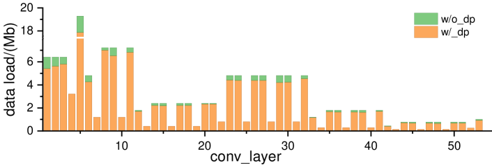
Figure 6: Dynamic Pruning Performance on MobileNet by Convolutional Layer

Figure 6 shows the feature loading requirements for MobileNet by convolution layer. The y-axis displays the Mega-bits of data required to be read. The x-axis displays the network layers. The stacked bars show the data requirements with and without dynamic pruning. $\epsilon=0$ is used and shows that dynamic pruning can reduce the image "dog", which shown in 1, data loading requirements by about 9.2% as averaged across all the layers. A few layers of MobileNet use linear activation functions and therefore don’t benefit from $\epsilon=0$ pruning.

We’ve also run AlexNet experiments on Caffe with and without static pruning. The results shows a similar runtime feature map sparsity of about 60%. Resulting 0.45% feature map loading reduction with channel-wise dynamic feature map pruning after static pruning is applied, the result for none static pruned is also minor as 0.79%.

Table 5: Top-1 Accuracy Loss Versus $epsilon$ Pruning Threshold

$\epsilon$	0.0		0.1		0.2		0.3		0.4		0.5
net	accuracy	reduce	loss	reduce	loss	reduce	loss	reduce	loss	reduce	loss	reduce
AlexNet	57.173%	5.064%	0.050%	5.885%	0.050%	6.552%	0.100%	7.951%	0.450%	9.174%	0.450%	10.066%
MobileNet	71.449%	7.796%	-0.250%	10.297%	-0.350%	10.863%	0.450%	11.338%	4.450%	12.268%	29.250%	14.386%
SqueezeNet	57.129%	0.707%	0.000%	0.703%	0.000%	0.714%	0.000%	0.716%	0.000%	0.717%	0.000%	0.718%

3.2 Balance Between Feature Map Loading Reduction and Accuracy

We characterized a range of $\epsilon$ values between 0 and 0.5 with a step size of 0.1 to determine if a feature map should be pruned. We evaluated the effect of $\epsilon$ on MobileNet, SqueezeNet, and TinyNet using 2000 images from ImageNet. The results show that as $\epsilon$ increases the accuracy decreases. Table 5 shows the accuracy loss with varying $\epsilon$.

4 Related Work

Bandwidth reduction is accomplished by reducing the loading of parameters or the number of bits used by the parameters. This lead to further research on sparsity, quantification, and weight sharing. Bandwidth reduction using reduced precision values has been previously proposed. Historically most networks are trained using 32-bit single precision floating point numbers Sze2017a . Ma Ma2016 and Kaiming Kaiming2015 have shown that 32-bit single precision parameters produced during training can be reduced to 8-bit integers for inference without significant loss of accuracy. Jacob Jacob2017 used 8-bit integers for both training and inference but with an accuracy loss of 1.5% on ResNet-50. Li Li and Leng Leng2017 showed that for ternary weight-only quantized networks the accuracy drop was as low as 2.57%. Zhou Zhoua2016 , and Hubara Hubara2016a took this to an extreme using only 1-bit binary weights, less than 4-bit activation functions, and 6-bit gradients with accuracy losses of 16.4%. Zhou expanding on his earlier work Zhou2017 and Das Das2018 improved the accuracy loss to between 0.49% to 2.28% using binary values for pre-trained networks and fine tuning the results. Our present work does not consider reduced precision parameters but may be incorporated into future research since it is complementary to our approach.

Compressing sparse parameter networks has been carried out to save both computation and bandwidth, Chen chen2015 describes using a hash algorithm to decide which weights can be shared. This focused only on fully connected layers and uses pre-trained weight binning rather than dynamically determining the bins during training. Han Han2015DeepCompression describes weight sharing combined with Huffman coding. Weight sharing is accomplished by using a k-means clustering algorithm instead of a hash algorithm to identify neurons that may share weights. This realized a pruned and quantized parameter storage reduction of $1.18\times$ to $1.58\times$. In our technique we don’t currently share weights but it is possible to combine our technique with weight sharing.

Studies by Foroosh and Glorot Foroosh2015 ; Glorot2011 have shown that in networks with many parameters a significant amount of the parameters have values of 0 or close to zero. Foroosh feeds the sparse maps into a sparse matrix multiplication algorithm which decomposes the maps into a sparse format to accelerate the computation. This technique shows an accuracy loss of less than 1%. Ren Ren2018 exploits this sparsity using low-resolution segmentation networks. They compute convolutions on a block-wise decomposition of the mask. This technique is used in an autonomous vehicle application where lidar scans are shown to have repetition and 0-valued numbers.

Han Han2016a further incorporates weight sharing and sparsity into his Efficient Inference Engine (EIE) Han2016 . The EIE is intended for fully connected layers where the shared and compressed (sparse pruned) nets are used for efficient inference. Lavin Lavin2015 further shows that a $3\times 3$ winograd convolution can reduce throughput for small filter sizes by $2.25\times$. EIE could support this kind of convolution by tuning the channel-wise convolution to matrix $\times$ vector operations.

Network pruning is an important component for both memory size and bandwidth usage. It also reduces the number of computations. Early research used large scale networks with static pruning to generate smaller networks to fit end-to-end applications without significant accuracy drop Bucilua2006 .

LeCun as far back as 1990 proposed to prune non-essential weights using the second derivative of the loss function LeCun . This static pruning technique reduced network parameters by a quarter. He also showed that the sparsity of DNNs can provide opportunities to accelerate network performance.

Han Han2015DeepCompression described a static method to prune kernel maps that don’t contribute to the classification. This technique uses re-training to optimize the neural network. They also specifically remove weights with small values in addition to feature map pruning. The pruning and retraining process was iterated 3 times for a $9\times$ reduction in total parameters. Han’s learning weights and connection work requires retraining. Guo Guo2016 describes a method using pruning and splicing that compressed AlexNet by factor of $7.7\times$. This significantly reduced the training iterations from 4800K to 700K. However this type of pruning results in an asymmetric network complicating hardware implementation.

Most network pruning methods typically prune the kernel rather than feature maps Guo2016 . In addition to significant retraining times, most of the weight compression is contributed by fully connected layers. AlexNet and VGG particularly have many parameters in fully connected layers. Convolutional layers by contrast realize only a 50% reduction on average Han2015DeepCompression . Our technique uses dynamic pruning of feature maps rather than weights and requires no retraining. We realize a 10.2% reduction in feature map loading without loss of accuracy and importantly we do not limit the type of networks that can be pruned.

Bolukbasi Bolukbasi2017AdaptiveNN has reported a system that can adaptively choose which layers to exit early. They format the inputs as a directed acyclic graph with various pre-trained network components. They evaluate this graph to determine leaf nodes where the layer can be exited early. This can be considered a type of dynamic layer pruning.

For instruction set processors, Feature maps or the number of filters used to identify objects is a large portion of bandwidth usage Sze2017 - especially for depth-wise or point-wise convolutions where feature map computations are a larger portion of the bandwidthChollet2017 . Lin Lin2017 used Runtime Neural Pruning (RNP) to pretrain a side network to predict which feature maps wouldn’t be needed. This is a type of dynamic runtime pruning. They found $2.3\times$ to $5.9\times$ acceleration with top-5 accuracy loss from 2.32% to 4.89%. However, in this way of pruning, the pre-trained supervision network still needs to load parameters to figure out which feature maps will be removed. In our approach an additional neural network to predict which feature maps may be ignored isn’t required. Instead, we look for feature maps that are not being used in the current classification. RNP, as a predictor, may need to be retrained for different classification tasks. The prediction network may also increase the original network size. Our technique doesn’t require additional neurons (or networks) to determine if a feature map will be useful to the current classification (e.g. it is not a prediction).

Rather, we look at all the feature maps and remove the maps that are dynamically determined not to be participating in the classification.

Rhu Rhu2018 recently described a compressing DMA engine (cDMA) that improved virtualized DNNs (vDNN) performance by 32%. It compresses activated feature maps using ReLU activation functions prior to transfer. The current implementation operates on elements and takes advantage of sparsity within a feature map without removing the entire channel. The technique uses a bitmap to record all non-zero/zero elements of a feature map. The information is then compressed for efficient transfer across a PCIe bus. Compressed sparse maps with a zero bitmap are then decompressed using a function similar to Caffee’s im2col Jia2014 . A disadvantage of this approach is that it spreads out the feature map making it difficult to map to computation units. Our technique prunes by channel rather than elements. This benefits instruction set processors, particularly signal processors, because data can be easily loaded into the processor using sliding windows.

5 Discussion and Future Work

In our experiment, we count feature map loading once as we assume the system has sufficient memory to hold all the feature map weights and data. For some networks (e.g. VGG-16) that may require 60MB just for the feature map weights. For processors with less capacity this will require the maps to be partially loaded. We plan to investigate this in future works.

From our experiments we conclude that for ReLU activated neural networks (e.g. AlexNet) static pruning can be effective since ReLU converts negative values to zeros leading to sparse networks. We did find minor improvements of <0.5% when applying dynamic pruning after static pruning with Caffe. However not all networks can be statically pruned (e.g. ResNet and TinyNet).

Figure 7 shows two CNN network architectures - one using traditional convolutional kernels (figure 7(a)) and one using depth-wise convolutional kernels (figure 7(b)). Modern CNNs tend to use depth-wise convolutional kernels due to reduced computational complexity Chollet2017 . A traditional convolutional layer for an $I$ input, $O$ output, $K$ kernel, $A$ area has $I\times K\times O\times A$ computations required. A depth-wise convolutional layer requires only $I\times K\times A$ computations, Depth-wise convolutional layers, in addition to requiring less computations, have the advantage that the feature map used only once to generate new ones thereby reducing feature map loading. Significantly, with the reduced kernel size, they also increase the ratio of feature maps to kernel maps (weight) by a factor of $O$. We expect this to be of benefit in dynamic feature map pruning. Point-wise convolutions have a similar benefit due to the reduction in weights.

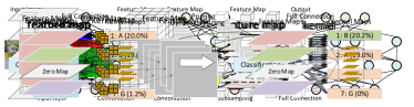
(a) Normal Convolution

(b) Depth-wise Convolution

Figure 7: Comparing Depth-wise Convolution with Normal Convolution

Table 5 shows that for some networks an $\epsilon=0.2$ feature map pruning had no loss of accuracy for top-1. As shown in figure 8, we believe that is because in the latter part of the network, part of the scattered weights have been transferred to the filter with the highest probability of predicting the correct classification. This is an area of future research.

Figure 8: Prune Increased Classification Accuracy: The pruning operation move a small prediction (class G) to a right class (class B) so that the classification result get corrected

As we introduced in Section 4, compression networks typically operate on kernel maps (weights). The more network weights that are statically pruned, the more bandwidth will be consumed by feature maps. Further, unless statically pruning removes an entire neuron, it can not reduce bandwidth usage since the zero feature maps will still be loaded. We have shown that even without weight optimizations, feature map bandwidth is comparable to weight bandwidth when depth-wise (or point-wise) convolutions are employed. Additionally, weight pruning tunes the ratio of weights to feature maps for each layer to balance accuracy and compression. This requires retraining each time a layer is pruned. As networks become deep with many layers, retraining after pruning each layer is computationally expensive.

As static pruning provides 50% or less contribution to convolutional layer weight compression, they don’t hurt the high runtime sparsity of up to 70%, with our pruning activation the feature map sparsity going up with minor or without loss of accuracy. The 10% all-zero feature map also provides additional opportunity of kernel map pruning.

In this work we have determined which feature maps to prune using a fixed $epsilon$. Our future work focuses on determining and possibly dynamically modifying these values by inspecting layer channels. This technique might also be useful during training.

Figure 9: Sparsity distribution of weights: Zeros may be distributed through feature maps (left), tensors (middle), or tensor arrays (right)

As we see in figure 4 some CNNs have 50+% sparsity. In such cases we found only 10% channel-wise reduction. We suspect that in a well trained classification model, among the large number of layers and channels, there should be specific maps that predict the final class. Our future work will look specifically at designing networks that take advantage of dynamic feature map pruning where few parameters are 0-valued but feature maps may dynamically be 0-valued. We suspect this may also be of benefit to capsule networks Sabour2017 .

6 Conclusion

In this paper, we analyzed feature map parameter sparsity of six different convolutional neural networks - AlexNet, MobileNet, ResNet-50, SqueezeNet, TinyNet, and VGG16. We found a range of sparsity from no sparsity to greater than 50% sparsity. When considering parameter values an $epsilon$ away from 0, all networks exhibited some level of sparsity. Of the networks considered, those using ReLU (AlexNet, SqueezeNet, VGG16) contain a high percentage of 0-valued parameters (50%+) and can be statically pruned. However static pruning can lead to irregular networks. Networks with Non-ReLU activation functions in some cases may not contain any 0-valued parameters (ResNet-50, TinyNet). Further static pruning on large networks that require retraining may not be computationally feasible when $epsilon$ values near 0 are considered.

We also investigated runtime feature map usage and found that input feature maps comprise the majority of bandwidth requirements when depth-wise convolution and point-wise convolutions used. Our approach uses dynamic runtime pruning of feature maps rather than parameters. This technique is complimentary to static pruning and doesn’t require retraining of the CNN. Using this technique we show that 10% of dynamic feature map execution can be removed without loss of accuracy. We then extend dynamic pruning to allow for values within an $epsilon$ of zero and show a further 5% reduction of feature map loading with a 1% loss of accuracy in top-1. We achieved a slight further reduction on networks that were able to be statically pruned. As depth-wise and point-wise convolutional kernels become more common, the amount of computations performed by feature maps will increase possibly further benefiting from dynamic pruning.

References

- [1] Yann Lecun, Yoshua Bengio, and Geoffrey Hinton. Deep learning, 2015.
- [2] Forrest N. Iandola, Song Han, Matthew W. Moskewicz, Khalid Ashraf, William J. Dally, and Kurt Keutzer. SqueezeNet: AlexNet-level accuracy with 50x fewer parameters and <0.5MB model size. arxiv.org, 2016.
- [3] Paulius Micikevicius, Sharan Narang, Jonah Alben, Gregory Diamos, Erich Elsen, David Garcia, Boris Ginsburg, Michael Houston, Oleksii Kuchaiev, Ganesh Venkatesh, and Hao Wu. Mixed Precision Training. In International Conference on Learning Representations, 10 2018.
- [4] Misha Denil, Babak Shakibi, Laurent Dinh, Marc’Aurelio Ranzato, and Nando de Freitas. Predicting Parameters in Deep Learning. In Advances in neural information processing systems., pages 2148–2156, 6 2013.
- [5] Yiwen Guo, Anbang Yao, and Yurong Chen. Dynamic Network Surgery for Efficient DNNs. In Advances in Neural Information Processing Systems 29, pages 1379–1387, 2016.
- [6] Song Han, Huizi Mao, and William J. Dally. Deep Compression: Compressing Deep Neural Networks with Pruning, Trained Quantization and Huffman Coding. arXiv preprint arXiv:1510.00149, 45(4):199–203, 10 2015.
- [7] Ruichi Yu, Ang Li, Chun-Fu Chen, Jui-Hsin Lai, Vlad I. Morariu, Xintong Han, Mingfei Gao, Ching-Yung Lin, and Larry S. Davis. NISP: Pruning Networks using Neuron Importance Score Propagation. arXiv:1711.05908, 11 2017.
- [8] Ji Lin, Yongming Rao, Jiwen Lu, and Jie Zhou. Runtime Neural Pruning. In 31st Conference on Neural Information Processing Systems (NIPS 2017), pages 2178–2188, 2017.
- [9] Hassan Foroosh, Marshall Tappen, and Marianna Penksy. Sparse Convolutional Neural Networks. 2015 IEEE Conference on Computer Vision and Pattern Recognition (CVPR), pages 806–814, 2015.
- [10] Song Han, Jeff Pool, John Tran, and William J. Dally. Learning both Weights and Connections for Efficient Neural Networks. Lancet (London, England), 346(8988):1500, 6 2015.
- [11] Y. LeCun, B. Boser, J. S. Denker, D. Henderson, R. E. Howard, W. Hubbard, and L. D. Jackel. Backpropagation Applied to Handwritten Zip Code Recognition. Neural Computation, 1(4):541–551, 12 1989.
- [12] Minsoo Rhu, Mike O’Connor, Niladrish Chatterjee, Jeff Pool, Youngeun Kwon, and Stephen W. Keckler. Compressing DMA Engine: Leveraging Activation Sparsity for Training Deep Neural Networks. Proceedings - International Symposium on High-Performance Computer Architecture, 2018-Febru:78–91, 2018.
- [13] Andrew L. Maas, Awni Y. Hannun, and Andrew Y Ng. Rectifier nonlinearities improve neural network acoustic models. In ICML ’13, 2013.
- [14] Joseph Redmon. Darknet: Open Source Neural Networks in C, 2016.
- [15] Olga Russakovsky, Jia Deng, Hao Su, Jonathan Krause, Sanjeev Satheesh, Sean Ma, Zhiheng Huang, Andrej Karpathy, Aditya Khosla, Michael Bernstein, Alexander C. Berg, and Li Fei-Fei. ImageNet Large Scale Visual Recognition Challenge. International Journal of Computer Vision, 115(3):211–252, 12 2015.
- [16] Qiangui Huang, Kevin Zhou, Suya You, and Ulrich Neumann. Learning to prune filters in convolutional neural networks. In Proceedings - 2018 IEEE Winter Conference on Applications of Computer Vision, WACV 2018, volume 2018-Janua, pages 709–718, 1 2018.
- [17] Vivienne Sze, Yu-Hsin Chen, Tien-Ju Yang, and Joel S. Emer. Efficient Processing of Deep Neural Networks: A Tutorial and Survey. Proceedings of the IEEE, 105(12):2295–2329, 12 2017.
- [18] Yufei Ma, Naveen Suda, Yu Cao, Jae Sun Seo, and Sarma Vrudhula. Scalable and modularized RTL compilation of Convolutional Neural Networks onto FPGA. FPL 2016 - 26th International Conference on Field-Programmable Logic and Applications, 2016.
- [19] Kaiming He, Xiangyu Zhang, Shaoqing Ren, and Jian Sun. Deep Residual Learning for Image Recognition. Arxiv.Org, 7(3):171–180, 12 2015.
- [20] Benoit Jacob, Skirmantas Kligys, Bo Chen, Menglong Zhu, Matthew Tang, Andrew Howard, Hartwig Adam, and Dmitry Kalenichenko. Quantization and Training of Neural Networks for Efficient Integer-Arithmetic-Only Inference. CoRR, abs/1712.0, 12 2017.
- [21] Fengfu Li, Bo Zhang, and Bin Liu. Ternary Weight Networks. In 30th Conference on Neural Information Processing Systems (NIPS 2016), 2016.
- [22] Cong Leng, Hao Li, Shenghuo Zhu, and Rong Jin. Extremely Low Bit Neural Network: Squeeze the Last Bit Out with ADMM. CoRR, abs/1707.0, 7 2017.
- [23] Shuchang Zhou, Yuxin Wu, Zekun Ni, Xinyu Zhou, He Wen, and Yuheng Zou. DoReFa-Net: Training Low Bitwidth Convolutional Neural Networks with Low Bitwidth Gradients. CoRR, abs/1606.0(1):1–13, 6 2016.
- [24] Itay Hubara, Matthieu Courbariaux, Daniel Soudry, Ran El-Yaniv, and Yoshua Bengio. Quantized Neural Networks: Training Neural Networks with Low Precision Weights and Activations. Journal of Machine Learning Research, 18:187–1, 2017.
- [25] Aojun Zhou, Anbang Yao, Yiwen Guo, Lin Xu, and Yurong Chen. Incremental Network Quantization: Towards Lossless Cnns With Low-Precision Weights. arXiv preprint arXiv:1702.03044, 2017.
- [26] Dipankar Das, Naveen Mellempudi, Dheevatsa Mudigere, Dhiraj Kalamkar, Sasikanth Avancha, Kunal Banerjee, Srinivas Sridharan, Karthik Vaidyanathan, Bharat Kaul, Evangelos Georganas, Alexander Heinecke, Pradeep Dubey, Jesus Corbal, Nikita Shustrov, Roma Dubtsov, Evarist Fomenko, and Vadim Pirogov. Mixed Precision Training of Convolutional Neural Networks using Integer Operations. CoRR, abs/1802.0:1–11, 2 2018.
- [27] W. Chen, J. Wilson, S. Tyree, K. Weinberger, and Y. Chen. Compressing neural networks with the hashing trick. In In International Conference on Machine Learning, pages 2285–2294, 2015.
- [28] Xavier Glorot, Antoine Bordes, and Yoshua Bengio. Deep sparse rectifier neural networks. AISTATS ’11: Proceedings of the 14th International Conference on Artificial Intelligence and Statistics, 15:315–323, 2011.
- [29] Mengye Ren, Andrei Pokrovsky, Bin Yang, and Raquel Urtasun. SBNet: Sparse Blocks Network for Fast Inference. In Proceedings of the IEEE Conference on Computer Vision and Pattern Recognition (CVPR), pages 8711–8720, 1 2018.
- [30] Song Han, Junlong Kang, Huizi Mao, Yiming Hu, Xin Li, Yubin Li, Dongliang Xie, Hong Luo, Song Yao, Yu Wang, Huazhong Yang, and William J. Dally. ESE: Efficient Speech Recognition Engine with Sparse LSTM on FPGA. Proceedings of the 2017 ACM/SIGDA International Symposium on Field-Programmable Gate Arrays - FPGA ’17, pages 75–84, 12 2016.
- [31] Song Han, Xingyu Liu, Huizi Mao, Jing Pu, Ardavan Pedram, Mark A. Horowitz, and William J. Dally. EIE: Efficient Inference Engine on Compressed Deep Neural Network. In 2016 ACM/IEEE 43rd Annual International Symposium on Computer Architecture (ISCA), volume 16, pages 243–254. IEEE, 6 2016.
- [32] Andrew Lavin and Scott Gray. Fast Algorithms for Convolutional Neural Networks. ISOCC 2016 - International SoC Design Conference: Smart SoC for Intelligent Things, pages 333–334, 9 2015.
- [33] Cristian Buciluǎ, Rich Caruana, and Alexandru Niculescu-Mizil. Model compression. In Proceedings of the 12th ACM SIGKDD international conference on Knowledge discovery and data mining - KDD ’06, page 535, New York, New York, USA, 2006. ACM Press.
- [34] Yann Le Cun, John S Denker, and Sara A Solla. Optimal Brain Damage. In Advances in Neural Information Processing Systems 2, volume 2, pages 598–605, 1990.
- [35] T Bolukbasi, J Wang, O Dekel, and V Saligrama. Adaptive Neural Networks for Efficient. In Thirty-fourth International Conference on Machine Learning, 2 2017.
- [36] Vivienne Sze, Vivienne Sze, Senior Member, Yu-hsin Chen, Student Member, and Tien-ju Yang. Efficient Processing of Deep Neural Networks : A Tutorial and Survey Efficient Processing of Deep Neural Networks : A Tutorial and Survey. Proceedings of the IEE, 105(April):2295–2329, 2017.
- [37] Francois Chollet. Xception: Deep Learning with Depthwise Separable Convolutions. In 2017 IEEE Conference on Computer Vision and Pattern Recognition (CVPR), volume 7, pages 1800–1807. IEEE, 7 2017.
- [38] Yangqing Jia, Evan Shelhamer, Jeff Donahue, Sergey Karayev, Jonathan Long, Ross Girshick, Sergio Guadarrama, and Trevor Darrell. Caffe: Convolutional Architecture for Fast Feature Embedding. CEUR Workshop Proceedings, 1436, 6 2014.
- [39] Sara Sabour, C V Nov, and Geoffrey E Hinton. Dynamic Routing Between Capsules. In Advances In Neural Information Processing Systems, pages 3856–3866, 2017.