Information geometric duality of $\phi$-deformed exponential families

Abstract

In the world of generalized entropies—which, for example, play a role in physical systems with sub- and super-exponential phasespace growth per degree of freedom—there are two ways for implementing constraints in the maximum entropy principle: linear- and escort constraints. Both appear naturally in different contexts. Linear constraints appear e.g. in physical systems, when additional information about the system is available through higher moments. Escort distributions appear naturally in the context of multifractals and information geometry. It was shown recently that there exists a fundamental duality that relates both approaches on the basis of the corresponding deformed logarithms (deformed-log duality). Here we show that there exists another duality that arises in the context of information geometry, relating the Fisher information of $\phi$-deformed exponential families that correspond to linear constraints (as studied by J. Naudts), with those that are based on escort constraints (as studied by S.-I. Amari). We explicitly demonstrate this information geometric duality for the case of $(c,d)$-entropy that covers all situations that are compatible with the first three Shannon-Khinchin axioms, and that include Shannon, Tsallis, Anteneodo-Plastino entropy, and many more as special cases. Finally, we discuss the relation between the deformed-log duality and the information geometric duality, and mention that the escort distributions arising in the two dualities are generally different and only coincide for the case of the Tsallis deformation.

I Introduction

Entropy is one word for several distinct concepts tmh17 . It was originally introduced in thermodynamics, then in statistical physics, information theory, and last in the context of statistical inference. One important application of entropy in statistical physics, and in statistical inference in general, is the maximum entropy principle, which allows us to estimate probability distribution functions from limited information sources, i.e. from data jaynes57 ; harremoes01 . The formal concept of entropy was generalized to also account for power laws that occur frequently in complex systems tsallis88 . Literally dozens of generalized entropies were proposed in various contexts, such as relativity kaniadakis02 , multifractals jizba04 , or black holes tsallis13 ; see thk-book for an overview. All generalized entropies, whenever they fulfil the first three Shannon-Khinchin axioms (and violate the composition axiom) are special cases of the $(c,d)$-entropy asymptotically ht11a . Generalized entropies play a role for non-multinomial, sub-additive systems (whose phasespace volume grows sub-exponentially with the degrees of freedom) tsallis05 ; ht11b , and for systems, whose phasespace grows super-exponentially jensen18 . All generalized entropies, for sub-, and super-exponential systems, can be treated within a single, unifying framework korbel18 .

With the advent of generalized entropies, depending on context, two types of constraint are used in the maximum entropy principle: traditional linear constraints (typically moments), $\langle E\rangle=\sum_{i}p_{i}E_{i}$, motivated by physical measurements, and the so-called escort constraints, $\langle E\rangle_{u}=\sum_{i}u(p_{i})E_{i}/\sum_{i}u(p_{i})$, where $u$ is some nonlinear function. Originally, the later were introduced with multifractals in mind tsallis88 . Different types of constraint arise from different applications of relative entropy. While for physics-related contexts (such as thermodynamics) linear constraints are normally used, in other applications, such as non-linear dynamical systems or information geometry it might be more natural to consider escort constraints. The question about their correct use and the appropriate form of constraints has caused a heated debate in the past decade tsallis98 ; abe03 ; htt09 ; htt09a ; ohara10 ; bercher12 . To introduce escort distributions in the maximum entropy principle in a consistent way, two approaches have been discussed. The first tsallis03 appears in the context of deformed entropies that are motivated by superstatistics beck03 . It was later observed in htg12 that this approach is linked to other deformed entropies with linear constraints through a fundamental duality (deformed-log duality), such that both entropies lead to the same functional form of MaxEnt distributions. The second way to obtain escort distributions was studied by Amari et al., and is motivated by information geometry and the theory of statistical estimation amari10 ; amari12 . There, escort distributions represent natural coordinates on a statistical manifold amari12 ; ay17 .

In this paper, we show that there exists an another duality relation between this information geometric approach with escort distributions, and an approach that uses linear constraints. The relation can be given a precise information geometric meaning on the basis of the Fisher information. We show this in the framework of $\phi$-deformations naudts02 ; naudts04 ; naudts11 . We establish the duality relation for both cases in the relevant information geometric quantities. As an example, we explicitly show the duality relation for the class of $(c,d)$-exponentials, introduced in ht11a ; ht11b . Finally, we discuss the relation between the deformed-log duality and the information geometric duality, and show that these have fundamental differences. Each type of duality is suitable for different applications.

Let us start with reviewing central concepts of (non-deformed) information geometry, in particular relative entropy and its relation to the exponential family through the maximum entropy principle. Relative entropy, or Kullback-Leibler divergence, is defined as

$$D_{KL}(\bm{p}\|\bm{q})=\sum_{i}p_{i}\log\left(p_{i}/q_{i}\right)\quad.$$ (1)

For the uniform distribution $\bm{q}=\bm{u}_{n}$ i.e, $q_{i}=1/n$, we have

$$D_{KL}(\bm{p}\|\bm{u}_{n})=\log n-S(\bm{p})\quad,$$ (2)

where $S(\bm{p})$ is Shannon entropy, $S(\bm{p})=-\sum_{i}p_{i}\log p_{i}$. It is maximized by the exponential family of distributions. Consider a normalization constraint, $\sum_{i}p_{i}=1$, and a set of constraints, $\sum_{j}p_{j}E_{ij}=\langle\bm{E}_{i}\rangle$. Further, consider a parametric family with parameter vector $\bm{\theta}\in\mathcal{M}$, where $\mathcal{M}$ is a parametric space. For simplicity, we use discrete probabilities. The family of probability distributions for configuration vector, $\bm{E}_{i}$, that maximizes Shannon entropy, can be written as

$$p_{i}(\bm{\theta})\equiv p(\bm{E}_{i};\bm{\theta})=\exp\left(\Psi(\bm{\theta})+\bm{\theta}\cdot\bm{E}_{i}\right)$$

$$=\exp\left(\Psi(\bm{\theta})+\sum_{j}\theta_{j}E_{ij}\right)\quad.$$ (3)

$\Psi(\bm{\theta})$ guarantees normalization. This family of distributions is called the exponential family. Fisher information defines the metric on the parametric manifold $\mathcal{M}$ by taking two infinitesimally separated points, $\bm{\theta}_{0}$, and $\bm{\theta}=\bm{\theta}_{0}+\delta\bm{\theta}$, and by expanding $D_{KL}(\bm{p}(\bm{\theta}_{0})\|\bm{p}(\bm{\theta}))$,

$$g^{F}_{ij}(\bm{\theta})=\left.\frac{\partial^{2}D_{KL}(\bm{p}(\bm{\theta}_{0})\|\bm{p}(\bm{\theta}))}{\partial\theta_{i}\partial\theta_{j}}\right|_{\bm{\theta}=\bm{\theta}_{0}}\quad.$$ (4)

Let us assume a probability simplex, $S^{n}$, with $n$ independent probabilities, $p_{i}$, and probability $p_{0}$. Its value is not independent, but determined by the normalization condition, $p_{0}=1-\sum_{i}p_{i}$. For the exponential family it is a well-known fact that Fisher information is equal to the inverse of the probability in Eq. (I)

$$g^{F}_{ij}(\bm{\theta})\equiv g^{F}_{ij}(\bm{p}(\bm{\theta}))=\frac{1}{p_{i}}\delta_{ij}+\frac{1}{p_{0}}\quad.$$ (5)

II Deformed exponential family

We briefly recall the definition of $\phi$-deformed logarithms and exponentials as introduced by Naudts naudts02 . The deformed logarithm is defined as

$$\log_{\phi}(x)=\int_{1}^{x}\mathrm{d}y\frac{1}{\phi(y)}\quad,$$ (6)

for some positive, strictly increasing function, $\phi(x)$, defined on $(0,+\infty)$. Then, $\log_{\phi}$ is an increasing, concave function with $\log_{\phi}(1)=0$. $\log_{\phi}(x)$ is negative on $(0,1)$, and positive on $(1,+\infty)$. Naturally, the derivative of $\log_{\phi}(x)$ is $1/\phi(x)$. The inverse function of $\log_{\phi}(x)$ exists; we denote it by $\exp_{\phi}(x)$. Finally, the $\phi$-exponential family of probability distributions is defined as a generalization of Eq. (I)

$$p_{i}(\bm{\theta})=\exp_{\phi}\left(\Psi(\bm{\theta})+\sum_{j}\theta_{j}E_{ij}\right)\quad.$$ (7)

We can express $\Psi(\bm{\theta})$ in the form

$$\Psi(\bm{\theta})=\log_{\phi}(p_{i}(\bm{\theta}))-\bm{\theta}\cdot\bm{E}_{i}\quad,$$ (8)

which allows us to introduce dual coordinates to $\bm{\theta}$. This is nothing but the Legendre transform of $\Psi(\bm{\theta})$, which is defined as

$$\varphi(\bm{\eta})=\bm{\eta}\cdot\bm{\theta}-\Psi(\bm{\theta})\quad,$$ (9)

where

$$\bm{\eta}=\nabla{\Psi(\theta)}\quad.$$ (10)

Because

$$\partial_{\theta_{j}}p_{i}(\bm{\theta})=\exp_{\phi}^{\prime}\left(\Psi(\bm{\theta})+\bm{\theta}\cdot\bm{E}_{i}\right)\left(\partial_{\theta_{j}}\Psi(\bm{\theta})+E_{ij}\right)$$ (11)

holds, and using $\sum_{i}\partial_{\theta_{j}}p_{i}(\bm{\theta})=0$, we obtain that

$$\bm{\eta}=\frac{\sum_{i}\exp_{\phi}^{\prime}(\Psi(\bm{\theta})+\bm{\theta}\cdot\bm{E}_{i})\cdot\bm{E}_{i}}{\sum_{i}\exp_{\phi}^{\prime}(\Psi(\bm{\theta})+\bm{\theta}\bm{E}_{i})}=\bm{E}_{i}\cdot\bm{P}^{\phi}\quad,$$ (12)

where $\bm{P}^{\phi}$ is the so-called escort distribution. With $\exp_{\phi}^{\prime}(\log_{\phi}(x))=\phi(x)$, the elements of $\bm{P}^{\phi}$ are given by

$$P^{\phi}_{j}=\frac{\phi(p_{j})}{\sum_{i}\phi(p_{i})}=\frac{\phi(p_{j})}{h_{\phi}(\bm{p})}\quad,$$ (13)

where we define $h_{\phi}(\bm{p})\equiv\sum_{i}\phi(p_{i})$. The Legendre transform provides a connection between the exponential family and the escort family, where the coordinates are obtained in the form of escort distributions. This generalizes the results for the ordinary exponential family, where the dual coordinates form a mixture family, which can be obtained as the superposition of the original distribution. The importance of dual coordinates in information geometry comes from the existence of a dually-flat geometry for the pair of coordinates. This means that there exist two affine connections with vanishing coefficients (Christoffel symbols). For the exponential family, the connection determined by the exponential distribution is called $e$-connection, and the dual connection leading to a mixture family that is called $m$-connection ay17 . For more details, see e.g. amari12 . We next look at generalizations of the Kullback-Leibler divergence and the Fisher information for the case of $\phi$-deformations.

III Deformed divergences, entropies, and metrics

For the $\phi$-deformed exponential family we have to define the proper generalizations of the relevant quantities, such as the entropy, divergence, and metric. A natural approach is to start with the deformed Kullback-Leibler divergence, denoted by $D_{\phi}(\bm{p}\|\bm{q})$. $\phi$-entropy can then be defined as

$$S_{\phi}(\bm{p})\sim-D_{\phi}(\bm{p}\|\bm{u}_{n})\quad,$$ (14)

where $\sim$ means that the relation holds up to a multiplicative constant depending only on $n$. Similarly, $\phi$-deformed Fisher information is

$$g_{\phi,ij}(\bm{\theta})=\left.\frac{\partial^{2}D_{\bm{\phi}}(p(\bm{\theta}_{0})\|p(\bm{\theta}))}{\partial\theta_{i}\partial\theta_{j}}\,\right|_{\bm{\theta}=\bm{\theta}_{0}}\quad.$$ (15)

There is now more than one way to generalize the Kullback-Leibler divergence. The first is Csiszár’s divergence Csiszar91

$$I_{f}(\bm{p}\|\bm{q})=\sum_{i}q_{i}f(p_{i}/q_{i})\quad,$$ (16)

where $f$ is a convex function. For $f(x)=x\ln x$, we obtain the Kullback-Leibler divergence. Note however, that the related information geometry based on the generalized Fisher information is trivial, because we have

$$g^{f}_{ij}(\bm{p})=f^{\prime\prime}(1)g_{ij}^{F}(\bm{p})\quad,$$ (17)

i.e., the rescaled Fisher information metric; see naudts04 . The second possibility is to use the divergence of Bregman type, usually defined as

$$D_{f}(\bm{p}\|\bm{q})=f(\bm{p})-f(\bm{q})-\langle\nabla f(\bm{q}),\bm{p}-\bm{q}\rangle\quad.$$ (18)

It can be understood as the first-order Taylor expansion of $f$ around $\bm{q}$, evaluated at $\bm{p}$. Let us next discuss two possible types of the Bregman divergence, which naturally correspond to the $\phi$-deformed family. For both, the $\phi$-exponential family is obtained from the maximum entropy principle of the corresponding $\phi$-entropy, however, under different constraints. Note that the maximum entropy principle is just a special version of the more general minimal relative entropy principle, which minimizes the divergence functional $D(\bm{p}\|\bm{q})$ w.r.t. $\bm{p}$, for some given prior distribution $\bm{q}$.

III.1 Linear constraints: divergence a là Naudts

One generalization of Kullback-Leibler divergence was introduced by Naudts naudts02 by considering $f(\bm{p})=\sum_{i}\left(\int_{1}^{p_{i}}\log_{\phi}(x)\mathrm{d}x+(1-p_{i})\right)$, which leads to

$$D^{N}_{\phi}(\bm{p}\|\bm{q})=\sum_{j}\int_{q_{j}}^{p_{j}}\mathrm{d}x\left(\log_{\phi}(x)-\log_{\phi}(q_{j})\right)\quad.$$ (19)

The corresponding entropy can be expressed as

$$S^{N}_{\phi}(\bm{p})=-\sum_{j}\int_{0}^{p_{j}}\mathrm{d}x\ln_{\phi}(x)\quad.$$ (20)

$S^{N}_{\phi}(\bm{p})$ is maximized by the $\phi$-exponential family under linear constraints. The Lagrange functional is

$$\mathcal{L}_{\phi}(\bm{p})=S^{N}_{\phi}(\bm{p})-\Psi\sum_{i}p_{i}-\sum_{j}\theta_{j}\sum_{i}p_{i}E_{ij}\quad,$$ (21)

which leads to

$$-\log_{\phi}(p_{i})-\Psi-\sum_{j}\theta_{j}E_{ij}=0\quad,$$ (22)

and we get

$$\Psi(\bm{\theta}) = -\sum_{i}p_{i}\log_{\phi}(p_{i})-\sum_{j}\theta_{j}\langle E_{j}\rangle$$ (23)

$$= -\langle\log_{\phi}(\bm{p})\rangle-\sum_{j}\theta_{j}\langle E_{j}\rangle\quad,$$

which is just Eq. (8), averaged over the distribution $p_{i}$. Note that Eq. (23) provides the connection to thermodynamics, because $\Psi(\theta)$ is a so-called Massieu function. For a canonical ensemble, i.e., one constraint on the average energy, $\theta$, plays the role of an inverse temperature, and $\Psi$ can be related to the free energy, $F(\theta)=\theta\Psi(\theta)$. Thus, the term $\langle\log_{\phi}(\bm{p})\rangle$ can be interpreted as the thermodynamic entropy, which is determined from Eq. (23). This is a consequence of the Legendre structure of thermodynamics.

The corresponding MaxEnt distribution can be written in the form

$$p_{i}(\bm{\theta}) = \exp_{\phi}\left(-\langle\log_{\phi}(\bm{p})\rangle-\sum_{j}\theta_{j}\left(\langle E_{j}\rangle-E_{ij}\right)\right)$$ (24)

$$= \exp_{\phi}\left(\Psi(\bm{\theta})+\bm{\theta}\cdot\bm{E}_{i}\right)\quad.$$

Finally, Fisher information metric can be obtained in the following form

$$g^{N}_{\phi,ij}(\bm{p})=\log_{\phi}^{\prime}(p_{i})\delta_{ij}+\log_{\phi}^{\prime}(p_{0})=\frac{1}{\phi(p_{i})}\delta_{ij}+\frac{1}{\phi(p_{0})}\quad.$$ (25)

III.2 Escort constraints: divergence a là Amari

Amari et al. amari10 ; amari12 use a different divergence introduced in vigelis13 , which is based on the choice, $f(\bm{p})=\sum_{i}P_{i}^{\theta}\log_{\phi}(p_{i})$. This choice is motivated by the fact that the corresponding entropy is just the dual function of $\Psi(\bm{\theta})$, i.e., $\varphi(\bm{\eta})$. This is easy to show, because

$$\varphi(\bm{\eta}) = \bm{\eta}\cdot\bm{\theta}-\Psi(\bm{\theta})=\sum_{j}P_{j}^{\phi}(\theta_{j}E_{ij}-\Psi(\bm{\theta}))$$ (26)

$$= \sum_{j}P_{j}^{\phi}\log_{\phi}(p_{j})\quad.$$

Thus, the divergence becomes

$$D^{A}_{\phi}(\bm{p}\|\bm{q})=\frac{1}{h_{\phi}(\bm{p})}\sum_{j}\phi(p_{j})(\log_{\phi}(p_{j})-\log_{\phi}(q_{j}))\quad,$$ (27)

and the corresponding entropy can be expressed from Eq. (26) as

$$S^{A}_{\phi}(\bm{p})=-\frac{1}{h_{\phi}(\bm{p})}\sum_{j}\phi(p_{j})\log_{\phi}(p_{j})\quad,$$ (28)

so it is a dual function of $\Psi(\bm{\theta})$. For this reason, the entropy is called canonical, because it is obtained by the Legendre transform from the Massieu function $\Psi$. Interestingly, the entropy is maximized by the $\phi$-exponential family under escort constraints. The Lagrange function is

$$\mathcal{L}_{\phi}(\bm{p})=\mathcal{S}^{A}_{\phi}(\bm{p})-\Psi\sum_{i}p_{i}-\sum_{j}\theta_{j}\sum_{i}P_{i}^{\phi}E_{ij}\quad.$$ (29)

After a straightforward calculation we get

$$\Psi(\bm{\theta})=-\sum_{i}\phi(p_{i}(\bm{\theta}))\quad,$$ (30)

and the corresponding MaxEnt distribution can be expressed as

$$p_{i}(\bm{\theta}) = \exp_{\phi}\left(-\langle\log_{\phi}(\bm{p})\rangle_{\phi}-\sum_{j}\theta_{j}\left(\langle E_{j}\rangle_{\phi}-E_{ij}\right)\right)$$ (31)

$$= \exp_{\phi}\left(\Psi(\bm{\theta})+\bm{\theta}\cdot\bm{E}_{i}\right)\quad,$$

where

$$\Psi(\bm{\theta})=-\langle\log_{\phi}(\bm{p})\rangle_{\phi}-\sum_{j}\theta_{j}\langle E_{j}\rangle_{\phi}\quad.$$ (32)

Here $\langle\cdot\rangle_{\phi}$ denotes the average under the escort probability measure, $\bm{P}^{\phi}$. Interestingly, in the escort constraints scenario, the “MaxEnt” entropy is the same as the “thermodynamic” entropy in the case of linear constraints. We call this entropy, $S^{A}_{\phi}(\bm{p})$, the dual entropy. Finally, one obtains the corresponding metric

$$g^{A}_{\phi,ij}(\bm{p}) = -\frac{1}{h_{\phi}(\bm{p})}\left(\frac{\log_{\phi}^{\prime\prime}(p_{i})}{\log_{\phi}^{\prime}(p_{i})}\delta_{ij}+\frac{\log_{\phi}^{\prime\prime}(p_{0})}{\log_{\phi}^{\prime}(p_{0})}\right)$$ (33)

$$= \frac{1}{h_{\phi}(\bm{p})}\left(\frac{\phi^{\prime}(p_{j})}{\phi(p_{j})}\delta_{ij}+\frac{\phi^{\prime}(p_{0})}{\phi(p_{0})}\right)\quad.$$

Note that the metric can be obtained from $\Psi(\bm{\theta})$ as $g^{A}_{\phi,ij}(\bm{\theta})=\frac{\partial^{2}\Psi(\bm{\theta})}{\partial\theta_{i}\partial\theta_{j}}$, which is the consequence of the Legendre structure of escort coordinates amari12 . For a summary for the $\phi$-deformed divergence, entropy and metric, see Table 1.

	$\phi$-deformation	linear constraints	escort constraints
divergence	$D_{\phi}(\bm{p}\|\bm{q})$	$\sum_{j}\int_{q_{j}}^{p_{j}}\mathrm{d}x\left(\log_{\phi}(x)-\log_{\phi}(q_{j})\right)$	$\frac{\sum_{j}\phi(p_{j})(\log_{\phi}(p_{j})-\log_{\phi}(q_{j}))}{\sum_{k}\phi(p_{k})}$
entropy	$S_{\phi}(\bm{p})$	$-\sum_{i}\int_{0}^{p_{i}}\log_{\phi}(x)\mathrm{d}x$	$-\sum_{i}\phi(p_{i})\log_{\phi}(p_{i})/\sum_{k}\phi(p_{k})$
metric	$g^{\phi}_{ij}(\bm{p})$	$\frac{1}{\phi(p_{i})}\delta_{ij}+\frac{1}{\phi(p_{0})}$	$\frac{1}{\sum_{k}\phi(p_{k})}\left(\frac{\phi^{\prime}(p_{i})}{\phi(p_{i})}\delta_{ij}+\frac{\phi^{\prime}(p_{0})}{\phi(p_{0})}\right)$

Table 1: $\phi$-deformation of divergence, entropy and Fisher information corresponding to $\phi$-exponential family under linear and escort constraints. For the ordinary logarithm, $\phi(x)=x$, the two entropies become Shannon entropy, and the divergence is Kullback-Leibler.

III.3 Cramér-Rao bound of Naudts type

One of the important applications of the Fisher metric is the so-called Cramér-Rao bound, which is the lower bound for the variance of an unbiased estimator. The generalization of the Cramér-Rao bound for two families of distribution was given in naudts02 ; naudts04 . Assume two families of distributions, denoted by $\bm{p}(\bm{\theta})$ and $\bm{P}(\bm{\theta})$, with corresponding expectation values, $\langle\cdot\rangle_{\bm{p}(\bm{\theta})}$, and $\langle\cdot\rangle_{\bm{P}(\bm{\theta})}$. Let $c_{k}$ denote the estimator of the family $\bm{p}(\bm{\theta})$, that fulfills $\langle c_{k}\rangle_{\bm{p}(\theta)}=\frac{\partial}{\partial\theta_{k}}f(\bm{\theta})$, for some function $f$, and let us consider a mild regularity condition $\left\langle\frac{1}{\bm{P}(\bm{\theta})}\frac{\partial}{\partial\theta_{k}}\bm{p}(\bm{\theta})\right\rangle_{\bm{P}(\bm{\theta})}=0$. Then,

$$\frac{\langle c_{k}c_{l}\rangle_{\bm{P}(\bm{\theta})}-\langle c_{k}\rangle_{\bm{P}(\bm{\theta})}\langle c_{l}\rangle_{\bm{P}(\bm{\theta})}}{\left(\frac{\partial^{2}f(\bm{\theta})}{\partial\theta_{k}\partial\theta_{l}}\right)^{2}}\geq\frac{1}{I_{kl}(\bm{\theta})}\quad,$$ (34)

where

$$I_{kl}(\bm{\theta})=\sum_{i}\frac{1}{P_{i}(\bm{\theta})}\frac{\partial p_{i}(\bm{\theta})}{\partial\theta_{k}}\frac{\partial p_{i}(\bm{\theta})}{\partial\theta_{l}}\quad.$$ (35)

If $\bm{p}(\bm{\theta})=\bm{p}_{\phi}(\bm{\theta})$ is the $\phi$-exponential family, in Eq. (34) equality holds for the escort distribution $\bm{P}(\bm{\theta})=\bm{P}^{\phi}(\bm{\theta})$, naudts11 . It is easy to see that for this case, i.e., for the $\phi$-exponential family and the corresponding escort distribution, the following is true

$$I^{N}_{\phi;kl}(\bm{p})=h_{\phi}(\bm{p})g^{N}_{\phi;kl}(\bm{p})\quad.$$ (36)

This provides a connection between the Cramér-Rao bound and the $\phi$-deformed Fisher metric. In the next section we show that the Cramér-Rao bound can be also estimated for the case of the Fisher metric of “Amari type”.

IV The information geometric “Amari-Naudts” duality

In the previous section we have seen that there are at least two natural ways to generalize divergence, such that the $\phi$-exponential family maximizes the associated entropy functional, however, under different constraint types. These two ways result in two different geometries on the parameter manifold. The relation between the metric $g^{A}_{\phi,ij}$ and $g^{N}_{\phi,ij}$ can be expressed by the operator, $T$

$$g^{A}_{ij}(p)=T(g^{N}_{ij}(p))\quad,$$ (37)

where

$$T(g(x))=-N_{g}\left(\log g(x)\right)^{\prime}$$ (38)

with the normalization factor, $N_{g}=\sum_{i}1/g(p_{i})$. Note that the operator acts locally on the elements of the metric. In order to establish the connection to Cramér-Rao bound, let us focus on the transformation of $g^{A}$.

IV.1 Cramér-Rao bound of Amari type

The metric of the “Amari case” can be seen as a conformal transformation ohara18 of the metric that is obtained in the “Naudts case”, for a different deformation of the logarithm. Two metric tensors are connected by a conformal transform if they have the same form, except for the global conformal factor, $\Omega(p)$, which depends only on the point $p$. Our aim is to connect the Amari metric with the Cramér-Rao bound and obtain another type of bound for the estimates that are based on escort distributions. For this end, let us consider a general metric of Naudts type, corresponding to $\chi$-deformation, and a metric of Amari type, corresponding to $\xi$-deformation. They are connected through the conformal transform, which acts globally on the whole metric. The relation can be expressed as

$$g^{N}_{\chi,ij}(\bm{p})=\Omega(\bm{p})g^{A}_{\xi,ij}(\bm{p})\quad.$$ (39)

By using previous results in this relation, we obtain

$$\frac{1}{\chi(p_{i})}=\frac{\Omega(\bm{p})}{h_{\xi}(\bm{p})}\frac{\xi^{\prime}(p_{i})}{\xi(p_{i})}\quad,$$ (40)

from which we see that $\Omega(\bm{p})=h_{\xi}(\bm{p})$ and $\log_{\chi}(x)=\log(\xi(x))$, i.e.,

$$\xi(x)=\exp(\log_{\chi}(x))\Rightarrow\log_{\xi}(x)=\int_{1}^{x}\exp(-\log_{\chi}(y))\mathrm{d}y$$ (41)

Note that $\log_{\chi}$ might not be concave because

$$\frac{\mathrm{d}^{2}}{\mathrm{d}x^{2}}\log_{\chi}(x)=\frac{\xi(x)\xi^{\prime\prime}(x)-\xi^{\prime}(x)^{2}}{\xi(x)^{2}}\quad.$$ (42)

Concavity exists, if $\xi^{\prime\prime}(x)\leq\frac{\xi^{\prime}(x)^{2}}{\xi(x)}$. To now make the connection with the Cramér-Rao bound, let us take $\chi(x)=\phi(x)$, so $\xi(x)=\exp\log_{\phi}(x)$, and

$$I^{A}_{\phi;kl}(\bm{p})=h_{\exp(\log_{\phi})}(\bm{p})g^{A}_{\exp(\log_{\phi});kl}(\bm{p})\quad.$$ (43)

As a consequence, there exist two types of Cramér-Rao bounds for a given escort distribution, which might be used to estimate the lower bound of the variance of an unbiased estimator, obtained from two types of Fisher information.

IV.2 Example: Duality of $(c,d)$-entropy

We demonstrate the “Amari-Naudts” duality on the general class of $(c,d)$-entropies ht11a ; ht11b , which include all deformations associated to statistical systems that fulfil the first three Shannon-Khinchin axioms. These include most of the popular deformations, including Tsallis $q$-exponentials tsallis88 , and stretched exponentials studied in connection with entropies by Anteneodo and Plastino anteneodo99 . The generalized $(c,d)$-logarithm is defined as

$$\log_{(c,d)}(x)=r-rx^{c-1}\left(1-\frac{(1-(1-c)r)}{dr}\log x\right)^{d}\quad,$$ (44)

where $c$ and $d$ are the scaling exponents ht11a ; thk-book , and $r$ is a free scale parameter (that does not influence the asymptotic behavior). The associated $\phi$-deformation is

$$\phi_{(c,d)}(x)=$$

$$\frac{x}{r-\log_{c,d}(x)}\left(\frac{(-cr+r-1)\log(x)+dr}{(c-1)((c-1)r+1)\log(x)+d}\right)\,.$$ (45)

The inverse function of $\log_{(c,d)}$, the deformed $(c,d)$-exponential, can be expressed in terms of the Lambert W-function

$$\exp_{(c,d)}(x)=$$

$$\exp\left(-\frac{d}{1-c}\left[W\left(B(1-x/r)^{1/d}\right)-W(B)\right]\right)\,,$$ (46)

where $B=\frac{(1-c)r}{1-(1-c)r}\exp\left(\frac{(1-c)r}{1-(1-c)r}\right)$. The corresponding entropy that is maximized by $(c,d)$-exponentials (see thk-book for their properties), is $(c,d)$-entropy

$$S_{(c,d)}(\bm{p})=rA^{-d}e^{A}\sum_{i}\Gamma(1+d,A-c\ln p_{i})-rc\quad,$$ (47)

where $A=\frac{cdr}{1-(1-c)r}$. This is an entropy of “Naudts type”, since it is maximized with $(c,d)$-exponentials under linear constraints. We can immediately write the metric as

$$g^{N}_{(c,d),ij}(\bm{p})=$$ (48)

$$\left(\frac{r-\log_{c,d}(p_{i})}{p_{i}}\left(\frac{(c-1)((c-1)r+1)\log(p_{i})+d}{(-cr+r-1)\log(p_{i})+dr}\right)\right)\delta_{ij}$$

$$+ \frac{r-\log_{c,d}(p_{0})}{p_{0}}\left(\frac{(c-1)((c-1)r+1)\log(p_{i})+d}{(-cr+r-1)\log(p_{0})+dr}\right)\,.$$

The corresponding entropy of “Amari type”, i.e., maximized with $(c,d)$-exponentials under the escort constraints

$$\frac{\sum_{i}\phi_{(c,d)}(p_{i})E_{i}}{\sum_{j}\phi_{(c,d)}(p_{j})}=\langle E\rangle_{(c,d)}\quad,$$ (49)

is

$$S_{(c,d)}^{A}(\bm{p})=-\frac{1}{h_{(c,d)}(\bm{P})}\sum_{i}\frac{p_{i}\log_{c,d}p_{i}}{r-\log_{c,d}(p_{i})}\left(\frac{(-cr+r-1)\log(p_{i})+dr}{(c-1)((c-1)r+1)\log(p_{i})+d}\right)\quad,$$ (50)

and its metric finally is

$$g_{(c,d),ij}^{A}(\bm{p})=\frac{1}{p_{i}}\left(2-c-\frac{(d-1)((c-1)r+1)}{((c-1)r+1)\log(p_{i})-dr}-\frac{(c-1)^{2}r+c-1}{(c-1)dr-cdr+(c-1)((c-1)r+1)\log(p_{i})+d+dr}\right)\,\delta_{ij}$$

$$+\frac{1}{p_{0}}\left(2-c-\frac{(d-1)((c-1)r+1)}{((c-1)r+1)\log(p_{0})-dr}-\frac{(c-1)^{2}r+c-1}{(c-1)dr-cdr+(c-1)((c-1)r+1)\log(p_{0})+d+dr}\right)\quad.$$ (51)

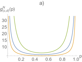
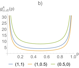
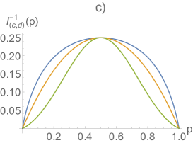
Figure 1: Fisher metric for $p=(p,1-p)$ corresponding to various $(c,d)$-deformations ($(c,d)=(1,1)$, $(1,1/2)$, $(1/2,0)$) for (a) Naudts type, (b) Amari type, and (c) the Cramér-Rao bound corresponding to the metric.

The metric of Amari type for the $(c,d)$-entropy was already discussed in ghikas17 based on $(c,d)$-logarithms. However, as demonstrated above, the metric can be found without using the inverse $\phi$-deformed logarithms, which in the case of $(c,d)$-logarithms lead to Lambert $W$-functions. The Fisher metric of Naudts and Amari type and the corresponding Cramér Rao bound is shown in Fig. 1. The scaling parameter is set (following ht11a ) to, $r=1/(1-c+cd)$, for $d\leq 0$, and $r=\exp(-d)/(1-c)$, for $d<0$. The Fisher metric of both types is displayed in Fig. 2 as a function of the parameters $c$ and $d$ for a given point, $P=(1/3,2/3)$. We see that both types of metric have a singularity for $(c,d)=(1,0)$. This point corresponds to distributions with compact support. For one-dimensional distributions the singularity corresponds to the transition between distributions with support on the real line and distributions with support on a finite interval.

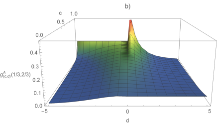
Figure 2: Fisher metric for $(c,d)$-deformations as a function of $c$ and $d$ of Naudts type (a), and Amari type (b). The metric is evaluated at a point $p=(1/3,2/3)$.

Interestingly, for $(c,d)=(q,0)$, the metric simplifies to

$$g_{(q,0),ij}^{A}(\bm{p})=\frac{2-q}{p_{i}}\delta_{ij}+\frac{2-q}{p_{0}}\quad,$$ (52)

which corresponds to Tsallis $q$-exponential family. Therefore, $g_{(q,0),ij}^{A}(p)$ is just a conformal transformation of the Fisher information metric for the exponential family, as shown in amari12 . Note, that only for Tsallis $q$-exponentials the relation between $S_{q}^{N}(p)$ and $S_{q}^{A}(p)$ can be expressed as (see also Table 2)

$$S_{q}^{A}(\bm{p})=f(S_{q^{\prime}}^{N}(\bm{p}))\quad,$$ (53)

where $f(x)=(2-q)/x$ and $q^{\prime}=2-q$. This is nothing but the well-known additive duality $q\leftrightarrow 2-q$ of Tsallis entropy tsallis05 . Interestingly, $q$-escort distributions form a group with $\phi_{q}(\phi_{q^{\prime}}(x))=(\phi_{q\cdot q^{\prime}}(x))$ and $\phi^{-1}_{q}(x)=\phi_{1/q}(x)$, where $q\leftrightarrow 1/q$ is the multiplicative duality tsallis17 . This is not the case for more general deformations, because typically, the inverse does not belong to the class of escort distributions. Popular deformations belonging to the $(c,d)$-family, as Tsallis $q$-exponential family or the stretched exponential family are summarized in Table 2.

V Connection to the deformed-log duality

A different duality of entropies and their associated logarithms under linear and escort averages has been discussed in htg12 . There, two approaches were discussed. The first is an approach using generalized entropy of trace form under linear constrains. It was denoted by

$$S^{HT}(\bm{p})=\sum_{i}s^{HT}(p_{i})=\sum_{i}\int_{0}^{p_{i}}\log^{HT}(x)\mathrm{d}x\quad.$$ (54)

It corresponds to the Naudts case here, $\log^{HT}(x)=\log_{\phi}^{N}(x)$. The second approach, originally introduced by Tsallis and Souza tsallis03 , uses the trace form entropy

$$S^{TS}(\bm{p})=\sum_{i}s^{TS}(p_{i})=\sum_{i}\int_{0}^{p_{i}}\log^{TS}(x)\mathrm{d}x\quad,$$ (55)

which is maximized under the escort constraints

$$\langle E\rangle_{TS}=\frac{\sum_{j}u(p_{j})E_{j}}{\sum_{j}u(p_{j})}\quad,$$ (56)

where $u(p_{j})=p_{j}+\nu s_{TS}(p_{j})$. The linear case is recovered for $\nu=0$. This form is dictated by the Shannon-Khinchin axioms, as discussed in the next section. Let us assume that the maximization of both approaches, Eq. (54) under linear, and Eq. (55) under escort constraints leads to the same MaxEnt distribution. One can then show that there exists the following duality (deformed-log duality) between $\log^{HT}(x)$ and $\log^{TS}$(x)

$$\log^{TS}(x)=\frac{1}{\frac{1}{\log^{HT}(x)}+\nu}$$ (57)

Let us focus on specific $\phi$-deformations, so that $\log^{HT}(x)=\log^{HT}_{\phi}(x)\equiv\log^{N}_{\phi}(x)$. Then, $\log^{TS}(x)$ is also a $\phi$-deformation, with

$$\phi^{TS}(x) = \phi^{HT}(x)\left(1+\nu\log_{\phi}^{HT}(x)\right)^{2}$$ (58)

$$= \phi^{HT}(x)\left(1+\nu\int_{1}^{x}\frac{1}{\phi^{HT}(y)}\mathrm{d}y\right)^{2}$$

It is straightforward to calculate the metric corresponding to the entropy $S^{TS}(\bm{p})$

$$g_{\phi,ij}^{TS}(\bm{p})=\frac{1}{\phi^{TS}(p_{i})}\delta_{ij}+\frac{1}{\phi^{TS}(p_{0})}\\ =\mathcal{T}_{\nu}(g_{\phi,ij}^{HT}(\bm{p}))\quad,$$

where

$$\mathcal{T}_{\nu}(g(x))=g(x)\left(1+\nu\int_{1}^{x}g(y)\mathrm{d}y\right)^{2}\quad.$$ (59)

Thus, the Tsallis-Souza approach results yet in another information matrix. We may also start from the other direction and look at the situation, when the escort distribution for the information geometric approach is the same as the escort distribution for the Tsallis-Souza approach. In this case we get that

$$\phi(x)=x+\nu s^{TS}(x)=x+\int_{0}^{x}\mathcal{T}_{\nu}(\log_{\phi}(y))\mathrm{d}y\quad.$$ (60)

We find that the entropy must be expressed as

$$S_{\phi}(\bm{p})=\sum_{i}\frac{\phi(p_{i})-p_{i}}{\nu}$$ (61)

Note that for $\phi(x)=x^{q}$, and $\nu=1-q$, we obtain Tsallis entropy

$$S_{\phi}(\bm{p})=\sum_{i}\frac{p_{i}^{q}-p_{i}}{1-q}\quad,$$ (62)

which corresponds to $S^{TS}(\bm{p})$ for $q^{\prime}=2-q$, which is nothing but the mentioned Tsallis additive duality. It turns out that Tsallis entropy is the only case where the deformed-log duality and the information geometric duality result in the same class of functionals. In general, the two dualities have different escort distributions.

	Tsallis $q$-exponential	Stretched $\eta$-exponential
$\phi(x)$	$x^{q}$	$x\eta\log(x)^{1-1/\eta}$
$\log_{\phi}(x)$	$\frac{x^{1-q}-1}{1-q}$	$\log(x)^{1/\eta}$
$\exp_{\phi}(x)$	$\left(1+(1-q)x\right)^{1/(1-q)}$	$\exp(x^{\eta})$
$\chi_{\phi}(x)$	$\frac{x}{q}$	$\frac{x\eta\log(x)}{(\eta-1)+\eta\log(x)}$
$S_{\phi}^{N}(\bm{p})$	$\frac{1}{q-1}\left(\sum_{i}\frac{p_{i}^{2-q}}{2-q}-1\right)$	$\sum_{i}\Gamma\left(\frac{\eta+1}{\eta},-\log p_{i}\right)$
$S_{\phi}^{A}(\bm{p})$	$\frac{1}{1-q}\left(\frac{1}{\sum_{i}p_{i}^{q}}-1\right)$	$\frac{\sum_{i}p_{i}\log p_{i}}{\sum_{i}p_{i}(\log p_{i})^{1-1/\eta}}$

Table 2: Two important special cases of $(c,d)$-deformations and related quantities: Power laws (Tsallis tsallis88 ) and stretched exponentials anteneodo99 .

VI Discussion

In this paper discuss the information geometric duality of entropies that are maximized by $\phi$-exponential distributions under two types of constraint: linear constraints that are known from contexts such as thermodynamics, and escort constraints, that appear naturally in the theory of statistical estimation and information geometry. This duality implies two different entropy functionals: $S^{N}(\bm{p})=-\sum_{i}\int_{0}^{p_{i}}\mathrm{d}x\log_{\phi}(x)$, and $S^{A}(\bm{p})=-\langle\log_{\phi}(P)\rangle_{\phi}$. For $\phi(x)=x$, they both boil down to Shannon entropy. The connection between the entropy of Naudts type and the one of Amari type can be established through the corresponding Fisher information through the Cramér-Rao bound. Contrary to the deformed-log duality introduced in htg12 , the information theoretic duality introduced here cannot be established within the framework of $\phi$-deformations, since $S^{A}(\bm{p})$ is not a trace form entropy. We demonstrated the duality between the Naudts approach with linear constraints, and the Amari approach with escort constraints, with the example of $(c,d)$-entropies, which include a wide class of popular deformations, including Tsallis and Anteneodo-Plastino entropy as special cases. Finally, we compared in detail the information geometric duality to the deformed-log duality, and showed that they are fundamentally different, and result in other types of Fisher information.

Let us now discuss the role of information geometric duality and possible applications in information theory and thermodynamics. Recall that the Shannon entropic functional is determined by the four Shannon-Khinchin (SK) axioms. In many different contexts at least three of the axioms should hold

• (SK1) Entropy is a continuous function of the probabilities $p_{i}$ only, and should not explicitly depend on any other parameters.

• (SK2) Entropy is maximal for the equi-distribution ${p}_{i}=1/W$.

• (SK3) Adding a state $W+1$ to a system with ${p}_{W+1}=0$ does not change the entropy of the system.

The fourth axiom that describes the composition rule for entropy (originally for Shannon entropy, $S(A+B)=S(A)+S(B|A)$). The only entropy satisfying all four SK axioms is Shannon entropy. However, Shannon entropy is not sufficient to describe statistics of complex systems ht11b , and can lead to paradoxes in applications in thermodynamics jensen18 . Therefore, instead of imposing the fourth axiom in situations where it does not apply, it is convenient to consider a weaker requirement, such as generic scaling relations of entropy in the thermodynamic limit ht11a ; korbel18 . It is possible to show that the only type of duality satisfying the first three Shannon-Khinchin axioms is the deformed-log duality of htg12 . Moreover, entropies which are neither trace-class, nor sum-class (i.e., in the form $f(\sum_{i}g(p_{i})$) might be problematic from the view of information theory and coding. For example, it is then not possible to consistently introduce a conditional entropy ilic13 because the corresponding conditional entropy cannot be properly defined. This is related to the fact that the Kolmogorov definition of conditional probability is not generally valid for escort distributions jizba17 . Additonal issues arise from the theory of statistical estimation, since only sum-class entropies can fulfil the consistency axioms uffink95 . From this point of view, the deformed-log duality using the class of Tsallis-Souza escort distributions can play the role in thermodynamical applications htg11 , because the corresponding entropy fulfils the SK axioms. On the other hand, the importance of escort distributions considered by Amari and others is in realm of information geometry (e.g., dually flat geometry or generalized Cramér-Rao bound), and their applications in thermodynamics might be limited. Finally, for the case of Tsallis $q$-deformation both dualities, the information geometric and the deformed-log duality reduce to the well-known additive duality $q\leftrightarrow 2-q$.

This work was supported by the Austrian Science Fund FWF under I 3073. All authors contributed to the conceptualization of the work, the discussion of the results, and their interpretation. JK took the lead in technical computations. JK and ST wrote the manuscript.

References

- [1] S. Thurner, B. Corominas-Murtra, and R. Hanel, Three faces of entropy for complex systems: Information, thermodynamics, and the maximum entropy principle. Physical Review E 96, 2017, 032124.
- [2] E. T. Jaynes, Information Theory and Statistical Mechanics. Phys. Rev. 106, 1957, 620.
- [3] P. Harremoës, and F. Topsøe, Maximum Entropy Fundamentals. Entropy 3, 2001, 191-226.
- [4] C. Tsallis, Possible generalization of Boltzmann-Gibbs statistics. Journal of statistical physics 52 (1-2), 1988, 479-487.
- [5] G. Kaniadakis, Statistical mechanics in the context of special relativity. Physical Review E 66, 2002, 056125.
- [6] P. Jizba and T. Arimitsu, The world according to Rényi: thermodynamics of multifractal systems. Annals of Physics 312(1), 2004, 17-59.
- [7] C. Tsallis and L. J. Cirto, Black hole thermodynamical entropy. The European Physical Journal C 73(7), 2013, 2487.
- [8] S. Thurner, R. Hanel and P. Klimek, Introduction to the theory of complex systems. Oxford University Press, 2018.
- [9] R. Hanel and S. Thurner, A comprehensive classification of complex statistical systems and an axiomatic derivation of their entropy and distribution functions. Europhysics Letters 93, 2011, 20006.
- [10] R. Hanel and S. Thurner, When do generalized entropies apply? How phase space volume determines entropy. Europhysics Letters 96, 2011, 50003.
- [11] C. Tsallis, M. Gell-Mann, and Y. Sato, Asymptotically scale-invariant occupancy of phase space makes the entropy extensive. PNAS 102 (43), 2005, 15377-15382.
- [12] H. J. Jensen, R. H. Pazuki, G. Pruessner and P. Tempesta, Statistical mechanics of exploding phase spaces: ontic open systems. Journal of Physics A 51, 2018, 375002.
- [13] J. Korbel, R. Hanel and S. Thurner, Classification of complex systems by their sample-space scaling exponents. New Journal of Physics 20, 2018, 093007.
- [14] C. Beck and E. D. G. Cohen, Superstatistics. Physica A 322, 2003, 267–275.
- [15] C. Tsallis, R. S. Mendes and A. R. Plastino, The role of constraints within generalized nonextensive statistics. Physica A 261(3-4), 1998, 534-554.
- [16] S. Abe, Geometry of escort distributions. Physical Review E 68, 2003, 031101.
- [17] A. Ohara, H. Matsuzoe and S. I. Amari, A dually flat structure on the space of escort distributions. Journal of Physics: Conference Series 201, 2010, 012012.
- [18] J.-F. Bercher, A simple probabilistic construction yielding generalized entropies and divergences, escort distributions and q-Gaussians. Physica A 391(19), 2012, 4460-4469.
- [19] R. Hanel, S. Thurner, and C. Tsallis, On the robustness of q-expectation values and Renyi entropy. Europhysics Letters 85, 2009, 20005.
- [20] R. Hanel, S. Thurner, and C. Tsallis, Limit distributions of scale-invariant probabilistic models of correlated random variables with the q-Gaussian as an explicit example. European Physical Journal B 72, 2009, 263-268.
- [21] C. Tsallis and A. M. C. Souza, Constructing a statistical mechanics for Beck-Cohen superstatistics. Physical Review E 67, 2003, 026106.
- [22] R. Hanel, S. Thurner, M. Gell-mann, Generalized entropies and logarithms and their duality relations. PNAS 109(47), 2012, 19151-19154.
- [23] S. I. Amari and A. Cichocki, Information geometry of divergence functions. Bulletin of the Polish Academy of Sciences: Technical Sciences, 58(1), 2010, 183-195.
- [24] S. I. Amari, A. Ohara and H. Matsuzoe, Geometry of deformed exponential families: Invariant, dually-flat and conformal geometries. Physica A 391(18), 2012, 4308-4319.
- [25] N. Ay, J. Jost, H. Vân Lê and L. Schwachhöfer, Information geometry. Springer Berlin, 2017.
- [26] J. Naudts, Deformed exponentials and logarithms in generalized thermostatistics. Physica A 316(1-4), 2002, 323-334.
- [27] J. Naudts, Continuity of a class of entropies and relative entropies. Reviews in Mathematical Physics 16(06), 2004, 809-822.
- [28] J. Naudts, Generalised thermostatistics, Springer Science & Business Media, 2011.
- [29] I. Csiszar, Why Least Squares and Maximum Entropy? An Axiomatic Approach to Inference for Linear Inverse Problems. Annuals of Statististics 19,1991, 2032-2066.
- [30] R. F. Vigelis and C. C. Cavalcante, On -Families of Probability Distributions, Journal of Theoretical Probability 26(3), 2013, 870-884.
- [31] A. Ohara, Conformal Flattening for Deformed Information Geometries on the Probability Simplex. Entropy 20(3), 2018, 186.
- [32] C. Anteneodo, A. R. Plastino, Maximum entropy approach to stretched exponential probability distributions, Journal of Physics A 32, 1999, 1089.
- [33] D. P. K. Ghikas and F. D. Oikonomou, Towards an information geometric characterization/classification of complex systems. I. Use of generalized entropies. Physica A 496, 2018, 384-398.
- [34] C. Tsallis, Generalization of the possible algebraic basis of -triplets. European Physics Journal Special Topics 226(3), 2017, 455-466.
- [35] R. Hanel, S. Thurner, M. Gell-mann, Generalized entropies and the transformation group of superstatistics. PNAS 108(16), 2011, 6390-6394.
- [36] V. M. Ilić and M. S. Stanković, Generalized Shannon–Khinchin axioms and uniqueness theorem for pseudo-additive entropies. Physica A 411, 2014, 138-145.
- [37] P. Jizba and J. Korbel, On the Uniqueness Theorem for Pseudo-Additive Entropies. Entropy 19(11), 2017, 605.
- [38] J. Uffink, Can the maximum entropy principle be explained as a consistency requirement? Studies in History and Philosophy of Science B, 26(3), 1995, 223-261.