A coarse-grained polymer model for studying the glass transition
Abstract
To study the cooling behavior and the glass transition of polymer melts in bulk and with free surfaces a coarse-grained weakly semi-flexible polymer model is developed. Based on a standard bead spring model with purely repulsive interactions an attractive potential between non-bonded monomers is added, such that the pressure of polymer melts is tuned to zero. Additionally, the commonly used bond bending potential controlling the chain stiffness is replaced by a new bond bending potential. For this model, we show that the Kuhn length and the internal distances along the chains in the melt only very weakly depend on temperature, just as for typical experimental systems. The glass transition is observed by the temperature dependency of the melt density and the characteristic non-Arrhenius slowing down of the chain mobility. The new model is set to allow for a fast switch between models, for which a wealth of data already exists.
pacs:
Polymer materials are omnipresent in our daily life with applications in medicine, technology as well as as ‘simple’ commodities to name a few. Very often these materials are in the glassy state Anantrao et al. (2017). In the liquid more rubbery state the viscosity dramatically increases close to the glass transition temperature in a non-Arrhenius way Boyd et al. (1994); Angell (1995); Paluch et al. (2001); Berthier and Biroli (2011). This slowing down of the chain mobility is of both high scientific and technological interest. Experimentally, of polymers can be determined as such by observing the change in the heat capacity of polymers using differential scanning calorimetry (DSC) Mathot (1994), or by measuring the thermal expansion coefficient using thermo mechanical analysis (TMA) Bird et al. (1987). However, the nature of the glass transition is still not fully understood Angell (1988, 1991); Binder and Kob (2005); Barrat et al. (2010); Stillinger and Debenedetti (2013); Ediger and Forrest (2014). It is the purpose of this communication to present a most simple, efficient bead spring model, which allows to study these effects and which can make contact to the huge body of simulation data available in the literature.
Computer simulations play an important role in investigating the structure and molecular motion (viscosity) of polymeric systems under a variety of different conditions. For studying glassy polymers, both atomistic and coarse-grained models are widely used in the literature Binder and Kob (2005); Barrat et al. (2010). The structure and thermal behavior of fluid mixtures can also be analyzed by tuning relative resolution in a recently developed hybrid model combing the fine-grained and coarse-grained models Chaimovich et al. (2015). Our aim is to eventually study generic properties of large and highly entangled polymer melts in bulk, in confinement and with free surfaces as a function of temperature within accessible computing times. For this we adopt a highly efficient coarse-grained model Kremer and Grest (1990). Usually in these models the excluded volume interaction is taken care of by a purely repulsive Lennard-Jones (LJ) potential, the Weeks-Chandler-Andersen (WCA) potential Kremer and Grest (1990), which prevents the study of surfaces Dünweg et al. (1997); Kopf et al. (1997) and displays a rather high pressure (, , density in standard Lennard-Jones (LJ) units of energy and length, and being the Boltzmann factor). To reduce the pressure the cut-off of the WCA potential for non-bonded pairs of monomers is often doubled from to , resulting Bennemann et al. (1998); Binder (1999); Buchholz et al. (2002); Binder et al. (2003); Schnell et al. (2011); Frey et al. (2015). The two main shortages of this setting are: (1) There is a small discontinuity in the force at the cut-off making microcanonical runs impossible and (2) the pressure is still not very close to zero. Furthermore, chain stiffness usually is taken into account by a bond bending potential Everaers et al. (2004); Svaneborg and Everaers (2018); Svaneborg et al. (2018), which tends to stretch the chains out with decreasing temperatures Grest (2016). As will be shown below, this leads to rather artificial chain conformations upon cooling, while in experiment chain conformations only very weakly depend on temperature Wind et al. (2003); Fetters et al. (2007). Our new coarse-grained model is set to overcome these shortages.
Our starting point is the standard bead spring model (BSM) Kremer and Grest (1990) with a weak bending elasticity Everaers et al. (2004) (the bending strength ) for which a huge body of data already exists (see e.g. Zhang et al. (2014); Moreira et al. (2015); Hsu and Kremer (2016, 2018a, 2018b); Svaneborg and Everaers (2018)). While focusing on , our approach easily applies to other bending constants as well. At the standard melt density of ( being the unit of length) the weak bending elasticity combined with the chain packing result in an entanglement length of only monomers. is small enough to allow for extremely efficient simulations of highly entangled, huge polymeric systems, while at the same time the subchain of length is already well described by a Gaussian chain. The purpose of this communication is to replace/extend the WCA excluded volume interaction potential to arrive at a pressure of , which allows to study free surfaces in interaction with gases, liquids, and particles for example, and to replace the standard bending potential by a new modified , which should lead to the typical very weak temperature dependence of chain conformations in melts. The close resemblance to the standard semiflexible bead spring model will allow to switch “on the fly” between the models and to make use of the already broadly available data.
(a)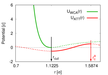 (b)
(b)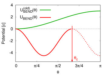
In a first step we add an attractive well to the WCA excluded volume in order to reduce the pressure in the system from to . For this we add (see Figure 1a),
| (4) |
between all non-bonded monomers. is set to not alter the local bead packing. It is chosen to have zero force at the cut-off as well as at the contact point between the two parts of the potential at , which is needed in the case microcanonical simulations are performed. As illustrated in Figure 2a, adding this term to the standard model equilibrates and reduces the pressure to zero in less than ( being the standard LJ unit of time). This time corresponds to a small, local bead displacement of about , for which the characteristic time is Hsu and Kremer (2016) . Furthermore, since the number of particles in the interaction range is instead of at or at using the standard LJ potential, the present model is computationally significantly more efficient. In the next step we replace the standard bond bending potential which would lead to a rod-like chain in the ground state at by a new bending potential with the goal to (1) match the chain conformations at and (2) to approximately preserve them upon cooling. Thus it should satisfy the condition that the mean square end-to-end distance of chains, , does not (preferably) or only very weakly depend on the temperature . The new bond bending potential (see Figure 1b) is chosen as
| (5) |
with the bond angle defined by where is the bond vector between monomers and along the chain. The fitting parameters and , and the cut-off where the force are adjusted such that the estimates of the mean square internal distance for all chemical distance between two monomers along the same chain follow the same curve as obtained from the model using with . Comparing to the reference data for a polymer melt of , shown in Figure 2b, we find that , . leads to an almost perfect match of the two systems. Our data are also in perfect agreement with the theoretical prediction described by a freely rotating chain (FRC) model Rubinstein and Colby (2003); Hsu and Kremer (2016).
(a)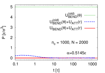 (b)
(b)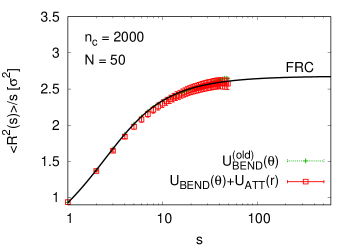
(c)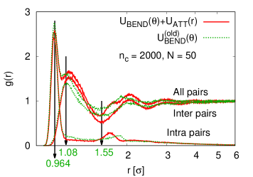 (d)
(d)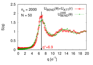
Compared to the original model, the profiles of the pair distribution function of all, inter, and intra pairs of monomers for polymer melts show that the two potentials and only have very small effects on the local packing of monomers (Figure 2c). Results of the collective structure factor also show that using the new model, the occurrence of the first peak remains at indicating the same mean distance between monomers in the first neighbor shell of the polymer melt. The peak itself is slightly higher, indicating a slightly more structured local environment, in agreement with the observed weakly enhanced bead friction.
(a)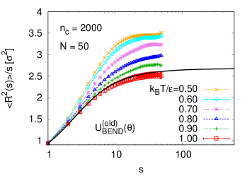 (b)
(b)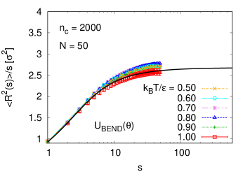
(c)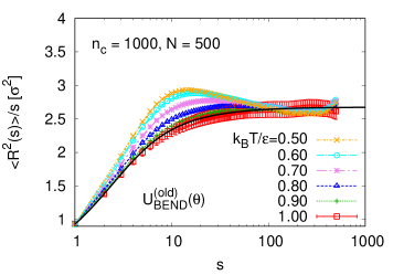 (d)
(d)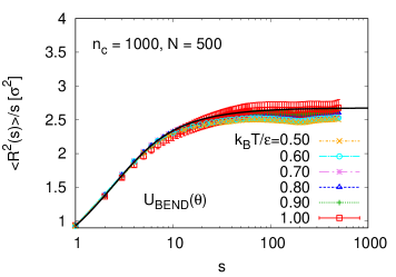
We now turn to the temperature dependency and compare melts of the new model to the standard semiflexible polymer model. For that we perform molecular dynamics (MD) simulations (Hoover Barostat with Langevin thermostat Martyna et al. (1994); Quigley and Probert (2004) implemented in ESPResSo++ Halverson et al. (2013)) at constant temperature by a stepwise cooling Buchholz et al. (2002), and constant pressure ( for the old model), i.e. in the isothermal-isobaric ensemble (NPT), for two polymer melts of , , and , , respectively. The temperature is reduced in steps of with a relaxation time between each step of resulting in a cooling rate of . corresponds to ( being the Rouse time of the chains at for the old model). Results of the mean square internal distances and the bond angle probability distribution, , are shown in Figures 3, 4. First let us focus on the standard weakly semiflexible model. As temperature decreases the chains stretch out as displayed in Figure 3a for . While for the cooling rate is slow enough to allow for equilibration over a wide temperature range, for longer chains (, Figure 3c) the system cannot equilibrate anymore even on short length scales (), leading to a characteristic maximum in . For long chain simulations, it will not be possible to avoid this artefact. Also the strong increase of of the standard semiflexible polymer model, is an artefact of the model when compared to experiments. This increase in chain stiffness is related to the shift of the probability distribution towards smaller angles as revealed in Figure 4a and which directly connects to the shape of the standard bending potential Schnell et al. (2011). In contrast, the new excluded volume and bending potential not only leads to a conformational very close match with the old one at , but it also avoids a significant temperature shift. Figure 4b demonstrates for that becomes independent of within the error bars. As a consequence we also do not observe the maximum in for as a function of temperature (Figure 3d). These observations fit to the dependence of the distribution , Figure 4b, which only becomes somewhat sharper but does not reveal any shift of the maximum.
(a)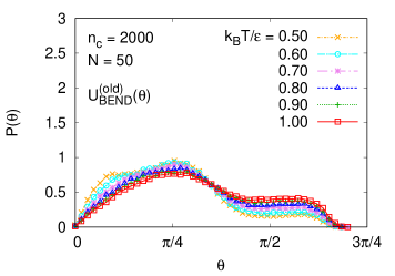 (b)
(b)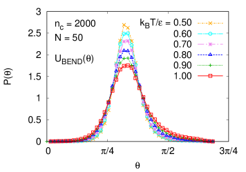
(a)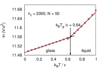 (b)
(b)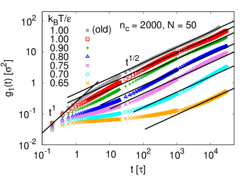
(c)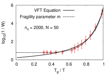
Finally we report some preliminary results for our new model in the glass transition region. As we are not interested here in details of the transition itself, we focus on () and one cooling rate (, which, however, allows for a full relaxation of the system up to the region very close to , the observed glass transition temperature. can be determined from the change of density or volume as a function of temperature Buchholz et al. (2002). The intersection of linear extrapolation of between the liquid branch () and glass branch () gives a good estimate of . Here and are thermal expansion coefficients for polymer melts in the liquid state and the glass state, respectively. Results of plotted versus are shown in Figure 5a. The glass transition occurs around . To investigate the mobility of chains at , we perform additional NVT MD simulations with a weak coupling Langevin thermostat for polymer melts at , , , , , , , and . The initial configuration and volume of the polymer melt at each temperature are taken from the last configuration of the NPT run in the cooling process. According to the Rouse model Rouse (1953), the mean square displacement (MSD) of monomers, , is expressed in terms of the Rouse rate as . Here being the monomeric friction coefficient is related to the self-diffusion coefficient and the viscosity using the Stokes-Einstein relation. Results of taking from the average MSD of inner monomers are shown in Figure 5b. We also include the data at for the old model for comparison. The Rouse rate depending on the temperature is determined by the best fit of a straight line with slope going through our data on log-log scales. At , the Rouse rate for the old model () is faster than the new model (). From the well-known Vogel-Fulcher-Tammann (VFT) equation Vogel (1921); Fulcher (1925); Tammann et al. (1926), , where , , and are constants and is the absolute temperature, Angell Angell (1988, 1991) has proposed that the fragility parameter , defined by Nascimento and Aparicio (2007): . Thus, plotting versus in Figure 5c, we obtain the characteristic behavior of a polymer approaching the glass transition.
In summary, based on the standard BSM, we have introduced a new non-bonded short range attractive potential and bond bending potential for studying polymer melts subject to cooling. The functional form of these two new interaction potentials also is directly applicable to other standard BSM models with different stiffness Svaneborg and Everaers (2018) just by adjusting the coefficients. By keeping , which results in a density of for all longest () systems within the error bars, we get for , and , , , and for , , , and , respectively. The new coarse-grained model captures the major features of glass-forming polymers, and preserves the Kuhn length as well as internal distances and can also be used to study systems with free surfaces. By construction it can directly take advantage of available simulation data of standard BSM models at and can be applied to available large deformed polymer melts Hsu and Kremer (2018a, b) and for understanding the viscoelastic behavior of these polymeric systems.
Acknowledgement: We are grateful to B. Dünweg for a critical reading of the manuscript. This work has been supported by European Research Council under the European Union’s Seventh Framework Programme (FP7/2007-2013)/ERC Grant Agreement No. 340906-MOLPROCOMP. We also gratefully acknowledge the computing time granted by the John von Neumann Institute for Computing (NIC) and provided on the supercomputer JUROPA at Jülich Supercomputing Centre (JSC), and the Max Planck Computing and Data Facility (MPCDF).
References
- Anantrao et al. (2017) J. H. Anantrao, J. C. Motichand, and B. S. Narhari, Int. J. Adv. Res. 5, 671 (2017).
- Boyd et al. (1994) R. H. Boyd, R. H. Gee, J. Han, and Y. Jin, J. Chem. Phys. 101, 788 (1994).
- Angell (1995) C. A. Angell, Science 267, 1924 (1995).
- Paluch et al. (2001) M. Paluch, J. Gapinski, A. Patkowski, and E. W. Fischer, J. Chem. Phys. 114, 8048 (2001).
- Berthier and Biroli (2011) L. Berthier and G. Biroli, Rev. Mod. Phys. 83, 587 (2011).
- Mathot (1994) V. B. F. Mathot, Calorimetry and thermal analysis of polymers (Hanser, Munich, 1994).
- Bird et al. (1987) R. Bird, C. Curtis, and R. Armstrong, Dynamics of Polymer Fluids, 2nd ed. (Wiley, New York, 1987).
- Angell (1988) C. A. Angell, J. Phys. Chem. Solids 49, 863 (1988).
- Angell (1991) C. A. Angell, J. Non-Cryst. Solids 131-133, Part 1, 13 (1991).
- Binder and Kob (2005) K. Binder and W. Kob, Glassy Materials and Disordered Solids (World Scientific, Singapore, 2005).
- Barrat et al. (2010) J.-L. Barrat, J. Baschnagel, and A. Lyulin, Soft Matter 6, 3430 (2010).
- Stillinger and Debenedetti (2013) F. H. Stillinger and P. G. Debenedetti, Annu. Rev. Condens. Matter Phys. 4, 263 (2013).
- Ediger and Forrest (2014) M. D. Ediger and J. A. Forrest, Macromolecules 47, 471 (2014).
- Chaimovich et al. (2015) A. Chaimovich, C. Peter, and K. Kremer, J. Chem. Phys. 143, 243107 (2015).
- Kremer and Grest (1990) K. Kremer and G. S. Grest, J. Chem. Phys. 92, 5057 (1990).
- Dünweg et al. (1997) B. Dünweg, G. S. Grest, and K. Kremer, Conf. Proc. of the IMA Workshop (Minneapolis MN, May 1996) (Berlin:Springer, 1997).
- Kopf et al. (1997) A. Kopf, B. Dünweg, and W. Paul, J. Chem. Phys. 107, 6945 (1997).
- Bennemann et al. (1998) C. Bennemann, W. Paul, K. Binder, and B. Dünweg, Phys. Rev. E 57, 843 (1998).
- Binder (1999) K. Binder, Comp. Phys. Commun. 121-122, 168 (1999).
- Buchholz et al. (2002) J. Buchholz, W. Paul, F. Varnik, and K. Binder, J. Chem. Phys. 117, 7364 (2002).
- Binder et al. (2003) K. Binder, J. Baschnagel, and W. Paul, Prog. Polym. Sci. 28, 115 (2003).
- Schnell et al. (2011) B. Schnell, H. Meyer, C. Fond, J. P. Wittmer, and J. Baschnagel, Eur. Phys. J. E 34, 97 (2011).
- Frey et al. (2015) S. Frey, F. Weysser, H. Meyer, J. Farago, M. Fuchs, and J. Baschnagel, Eur. Phys. J. E. 38, 11 (2015).
- Everaers et al. (2004) R. Everaers, S. K. Sukumaran, G. S. Grest, C. Svaneborg, A. Sivasubramanian, and K. Kremer, Science 303, 823 (2004).
- Svaneborg and Everaers (2018) C. Svaneborg and R. Everaers, arXiv:1808.03503 (2018).
- Svaneborg et al. (2018) C. Svaneborg, H. A. Karimi-Varzaneh, N. Hojdis, F. Fleck, and R. Everaers, arXiv:1808.03509 (2018).
- Grest (2016) G. S. Grest, J. Chem. Phys. 145, 141101 (2016).
- Wind et al. (2003) M. Wind, R. Graf, A. Heuer, and H. W. Spiess, Phys. Rev. Lett. 91, 155702 (2003).
- Fetters et al. (2007) L. J. Fetters, D. J. Lohse, and R. H. Colby, in Physical Properties of Polymers Handbook, 2nd, edited by J. E. Mark (Springer, New York, 2007) Chap. 25, pp. 447–454.
- Zhang et al. (2014) G. Zhang, L. A. Moreira, T. Stuehn, K. C. Daoulas, and K. Kremer, ACS Macro Lett. 3, 198 (2014).
- Moreira et al. (2015) L. A. Moreira, G. Zhang, F. Müller, T. Stuehn, and K. Kremer, Macromol. Theor. Simul. 24, 419 (2015).
- Hsu and Kremer (2016) H.-P. Hsu and K. Kremer, J. Chem. Phys. 144, 154907 (2016).
- Hsu and Kremer (2018a) H.-P. Hsu and K. Kremer, ACS Macro Lett. 7, 107 (2018a).
- Hsu and Kremer (2018b) H.-P. Hsu and K. Kremer, Phys. Rev. Lett. 121, 167801 (2018b).
- Rubinstein and Colby (2003) M. Rubinstein and R. H. Colby, Polymer Physics (Oxford University Press, Oxford, 2003).
- Martyna et al. (1994) G. J. Martyna, D. J. Tobias, and M. L. Klein, J. Chem. Phys. 101, 4177 (1994).
- Quigley and Probert (2004) D. Quigley and M. I. J. Probert, J. Chem. Phys. 120, 11432 (2004).
- Halverson et al. (2013) J. D. Halverson, T. Brandes, O. Lenz, A. Arnold, S. Bevc, V. Starchenko, K. Kremer, T. Stuehn, and D. Reith, Comput. Phys. Commun. 184, 1129 (2013).
- Rouse (1953) P. R. Rouse, J. Chem. Phys. 21, 1272 (1953).
- Vogel (1921) H. Vogel, Phys. Z 22, 645 (1921).
- Fulcher (1925) G. S. Fulcher, J. Am. Ceram. Soc. 8, 339 (1925).
- Tammann et al. (1926) G. Tammann, W. Hesse, and Z. Anorg, Allgem. Chem. 156, 245 (1926).
- Nascimento and Aparicio (2007) M. L. F. Nascimento and C. Aparicio, J. Phys. Chem. Solids 68, 104 (2007).