Exact Solution to a Dynamic SIR Model

Abstract

We investigate an epidemic model based on Bailey’s continuous differential system. In the continuous time domain, we extend the classical model to time-dependent coefficients and present an alternative solution method to Gleissner’s approach. If the coefficients are constant, both solution methods yield the same result. After a brief introduction to time scales, we formulate the SIR (susceptible-infected-removed) model in the general time domain and derive its solution. In the discrete case, this provides the solution to a new discrete epidemic system, which exhibits the same behavior as the continuous model. The last part is dedicated to the analysis of the limiting behavior of susceptible, infected, and removed, which contains biological relevance.

MSC 2010: 92D25; 34N05.

Keywords: dynamic equations on time scales; deterministic epidemic model; closed-form solution; time-varying coefficients; asymptotic behavior.

1 Introduction

Modeling infectious diseases is as important as it has been in 1760, when Daniel Bernoulli presented a solution to his mathematical model on smallpox. It was however not until the $20$th century that mathematical models became a recognized tool to study the causes and effects of epidemics. In 1927, Kermack and McKendrick introduced their SIR-model based on the idea of grouping the population into susceptible, infected, and removed. The model assumes a constant total population and an interaction between the groups determined by the disease transmission and removal rates. Although the removed represent in some models the vaccinated individuals, it can also be used to transform a time dependent population size into a constant population. In the latter case, the total number of contacts that a susceptible individual could get in contact with, is not the individuals of all three groups but $x+y$, where $x$ is the number of susceptible and $y$ the number of infected individuals. Let $k$ be the actual number of individuals a susceptible interacts with and $p$ be the probability that a susceptible gets infected at contact with an infected individual. Then $pk\frac{y}{x+y}$ is the rate at which one susceptible enters the group of infected [1]. This leads to the rate of change for the group of susceptible as

$$\frac{{\rm d}x}{{\rm d}t}=-pk\frac{y}{x+y}x.$$

Similarly, the infected increase by that rate, but some infected leave the class of infected, due to death for example, at a rate $c$, which yields the differential equation in $y$ as

$$\frac{{\rm d}y}{{\rm d}t}=pk\frac{y}{x+y}x-cy.$$

To obtain a system with time independent sum, a third group is added, the group of removed individuals for example, denoted by $z$, with the dynamics given by

$$\frac{{\rm d}z}{{\rm d}t}=cy.$$

Many modifications of the classical model have been investigated such as models with vital dynamics, see [2, 3, 4]. To model the spreading of diseases between different states, a spatial variable was added, which led to a partial differential system, see [5, 6]. Already in 1975, Bailey discussed in [1] the relevance of stochastic terms in the mathematical model of epidemics, which is still an attractive way of modeling the uncertainty of the transmission and vaccines, see [7, 8, 9, 10]. Although these modifications exist, so far there has been no success in generalizing the epidemic models to a general time scale to allow modeling a noncontinuous disease dynamics. A disease, where the virus remains within the host for several years unnoticed before continuing to spread, is only one example that can be modeled by time scales. We trust that this work provides the foundation for further research on generalizing epidemic models to allow modeling of discontinuous epidemic behavior.

2 Continuous SIR Model

We investigate a susceptible-infected-removed (SIR) model proposed by Norman Bailey in [1] of the form

$$\begin{cases}x^{\prime}=-\frac{bxy}{x+y},&\\ y^{\prime}=\frac{bxy}{x+y}-cy,&\\ z^{\prime}=cy,&\end{cases}$$ (1)

with initial conditions $x(t_{0})=x_{0}>0$, $y(t_{0})=y_{0}>0$, $z(t_{0})=z_{0}\geq 0$, $x,y,z:\mathbb{R}\to\mathbb{R}_{0}^{+}$, and $b,c\in\mathbb{R}_{0}^{+}$. The variable $x$ represents the group of susceptible, $y$ the infected population, and $z$ the removed population. By adding the group of removed, the total population $N=x+y+z$ remains constant. In [11], assuming $x,y>0$, the model is solved by rewriting the first two equations in (1) as

$$\begin{cases}\frac{x^{\prime}}{x}=-\frac{b}{x+y}y,&\\ \frac{y^{\prime}}{y}=\frac{bx}{x+y}-c.&\\ \end{cases}$$

Subtracting these equations yields

$$\frac{x^{\prime}}{x}-\frac{y^{\prime}}{y}=-b+c,$$

i.e.,

$$\frac{y^{\prime}}{y}=\frac{x^{\prime}}{x}+b-c,$$

which is equivalent to

$$(\ln y)^{\prime}=(\ln x)^{\prime}+(b-c).$$

Integrating both sides and taking the exponential, one gets

$$y=x\kappa e^{(b-c)(t-t_{0})},\quad\mbox{ where }\kappa=\frac{y_{0}}{x_{0}}.$$ (2)

If $b\neq c$, then, plugging this into the first equation in (1) yields a first order linear homogeneous differential equation with the solution given by

$$x(t)=x_{0}\left(1+\kappa\right)^{\frac{b}{b-c}}\left(1+\kappa e^{(b-c)(t-t_{0})}\right)^{-\frac{b}{b-c}}.$$ (3)

Replugging yields the solution of (1) as

$$\begin{cases}x(t)=x_{0}(1+\kappa)^{\frac{b}{b-c}}(1+\kappa e^{(b-c)(t-t_{0})})^{-\frac{b}{b-c}},\\ y(t)=y_{0}(1+\kappa)^{\frac{b}{b-c}}(1+\kappa e^{(b-c)(t-t_{0})})^{-\frac{b}{b-c}}e^{(b-c)(t-t_{0})},\\ z(t)=N-(x_{0}+y_{0})^{\frac{b}{b-c}}(x_{0}+y_{0}e^{(b-c)(t-t_{0})})^{-\frac{c}{b-c}}.\end{cases}$$ (4)

If $b=c$, then (2) gives $y=x\kappa$, and the solution (4) of (1) is

$$\begin{cases}x(t)=x_{0}e^{-\frac{b\kappa(t-t_{0})}{1+\kappa}},&\\ y(t)=y_{0}e^{-\frac{b\kappa(t-t_{0})}{1+\kappa}},&\\ z(t)=N-(x_{0}+y_{0})e^{-\frac{b\kappa(t-t_{0})}{1+\kappa}}.&\\ \end{cases}$$

In this work, we present a different method to solve (1), considering not only constant $b,c$ but $b,c:\mathbb{R}\to\mathbb{R}^{+}$. This will allow us to find the solution to the model on time scales. To this end, define $w:=\frac{x}{y}>0$ for $x,y>0$ to get

$$w^{\prime}=\frac{x^{\prime}y-y^{\prime}x}{y^{2}}=\frac{\frac{-b(t)xy}{x+y}y-\left(\frac{b(t)xy}{x+y}-c(t)y\right)x}{y^{2}}=\frac{-b(t)xy+c(t)xy}{y^{2}}=(c-b)(t)w,$$

which is a first-order homogeneous differential equation with solution

$$w(t)=w_{0}e^{\int_{t_{0}}^{t}(c-b)(s)\,{\rm d}s},$$

i.e.,

$$y(t)=\kappa e^{\int_{t_{0}}^{t}(b-c)(s)\,{\rm d}s}x(t),$$ (5)

which is the same as (2) for constant $b,c$. We plug (5) into (1) to get

$$x^{\prime}=-\frac{b(t)x^{2}\kappa e^{\int_{t_{0}}^{t}(b-c)(s)\,{\rm d}s}}{x+\kappa xe^{\int_{t_{0}}^{t}(b-c)(s)\,{\rm d}s}}=-\frac{b(t)\kappa e^{\int_{t_{0}}^{t}(b-c)(s)\,{\rm d}s}}{1+\kappa e^{\int_{t_{0}}^{t}(b-c)(s)\,{\rm d}s}}x,$$

which has the solution

$$x(t)=x_{0}\exp\left\{-\kappa\int_{t_{0}}^{t}b(s)\left(\kappa+e^{\int_{t_{0}}^{s}(c-b)(\tau)\,{\rm d}\tau}\right)^{-1}\,{\rm d}s\right\}.$$ (6)

Note that, for constant $b,c$ with $b\neq c$, (6) simplifies to (3). Hence, the solution to (1) is given by

$$\begin{cases}x(t)=x_{0}\exp\left\{-\kappa\int_{t_{0}}^{t}b(s)\left(\kappa+e^{\int_{t_{0}}^{s}(c-b)(\tau)\,{\rm d}\tau}\right)^{-1}\,{\rm d}s\right\},&\\[5.69054pt] y(t)=y_{0}\exp\left\{\int_{t_{0}}^{t}\left[b(s)\left(1+\kappa e^{\int_{t_{0}}^{s}(b-c)(\tau)\,{\rm d}\tau}\right)^{-1}-c(s)\right]\,{\rm d}s\right\},&\\[5.69054pt] z(t)=N-\left(y_{0}e^{\int_{t_{0}}^{t}(b-c)(s)\,{\rm d}s}+x_{0}\right)\exp\left\{-\kappa\int_{t_{0}}^{t}b(s)\left(\kappa+e^{\int_{t_{0}}^{s}(c-b)(\tau)\,{\rm d}\tau}\right)^{-1}\,{\rm d}s\right\}.&\\ \end{cases}$$ (7)

The time-varying parameters $b$ and $c$ allow us to investigate epidemic models, where the transmission rate peaks in early years before reducing, for example due to initial ignorance but increasing precaution of susceptibles. This behavior could be described by the probability density function of the log-normal distribution. A removal rate that increases rapidly to a constant rate could be modeled by a “von Bertalanffy” type function, see Figure 1.

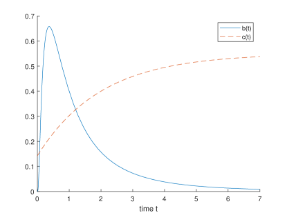
Figure 1: Time-varying parameters $b$ and $c$ of “von Bertalanffy” type: $b(t)=\frac{1}{t\sqrt{2\pi}}e^{-\frac{\ln^{2}(t)}{2}}$ and $c(t)=0.55\left(1-e^{-0.5t-0.3}\right)$.

Using these parameter functions with initial conditions $x_{0}=0.4$ and $y_{0}=1.2$ leads to the behavior in Figure 2. We see that the group of infected increases before reducing due to an increasing removal rate $c$. Zooming into the last part of the time interval, we see that the number of susceptibles converges.

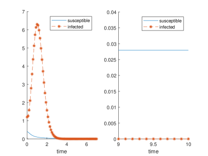
Figure 2: Dynamics of the susceptible $x$ and the infected $y$ populations with initial conditions $x_{0}=0.4$ and $y_{0}=1.2$ in the case of the time-varying coefficients $b$ and $c$ of Figure 1.

Example 1.

Considering a simple decreasing transmission rate to account for the rising precaution of susceptibles and a simple decreasing removal rate accounting for medical advances, for example by choosing $b(t)=\frac{1}{t+1}$ and $c(t)=\frac{2}{t+1}$, the solution with $t_{0}=0$ is given by (7) as

$$\begin{cases}x(t)=x_{0}\exp\left\{\int_{0}^{t}\frac{-\kappa}{(s+1)(\kappa+s+1)}\,{\rm d}s\right\}=x_{0}\frac{\kappa+1+t}{(\kappa+1)(t+1)},&\\[7.11317pt] y(t)=y_{0}\exp\left\{\frac{1}{\kappa+1+s}-\frac{2}{s+1}\right\}=y_{0}\frac{\kappa+1+t}{(\kappa+1)(t+1)^{2}},&\\[7.11317pt] z(t)=N-\frac{1+\kappa+t}{t+1}\left\{\frac{x_{0}}{\kappa+1}-\frac{y_{0}}{(\kappa+1)(t+1)}\right\},&\end{cases}$$

where $N=x_{0}+y_{0}+z_{0}$ and $\kappa=\frac{y_{0}}{x_{0}}$.

3 Time Scales Essentials

In order to formulate the time scales analogue to the model proposed by Norman Bailey, we first introduce fundamentals of time scales that we will use. The following introduces the main definitions in the theory of time scales.

Definition 2 (See [12, Definition 1.1]).

For $t\in\mathbb{T}$, the forward jump operator $\sigma:\mathbb{T}\to\mathbb{T}$ is

$$\sigma(t):=\inf\{s\in\mathbb{T}:s\,>t\}.$$

For any function $f:\mathbb{T}\to\mathbb{R}$, we put $f^{\sigma}=f\circ\sigma$. If $t\in\mathbb{T}$ has a left-scattered maximum $M$, then we define $\mathbb{T}^{\kappa}=\mathbb{T}\setminus\{M\}$; otherwise, $\mathbb{T}^{\kappa}=\mathbb{T}$.

Definition 3 (See [13, Definition 1.24]).

A function $p:\mathbb{T}\to\mathbb{R}$ is called rd-continuous provided $p$ is continuous at $t$ for all right-dense points $t$ and the left-sided limit exists for all left-dense points $t$. The set of rd-continuous functions is denoted by ${\rm C}_{\rm rd}={\rm C}_{\rm rd}(\mathbb{T})={\rm C}_{\rm rd}(\mathbb{T},\mathbb{R})$.

Definition 4 (See [12, Definition 2.25]).

A function $p:\mathbb{T}\to\mathbb{R}$ is called regressive provided

$$1+\mu(t)p(t)\neq 0\quad\mbox{ for all }t\in\mathbb{T},\quad\mbox{where }\mu(t)=\sigma(t)-t.$$

The set of regressive and rd-continuous functions is denoted by $\mathcal{R}=\mathcal{R}(\mathbb{T})=\mathcal{R}(\mathbb{T},\mathbb{R})$. Moreover, $p\in\mathcal{R}$ is called positively regressive, denoted by $\mathcal{R^{+}}$, if

$$1+\mu(t)p(t)>0\quad\mbox{ for all }t\in\mathbb{T}.$$

Definition 5 (See [12, Definition 1.10]).

Assume $f:\mathbb{T}\to\mathbb{R}$ and $t\in\mathbb{T}^{\kappa}$. Then the derivative of $f$ at $t$, denoted by $f^{\Delta}(t)$, is the number such that for all $\varepsilon>0$, there exists $\delta>0$, such that

$$\left|f(\sigma(t))-f(s)-f^{\Delta}(t)(\sigma(t)-s)\right|\leq\varepsilon\left|\sigma(t)-s\right|$$

for all $s\in(t-\delta,t+\delta)\cap\mathbb{T}$.

Theorem 6 (See [12, Theorem 2.33]).

Let $p\in\mathcal{R}$ and $t_{0}\in\mathbb{T}$. Then

$$y^{\Delta}=p(t)y,\quad y(t_{0})=1$$

possesses a unique solution, called the exponential function and denoted by $e_{p}(\cdot,t_{0})$.

Useful properties of the exponential function are the following.

Theorem 7 (See [12, Theorem 2.36]).

If $p\in\mathcal{R}$, then

1. $e_{0}(t,s)=1$, and $e_{p}(t,t)=1$,

2. $e_{p}(t,s)=\frac{1}{e_{p}(s,t)}$,

3. the semigroup property holds: $e_{p}(t,r)e_{p}(r,s)=e_{p}(t,s)$.

Theorem 8 (See [12, Theorem 2.44]).

If $p\in\mathcal{R}^{+}$ and $t_{0}\in\mathbb{T}$, then $e_{p}(t,t_{0})>0$ for all $t\in\mathbb{T}$.

We define a “circle-plus” and “circle-minus” operation.

Definition 9 (See [13, p. 13]).

Define the “circle plus” addition on $\mathcal{R}$ as

$$p\oplus q=p+q+\mu pq$$

and the “circle minus” subtraction as

$$p\ominus q=\frac{p-q}{1+\mu q}.$$

It is not hard to show the following identities.

Corollary 10 (See [12]).

If $p,q\in\mathcal{R}$, then

• $e_{p\oplus q}(t,s)=e_{p}(t,s)e_{q}(t,s),$

• $e_{\ominus p}(t,s)=e_{p}(s,t)=\frac{1}{e_{p}(t,s)}.$

Theorem 11 (Variation of Constants, see [12, Theorems 2.74 and 2.77]).

Suppose $p\in\mathcal{R}$ and $f\in{\rm C}_{\rm rd}$. Let $t_{0}\in\mathbb{T}$ and $y_{0}\in\mathbb{R}$. The unique solution of the IVP

$$y^{\Delta}=p(t)y+f(t),\quad y(t_{0})=y_{0}$$

is given by

$$y(t)=e_{p}(t,t_{0})y_{0}+\int_{t_{0}}^{t}e_{p}(t,\sigma(s))f(s)\,\Delta s.$$

The unique solution of the IVP

$$y^{\Delta}=-p(t)y^{\sigma}+f(t),\quad y(t_{0})=y_{0}$$

is given by

$$y(t)=e_{\ominus p}(t,t_{0})y_{0}+\int_{t_{0}}^{t}e_{\ominus p}(t,s)f(s)\,\Delta s.$$

Lemma 12 (See [12, Theorem 2.39]).

If $p\in\mathcal{R}$ and $a,b,c\in\mathbb{T}$, then

$$\int_{a}^{b}p(t)e_{p}(t,c)\Delta t=e_{p}(b,c)-e_{p}(a,c)$$

and

$$\int_{a}^{b}p(t)e_{p}(c,\sigma(t))\Delta t=e_{p}(c,a)-e_{p}(c,b).$$

4 Dynamic SIR Model

In this section, we formulate a dynamic epidemic model based on Bailey’s classical differential system (1) and derive its exact solution. In the special case of a discrete time domain, this provides a novel model as a discrete analogue of the continuous system. We end the discussion by analyzing the stability of the solutions to the dynamic model in the case of constant coefficients.

Consider the dynamic susceptible-infected-removed model of the form

$$\begin{cases}x^{\Delta}=-\frac{b(t)xy^{\sigma}}{x+y},&\\[5.69054pt] y^{\Delta}=\frac{b(t)xy^{\sigma}}{x+y}-c(t)y^{\sigma},&\\[5.69054pt] z^{\Delta}=c(t)y^{\sigma},&\\ x,y>0,&\\ \end{cases}$$ (8)

with given initial conditions $x(t_{0})=x_{0}>0$, $y(t_{0})=y_{0}>0$, $z(t_{0})=z_{0}\geq 0$, $x,y:\mathbb{T}\to\mathbb{R}^{+}$, $z:\mathbb{T}\to\mathbb{R}_{0}^{+}$, and $b,c:\mathbb{T}\to\mathbb{R}_{0}^{+}$.

Theorem 13.

If $c-b,g\in\mathcal{R}$, then the unique solution to the IVP (8) is given by

$$\begin{cases}x(t)=e_{\ominus g}(t,t_{0})x_{0},&\\ y(t)=e_{\ominus(g\oplus(c-b))}(t,t_{0})y_{0},&\\ z(t)=N-e_{\ominus g}(t,t_{0})\left(x_{0}+y_{0}e_{\ominus(c-b)}(t,t_{0})\right),\\ \end{cases}$$

where $N=x_{0}+y_{0}+z_{0}$, $\kappa=\frac{y_{0}}{x_{0}}$, and

$$g(t):=\frac{b(t)\kappa}{\kappa(1+\mu(t)(c-b)(t))+e_{c-b}(\sigma(t),t_{0})}.$$

Proof.

Assume that $x,y,z$ solve (8). Since $(x+y+z)^{\Delta}=0$, we get $z=N-(x+y)$, where $N=x_{0}+y_{0}+z_{0}$. Defining $w:=\frac{x}{y}$, we have

$$w^{\Delta}=\frac{x^{\Delta}y-y^{\Delta}x}{yy^{\sigma}}=\frac{\frac{-b(t)xy^{\sigma}}{x+y}y-\left(\frac{b(t)xy^{\sigma}}{x+y}-c(t)y^{\sigma}\right)x}{yy^{\sigma}}=\frac{-b(t)xy^{\sigma}+c(t)xy^{\sigma}}{yy^{\sigma}}=(c-b)(t)w,$$

which is a first-order linear dynamic equation with solution

$$w(t)=e_{c-b}(t,t_{0})w_{0},$$

i.e.,

$$y(t)=\kappa e_{\ominus(c-b)}(t,t_{0})x(t).$$ (9)

We plug (9) into (8) to get

$$x^{\Delta}=-\frac{b(t)xx^{\sigma}e_{\ominus(c-b)}(\sigma(t),t_{0})\kappa}{x+xe_{\ominus(c-b)}(t,t_{0})\kappa}=-\frac{b(t)e_{\ominus(c-b)}(\sigma(t),t_{0})\kappa}{1+e_{\ominus(c-b)}(t,t_{0})\kappa}x^{\sigma}=-g(t)x^{\sigma},$$

which has the solution

$$x(t)=e_{\ominus g}(t,t_{0})x_{0}.$$

By (9), we obtain

$$y(t)=y_{0}e_{\ominus(g\oplus(c-b))}(t,t_{0}),$$

and thus,

$$z(t)=N-x(t)-y(t)=N-e_{\ominus g}(t,t_{0})\left(x_{0}+y_{0}e_{\ominus(c-b)}(t,t_{0})\right).$$

This shows that $x,y,z$ are as given in the statement. Conversely, it is easy to show that $x,y,z$ as given in the statement solve (8). The proof is complete. ∎

Remark 14.

If $c-b\in\mathcal{R}^{+}$ and $x_{0}>0$, $y_{0},z_{0}\geq 0$, then $x,y,z\geq 0$ for all $t\in\mathbb{T}$. For $\mathbb{T}=\mathbb{R}$, this condition is satisfied, since $\mu(t)=0$ for all $t\in\mathbb{R}$.

Remark 15.

If $b(t)=c(t)$ for all $t\in\mathbb{T}$, then $c-b\in\mathcal{R}$, and, by Theorem 13, the solution of (8) is

$$\begin{cases}x(t)=e_{\ominus g}(t,t_{0})x_{0},&\\ y(t)=e_{\ominus g}(t,t_{0})y_{0},&\\ z(t)=N-e_{\ominus g}(t,t_{0})\left(x_{0}+y_{0}\right),&\end{cases}$$

where

$$g(t)=\frac{b(t)\kappa}{1+\kappa}.$$

As an application of Theorem 13, we introduce the discrete epidemic model

$$\begin{cases}x(t+1)=x(t)-\frac{b(t)x(t)y(t+1)}{x(t)+y(t)},&\\[5.69054pt] y(t+1)=y(t)+\frac{b(t)x(t)y(t+1)}{x(t)+y(t)}-c(t)y(t+1),&\\[5.69054pt] z(t+1)=z(t)+c(t)y(t+1),&\end{cases}$$ (10)

$t\in\mathbb{Z}$, with initial conditions $x(t_{0})=x_{0}>0$, $y(t_{0})=y_{0}>0$, $z(t_{0})=z_{0}\geq 0$. Note that the second equation of (10) can be represented as

$$y(t+1)=\frac{1}{1+\delta(t)}y(t),$$

which implies that a fraction, namely $\frac{1}{1+\delta}$, of the infected individuals remain infected. If the rate with which susceptibles are getting infected is higher than the rate with which infected are removed, i.e., $\varphi=b\frac{x}{x+y}>c$, then the multiplicative factor $\delta=c-\varphi$ is greater than one, else less than one. Slightly rewriting the first equation into the form

$$x(t+1)+\varphi(t)y(t+1)=x(t)$$

provides the interpretation that some susceptible individuals stay in the group of susceptibles, others become infected and contribute the fraction $\varphi$ to the group of infected. A similar inference can be drawn from

$$z(t+1)=z(t)+c(t)y(t+1).$$

The number of removed individuals is the sum of the already removed individuals and a proportion of infected individuals that are removed at the end of the time step.

The following theorem is a direct consequence of Theorem 13.

Theorem 16.

If $1+c(t)-b(t),1+g(t)\neq 0$ for all $t\in\mathbb{Z}$, where

$$g(t)=\frac{b(t)\kappa}{\left[\prod_{i=t_{0}}^{t}(1+(c-b)(i))\right]+\kappa(1+(c-b)(t))},$$

then the unique solution to (10) is given by

$$\begin{cases}x(t)=x_{0}\left[\prod_{i=t_{0}}^{t-1}\left(1+g(i)\right)\right]^{-1},&\\[5.69054pt] y(t)=y_{0}\left[\prod_{i=t_{0}}^{t-1}(1+(c-b)(i))(1+g(i))\right]^{-1},&\\[5.69054pt] z(t)=N-\left(x_{0}+y_{0}\left[\prod_{i=t_{0}}^{t-1}(1+(c-b)(i))\right]^{-1}\right)\left[\prod_{i=t_{0}}^{t-1}\left(1+g(i)\right)\right]^{-1},&\end{cases}$$

where $N=x_{0}+y_{0}+z_{0}$ and $\kappa=\frac{y_{0}}{x_{0}}$.

Example 17.

Consider a disease with periodic transmission rate, for example due to sensitivity of bacteria to temperature or hormonal cycles. In this case, we might choose $b(t)=\frac{1}{2}+\frac{1}{4}\sin(mt)$ with $m\in\mathbb{R}\backslash\{0\}$. To account for medical advances, we let $c(t)=\frac{1}{t+1}$. Note that $1+c(t)\neq b(t)$ because $\frac{1}{4}\leq b(t)\leq\frac{3}{4}<1$ and $1+g(t)\neq 0$ for all $t\in\mathbb{Z}$. The solution is then given by Theorem 16 with

$$g(t)=\frac{2+\sin(mt)}{\left[\frac{4}{\kappa}\prod_{i=t_{0}}^{t}\frac{3+i}{2(1+i)}-\frac{1}{4}\sin(mi)\right]+\frac{2(3+t)}{1+t}-\sin(mt)}.$$

Remark 18.

If $\mathbb{T}=\mathbb{R}$, $b,c\in\mathbb{R}$, $b\neq c$, and $t_{0}=0$, then, by Theorem 13, the solution to (8) is

$$x(t) =x_{0}e^{-\int_{0}^{t}g(s)\,{\rm d}s}=x_{0}e^{-b\int_{0}^{t}\frac{\kappa e^{-(c-b)s}}{1+\kappa e^{-(c-b)s}}\,{\rm d}s}=x_{0}e^{-\frac{b}{b-c}\left(\ln(1+\kappa e^{-(c-b)t})-\ln(1+\kappa)\right)}$$

$$=x_{0}\left(1+\kappa e^{-(c-b)t}\right)^{-\frac{b}{b-c}}\left(1+\kappa\right)^{\frac{b}{b-c}},$$

which is consistent with (3). If $c=b$, then Theorem 13 provides the solution as

$$x(t)=x_{0}e^{-\int_{0}^{t}g(s)\,ds}=x_{0}e^{-b\int_{0}^{t}\frac{\kappa}{1+\kappa}\,ds}=x_{0}e^{\frac{-b\kappa}{1+\kappa}t},$$

which is consistent with the continuous results.

Example 19.

Let us consider the SIR model (8) with

$$b=0.4,\quad c=0.2,\quad x_{0}=0.8,\quad y_{0}=0.2,\quad z_{0}=0.$$

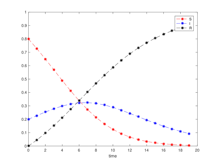
(a) $\mathbb{T}=\mathbb{Z}$

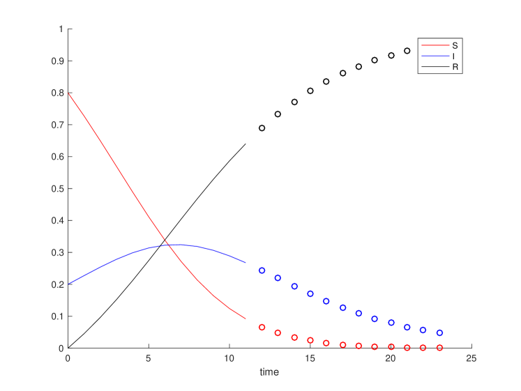
(b) $\mathbb{T}=[0,12]\cup\{13,14,15,\ldots,24\}$

Figure 3: the $x$=Susceptible ($S$), $y$=Infected ($I$), and $z$=Removed ($R$) dynamics of Example 19.

In Figure 3(a), we show the solution in the discrete-time case $\mathbb{T}=\mathbb{Z}$ determined by (10); in Figure 3(b), we plot the solution to (8) for the partial continuous, partial discrete time scale $\mathbb{T}=[0,12]\cup\{13,\ldots,24\}$.

5 Long Term Behavior

We start this section by recalling the following results.

Lemma 20 (See [14, Lemma 3.2]).

If $p\in\mathcal{R}^{+}$, then

$$0<e_{p}(t,t_{0})\leq\exp\left\{\int_{t_{0}}^{t}p(\tau)\Delta\tau\right\}\quad\quad\mbox{for all }t\geq t_{0}.$$

Lemma 21 (See [15, Remark 2]).

If $p\in{\rm C}_{\rm rd}$ and $p(t)\geq 0$ for all $t\in\mathbb{T}$, then

$$1+\int_{t_{0}}^{t}p(\tau)\Delta\tau\leq e_{p}(t,t_{0})\leq\exp\left\{\int_{t_{0}}^{t}p(\tau)\Delta\tau\right\}\quad\quad\mbox{for all }t\geq t_{0}.$$

The equilibriums of (8) are given as follows.

Lemma 22.

Suppose $c(t)>0$ for some $t\in\mathbb{T}$. The equilibriums of (8) are given by the plane $(\alpha,0,N-\alpha)$, where $\alpha\in[0,N]$ and $N=x_{0}+y_{0}+z_{0}$.

Proof.

Assume $x,y,z$ are constant solutions of (8). Then, $0=z^{\Delta}(t)=c(t)y(t)$, so $y(t)=0$ for all $t\in\mathbb{T}$. Therefore,

$$-\frac{b(t)xy}{x+y}=x^{\Delta}=0=y^{\Delta}=\frac{b(t)xy}{x+y}-c(t)y\quad\mbox{ for any }0\leq x\leq N$$

and the proof is complete. ∎

Theorem 23.

Consider (8) and assume $\mathbb{T}$ is unbounded from above. Assume $b,c:\mathbb{T}\to\mathbb{R}_{0}^{+}$, $c-b\in\mathcal{R}^{+}$, $x_{0},y_{0}>0$, and $z_{0}\geq 0$. Moreover, assume

$$\exists\,L>0:\,\int_{t_{0}}^{t}(c-b)(\tau)\,\Delta\tau\leq L\quad\quad\mbox{ for all }t\geq t_{0}$$ (11)

and

$$\int_{t_{0}}^{\infty}\frac{b(\tau)}{1+\mu(\tau)(c-b)(\tau)}\,\Delta\tau=\infty.$$ (12)

Then all solutions of (8) converge to the equilibrium $(0,0,N)$, where $N=x_{0}+y_{0}+z_{0}$.

Proof.

By Lemma 20,

$$0<e_{c-b}(t,t_{0})\leq e^{\int_{t_{0}}^{t}(c-b)(\tau)\,\Delta\tau}\stackrel{{\scriptstyle\eqref{ProofBEq1}}}{{\leq}}e^{L},\quad t\geq t_{0}.$$

By Lemma 21, since $g\geq 0$, we get

$$e_{g}(t,t_{0}) \geq 1+\int_{t_{0}}^{t}g(\tau)\,\Delta\tau=1+\int_{t_{0}}^{t}\frac{b(\tau)}{1+\mu(t)(c-b)(\tau)}\frac{\kappa}{\kappa+e_{c-b}(\tau,t_{0})}\,\Delta\tau$$

$$\geq 1+\frac{\kappa}{\kappa+e^{L}}\int_{t_{0}}^{t}\frac{b(\tau)}{1+\mu(t)(c-b)(\tau)}\,\Delta\tau\stackrel{{\scriptstyle\eqref{ProofBEq2}}}{{\to}}\infty,\quad t\to\infty.$$

Then $e_{\ominus g}(t,t_{0})\to 0$ as $t\to\infty$, so that

$$\lim_{t\to\infty}x(t)=0,\quad\lim_{t\to\infty}y(t)=0,\quad\lim_{t\to\infty}z(t)=N$$

due to Theorem 13. ∎

Corollary 24.

If $b(t)=c(t)$ for all $t\in\mathbb{T}$, then the conclusion of Theorem 23 holds provided

$$\int_{t_{0}}^{\infty}b(\tau)\,\Delta\tau=\infty.$$

Corollary 25.

If $b$ and $c$ are constants, then the conclusion of Theorem 23 holds provided

$$c-b\in\mathcal{R}^{+}\quad\mbox{and }\quad b\geq c.$$

Theorem 26.

Consider (8) and assume $\mathbb{T}$ is unbounded from above. Assume $b,c:\mathbb{T}\to\mathbb{R}_{0}^{+}$, $c-b\in\mathcal{R}^{+}$, $x_{0},y_{0}>0$, and $z_{0}\geq 0$. Moreover, assume

$$\exists\,M>0:\,b(t)\leq M(c-b)(t)\quad\quad\mbox{ for all }t\in\mathbb{T}$$ (13)

and

$$\int_{t_{0}}^{\infty}(c-b)(\tau)\,\Delta\tau=\infty.$$ (14)

Then all solutions of (8) converge to the equilibrium $(\alpha,0,N-\alpha)$ for some $\alpha\in(0,N)$.

Proof.

Note first that (13) implies $c(t)\geq b(t)$ for all $t\in\mathbb{T}$. By Lemma 21, we have

$$e_{c-b}(t,t_{0})\geq 1+\int_{t_{0}}^{t}(c-b)(\tau)\,\Delta\tau\stackrel{{\scriptstyle\eqref{ProofBEq4}}}{{\to}}\infty,\quad t\to\infty,$$

so

$$\lim_{t\to\infty}e_{\ominus(c-b)}(t,t_{0})=0.$$ (15)

Next,

$$g(t) =\frac{b(t)}{1+\mu(t)(c-b)(t)}\frac{\kappa}{\kappa+e_{c-b}(t,t_{0})}\leq\frac{b(t)}{1+\mu(t)(c-b)(t)}\frac{\kappa}{e_{c-b}(t,t_{0})}=\frac{\kappa b(t)}{e_{c-b}(\sigma(t),t_{0})}$$

$$\leq\frac{\kappa M(c-b)(t)}{e_{c-b}(\sigma(t),t_{0})},$$

and thus, using [12, Theorem 2.39], we get

$$\int_{t_{0}}^{t}g(\tau)\,\Delta\tau\leq M\kappa\int_{t_{0}}^{t}\frac{(c-b)(\tau)}{e_{c-b}(\sigma(\tau),t_{0})}\,\Delta\tau=M\kappa\left[1-\frac{1}{e_{c-b}(t,t_{0})}\right]<M\kappa.$$

By Lemma 21, since $g\geq 0$ for all $t\in\mathbb{T}$, we get

$$1\leq 1+\int_{t_{0}}^{t}g(\tau)\,\Delta\tau\leq e_{g}(t,t_{0})\leq\exp\left\{\int_{t_{0}}^{t}g(\tau)\,\Delta\tau\right\}<e^{\kappa M}\quad\mbox{ for all }t\geq t_{0},$$

so $\lim_{t\to\infty}e_{g}(t,t_{0})$ exists and is bounded from below by $1$ and bounded from above by $e^{\kappa M}$. We therefore get that $\lim_{t\to\infty}e_{\ominus g}(t,t_{0})$ exists and is greater than or equal to $e^{-\kappa M}>0$. Hence,

$$\alpha:=\lim_{t\to\infty}x(t)>0,\quad\lim_{t\to\infty}y(t)=0,\quad\lim_{t\to\infty}z(t)=N-\alpha$$

due to (15) and Theorem 13. ∎

Corollary 27.

If $b$ and $c$ are constants, then the conclusion of Theorem 26 holds provided

$$b<c.$$

Finally, we give a result that describes the monotone behavior of the solution $y$.

Theorem 28.

If $c(t)\geq b(t)$ for all $t\in\mathbb{T}$ or $\frac{x_{0}}{x_{0}+y_{0}}b(t)\leq c(t)\leq b(t)$ for all $t\in\mathbb{T}$, then $y$ is decreasing. If $\frac{x_{0}}{x_{0}+y_{0}}b(t_{0})\geq c(t_{0})$, then $y^{\Delta}(t_{0})\geq 0$.

Proof.

If $\frac{x_{0}}{x_{0}+y_{0}}b(t_{0})>c(t_{0})$, then

$$y^{\Delta}(t_{0})=\frac{b(t_{0})x(t_{0})y(\sigma(t_{0}))}{x(t_{0})+y(t_{0})}-c(t_{0})y(\sigma(t_{0}))=\left[b(t_{0})\frac{x_{0}}{x_{0}+y_{0}}-c(t_{0})\right]y(\sigma(t_{0}))\geq 0.$$

If $c(t)\geq b(t)$ for all $t\in\mathbb{T}$, then

$$y^{\Delta}(t) =\frac{b(t)x(t)y(\sigma(t))}{x(t)+y(t)}-c(t)y(\sigma(t))\leq\frac{b(t)x(t)y(\sigma(t))}{x(t)+y(t)}-b(t)y(\sigma(t))$$

$$=b(t)y(\sigma(t))\left[\frac{x(t)}{x(t)+y(t)}-1\right]=-\frac{b(t)y(t)y(\sigma(t))}{x(t)+y(t)}\leq 0\quad\mbox{for all }t\in\mathbb{T}.$$

Next, we calculate

$$\left(\frac{x}{x+y}\right)^{\Delta}=\frac{x^{\Delta}y-y^{\Delta}x}{(x+y)(x^{\sigma}+y^{\sigma})}=\frac{-\frac{b(t)xy^{\sigma}}{x+y}y-\left(\frac{b(t)xy^{\sigma}}{x+y}-c(t)y^{\sigma}\right)x}{(x+y)(x^{\sigma}+y^{\sigma})}=\frac{(c-b)(t)xy^{\sigma}}{(x+y)(x^{\sigma}+y^{\sigma})}.$$

If $\frac{x_{0}}{x_{0}+y_{0}}b(t)\leq c(t)\leq b(t)$ for all $t\in\mathbb{T}$, then

$$y^{\Delta}(t) =\frac{b(t)x(t)y(\sigma(t))}{x(t)+y(t)}-c(t)y(\sigma(t))\leq b(t)y(\sigma(t))\frac{x_{0}}{x_{0}+y_{0}}-c(t)y(\sigma(t))$$

$$=\left[b(t)\frac{x_{0}}{x_{0}+y_{0}}-c(t)\right]y(\sigma(t))\leq 0\quad\mbox{ for all }t\in\mathbb{T}.$$

This completes the proof. ∎

Example 29.

For $\mathbb{T}=\mathbb{Z}$, $S(0)=0.8,I(0)=0.1,R(0)=0.1$, and $b=0.2$, we get for $c=0.3$ the limit behavior for the solutions as shown in Figure 4(a). Changing $c$ to $0.1$ such that $b>c$, we get the behavior demonstrated in Figure 4(b).

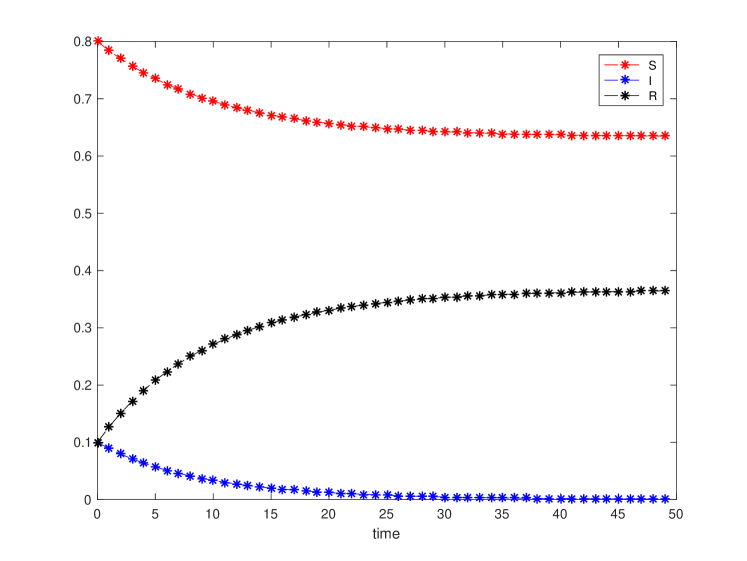
(a) $b=0.2<0.3=c$

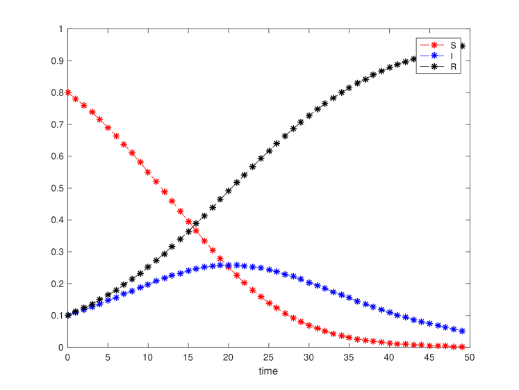
(b) $b=0.2>0.1=c$

Figure 4: the $x$=Susceptible ($S$), $y$=Infected ($I$), and $z$=Removed ($R$) long term behavior of Example 29.

Acknowledgement

Torres has been partially supported by FCT within CIDMA project UID/MAT/04106/2019, and by TOCCATA FCT project PTDC/EEI-AUT/2933/2014. The authors are very grateful to three anonymous reviewers for several constructive comments, questions and suggestions, which helped them to improve the paper.

References

- [1] N. T. J. Bailey, The mathematical theory of infectious diseases and its applications. Hafner Press [Macmillan Publishing Co., Inc.] New York, second ed., 1975.
- [2] M. Y. Li, J. R. Graef, L. Wang, and J. Karsai, “Global dynamics of a SEIR model with varying total population size,” Math. Biosci., vol. 160, no. 2, pp. 191–213, 1999.
- [3] W. R. Derrick and P. van den Driessche, “A disease transmission model in a nonconstant population,” J. Math. Biol., vol. 31, no. 5, pp. 495–512, 1993.
- [4] A. Rachah and D. F. M. Torres, “Analysis, simulation and optimal control of a SEIR model for Ebola virus with demographic effects,” Commun. Fac. Sci. Univ. Ank. Sér. A1 Math. Stat., vol. 67, no. 1, pp. 179–197, 2018. arXiv:1705.01079
- [5] N. T. J. Bailey, “Spatial models in the epidemiology of infectious diseases,” in Biological growth and spread (Proc. Conf., Heidelberg, 1979), vol. 38 of Lecture Notes in Biomath., pp. 233–261, Springer, Berlin-New York, 1980.
- [6] J. Arino, R. Jordan, and P. van den Driessche, “Quarantine in a multi-species epidemic model with spatial dynamics,” Math. Biosci., vol. 206, no. 1, pp. 46–60, 2007.
- [7] R. Rifhat, L. Wang, and Z. Teng, “Dynamics for a class of stochastic SIS epidemic models with nonlinear incidence and periodic coefficients,” Phys. A, vol. 481, pp. 176–190, 2017.
- [8] C. Yuan, D. Jiang, D. O’Regan, and R. P. Agarwal, “Stochastically asymptotically stability of the multi-group SEIR and SIR models with random perturbation,” Commun. Nonlinear Sci. Numer. Simul., vol. 17, no. 6, pp. 2501–2516, 2012.
- [9] K. Fan, Y. Zhang, S. Gao, and X. Wei, “A class of stochastic delayed SIR epidemic models with generalized nonlinear incidence rate and temporary immunity,” Phys. A, vol. 481, pp. 198–208, 2017.
- [10] J. Djordjevic, C. J. Silva, and D. F. M. Torres, “A stochastic SICA epidemic model for HIV transmission,” Appl. Math. Lett., vol. 84, pp. 168–175, 2018. arXiv:1805.01425
- [11] W. Gleissner, “The spread of epidemics,” Appl. Math. Comput., vol. 27, no. 2, pp. 167–171, 1988.
- [12] M. Bohner and A. Peterson, Dynamic equations on time scales. Boston, MA: Birkhäuser Boston Inc., 2001.
- [13] M. Bohner and A. Peterson, eds., Advances in dynamic equations on time scales. Birkhäuser Boston, Inc., Boston, MA, 2003.
- [14] M. Bohner, G. S. Guseinov, and B. Karpuz, “Properties of the Laplace transform on time scales with arbitrary graininess,” Integral Transforms Spec. Funct., vol. 22, no. 11, pp. 785–800, 2011.
- [15] M. Bohner, “Some oscillation criteria for first order delay dynamic equations,” Far East J. Appl. Math., vol. 18, no. 3, pp. 289–304, 2005.