Li Ma1ma@hiskp.uni-bonn.deQian Wang1,2wangqian@hiskp.uni-bonn.deUlf-G. Meißner1,3,4meissner@hiskp.uni-bonn.de1Helmholtz-Institut für Strahlen- und Kernphysik and Bethe Center for Theoretical Physics, Universität Bonn, D-53115 Bonn, Germany
2Institute of Quantum Matter, South China Normal University, Guangzhou 510006, China
3Institut für Kernphysik, Institute for Advanced Simulation, and Jülich Center for Hadron Physics, Forschungszentrum Jülich, D-52425 Jülich, Germany
4Tbilisi State University, 0186 Tbilisi, Georgia
Abstract
During the last decades, numerous exotic states which cannot be explained by the conventional quark model
have been observed in experiment. Some of them can be understood as two-body hadronic molecules,
such as the famous , analogous to deuteron in nuclear physics.
Along the same line, the existence of the triton leaves an open question
whether there is a bound state formed by three hadrons.
Since, for a given potential, a system with large reduced masses is more easier to form a bound state,
we study the system with the one-pion exchange potential as an exploratory
step by solving the three-body Schrödinger Equation.
We predict that a tri-meson molecular state for the system is probably
existent as long as the molecular states of its two-body subsystem exist.
As discussed above, the OPEP plays an important role in binding the two-hadron system.
From another point of view,
one can view it as a pion shared by the two constituents and form a bound state.
It can be regarded as a bond similar to the in hydrogen molecules.
There is another kind of bond called delocalized universally existing in benzene molecules,
which is a pair of electrons shared by the six carbon atoms.
A simple extension is replacing the carbon atoms by hadrons.
We have studied the role of the delocalized in forming the
three-body bound state for the double heavy tri-meson systems,
i.e. , , and
Ma:2017ery , based on the sufficient information of it sub two-body system
and the Born-Oppenheimer Approximation (BOA) which works well for a system with
several heavy and light particles Moroz:2014eba .
The crucial idea is to use Born-Oppenheimer (BO) potential for considering the influence
of the light part on the dynamics of the heavy part.
Therefore, it is a fascinating idea whether
the delocalized and the BOA could be applied to a three-heavy system,
such as the system with large reduced mass.
The same three bottomed meson system has been studied in Ref. Wilbring:2017fwy
by calculating the scattering amplitudes between the or the
and the bottomed meson. The universal bound states of three bottomed mesons from the Efimov
effect has been ruled out.
As in their calculation, only the contact interaction is included which might be the reason why
they do not find a bound state.
After including the long-range OPEP, the case might be different. Thus we solve the
three-body Schrödinger equation to discuss the system by considering the OPEP.
Without an assumption about its two-body subsystem, i.e. the molecular nature of
the or , we focus on the three-body bound state as a function of
the binding energy of its
subsystem. Hopefully, the present extensive investigations will be
useful to deepen our the understanding of a system made of three heavy particles.
This paper is organized as follows. After the introduction, the formalism and the inputs for the
system are presented in Sec. II. The dynamics of the two-body subsystem and the
corresponding BO potential are given in Sec. III and Sec. IV, respectively.
By constructing a proper interpolating wave functions for the in Sec. V,
we solve the three-body Schrödinger equation in Sec. VI. Numerical results and
discussions are given in the following section. The summary is presented in the last section.
Some technicalities are relegated to the appendix.
II Formalism and the inputs
The BOA has been successfully used in few-body system with several heavy and light
particles Braaten:2014qka ; Moroz:2014eba .
For a three-body system with one light and two heavy mesons, such as the Ma:2017ery system,
the three-body Schrödinger equation is divided into two sub equations, one is the motion of
light meson with two static sources
and the other one is
the equation for the two heavy mesons with the BO potential Ma:2017ery ,
which reflects the influence of the light meson on the dynamics of the two heavy mesons.
If the interaction between the light meson and the heavy meson is attractive,
it would make the two heavy mesons come closer, thus facilitating the formation of a bound state of
the whole system.
However, for a three heavy meson system, although the application of BOA is not straightforward,
one can employ the
underlying permutation symmetry, which means the corresponding
dynamics is invariant under the interchange of any two constituents,
for the system and continue to use the BOA for the calculation.
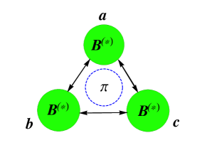
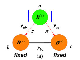
The OPEP indicates that there is only one virtual pion exchanged by any two constituents as shown
in Fig. 1.
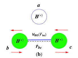
Figure 1: Dynamical illustration of the system with a circle describing the
delocalized inside. Since the three constituents have the same probabilities
to be the and , one can rewrite the system as .
One can use , and to label the three mesons in the original channel, i.e. .
It changes into via one-pion exchange (OPE) between and , and
the channel changes into through the OPE
between and . When the virtual pion arises between and ,
it returns back into the original channel .
Within this scenario, the virtual pion is not localized between any two constituents but
rather shared by the whole system.
It is very similar with the benzene molecule which has a pair of electrons shared by the
six carbon atoms, which is called in molecular physics.
Since the three constituents have the same probability to be the and mesons,
one can write the system as .
Furthermore, the order of the , and labels of the three mesons is artificial,
as the system is invariant under the interchange of the , and .
This interchange symmetry will help to simplify our calculations.
The point is that one can count the influence of each heavy meson on the
dynamics of the other two mesons one by one.
In other words, we can divide the system into three two-body subsystems , and .
In each subsystem, one should add the BO potential from the remaining one.
The existence of a negative common eigenvalue for the three subsystems may
partly answer whether there is three-body bound state for the three heavy system.
For simplicity, we call this method as ().
Before performing the calculation, we define the isospin wave functions of the
systems as with the isospin of the sub- system.
and represent the total isospin of the three-body system and its direction, respectively.
One thus obtains the isospin wave functions of the system,
Since can couple with via OPE, the coupled channel
effect is not negligible. We only consider the next close channel in our calculation.
If we distinguish the specific locations of the constituents as , and ,
there are six channels in total, i.e. , , ,
, and .
The Lagrangians with SU(2) chiral symmetry (we only consider OPE) and C-parity conservation read
(1)
(2)
where the heavy flavor meson fields and represent , , respectively. Its corresponding heavy anti-meson fields
and represent
,
.
is the pion matrix
(5)
We use the pion decay constant Zhao:2014gqa .
The pionic coupling constant is extracted from the width of
by assuming heavy quark flavor symmetryPatrignani:2016xqp .
All the parameters and input datas are listed in Table 1.
Here, we neglect isospin breaking effect and use the masses of their
charged particles.
Table 1: The coupling constants and meson masses in our calculation. The meson masses are taken
from the PDG Patrignani:2016xqp
mass(MeV)
coupling constants
MeV
Under SU(2) chiral symmetry, the OPE interaction is of order for the three-body
system. In this paper, we only take into account the OPEP to the order.
Thus, there are four kinds of effective potentials. We use to denote the effective
potential for the interaction . and denote
the process and its reverse, respectively.
represents diagonal process .
Since the interactions are physical, the effective potentials should be unitary which
gives . is used to denote the relative displacement between
the -th and -th particles.
Thus, the effective potentials of the three-body system in the channel space take the following form,
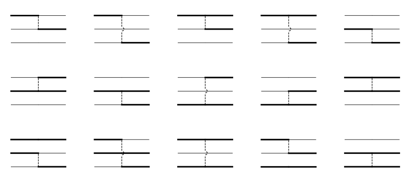
Figure 2: The leading order OPE diagrams for the transitions among the relevant three-body
channels, i.e. , , , ,
and . The solid and bold solid lines represent
the and meson fields, respectively.
Dotted lines represent pion fields.
III The break-up state and two-body subsystem
For the three bottomed meson system, suppose one of the constituent is infinitely
away from the remaining two mesons. The system can be divided into a two-body subsystem plus a free meson.
A bound state solution of the two-body subsystem indicates
a break-up state for the three-body system, i.e. a two-body bound state plus a free meson.
In the OPE model, as there is no direct interaction between two mesons,
one could expect a break-up state with the subsystem with quantum number
and a free meson .
We can detach the subsystem first, and explore its binding solution. The
Hamiltonian of the subsystem in the channel space
reads
(19)
where the and
are the relative kinetic energy for the and in their center-of-mass frame,
respectively, with , , . Here
is the angular momentum operator between meson and .
We also have the mass gap .
The effective potentials , , and depend on the isospin of the specific channels,
thus we rewrite the wave functions with fixed isospin
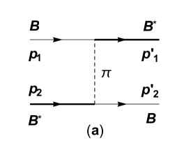
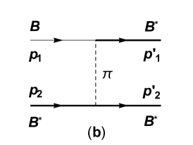
Figure 3: The u-channel Feynman diagrams for describing both the
and system’s interaction at tree level.
The regular and bold lines stand for the and the fields,
respectively. The dotted lines denote the pion fields.
For the specific channels , and , the Schrödinger equation in
the channel space takes the form
Based on this, we can derive the scattering amplitude at the tree level
(21)
where the -matrix is the interaction part of the -matrix and the is
defined as the invariant matrix element. In the second equation
we have applied the first order of Born series expansion
on the Lippmann-Schwinger equation with being the effective potential.
The relation between the scattering amplitude
and the potential is
(22)
where and denote the four-momentum and the mass of the final (initial)
state.
In the calculation, and
denote the four-momenta of the initial state particles in the center-of-mass
system shown in Fig. 3, while and
denote the four-momenta of the final state particles, respectively.
is the transferred four-momentum. For convenience, we always use
and
instead of and in the calculations.
The effective potential in coordinate space can be derived by Fourier transformation
To take into account in a rough way the substructure of each vertex,
a monopole form factor
(23)
with the pion mass and
(24)
is used to suppress the contribution from UV energies.
Here, and .
As the parameter is related to non-perturbative QCD,
it cannot be well determined. Here we only explore its effect on the binding energy
of the with the quantum number system.
To solve the time-independent
Schrödinger equation in coordinate space, the potential in momentum space
can be transformed in to that in coordinate space as shown in the Appendix.
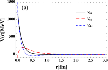
Figure 4: The effective potentials of the system
with quantum number , where (a) and (b)
correspond to the isospin and cases, respectively.
The and are the effective potentials for the S-wave and D-wave.
The represents the effective potential of S-D wave mixing.
For illustration, the value is used for the parameter .
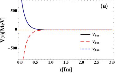
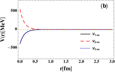
Figure 5: The effective potentials for the S-wave of the system with quantum number
, where (a) and (b) correspond to the isospin and cases, respectively.
The , and are the effective potentials
, and
for the S-wave respectively. For illustration, the
value is used for the parameter .
The isosinglet and isotriplet potentials in coordinate
space are shown in Fig. 4 (a)
and (b), respectively, with .
The isosinglet potential is repulsive which does not indicate a
bound solution. Nevertheless, the potential for the
isosinglet is attractive as shown in Fig. 5. So there is still the
possibility of a binding solution. On the contrary, the isotriplet potential
is
attractive, while its potential is repulsive. These
potentials in coordinate space can be expressed as
(25)
(26)
(27)
with . The tensor operator has the form
with the polarization vector of .
The are channel dependent coefficients, summarized in Table 2.
The in Table 2 represents the C-parity of the corresponding channel.
Table 2: Channel dependent coefficients. Here, denotes the C-parity of the two-body system.
channel
isospin
channel
Since the tensor operator leads to S-D wave mixing,
the contributions from D-wave should be taken into account. Thus the wave function
has two parts
(28)
with and the -wave and
-wave functions, respectively. In the matrix method, we use
Laguerre polynomials
(29)
as a set of orthogonal basis with the normalization condition
(30)
Thus the total wave function can be expanded as
where and are the angular part of the spin and
orbital wave function for the -wave () and -wave () states, respectively.
and are the corresponding expansion coefficients of S-wave and
D-wave, respectively. After solving the coupled-channel Schrödinger equation with the S-D wave mixing,
we obtain the binding energy and its corresponding wave function
for a given parameter . Thus the wave function has the form
(31)
Here, the wave function is normalized.
If we choose the value of the parameter MeV for instance,
one finds a loosely bound state for the isospin triplet system with a binding energy of 5.08 MeV,
when the quantum number is . There is also a loosely bound state for the isospin singlet
system, when the quantum number is . If the value of the parameter is chosen at MeV,
the isospin singlet and triplet systems have the same binding energy of 5.08 MeV. The
dependence of the binding energy on the parameter will
be given in Tables 4-5 and discussed in Sec. VII.
IV Born-Oppenheimer potential
As discussed in Sec. II, the BO potential reflects the influence of one of the mesons on
the dynamics of the other two.
For the (labeled as , and ) system,
one can derive the BO potential from for the system.
The procedure is divided into the following three steps:
•
Considering that the particle and are static with the separation ,
one can separate the degree of freedom of from the three-body system.
•
We assume the distance is a parameter. The mesons and are static,
and have one-pion interactions with meson , which can be viewed as two static sources.
•
We explore the dynamics for the meson in the limit , and subtract the
binding energy for the break-up state which is trivial for the three-body bound state.
Within this scheme, we divide the motion of the system into two parts, one is the motion of the meson
relative to the mesons and . The other one is the relative motion between mesons and
in the presence of the BO potential from .
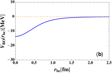
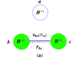
Figure 6: Illustration of the BO potential. (a) illustrates the calculation procedure of
the BO potential. (b) represents the role of the BO potential from the meson on
the dynamics of the two-body system.
As illustrated in Figs. 6, we use to denote the relative displacement
between and . Further, and represent the displacement
of the meson relative to the meson and , respectively.
One can separate the effective potentials for the meson
in Eq. (12) is the potential between .
As discussed in the previous section, one can obtain the two-body binding energy
(52)
(53)
The and in the above equation are the eigenstate
wave functions in Eq. (31).
In OPE model, as the virtual pion can only be exchanged between two of the subsystems,
the wave function of can be either
with pion exchanged between and or
with pion
exchanged between and .
The final wave function for the meson should be the superposition
of these two components
(54)
For simplicity, we neglect the mass difference for the and in the kinetic operator,
i.e. .
Then the Hamiltonian of the meson is
(61)
Accordingly, one can obtain the energy eigenvalue of the meson
where in the second step Eq. (53) and the symmetry
between and are used. Since both the two-body energy eigenvalue and the wave functions ,
depend on the parameter ,
is also a function of .
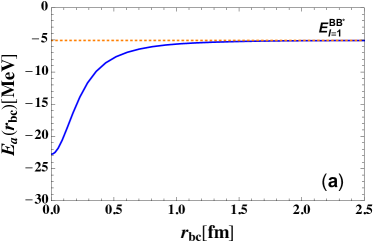
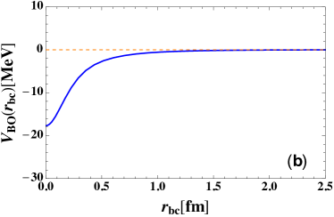
Figure 7: The energy eigenvalue of the meson and its corresponding BO potential for the
isospin triplet of the system. (a) gives the energy eigenvalue of the meson . When
, tends to the two-body energy eigenvalue , i.e. the
energy eigenvalue of the break-up state. The right panel gives the BO potential .
Here we chose the parameter MeV.
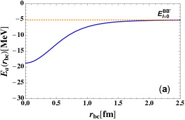
Figure 8: The energy eigenvalue of the meson and its corrsponding BO potential for the
isospin singlet of the system. (a) is the energy eigenvalue of the meson .
When , tends to the two-body energy eigenvalue , i.e.
the energy eigenvalue of the break-up state. The right panel gives the BO potential .
Here we chose the parameter MeV.
We take the parameter MeV as an example and plot for the isospin triplet
of the system in Figs. 7(a). As shown in the figure,
the energy of the meson has a minimum MeV when ,
which corresponds to the limit that the mesons and are on top of each other
and the system is reduced to the - quasi-two-body system.
When , then tends to the two-body energy eigenvalue , i.e. MeV.
This corresponds to the situation that the meson is infinitely far away from the meson .
Then the meson can only form a two-body bound state with either or .
It is not a three-body bound state anymore, but rather a two-body bound state plus a free meson state.
In fact, this is nothing but the break-up state that we have discussed in the earlier sections.
We also plot for the isospin triplet of the system in Fig. 8(a), taking
the parameter MeV. Similarly to the above,
tends to the two-body energy eigenvalue MeV.
Therefore, we should subtract the limiting value when investigating the three-body bound
state for the system.
We define the BO potential as
(62)
In other words, the BO potential between and is the energy eigenvalue
of the meson relative to that of the break-up state.
V The configurations of the three-body systems
In the OPE model, there is only one pion exchanged between any two constituents in the system.
The constituents will change themselves from vector mesons into pseudo-scalar mesons or vice verse
when they exchange one pion. Each constituent has the same probability to be a vector meson or a
pseudo-scalar meson.
Thus, the symbol is shared among them. Since only one virtual pion occurs in the
molecule, the virtual pion also be shared by the three mesons.
We can thus write the as .
The BO potential can describe the contribution for the one meson on the dynamics of the two remaining
mesons as we have discussed in the last section. Assuming that the meson and are much heavier
than the meson , then we can use the Born-Oppenheimer approximation to separate the degree of freedom
of from the three-body system. In other words, it is a kind of an adiabatic approximation that
we divide the degrees of freedom of the three-body system into a light one and a heavy one. The motion
of the light degree of freedom is the motion of meson relative to the three-body centre of mass.
The motion of the heavy degree of freedom is the relative motion between meson and . When
exploring the dynamics for the meson , we can assume the meson and are static with the
distance . Then the three-body system can be simplified as a two-body system consisting of mesons
and but with an additional BO potential generated by the meson . Overall, only the meson
can be separated from the system due to the fact that this meson is much lighter than the other ones.
A separation in this way can be a good approximation for this system.
With the same procedure that we derived Eq. (54), we obtain the wave functions
for the meson . The remaining degree of freedom is the
relative motion between meson and that can be described by a wave function assumed as
, to be determined from the Schrödinger equation. Then the total wave function of
the system then has the form
Nevertheless, the true system is that the three mesons have
little mass difference. Every meson can be considered to be a lighter one and separated from the
three-body system. Thus, the system has the three basic simplification schemes. That is
we can divide the system into three kinds of two-body
subsystems, i.e., with the BO potential created by the meson ,
with the BO potential created by the meson and
with the BO potential created by the meson as shown in Figs. 9.
These three simplification schemes can be regarded as three kinds of basic configurations.
The eigenstates of the three-body system should be combinations of them. As the most simplest
combination, one might expect the three-body eigenstate should be the superposition of the
three kinds of basic configurations.
We use the , , to denote these
three configurations. The configuration wave function represent the configuration
that we omit the meson and add the corresponding BO potential instead.
Similarly, , denote the configurations
with the BO potentials provided by the mesons and , respectively.
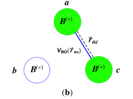
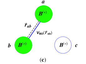
Figure 9: Three configurations of the system. (a), (b) and (c) correspond to the wave
functions , and , respectively.
Taking the configuration function as an example,
we separate the motion of the relative to the other mesons
and where their relative displacement is regarded as
a parameter as shown in Fig. 9(a).
The wave function of the has been discussed in the
last section and can be written as .
The remaining degree of freedom is the relative motion between and , which can
be taken as . Thus we have the configuration function .
The other two wave functions and can be obtained analogously,
i.e. , which correspond to the Fig. 9(b)
and Fig. 9(c), respectively.
If we regard the three configuration functions as a set of basis states, then the basis
constitute a configuration space .
The three-body eigenstate expressed as a superposition of the three kinds of basic configurations can
be described as a state vector in this configuration space.
Thus, as an interpolating wave function, the three-body wave functions can be written as
(66)
where the , and are undetermined
functions that need to be solved. The , and are the expansion coefficients.
According to Eq. (54), we rewrite the three basic configuration functions in the channel
space as
(85)
which can be expanded as a set of Laguerre polynomials
Here the subscript is the order of Laguerre polynomials. We define the order of the
configuration functions as ,
and . Further, is a normalisation constant.
We expect the three-body bound state that we seek for can be expressed as a state vector in the
configuration space .
However, the configuration functions in Eq. (66) are not an orthogonal basis.
Thus we orthonormalize the
into a new basis .
We use , and to
denote the th order of the new configuration functions ,
and , respectively. Then we have
where the is a parameter matrix which will be determined later. The are normalization
coefficients. The parameter matrix in the three configuration functions are the same due
to the interchange symmetry for the system.
Since the order configuration function should be orthogonal
with the any order of the other configuration function , one can gets
the orthogonalization condition
which gives
(86)
This equation will determine the parameter matrix . Considering the normalization of the
order configuration function
one can obtain the normalization equation for the as
(87)
After solving the equations for and , we obtain an orthonormalized configuration basis.
This basis constitutes a orthonormalized configuration space.
Then the eigenvector for the three-body system can
be written as a vector in the configuration space . Therefore, we have
where the , and are the order
expansion coefficients.
VI Three-body Schrödinger equation
As we have discussed in previous sections, if the three-body binding energy is below
the break-up threshold, the three-body system will disintegrate into a two-body system and a free meson.
Since we only focus on the three-body bound state, we could make an energy shift and remove
the energy eigenvalue for the break-up state and define a reduced Hamiltonian for
the three-body system as
The explicit form of is
(94)
where , , , , ,
are the kinetic energy operators and the corresponding reduced masses are , ,
, , ,
.
Here and
with . is the direction of the meson relative to the meson .
is the angular momentum operator between mesons and .
is the relative angular momentum operator between two-body centre of mass
for the meson and the meson .
The mass gap is .
The total Hamiltonian for the three-body system in the configuration space can be written as
(107)
with
.
The total reduced Hamiltonian for the three-body system in
the configuration space can be expressed as
(111)
with . Thus we have
The matrix element of the can be written as
(112)
where, in the last step, the interchange symmetry in the system is used.
Similarly, we also have
(113)
There are two independent matrices
to be determined,
where we have used the abbreviations , , , ,
, for , , ,
, , respectively.
The expression for the can be easily obtained by the
replacement on the expression for the
. Similarly, the expression for the
is obtained by the replacement on the expression for the . In fact,
interchange invariance for the system can simplify the calculation,
i.e.
and .
Based on the above discussion, the three-body Schrödinger equation can finally be written as
(123)
where the energy eigenvalue is the reduced three-body energy eigenvalue. The total energy
eigenvalue relative to the mass threshold is .
Solving the three-body Schrödinger equation may partly answer whether the
three-body system has a loosely bound state or not.
VII Application to the system
In order to verify the feasibility of the Born-Oppenheimer potential method for the three heavy system, we apply it to the three nucleon system.
Since there is sufficient experimental data for this
system, we can apply the formalism introduced above
to investigate its binding energy and illustrate the
feasibility of our formalism.
As we know, the triton and the helium-3 (3He) nucleus are the two possible bound states of the system,
both of them have the quantum numbers but have different isospin on its direction.
They have the same structure and the binding energy if isospin symmetry breaking effect is neglected.
The calculation on the three-nucleon system is much more straightforward than the system, as there are no other
coupled channels. For simplicity, we only write down the isospin wave functions of the triton and helium-3 nuclei, which are
The Lagrangian reads
where the is the coupling constants (we use here the pseudoscalar coupling, which is fine to the order we are
working, see e.g. Ref. Bernard:1989fe ). is the nucleon doublet. Further, are the Pauli matrices, and are the fields.
With a procedure similar to the one discussed in the Sec. II-VI, we can investigate the properties of the
break-up state formed by a deuteron and a free nucleon as well as the three-body bound states.
As discussed in the above sections, there is only one free parameter in the
monopole form factor introduced in Sec. III,
which reflects, in a rough way, the internal structure of the interacting hadrons. In other words,
the size of hadron is proportional to , which is still unknown from the fundamental theory.
Thus the parameter
is fixed by the binding energy MeV of
deuteron in our calculations. With the so determined parameter , we can obtain the BO potentials for the
system using the formalism in the Sec. II-VI, with just the replacement of the effective potential
by in the calculations. This potential reads
where the is the channel-dependent coefficient for the two-nucleon system, is the mass of nucleon,
is the pion-nucleon coupling constant, and and are the spin Pauli matrix
for the nucleon 1 and 2 in the scattering process .
Table 3: Bound state solutions of the system with isospin .
is the energy eigenvalue of its subsystem.
is the reduced three-body energy eigenvalue relative to the break-up state of the system.
is the total three-body energy eigenvalue relative to the threshold.
is the minimum of the BO potential.
represents the root-mean-square radius of any two in the system.
The -wave and -wave represent the probabilities for -wave and
-wave components in any two in the system.
(MeV)
(MeV)
(MeV)
(MeV)
(MeV)
S wave(%)
D wave(%)
(fm)
830.00
-0.18
-1.93
-2.11
-4.54
94.01
5.99
4.21
850.00
-0.67
-2.71
-3.38
-5.36
93.36
6.64
4.00
870.00
-1.23
-3.65
-4.88
-6.32
92.68
7.32
3.78
890.00
-1.88
-4.77
-6.66
-7.42
91.99
8.01
3.54
899.60
-2.23
-5.38
-7.62
-8.00
91.66
8.34
3.42
900.00
-2.25
-5.41
-7.66
-8.03
91.64
8.36
3.42
920.00
-3.05
-6.85
-9.90
-9.35
90.97
9.03
3.18
940.00
-3.98
-8.51
-12.49
-10.83
90.35
9.65
2.95
960.00
-5.03
-10.42
-15.45
-12.46
89.76
10.24
2.74
980.00
-6.21
-12.57
-18.78
-14.23
89.23
10.77
2.54
1000.00
-7.55
-14.97
-22.51
-16.14
88.73
11.27
2.37
1020.00
-9.04
-17.61
-26.65
-18.19
88.27
11.73
2.23
1040.00
-10.69
-20.51
-31.20
-20.37
87.84
12.16
2.10
After solving the three-body Schrödinger equation, i.e.Eq. (123), one can obtain
the dependence of the binding of the three-nucleon system on the parameter
(Table 3). As shown in the table, there is a three-body bound
state with the reduced binding energy and the total three-body bound energy
in the range of - and - , respectively,
when the parameter varies from to .
The corresponding isospin singlet two-body subsystem has the
binding enrgy in the range of - .
The root-mean-square of the system decreases from
4.21 to 2.10 when the parameter increases.
Once the parameter fixed by the deuteron
binding energy, the reduced three-body binding energy and the total binding
energy relative to the three free nucleons are 5.38 and
7.62 , respectively. The later is comparable with the
empirical binding energies of the triton (8.48 ) and helium-3 (7.80 ) nuclei.
Noet again that there is no numerical difference between the binding energies of triton
and helium-3 in the calculation, as the isospin breaking has not be considered.
For a better illustration of the binding property,
we plot the dependence of the reduced three-body binding energy
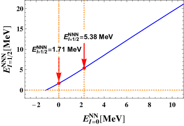
on the two-body binding energy of its deuteron subsystem.
As shown in Fig. 10, the binding energy of the three-nucleon system
becomes larger when the binding energy of its subsystem increases.
There are two red points in the figure,
the left red point is the critical point which indicates
the lower limit of the required binding energy of the deuteron
to form a three-body bound state. It is very interesting that
even though the binding energy of its subsystem is zero,
there is a small binding energy of the three-nucleon system, which is 1.71 .
This is reminsicent of a Borromean state,
where a three-body system may have a bound state despite the fact that none of its subsystems forms a bound state.
The other red point is our numerical result of the binding energy of triton or helium-3. It is a little below the experimental
values since in our calculations we use the BOP method to construct our interpolating wave functions, which can be regarded as
a version of the variational principle. As we know, this always give an upper limit of the energy of a system.
Figure 10: Dependence of the reduced three-body binding energy on the binding energy of
its two-body subsystem (the deuteron).
The left red point is the critical point which indicates the lower
limit of the required binding energy of the deuteron to form a three-body bound state. The right
one is our numerical result of the binding energy of the triton or the helium-3 nucleus.
VIII Numerical results on the system
The application of the BOP method to the three-nucleon system has verified its feasibility to some extent. Now we return to the system mainly discussed in this paper, i.e. the three mesons system .
There is only one free parameter in the monopole form factor which is undetermined in our calculations.
For the deuteron case, the parameter is within the range .
One would expect that the size of heavier bottom system is smaller than the size of deuteron,
leading to a larger . Thus, we vary the parameter from
to to study whether the system is bound or not.
In order to show the properties of the two-body interactions for the , we first present
the numerical results for the break-up state in Tables 4-5. We plot
the effective potentials for the in Fig. 4 and Fig. 5,
where the regularization parameter is fixed at 1440 MeV. In these figures, (a) and (b) correspond
to the isospin and cases, respectively. After carefully solving the coupled-channel
Schrödinger equation with the treatment of the S-D wave mixing, we find loosely bound
states for both cases.
For the isospin triplet case, i.e. , the dependence of
the binding energy of the two-body system on the regularization parameter
is shown in Table 4. The energy threshold of the break-up state
for the is just the two-body energy eigenvalue of the plus the mass of the three
static free meson. We use denote the energy eigenvalue of the .
When the parameter varies from to ,
there is a bound state solution with the binding energy
and the root-mean-square radius . The -wave component takes over
comparing to the value for -wave.
The and channels have probabilities
and , respectively. The proportion of the channel and D-wave component
are relatively small. However, as the value of the regularization parameter increases,
the and interacting with pion is more like a point particle, the proportion of
the channel increases greatly, while the D-wave component decreases.
We plot the radial wave functions of the -wave and -wave
Fig. 11(a) for the system , obviously, the bound state we have
found is ground state.
Table 4: Bound state solutions of the system with the isospin . is the
parameter in the form factor. is the energy eigenvalue. The binding energy is .
is the root-mean-square radius. and are the probabilities for the
components and , respectively.
Proportion
(MeV)
(MeV)
S wave(%)
D wave(%)
S wave(%)
D wave(%)
(fm)
(%)
(%)
1380
-2.11
99.13
0.87
99.21
0.79
1.51
91.91
8.09
1400
-2.94
99.12
0.88
99.36
0.64
1.30
90.22
9.78
1420
-3.93
99.14
0.86
99.49
0.51
1.15
88.47
11.53
1440
-5.08
99.16
0.84
99.59
0.41
1.03
86.69
13.31
1460
-6.40
99.19
0.81
99.68
0.33
0.94
84.91
15.09
1480
-7.88
99.22
0.78
99.74
0.26
0.86
83.14
16.86
1500
-9.54
99.25
0.75
99.80
0.20
0.80
81.40
18.60
1520
-11.38
99.29
0.71
99.84
0.16
0.75
79.70
20.30
1540
-13.39
99.32
0.68
99.88
0.12
0.71
78.07
21.93
1560
-15.59
99.36
0.64
99.91
0.09
0.67
76.50
23.50
For the isospin singlet case, i.e. , the dependence of
the binding energy of the two-body system on the regularization parameter
is shown in Table 5. We also use to denote the energy eigenvalue of the .
When the parameter varies from to ,
there is a bound state solution with binding energy
and the root-mean-square radius . The -wave component is
compared to the value for -wave.
The and channels have probabilities
and , respectively. The proportion of the channel and D-wave component are
relatively small which is similar with the case of isospin triplet. As the value of the
regularization parameter increases, the proportion of the channel increases greatly.
Different from the case of isospin triplet the S-wave component decrease and D-wave increase as
increases. As the parameter increases, all of the effective potentials become
stronger. The S-wave potential increases faster than the D-wave potential for the isospin triplet case,
while it is reverse for the isospin singlet case.
In order to check whether the bound state we have found is the ground state, we also plot the radial
wave functions of the -wave and -wave Fig. 11(b) for the system .
Table 5: Bound state solutios of the with the isospin . is the
parameter in the form factor. is the energy eigenvalue. The binding energy is .
is the root-mean-square radius. and are the probabilities for the
component and , respectively.
Proportion
(MeV)
(MeV)
S wave(%)
D wave(%)
S wave(%)
D wave(%)
(fm)
(%)
(%)
1040
-1.88
86.09
13.91
68.84
31.16
2.03
92.05
7.95
1060
-2.63
84.59
15.41
69.41
30.59
1.79
90.18
9.82
1080
-3.54
83.26
16.74
69.90
30.10
1.60
88.22
11.78
1100
-4.62
82.07
17.93
70.33
29.67
1.45
86.22
13.78
1120
-5.87
81.01
18.99
70.69
29.31
1.33
84.22
15.78
1140
-7.29
80.07
19.93
70.99
29.01
1.23
82.25
17.75
1160
-8.89
79.23
20.77
71.25
28.75
1.14
80.34
19.66
1180
-10.67
78.49
21.51
71.46
28.54
1.07
78.50
21.50
1200
-12.63
77.81
22.19
71.63
28.37
1.01
76.75
23.25
1220
-14.78
77.21
22.79
71.77
28.23
0.95
75.09
24.91
In Sec. II, we have listed the isospin wave functions of the which are expressed as
. After solving the three-body Schrödinger equation via the method
of Sec. V, we find that all of these isospin eigenstates have bound state solutions.
As long as the two-body system has a loosely bound state, the three-body system is most
likely to have a loosely bound state, too. We have collected the dependence of the three-body bound state
solutions on the two-body binding energy in Tables 6-7.
The bound state solutions for the state are
shown in Table 6. The three-body binding energy relative to their break-up states is 5.67 MeV,
when the parameter is chosen at 1440 MeV and the two-body binding energy of their
subsystems is 5.08 MeV. To search for the dependence on the binding energy of the two-body
system , we change the parameter . It turns out that if the value of the varies
from to , then the reduced three-body energy eigenvalue
decreases from to and the total three-body energy
eigenvalue decreases from to . The structure of the
three-body bound state is a regular triangle with the root-mean-square length of one side decreasing
from 3.98 fm to 0.65 fm. In order to illustrate the strength of the BO potential, we also collect
its minimum in the table within the range of -3.43-37.24 MeV as the increases.
As increases, the effective attraction between and becomes stronger, the BO potential
becomed deeper, so then the three-body system becomes tighter and has a larger binding energy. From
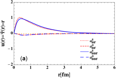
the results in the table, we can also see that the dominant wave between any two in
the is wave and the dominant channel is the instead of the
channel. For comparison, we plot the wave functions for any two in the system
and that for the two-body system in Fig. 11(a) with MeV. The shapes of
these exhibit little difference. From another perspective, one more meson has little effect
on the size of the system but greatly increases the binding energy.
Table 6: Bound state solutions of the with the isospin .
is the energy eigenvalue of its subsystem with the isospin .
is the reduced three-body energy eigenvalue relative to the break-up state of the system.
is the total three-body energy eigenvalue relative to the threshold.
is the minimum of the BO potential.
represents the root-mean-square radius of any two in the system.
The -wave and -wave represent the probabilities for -wave and
-wave components in any two in the .
The and denote the probabilities for the and components,
respectively.
(MeV)
(MeV)
(MeV)
(MeV)
S wave(%)
D wave(%)
(fm)
(%)
(%)
-0.18
-0.19
-0.38
-3.43
99.76
0.24
3.98
97.50
2.50
-0.48
-0.45
-0.93
-4.88
99.68
0.32
3.34
96.39
3.61
-0.89
-0.85
-1.74
-6.62
99.59
0.41
2.67
95.02
4.98
-1.43
-1.42
-2.85
-8.56
99.49
0.51
2.11
93.78
6.22
-2.11
-2.20
-4.31
-10.65
99.41
0.59
1.71
91.91
8.09
-2.94
-3.17
-6.11
-12.87
99.34
0.66
1.43
90.22
9.78
-3.93
-4.33
-8.26
-15.21
99.29
0.71
1.24
88.47
11.53
-5.08
-5.67
-10.75
-17.65
99.25
0.75
1.09
86.69
13.31
-6.40
-7.18
-13.58
-20.19
99.22
0.78
0.98
84.91
15.09
-7.88
-8.83
-16.71
-22.83
99.20
0.80
0.90
83.14
16.86
-9.54
-10.61
-20.16
-25.55
99.18
0.82
0.83
81.40
18.60
-11.38
-12.51
-23.89
-28.36
99.17
0.83
0.77
79.70
20.30
-13.39
-14.62
-28.01
-31.24
99.16
0.84
0.72
78.07
21.93
-15.59
-16.75
-32.34
-34.20
99.15
0.85
0.68
76.50
23.50
-17.97
-18.99
-36.95
-37.24
99.14
0.86
0.65
75.01
24.99
For the state , we also find a loosely bound solution, which
is shown in Table 7. The three-body binding energy relative to their break-up states is
7.18 MeV, when the parameter is chosen at 1107.7 MeV and the two-body binding energy of their
subsystems is 5.08 MeV. In order to show the dependence on the binding energy of the
two-body system , we also change the parameter . We find that if the value of the
varies from to , then the reduced three-body energy
eigenvalue decreases from to and the total
three-body energy eigenvalue decreases from to .
The structure of the three-body bound state is a regular triangle with the root-mean-square length
of one side decreasing from 3.89 fm to 0.93 fm. As an illustration for the strength of the BO potential,
we also list its minimum in the table within the range of 2.15 MeV as
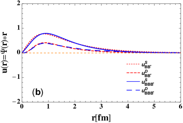
increases. Similar to the case, the dominant wave between any two
in the is wave and the dominant channel is the one. In order to show
that one more meson has little effect on the size of the system, we also plot the wave
functions for any two in the system and that for the two-body system
in Fig. 11(b) with MeV. Here we chose the parameter MeV
for a better comparison with the case,
since both cases have the same two-body binding energy 5.08 MeV.
Table 7: Bound state solutions of the with isospin .
is the energy eigenvalue of its subsystem with the isospin .
is the reduced three-body energy eigenvalue relative to the break-up state of the system.
is the total three-body energy eigenvalue relative to the threshold.
is the minimum of the BO potential.
represents the root-mean-square radius of any two in the system.
The -wave and -wave represent the probabilities for -wave and
-wave components in any two in the .
The and denote the probabilities for the and components,
respectively.
(MeV)
(MeV)
(MeV)
(MeV)
S wave(%)
D wave(%)
(fm)
(%)
(%)
-0.19
-0.32
-0.51
-2.15
94.66
5.34
3.89
97.68
2.32
-0.44
-0.64
-1.08
-3.04
92.56
7.44
3.27
96.66
3.34
-0.80
-1.13
-1.93
-4.19
90.43
9.57
2.69
95.36
4.64
-1.27
-1.82
-3.09
-5.57
88.49
11.51
2.24
93.80
6.20
-1.88
-2.72
-4.60
-7.14
86.72
13.28
1.93
92.05
7.95
-2.63
-3.82
-6.45
-8.89
85.09
14.91
1.70
90.18
9.82
-3.54
-5.11
-8.65
-10.78
83.60
16.40
1.53
88.22
11.78
-4.62
-6.57
-11.20
-12.82
82.27
17.73
1.40
86.22
13.78
-5.04
-7.13
-12.17
-13.56
81.84
18.16
1.36
85.52
14.48
-7.29
-10.00
-17.29
-17.25
80.06
19.94
1.21
82.25
17.75
-8.89
-11.93
-20.83
-19.63
79.15
20.85
1.13
80.34
19.66
-10.67
-14.00
-24.68
-22.12
78.36
21.64
1.07
78.50
21.50
-12.63
-16.20
-28.84
-24.70
77.66
22.34
1.02
76.75
23.25
-14.78
-18.52
-33.30
-27.38
77.03
22.97
0.97
75.09
24.91
-17.10
-20.96
-38.06
-30.15
76.46
23.54
0.93
73.52
26.48
The state also has a loosely bound solution. However, in
our calculation the states and are degenerate. This is due to the fact that in the OPE model
only two-body interactions are considered, and the two-body interaction is only depends on the
total isospin of the two interacting mesons. The states and
have the same two-body interaction but
may have different three-body interaction. If we further consider the calculation to the
next-to-next leading order, this degeneracy may disappear. The calculation that contains three-body
interactions via pion exchange is quite complicated, which is left for the further work.
The numerical results show that the three-body binding energy increases as the two-body
binding energy increases. One may wonder whether there is a critical value of the , below which
the three-body system has no bound state solution.
After lots of calculations, it turns out that all of the isospin eigenstates have no such critical value.
That is to say, no matter what a small value for the two-body binding energy ,
as long as the two-body system has a loosely bound state, the three-body system
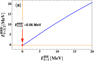
probably has a loosely bound state. To show this conclusion explicitly, we plot the dependence of
the three-body binding energy on the variety of two-body binding energy in Fig. 12.
The isospin eigenstate and cases are shown in Fig. 12(a), where and
denote the reduced three-body binding energy and two-body binding energy, respectively.
When the two-body binding energy approaches 0 MeV, the reduced three-body binding
energy approaches a small value of about 0.06 MeV. Similarly, we also plot the
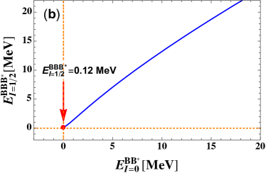
dependence curve for the case in Fig. 12(b),
where and denote the reduced three-body binding energy and
two-body binding energy in this case, respectively. As shown in the figure, the reduced
three-body binding energy also has a small value of about 0.12 MeV,
when the two-body binding energy approaches zero.
Figure 11: Plot of various wave functions. The blue lines represent the wave functions for
any two constituents in the . The red lines denote the wave functions for its
subsystem . (a) corresponds to the isospin states and cases. (b) corresponds to
the isospin state case. Here we chose the parameter
MeV in t (a) and MeV in (b) for a better comparison of
all the cases, since they have the same two-body binding energy of 5.08 MeV.
Figure 12: Dependence of the reduced three-body binding energy on the two-body binding energy of
its subsystem . The red point is the critical point which indicates the lower
limit of the required binding energy of the isotriplet to form a three-body bound state.
(a) corresponds to the isospin states
and cases, while (b) corresponds to the isospin state
case.
IX Summary and Discussion
In the present paper, we have performed an extensive study on the possibility of the system to
form tri-meson molecules. Based on the Born-Oppenheimer potential method as well as the OPE scheme,
we derived the three-body Schrödinger equation for the system . Since the
regularization parameter is difficult to be pinned down, we choose the parameter in the range of
0.91.6 GeV and show various bound state solutions of the system. After
careful treatments of the S-D wave mixing and the coupled-channel effects, we
found that all of the isospin eigenstates expressed by the have bound state solutions.
For instance, in the states and
, the three-body binding energy relative to their break-up
states is 5.67 MeV, when the parameter is chosen at 1440 MeV and the two-body binding
energy of their subsystems is 5.08 MeV. In the state ,
the three-body binding energy relative to their break-up states is 7.18 MeV, when the parameter
is chosen at 1107.7 MeV and the two-body binding energy of their subsystems is
also 5.08 MeV. After careful calculations, we find no critical value for the two-body binding energy,
which indicates the lower limit of the required binding energy of their subsystem to form
a three-body bound state. That is to say, no matter how small the two-body binding energy is,
as long as the two-body subsystem has a loosely bound state, the three-body system
is most likely to have a loosely bound state, too.
The BO potential method we have used in this paper is an adiabatic approximation that divide
the degrees of freedom of the motion for the three-body system into a light one and a heavy one.
Then we simplify the three-body system into a two-body system only with heavy degrees of freedom
but with an additional BO potential generated by the relative light meson. Since the system
has little mass difference on its constituents,
the motion of every constituent can be regarded as a light degree of freedom. Therefore, the
eigenstates of the three-body system should be the combinations of all of the possible cases.
As the most simplest combination, one might expect the three-body eigenstate should be a
superposition all of the possible cases. In other words, the three-body bound state solutions we
have listed in the last section are approximate solutions. It may be that the strict solutions will
be a more complicated combinations. To answer this question requires further study.
Our calculations are based on the OPE scheme, which is leading order in the chiral power counting
(neglecting contact interactions). Since only one virtual pion occurs in the molecule,
the virtual pion is also shared by the three mesons. Therefore, the three constituents in the
system share one virtual pion which corresponds to a delocalized pion bond.
It is attractive and strong enough to make them form a three-body molecular state.
To summarize briefly, with the delicate efforts of the long-range one-pion exchange, the S-D wave mixing
and coupled-channel effects, we have investigated the existence of the loosely bound
tri-meson molecules and find that it is very easy to form a tri-meson molecular state
as long as its two-body subsystem has a molecular state. Hopefully, the present extensive
investigations will be useful to the understanding of the few-body hadronic systems and the
future well-developed experiments on hadron collisions will provide us with a platform to seek
out the tri-meson molecules.
Acknowledgements
This work is
supported in part by the DFG (Grant No. TRR110) and the NSFC (Grant No. 11621131001) through funds
provided to
the Sino-German CRC 110 “Symmetries and the Emergence of Structure
in QCD”. The work of UGM was also supported by the Chinese Academy
of Sciences (CAS) President’s International Fellowship Initiative (PIFI)
(Grant No. 2018DM0034) and by VolkswagenStiftung (Grant No. 93562).
QW is also supported by the Thousand Talents Plan for Young Professionals and
research startup funding at SCNU.
Appendix: Some helpful functions and Fourier transformations
The functions and in Eqs. (25)-(27) are defined as
where
Fourier transformation formulas read
where .
The polarization vector is the S-D wave space have the following substitution
References
(1)
E. Klempt and A. Zaitsev,
Phys. Rept. 454, 1 (2007)
doi:10.1016/j.physrep.2007.07.006
[arXiv:0708.4016 [hep-ph]].
(2)
E. Klempt and J. M. Richard,
Rev. Mod. Phys. 82, 1095 (2010)
doi:10.1103/RevModPhys.82.1095
[arXiv:0901.2055 [hep-ph]].
(3)
N. Brambilla et al.,
Eur. Phys. J. C 71, 1534 (2011)
doi:10.1140/epjc/s10052-010-1534-9
[arXiv:1010.5827 [hep-ph]].
(4)
S. L. Olsen,
Front. Phys. (Beijing) 10, no. 2, 121 (2015)
doi:10.1007/S11467-014-0449-6
[arXiv:1411.7738 [hep-ex]].
(5)
E. Oset et al.,
Int. J. Mod. Phys. E 25, 1630001 (2016)
doi:10.1142/S0218301316300010
[arXiv:1601.03972 [hep-ph]].
(6)
H. X. Chen, W. Chen, X. Liu and S. L. Zhu,
Phys. Rept. 639, 1 (2016)
doi:10.1016/j.physrep.2016.05.004
[arXiv:1601.02092 [hep-ph]].
(7)
H. X. Chen, W. Chen, X. Liu, Y. R. Liu and S. L. Zhu,
Rept. Prog. Phys. 80, no. 7, 076201 (2017)
doi:10.1088/1361-6633/aa6420
[arXiv:1609.08928 [hep-ph]].
(8)
A. Esposito, A. Pilloni and A. D. Polosa,
Phys. Rept. 668, 1 (2017)
doi:10.1016/j.physrep.2016.11.002
[arXiv:1611.07920 [hep-ph]].
(9)
R. F. Lebed, R. E. Mitchell and E. S. Swanson,
Prog. Part. Nucl. Phys. 93, 143 (2017)
doi:10.1016/j.ppnp.2016.11.003
[arXiv:1610.04528 [hep-ph]].
(10)
A. Hosaka, T. Iijima, K. Miyabayashi, Y. Sakai and S. Yasui,
PTEP 2016, no. 6, 062C01 (2016)
doi:10.1093/ptep/ptw045
[arXiv:1603.09229 [hep-ph]].
(11)
Y. Dong, A. Faessler and V. E. Lyubovitskij,
Prog. Part. Nucl. Phys. 94, 282 (2017).
doi:10.1016/j.ppnp.2017.01.002
(12)
F. K. Guo, C. Hanhart, U.-G. Meißner, Q. Wang, Q. Zhao and B. S. Zou,
Rev. Mod. Phys. 90, no. 1, 015004 (2018)
doi:10.1103/RevModPhys.90.015004
[arXiv:1705.00141 [hep-ph]].
(13)
S. L. Olsen, T. Skwarnicki and D. Zieminska,
Rev. Mod. Phys. 90, no. 1, 015003 (2018)
doi:10.1103/RevModPhys.90.015003
[arXiv:1708.04012 [hep-ph]].
(14)
A. Francis, R. J. Hudspith, R. Lewis and K. Maltman,
Phys. Rev. Lett. 118, no. 14, 142001 (2017)
doi:10.1103/PhysRevLett.118.142001
[arXiv:1607.05214 [hep-lat]].
(15)
M. Karliner and J. L. Rosner,
Phys. Rev. Lett. 119, no. 20, 202001 (2017)
doi:10.1103/PhysRevLett.119.202001
[arXiv:1707.07666 [hep-ph]].
(16)
E. J. Eichten and C. Quigg,
Phys. Rev. Lett. 119, no. 20, 202002 (2017)
doi:10.1103/PhysRevLett.119.202002
[arXiv:1707.09575 [hep-ph]].
(17)
R. Machleidt, K. Holinde and C. Elster,
Phys. Rept. 149, 1 (1987).
doi:10.1016/S0370-1573(87)80002-9
(18)
N. A. Tornqvist,
hep-ph/0308277.
(19)
R. A. Malfliet and J. A. Tjon,
Nucl. Phys. A 127, 161 (1969).
doi:10.1016/0375-9474(69)90775-1
(20)
G. Eichmann, R. Alkofer, A. Krassnigg and D. Nicmorus,
Phys. Rev. Lett. 104, 201601 (2010)
doi:10.1103/PhysRevLett.104.201601
[arXiv:0912.2246 [hep-ph]].
(21)
N. Ishii, W. Bentz and K. Yazaki,
Nucl. Phys. A 587, 617 (1995).
doi:10.1016/0375-9474(95)00032-V
(22)
G. Eichmann,
Phys. Rev. D 84, 014014 (2011)
doi:10.1103/PhysRevD.84.014014
[arXiv:1104.4505 [hep-ph]].
(23)
S. z. Huang and J. Tjon,
Phys. Rev. C 49, 1702 (1994)
doi:10.1103/PhysRevC.49.1702
[hep-ph/9308362].
(24)
N. Ishii, W. Bentz and K. Yazaki,
Phys. Lett. B 301, 165 (1993).
doi:10.1016/0370-2693(93)90683-9
(25)
S. Ishikawa,
Few Body Syst. 32, 229 (2003)
doi:10.1007/s00601-003-0001-7
[nucl-th/0206064].
(26)
H. Sanchis-Alepuz, G. Eichmann, S. Villalba-Chavez and R. Alkofer,
Phys. Rev. D 84, 096003 (2011)
doi:10.1103/PhysRevD.84.096003
[arXiv:1109.0199 [hep-ph]].
(27)
C. Elster, W. Glöckle and H. Witala,
Few Body Syst. 45, 1 (2009)
doi:10.1007/s00601-008-0003-6
[arXiv:0807.1421 [nucl-th]].
(28)
G. Eichmann, I. C. Cloet, R. Alkofer, A. Krassnigg and C. D. Roberts,
Phys. Rev. C 79, 012202 (2009)
doi:10.1103/PhysRevC.79.012202
[arXiv:0810.1222 [nucl-th]].
(29)
C. Popovici, P. Watson and H. Reinhardt,
Phys. Rev. D 83, 025013 (2011)
doi:10.1103/PhysRevD.83.025013
[arXiv:1010.4254 [hep-ph]].
(30)
Y. Fujiwara, M. Kohno and Y. Suzuki,
Few Body Syst. 34, 237 (2004)
doi:10.1007/s00601-004-0021-y
[nucl-th/0310028].
(31)
A. Stadler, W. Glöckle and P. U. Sauer,
Phys. Rev. C 44, 2319 (1991).
doi:10.1103/PhysRevC.44.2319
(32)
A. Martinez Torres, K. P. Khemchandani, L. S. Geng, M. Napsuciale and E. Oset,
Phys. Rev. D 78, 074031 (2008)
doi:10.1103/PhysRevD.78.074031
[arXiv:0801.3635 [nucl-th]].
(33)
A. Martinez Torres, K. P. Khemchandani, D. Jido and A. Hosaka,
Phys. Rev. D 84, 074027 (2011)
doi:10.1103/PhysRevD.84.074027
[arXiv:1106.6101 [nucl-th]].
(34)
A. Martinez Torres, D. Jido and Y. Kanada-En’yo,
Phys. Rev. C 83, 065205 (2011)
doi:10.1103/PhysRevC.83.065205
[arXiv:1102.1505 [nucl-th]].
(35)
X. L. Ren, B. B. Malabarba, L. S. Geng, K. P. Khemchandani and A. Martínez Torres,
Phys. Lett. B 785, 112 (2018)
doi:10.1016/j.physletb.2018.08.034
[arXiv:1805.08330 [hep-ph]].
(36)
A. Martinez Torres, K. P. Khemchandani, D. Gamermann and E. Oset,
Phys. Rev. D 80, 094012 (2009)
doi:10.1103/PhysRevD.80.094012
[arXiv:0906.5333 [nucl-th]].
(37)
C. W. Xiao, M. Bayar and E. Oset,
Phys. Rev. D 84, 034037 (2011)
doi:10.1103/PhysRevD.84.034037
[arXiv:1106.0459 [hep-ph]].
(38)
J. J. Xie, A. Martinez Torres and E. Oset,
Phys. Rev. C 83, 065207 (2011)
doi:10.1103/PhysRevC.83.065207
[arXiv:1010.6164 [nucl-th]].
(39)
J. M. Dias, V. R. Debastiani, L. Roca, S. Sakai and E. Oset,
Phys. Rev. D 96, no. 9, 094007 (2017)
doi:10.1103/PhysRevD.96.094007
[arXiv:1709.01372 [hep-ph]].
(40)
D. Jido and Y. Kanada-En’yo,
Phys. Rev. C 78, 035203 (2008)
doi:10.1103/PhysRevC.78.035203
[arXiv:0806.3601 [nucl-th]].
(41)
A. Martinez Torres, K. P. Khemchandani and E. Oset,
Phys. Rev. C 79, 065207 (2009)
doi:10.1103/PhysRevC.79.065207
[arXiv:0812.2235 [nucl-th]].
(42)
M. Bayar and E. Oset,
Nucl. Phys. A 883, 57 (2012)
doi:10.1016/j.nuclphysa.2012.04.005
[arXiv:1203.5313 [nucl-th]].
(43)
E. Oset, D. Jido, T. Sekihara, A. Martinez Torres, K. P. Khemchandani, M. Bayar and J. Yamagata-Sekihara,
Nucl. Phys. A 881, 127 (2012)
doi:10.1016/j.nuclphysa.2012.02.005
[arXiv:1203.4798 [hep-ph]].
(44)
A. Martinez Torres, E. J. Garzon, E. Oset and L. R. Dai,
Phys. Rev. D 83, 116002 (2011)
doi:10.1103/PhysRevD.83.116002
[arXiv:1012.2708 [hep-ph]].
(45)
W. Liang, C. W. Xiao and E. Oset,
Phys. Rev. D 88, no. 11, 114024 (2013)
doi:10.1103/PhysRevD.88.114024
[arXiv:1309.7310 [hep-ph]].
(46)
M. Bayar, X. L. Ren and E. Oset,
Eur. Phys. J. A 51, no. 5, 61 (2015)
doi:10.1140/epja/i2015-15061-8
[arXiv:1501.02962 [hep-ph]].
(47)
J. Yamagata-Sekihara, L. Roca and E. Oset,
Phys. Rev. D 82, 094017 (2010)
Erratum: [Phys. Rev. D 85, 119905 (2012)]
doi:10.1103/PhysRevD.82.094017, 10.1103/PhysRevD.85.119905
[arXiv:1010.0525 [hep-ph]].
(48)
L. Roca and E. Oset,
Phys. Rev. D 82, 054013 (2010)
doi:10.1103/PhysRevD.82.054013
[arXiv:1005.0283 [hep-ph]].
(49)
J. J. Xie, A. Martinez Torres, E. Oset and P. Gonzalez,
Phys. Rev. C 83, 055204 (2011)
doi:10.1103/PhysRevC.83.055204
[arXiv:1101.1722 [nucl-th]].
(50)
V. R. Debastiani, J. M. Dias and E. Oset,
Phys. Rev. D 96, no. 1, 016014 (2017)
doi:10.1103/PhysRevD.96.016014
[arXiv:1705.09257 [hep-ph]].
(51)
Y. Ikeda and T. Sato,
Phys. Rev. C 76, 035203 (2007)
doi:10.1103/PhysRevC.76.035203
[arXiv:0704.1978 [nucl-th]].
(52)
C. Hajduk and P. U. Sauer,
Nucl. Phys. A 322, 329 (1979).
doi:10.1016/0375-9474(79)90429-9
(53)
Y. Ikeda and T. Sato,
Phys. Rev. C 79, 035201 (2009)
doi:10.1103/PhysRevC.79.035201
[arXiv:0809.1285 [nucl-th]].
(54)
A. Gal and H. Garcilazo,
Phys. Rev. Lett. 111, 172301 (2013)
doi:10.1103/PhysRevLett.111.172301
[arXiv:1308.2112 [nucl-th]].
(55)
K. Dreissigacker, S. Furui, C. Hajduk, P. U. Sauer and R. Machleidt,
Nucl. Phys. A 375, 334 (1981).
doi:10.1016/0375-9474(82)90018-5
(56)
S. König, H. W. Grießhammer, H. W. Hammer and U. van Kolck,
J. Phys. G 43, no. 5, 055106 (2016)
doi:10.1088/0954-3899/43/5/055106
[arXiv:1508.05085 [nucl-th]].
(57)
S. König and H. W. Hammer,
EPJ Web Conf. 113, 04011 (2016).
doi:10.1051/epjconf/201611304011
(58)
E. Wilbring, H.-W. Hammer and U.-G. Meißner,
arXiv:1705.06176 [hep-ph].
(59)
M. Schmidt, M. Jansen and H.-W. Hammer,
Phys. Rev. D 98, no. 1, 014032 (2018)
doi:10.1103/PhysRevD.98.014032
[arXiv:1804.00375 [hep-ph]].
(60)
H. W. Hammer, J. Y. Pang and A. Rusetsky,
JHEP 1709, 109 (2017)
doi:10.1007/JHEP09(2017)109
[arXiv:1706.07700 [hep-lat]].
(61)
H.-W. Hammer, J.-Y. Pang and A. Rusetsky,
JHEP 1710, 115 (2017)
doi:10.1007/JHEP10(2017)115
[arXiv:1707.02176 [hep-lat]].
(62)
Y. Meng, C. Liu, U.-G. Meißner and A. Rusetsky,
Phys. Rev. D 98, no. 1, 014508 (2018)
doi:10.1103/PhysRevD.98.014508
[arXiv:1712.08464 [hep-lat]].
(63)
H. Garcilazo and A. Valcarce,
Phys. Lett. B 784, 169 (2018)
doi:10.1016/j.physletb.2018.07.055
[arXiv:1808.00226 [hep-ph]].
(64)
H. Garcilazo and A. Valcarce,
Phys. Rev. C 99, no. 1, 014001 (2019)
doi:10.1103/PhysRevC.99.014001
[arXiv:1901.05678 [hep-ph]].
(65)
L. Ma, Q. Wang and U.-G. Meißner,
Chin. Phys. C 43, no. 1, 014102 (2019)
doi:10.1088/1674-1137/43/1/014102
[arXiv:1711.06143 [hep-ph]].
(66)
S. Moroz and Y. Nishida,
Phys. Rev. A 90, no. 6, 063631 (2014)
doi:10.1103/PhysRevA.90.063631
[arXiv:1407.7664 [cond-mat.quant-gas]].
(67)
E. Braaten, C. Langmack and D. H. Smith,
Phys. Rev. D 90, no. 1, 014044 (2014)
doi:10.1103/PhysRevD.90.014044
[arXiv:1402.0438 [hep-ph]].
(68)
L. Zhao, L. Ma and S. L. Zhu,
Phys. Rev. D 89, no. 9, 094026 (2014)
doi:10.1103/PhysRevD.89.094026
[arXiv:1403.4043 [hep-ph]].
(69)
C. Patrignani et al. [Particle Data Group],
Chin. Phys. C 40, no. 10, 100001 (2016).
doi:10.1088/1674-1137/40/10/100001
(70)
V. Bernard and U.-G. Meißner,
Phys. Rev. C 39, 2054 (1989).
doi:10.1103/PhysRevC.39.2054