The Price of BitCoin:
GARCH Evidence from High Frequency Data

Abstract

This is the first paper that estimates the price determinants of BitCoin in a Generalised Autoregressive Conditional Heteroscedasticity framework using high frequency data. Derived from a theoretical model, we estimate BitCoin transaction demand and speculative demand equations in a GARCH framework using hourly data for the period 2013-2018. In line with the theoretical model, our empirical results confirm that both the BitCoin transaction demand and speculative demand have a statistically significant impact on the BitCoin price formation. The BitCoin price responds negatively to the BitCoin velocity, whereas positive shocks to the BitCoin stock, interest rate and the size of the BitCoin economy exercise an upward pressure on the BitCoin price.

1 Introduction

During the last decade, the rise of virtual currencies has triggered a growing interest in the economic literature – both theoretical models and empirical studies have attempted to understand drivers behind growth and the mechanics of virtual currencies. The large majority of the existing empirical literature on virtual currencies is based on rather aggregated (either on daily or weekly) data though, which masks a great deal of complexity surrounding, for example, the virtual currency price formation.

Previous studies have looked at various factors related to the blockchain technology and its implication for financial markets (e.g. Grinberg 2011; Barber et al. 2012; Moore and Christin 2013; Bouri et al. 2017; Baur et al. 2018; Gandal et al. 2018). A frequently analysed issue in literature relates to the understanding of the virtual currency price formation (e.g. Buchholz et al. 2012; Kristoufek 2013; van Wijk 2013; Bouoiyour and Selmi 2015; Bouoiyour et al. 2016; Ciaian et al. 2016, 2018; Aalborg et al. 2018; Jang and Lee 2018). Several determinants of virtual currency prices have been identified as important in the previous literature, such as market forces of supply and demand (Buchholz et al. 2012; Bouoiyour and Selmi 2015; Aalborg et al. 2018; Baur et al. 2018; Jang and Lee 2018), speculations (Kristoufek 2013; Bouoiyour and Selmi 2015) and macro-financial developments (van Wijk 2013 Ciaian et al. 2016, 2018).

Despite the growing literature in this field, the existing evidence is still rather inconclusive in terms of providing a conceptually and empirically consistent explanation of the BitCoin price dynamics. The present study attempts to shed an additional light on this highly complex BitCoin price dynamics by making use of high frequency data. To our knowledge, this is the first paper that estimates the price determinants of BitCoin in a Generalised Autoregressive Conditional Heteroscedasticity (GARCH) framework using high frequency data.

In order to identify and estimate drivers of the BitCoin price, first we derive a conceptual model of the BitCoin price formation (section 2). Building on Mankiw (2007) and Ciaian et al. (2016), in the present study we rely on a conceptual framework which considers both the transaction demand and speculative demand for money (store of value) in order to understand the mechanics behind the BitCoin price formation,

In a second step, building on previous empirical studies on the BitCoin price formation, we specify a GARCH model to estimate factors affecting the BitCoin price using hourly data for the period 2013–2018 (sections 3 and 4, respectively). The necessity to depart from traditional time-series analytical mechanisms is given by the fact that virtual currencies are highly volatile compared to traditional currencies. As a result, their exchange rates cannot be assumed to be independently and identically distributed. Given that this virtual currency property violates the assumption of a constant conditional variance given past information (required e.g. in ARMA models), usually, empirically studies (Chen et al., 2016; Bouoiyour and Selmi, 2015 and 2016; Cermak, 2017; Dyhrberg, 2016a and 2016b and others) choose the GARCH approach of Engle (1982) and Bollerslev (1986) to model the historical volatility of virtual currency prices. According to Kalev et al. (2004), the modelling of volatility through a conditional heteroscedasticity process presents a great improvement over unconditional volatility models.

Our empirical results confirm that both the BitCoin transaction demand and speculative demand have a statistically significant impact on the BitCoin price formation (section 5). The BitCoin price responds negatively to the BitCoin velocity, whereas positive shocks to the BitCoin stock, interest rate and the size of the BitCoin economy exercise an upward pressure on the BitCoin price. The high frequency (hourly) data analysed in the present study allow to gain additional insights, which remain masked using averaged daily or weekly prices. To our knowledge, this is the first study in literate using high frequency data in the context of the BitCoin price analysis.

2 Conceptual framework

2.1 BitCoin versus standard currencies

Similar to standard currencies, the BitCoin economy regulates the total money supply by adjusting both the stock of money in circulation and its growth rate. However, neither the stock nor the growth rate of money is controlled by a centralised financial authority or government, but instead by a software algorithm. Both are exogenously pre-defined and publicly known to all market participants from the time of the BitCoin launch. This BitCoin feature contrasts standard currencies, where the supply of money is at the discretion of Central Banks and thus not known a-priori (i.e. it depends on macroeconomic developments and the monetary policy of the Central Bank). This implies that the BitCoin money supply is exogenous.

The BitCoin demand (in dollar denomination) depends on the transaction demand and speculative demand. The transaction demand for money/currency arises from the absence of a perfect synchronisation of payments and receipts. Market participants may hold money/currency to bridge the gap between payments and receipts and to facilitate daily transactions. BitCoin has several advantages which may make it the preferred choice for being used as a medium of exchange. Among others, BitCoin advantages include the relatively fast transaction execution, the relatively low transaction fees and a certain level of anonymity given that BitCoin transactions are nameless and do not require the provision of personal identity information.

The speculative (investment) demand stems from potential profit opportunities that may arise on financial markets and refers to cash held for the purpose of avoiding a capital loss from investments in financial assets, such as bonds. A rise in the financial asset return (e.g. interest rate) causes their prices to fall, leading to a capital loss (negative return) from holding financial assets. Thus, investors may prefer to hold money/BitCoin to avoid losses from financial assets (Keynes, 1936). This implies a negative relationship between virtual currencies and the interest rate. The BitCoin demand for speculative purposes could be driven by its use as a safeguarding against inflation or financial market uncertainties. In such situations, BitCoin might be the preferred option for holding it for the purpose to avoid capital losses from holding financial assets (e.g. bonds) (Folkinshteyn et al. 2015; Baur et al. 2018; Ciaian et al. 2018).

2.2 The model

According to Mankiw (2007), the transaction demand and speculative demand for money are the key factors affecting any currency’s price formation. In the context of BitCoin, Ciaian et al. (2016, 2018) and Baur et al. (2018) show that the price formation of BitCoin can be studied by considering the interaction between the supply and demand drivers of the BitCoin economy (e.g. the amount of coins in circulation and transaction/speculative demand). Building on Mankiw (2007) and Ciaian et al. (2016), in the present study we rely on a conceptual framework which considers both the transaction demand and speculative demand for money (store of value) in order to understand the mechanics behind the BitCoin price formation.

Given that the BitCoin money supply, $M^{S}$, is exogenous (see section 2.1) in terms of a standard currency, it can be expressed as a product of the total stock of BitCoin in circulation, $B$, and the exchange rate of the virtual currency (i.e. dollar per unit of virtual currency), $P$:

$$M^{S}=PB$$ (1)

BitCoin transactions can be executed between decentralised agents. Similar to standard currencies, BitCoin can be used as a medium of exchange (transaction demand for money) and a store of value (speculative demand for money). However, unlike standard currencies, there are no physical coins linked to BitCoin transactions. Instead, there are “digital BitCoins” that are stored digitally on a global database (or blockchain). Blockchain records all transactions and is checked and validated by a peer-to-peer network of computers around the world.

The transaction demand for money, $M^{D}$, can be defined as a constant proportion k of the size of the BitCoin economy, $G$, while the speculative demand for money is a function of the interest rate, $L(i)$, with $\partial L/\partial r<0$. Variable $1/k$ represents the velocity of BitCoin in circulation, whereas $G$ approximates the volume of transactions (Howden 2013):

$$M^{D}=kG+L\left(i\right)$$ (2)

In equilibrium, the BitCoin supply (1) and demand (2) price relationship can be expressed as:

$$P=\frac{kG+L\left(i\right)}{B}$$ (3)

According to equation (3), the price of BitCoin decreases with velocity, the BitCoin stock and interest rate, but increases with the size of the BitCoin economy. Equation (3) implies that the price of BitCoin can be sustained only if market participants use it as medium to intermediate the exchange of goods and services or as a store of value (i.e. for speculative purposes).

3 Econometric approach

3.1 Previous studies

Gronwald (2014) was among first who estimated an autoregressive jump-intensity GARCH model in the context of virtual currencies. He finds that BitCoin prices are strongly characterised by extreme price movements, which is an indication of an immature market.

Bouoiyour and Selmi (2015) investigated daily BitCoin prices using a variety of GARCH models. They find that volatility has decreased when comparing data from 2010–2015 with data from the first half of 2015. During the first time interval, threshold GARCH estimates revealed a great duration of persistence. In the second period, exponential GARCH results displayed less volatility persistence. In a follow-up study, Bouoiyour and Selmi (2016) applied several GARCH extensions, such as the exponential GARCH, the asymmetric power ARCH, the weighted GARCH and multiple threshold-GARCH specifications. Their results suggest that, despite maintaining a moderate volatility, BitCoin remains typically reactive to negative rather than positive news and BitCoin market is therefore, still far from being mature.

Letra (2016) used a GARCH (1,1) specification to analyse daily BitCoin prices and search trends on Google, Wikipedia and tweets on Twitter. He found out that BitCoin prices were influenced by popularity, though also that the web content and BitCoin prices are connected; they exhibit certain predictable power.

Chen et al. (2016) used various specifications of GARCH models to analyse the CRIX index family using daily data from 2014–2016. The authors conclude that the TGARCH (1,1) model is the best fitting model for all sample data based on discrimination criteria of loglikelihood, AIC and BIC.

Dyhrberg (2016a) applied the asymmetric GARCH methodology to explore the hedging capabilities of BitCoin. Dyhrberg concludes that BitCoin can be used as a hedge against stocks in the Financial Times Stock Exchange Index and against the USA dollar in the short term. In a related work, Dyhrberg (2016b) used GARCH models to explore the financial asset capabilities of BitCoin. Results suggest that BitCoin has a place on the financial markets and in portfolio management, as it can be classified as something in between gold and the USA dollar, on a scale from a pure medium of exchange to a pure store of value.

Cermak (2017) used a GARCH (1,1) specification to model the BitCoin’s volatility with respect to macroeconomic variables, in countries where BitCoin is being traded the most. The results show that the macroeconomic explanatory variables of China, the United States, and the EU are significant to forecast the next day’s volatility of BitCoin. BitCoin is starting to react to the same variables as the fiat currencies in these countries. Japan’s macroeconomic variables are not significant, however.

Chu et al. (2017) used GARCH to model seven most popular virtual currencies. Their results suggest that virtual currencies such as BitCoin, Ethereum, Litecoin and many others display a relatively high volatility, especially at their inter-daily prices. Chu et al. (2017) conclude that this type of investment is suited for risk-seeking investors looking for a way to invest or enter into technology markets.

Urquhart (2017) examined BitCoin’s volatility and the forecasting ability of GARCH and HAR models in the BitCoin market. He finds that the realised volatility is quite high in the first half of the sample but has decreased in the recent years – a finding that is consistent with Bouoiyour and Selmi (2015).

Stavroyiannis and Babalos (2017) investigated the dynamic properties of BitCoin modelling through univariate and multivariate GARCH models and vector autoregressive specifications. They concluded that BitCoin does not actually hold any of the hedge, diversifier or safe-haven properties; rather. Instead, it exhibits intrinsic attributes not related to USA market developments.

Katsiampa (2017) estimated the volatility of BitCoin through a comparison of GARCH models. A GARCH model with an AR transformation fitted daily data best, which emphasis the significance of including both the short and long run component of the conditional variance (Katsiampa, 2017).

3.2 Empirical specification

Based on the theoretical model outlined in section 2, we derive an econometrically estimable BitCoin price (return) equation. The (Generalised) Autoregressive Conditional Heteroscedasticity (G)ARCH approach adopted in the present study is particularly suited for capturing the volatility clustering that is characteristic for financial time series (including BitCoin) where typically data show continuous periods of a high volatility and continuous periods of a low volatility. Following the exchange rate volatility literature (Poon, Granger, 2005; Hansen and Lunde, 2005; Brownlees et al., 2011), in the present study we model the historical volatility of BitCoin prices by specifying a GARCH model. GARCH takes into account the excess kurtosis (i.e. fat tail behaviour) and volatility clustering – two important characteristics of financial time series, which are also observable in the Bitcoin case.

Let $r_{t}$ denote the log returns of BitCoin prices:

$$r_{t}=\ln\left(P_{t}\right)-\ln\left(P_{t-1}\right)$$ (4)

where $r_{t}$ are log returns at time $t$; Pt denotes the price of BTC in USD at time $t$. A GARCH(1,1) model can then be specified as:

$$r_{t}=\mu_{t}+\sigma_{t}\varepsilon_{t}$$ (5)

where $\mu_{t}$ is the conditional mean; $\sigma_{t}$ is the volatility process; $\varepsilon_{t}$ denotes residuals of the volatility.

As usual, we start with specifying a conditional mean equation, which is assumed to be an AR(1) process, implying that the returns in the previous period are used to predict the returns of the current period:

$$r_{t}=\beta_{0}+\beta_{1}r_{t-1}+\varepsilon_{t}\text{ \ \ \ with \ \ \ }\varepsilon_{t}\approx i.i.d.\left(\theta,\sigma^{2}\right)\text{ \ \ \ \ and \ \ \ \ }\mid\theta\mid<1$$ (6)

Residuals of the estimated mean equation are then tested for the presence of ARCH effects using the Lagrange multiplier (LM) test for autoregressive conditional heteroscedasticity in residuals.

The variance of the dependent variable is modelled as a function of the past values of the dependent variable and independent or exogenous variables. The GARCH framework allows variance not only to depend on past shocks but also to depend on the most recent variance of itself. The specification for the conditional variance of GARCH(q,p) follows Bollerslev (1986) and can be represented as follows:

$$\sigma_{t}^{2}=\omega+\sum_{t=1}^{p}a_{i}\varepsilon_{t-i_{1}}^{2}\sum_{j=1}^{q}\beta_{j}\sigma_{t-j}^{2}$$ (7)

where $\sigma_{t}^{2}$ is the conditional variance period $t$; $\omega$ is the weighted long run average variance; $\varepsilon_{t-i_{1}}^{2}$ is the squared residual return in the previous period (ARCH term); $\sigma_{t-j}^{2}$ is the variance in the previous period (GARCH term); $a_{i}+\beta_{j}<1$ is the stationarity condition; and $\omega>0,$ $a_{i}>0,$ $\beta_{j}>0$ are a GARCH parameter restrictions.

According to equation (7), the conditional variance is a function of three terms: (i) a constant term, $\omega$ (ii) news about volatility from the previous period, measured as the lag of the squared residual from the mean equation, $\varepsilon_{t-i_{1}}^{2}$ (the ARCH term); and (iii) the last period’s forecast variance, $\sigma_{t-j}^{2}$ (the GARCH term). The key feature in a GARCH model is the sum of $\alpha$ and $\beta$, indicating for how long volatilities persist after a price shock.

In order to investigate the impact of explanatory variables on the BitCoin’s volatility that have been identified in previous studies as important, both AR(1) and GARCH(1,1) models are extended by exogenous explanatory variables in conditional mean and conditional variance equations following Vlastakis and Markellos (2012).

4 Results

The mean and variance equations of the GARCH model are estimated in five different sets of alternative specifications, in order to account for potential cross-correlations between variables and for the fact that we use two alternative proxies for several variables (e.g. the BitCoin velocity). The five alternative GARCH specifications follow closely Ciaian et al. (2016), their differences are summarised in Table 2. Models 1.1–1.2 (Models 2.1–2.2) consider interchangeably BitCoin volume (logvolume) and the number of BitCoin users (logno) and velocity (logvelocity), while Models 1.3–1.5 (Models 2.3–2.5) consider interchangeably the total BitCoin stock (logtot_btc), BitCoin volume (logvolume), the number of BitCoin users (logno) and the two velocity variables (logvelocity, logvelocity2).

4.1 Data

In the present study, we use hourly data for the period 2013–2018 with more than 50 thousand observations in total. As a response variable, we use the log returns of the daily Bitcoin price. The usage of log returns is well documented in the empirical finance literature because most prices of financial series are non-stationary. In the context of the present study, an advantage of using log returns is that the data is normalised and normally distributed. The log returns are defined as the first difference of the natural logarithm of the prices (see equation (4) in section 3).

As regards explanatory variables, we measure the BitCoin economy, $G$, by the volume of transactions, which can be further decomposed into the number of transactions and the value per transaction. Given that $G$ is measured by the volume of BitCoin transactions, $1/k$ can be represented by the velocity of BitCoin circulation (Howden 2013). Note that velocity is an unobserved variable. The fungibles of BitCoin implies that the frequency at which the same BitCoin is used to purchase goods and services within a given time span cannot not be straightforwardly tracked. Therefore, we proxy velocity by two alternative variables computed by summing up all BitCoin transactions processed on blockchain in every hour divided by the network’s average BitCoin base. These data are extracted from data.bitcoinity.org. The total stock of BitCoin in circulation, $B$, is calculated using daily data on the total stock of BitCoin from quandl.com and the average time to mine a BitCoin block in minutes from data.bitcoinity.org. The total stock of BitCoin has been first calculated per minute and then aggregated by hour. To account for the speculative demand for BitCoin, we proxy for the interest rate, i, using the 10 Year Treasury Inflation Indexed Security (daily) extracted from Federal Reserve Bank of St. Louis.

4.2 Specification tests

As usual, before modelling time series data we check for stationarity, as the underlying econometric methodology is inherently based on the stationarity assumption. According to results of the Augmented Dickey–Fuller (ADF) tests, we fail to accept the null hypothesis of a unit root for BitCoin returns and, hence, stationarity is guaranteed for the log-return series of BitCoin prices.

As next, the statistical properties of the mean equation are examined. In particular, two preconditions have to be met for a GARCH model: a clustering volatility and a serial correlation of the heteroscedasticity.

In order to establish whether there is a clustering volatility in residuals, first we plot them graphically. We can observe that periods of high volatility are followed by periods of high volatility, while periods of low volatility seem to be followed by periods of low volatility. This indicates that in our series large returns are followed by large returns and small returns are followed by small returns. This provides a clear indication of a clustering of volatility, which means that the residual is conditionally heteroscedastic. Similarly, excess kurtosis and fat tails characterising our series suggest that the error term is conditionally heteroscedastic and can be represented by a GARCH model.

The second criteria required for GARCH is a serial correlation of heteroscedasticity. In order to determine whether there is a serial correlation of the heteroscedasticity, we conduct the Engle’s Lagrange Multiplier test for autoregressive conditional heteroscedasticity. The null hypothesis in this test is that there is no serial correlation of the heteroscedasticity. According to the Engle’s heteroscedasticity test results, we can reject the null hypothesis of no serial correlation of the heteroscedasticity. Hence, we can conclude that there is a serial correlation of the heteroscedasticity in the mean equation.

4.3 Estimation results

In the specified GARCH model, the conditional mean equation is estimated simultaneously with the conditional variance equation because variance is a function of the mean. Results for both mean and variance equations are reported in Table 3.

As regards the statistical significance of our results, in the conditional mean equation most of variables are not significantly different from zero (Table 3, rows 3-10), which is in line with our expectations, as all explanatory variables are lagged by one period. If these variables were statistically significant, it could present an opportunity for arbitrage. Thus, we can conclude that none of explanatory variables in the previous period are significant in forecasting the current period’s log returns of BitCoin. In other words, BitCoin’s returns are independent from the influence of all analysed explanatory variables and there is no arbitrage opportunity.

In the variance equation, we can observe that all explanatory variables are significantly different from zero at the 99% confidence interval (rows 12-17 in Table 3). Note that the overall significance of the variance equation is considerably higher than in the mean equation (rows 3-10 in Table 3). We can also observe that both ARCH and GARCH terms are statistically significant (Rows 19 and 20 in Table 3), which implies that the previous period’s return information of BitCoin affects the current period’s volatility of BitCoin (ARCH) and also that the previous period’s volatility of BitCoin influences the current period’s volatility of BitCoin (GARCH).

As regards the sign of estimated coefficients, they all are in line with our expectations from the theoretical model (see equation (3)). BitCoin returns are increasing in the size of the BitCoin economy (rows 13 and 14 in Table 3). In contrast, BitCoin returns are decreasing in velocity, the total BitCoin stock and the general interest rate (rows 12, 15, 16 and 17 in Table 3). Indeed, the estimated coefficients of the total BitCoin stock (logtot_btc), velocity (logvelocity) and interest rate (logr_rate) have negative signs. In contrast, the estimated coefficients of the traded BitCoin volume (logvolume) and the number of BitCoin users (logno) – which both proxy the size of the BitCoin economy – are positive.

In terms of the magnitude of the estimated effects, our estimates suggest that BitCoin returns are more affected by the total BitCoin stock and the exchange rate. The impact of the number of transactions and velocity on BitCoin returns is less pronounced. As regards the magnitude of ARCH and GARCH terms, we can observe that the GARCH coefficient is larger than the ARCH coefficient (Rows 19 and 20 in Table 3), which implies that past volatility effects are superior to past shock effects and hence past volatility effects should be used when forecasting the BitCoin’s volatility.

5 Conclusions

Both theoretical models and empirical studies have been trying to understand the mechanics of the virtual currency price formation. Among others, previous studies have looked at factors related to the blockchain technology and its implication for financial markets as well as the virtual currency price formation. Although, there is a growing literature in this field, the existing evidence is inconclusive in terms of providing a conceptually and empirically consistent explanation of the BitCoin price development. One possible causes of inconclusive results is rooted in the underlying data – the large majority of the existing empirical literature on virtual currencies is based on rather aggregated (either on daily or weekly) data, which however masks a great deal of complexity surrounding the virtual currency price formation.

The present study attempts to shed additional light on the highly complex BitCoin price formation dynamics by making use of high frequency data. To our knowledge, this is the first paper that estimates the price determinants of BitCoin in a GARCH framework using high frequency data.

In order to identify and estimate drivers of the BitCoin price, first we derive a conceptual model of the BitCoin price formation. In a second step, building on previous empirical studies on the BitCoin price formation, we apply a GARCH model to estimate factors affecting the BitCoin price using hourly data for the period 2013–2018.

Our empirical results confirm that the BitCoin transaction demand and speculative demand have a statistically significant impact on the BitCoin price formation. The BitCoin price responds negatively to BitCoin velocity, whereas positive shocks to the BitCoin stock, interest rate and the size of the BitCoin economy exercise an upward pressure on the BitCoin price. The high frequency (hourly) data analysed in the present study allow to gain additional insights, which remain masked using averaged daily or weekly prices. Our results suggest that this is a promising avenue for future research and should be pursued also for other virtual currencies.

6 References

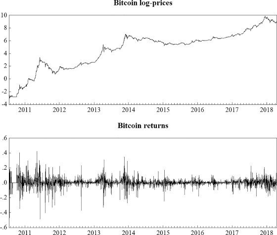
Figure 1: BitCoin price (top panel) and BitCoin returns (bottom panel)

References

- [1] Aalborg, H.A., P. Molnár and J.E. de Vries (2018) What can explain the price, volatility and trading volume of BitCoin? Finance Research Letters Forthcoming.
- [2] Barber, S., X. Boyen, E. Shi, and E. Uzun (2012). Bitter to Better-How to Make BitCoin a Better Currency. In Financial Cryptography and Data Security. Vol. 7397, of Lecture Notes in Computer Science, edited by, Keromytis, A. D., 399-414. Berlin: Springer.
- [3] Baur, D.G., K. Hong and A.D. Lee (2018). BitCoin: Medium of exchange or speculative assets? Journal of International Financial Markets, Institutions and Money 54: 177-189.
- [4] Bollerslev, T. (1986). Generalized autoregressive conditional heteroskedasticity. Journal of Econometrics 31: 307-27.
- [5] Bouoiyour, J., and R. Selmi (2015). What Does BitCoin Look Like? MPRA Paper No. 58091. Germany: University Library of Munich.
- [6] Bouoiyour, J., R. Selmi, A.K. Tiwari, O.R. Olayeni (2016). What drives BitCoin price? Economics Bulletin, 36(2): 1-9.
- [7] Bouri, E., P. Molnár, G. Azzi, D. Roubaud and L.I. Hagfor (2017). On the hedge and safe haven properties of BitCoin: Is it really more than a diversifier? Finance Research Letters 20: 192-198.
- [8] Brooks, Ch. (2014). Introductory econometrics for finance. Cambridge university press.
- [9] Brownlees, C.T., Engle, R.F., Kelly, B.T. (2011). A practical guide to volatility forecasting through calm and storm (August 1, 2011). http://dx.doi.org/10.2139/ssrn.1502915
- [10] Buchholz, M., J. Delaney, J. Warren, and J. Parker (2012). Bits and Bets, Information, Price Volatility, and Demand for BitCoin, Economics 312. www.bitcointrading.com/pdf/bitsandbets.pdf.
- [11] Cermak, V. (2017). Can BitCoin become a viable alternative to fiat currencies? An empirical analysis of BitCoin’s volatility based on a GARCH model. https://ssrn.com/abstract=2961405
- [12] Chen, S. et al., (2016). A first econometric analysis of the CRIX family. https://ssrn.com/abstract=2832099
- [13] Chu,J., Chan, S., Nadarajah, S. and J. Osterrieder. (2017). GARCH Modelling of Cryptocurrencies, Journal of Risk and Financial Management, 10(4), 1-15.
- [14] Ciaian, P., M. Rajcaniova, D. Kancs (2016). The economics of BitCoin price formation. Applied Economics, 48 (19), 1799-1815.
- [15] Ciaian, P., M. Rajcaniova, D. Kancs (2018). Virtual relationships: Short- and long-run evidence from BitCoin and altcoin markets. Journal of International Financial Markets 52: 173-195.
- [16] Dyhrberg, A.H. (2016a). Hedging capabilities of BitCoin. Is it the virtual gold? Finance Research Letters 16: 139-44.
- [17] Dyhrberg, A.H. (2016b). BitCoin, gold and the dollar–A GARCH volatility analysis. Finance Research Letters 16: 85-92.
- [18] Dwyer, P. Gerald 2015, The economics of BitCoin and similar private digital currencies, Journal of Financial Stability, 17, 81-91.
- [19] Engle, R.F. (1982) Autoregressive conditional heteroscedasticity with estimates of the variance of United Kingdom inflation. Econometrica, 987-1007.
- [20] Fisher I. (1911), The Purchasing Power of Money.
- [21] Folkinshteyn D, Lennon M, Reilly T (2015) The BitCoin mirage: an oasis of financial remittance. Journal of International Studies, 10:118-124.
- [22] Gandal, N., J.T. Hamrick, T. Moore, T. Oberman (2018). Price manipulation in the BitCoin ecosystem. Journal of Monetary Economics 95: 86-96.
- [23] Grinberg, R. (2011). BitCoin: An Innovative Alternative Digital Currency. Hastings Science and Technology Law Journal 4: 159-208.
- [24] Gronwald, M. (2014). The economics of bitcoins market characteristics and price jumps. (December 29, 2014). CESifo Working Paper Series No. 5121. https://ssrn.com/abstract=2548999
- [25] Hansen, P.R., Lunde, A. (2005). A forecast comparison of volatility models: does anything beat a garch (1, 1)? Journal of applied econometrics, 20, 873-889.
- [26] Howden, D. (2013). The Quantity Theory of Money. Journal of Prices and Markets 1.1: 17-30.
- [27] Jang, H. and Lee J. (2018). An Empirical Study on Modeling and Prediction of BitCoin Prices With Bayesian Neural Networks Based on Blockchain Information. IEEE Access 6: 5427-5437.
- [28] Kalev, P., Liu, W., Pham, P. K. and E. Jarnecic (2004). Public Information Arrival and Volatility of Intraday Stock Returns. Journal of Banking and Finance, 28, 1441-1467
- [29] Katsiampa, P. (2017). Volatility estimation for BitCoin: A comparison of GARCH models. Economics Letters. 158: 3-6.
- [30] Keynes, J.M., 1936. The General Theory of Employment, Interest and Money. Macmillan, London.
- [31] Kristoufek, L. (2013). BitCoin Meets Google Trends and Wikipedia: Quantifying the Relationship between Phenomena of the Internet Era. Scientific Reports 3 (3415): 1-7.
- [32] Letra, I.J.S. (2016). What drives cryptocurrency value? A volatility and predictability analysis. https://www.repository.utl.pt/handle/10400.5/12556
- [33] Mankiw N.G. (2007) Macroeconomics, 6th edn. Worth Publishers, New York.
- [34] Moore, T., and N. Christin. 2013. Beware the Middleman: Empirical Analysis of BitCoin-Exchange Risk. Financial Cryptography and Data Security 7859: 25-33.
- [35] Poon, S.H., Granger, C. (2005). Practical issues in forecasting volatility. Financial Analysts Journal, 61, 45-56.
- [36] Stavroyiannis, S. and V. Babalos. (2017). Dynamic properties of the BitCoin and the US market. https://ssrn.com/abstract=2966998
- [37] Urquhart, A. (2017). The volatility of BitCoin. https://ssrn.com/abstract=2921082
- [38] van Wijk, D. (2013). What can be expected from the BitCoin? Working Paper No. 345986. Rotterdam: Erasmus Rotterdam Universiteit.
- [39] Vlastakis, N. and R.N. Markellos. (2012). Information demand and stock market volatility. Journal of Banking and Finance, 36, 1808-1821.