Thermal optimization of Curzon-Ahlborn heat engines operating under some generalized efficient power regimes

Abstract

In order to establish better performance compromises between the process functionals of a heat engine, in the context of finite–time thermodynamics (FTT), we propose some generalizations for the well known Efficient Power function through certain variables called ”Generalization Parameters”. These generalization proposals show advantages in the characterization of operation modes for an endoreversible heat engine model. In particular, with introduce the $k$–Efficient Power regime. For this obejctive function we find the performance of the operation of some power plants through the parameter $k$. Likewise, for plants that operate in a low efficiency zone, within a configuration space, the $k$ parameter allow us to generate conditions for these plants to operate inside of a high efficiency and low dissipation zone.

05.70-Ln Nonequilibrium and irreversible thermodynamics; 84.60.Bk Performance characteristics of energy conversion system; figure of merit 89.30.-g Fossils fuels and nuclear power.

1 Introduction

One of the main objectives in the study of thermal engines is to improve their energy performance. Some efforts have focused on reducing the effects associated with the dissipation of energy during the operation of thermal engines [1, 2, 3], other ones have directed to design new energy converters that use higher energetic density fuels [4, 5, 6]. One example of the above is the development of different types of power plants, whose purpose has been to increase the efficiency of energy conversion. The result of this effort has led to the construction of combined cycle plants, which have exhibited a good improvement in their efficiencies, but their energy dissipation in form of heath to the atmosphere continues to be wasted in large quantities. Nevertheless, it is not yet achieved to a large extent establish a compromise between the way of operating an energy converter and a modification in its engineering, without having to build a whole new machine [7, 8, 9]. To establish this trade off, we use a FTT description which has emulated the performance of an energy converter by using diverse objective functions [10, 11, 12, 13, 14, 15, 16]. This new way of studying thermal machines led Curzon and Ahlborn to propose in 1975 [17] one of the first models that presents the power output as an objective function. This function distinguishes the maximum power output as a well–known mode of operation for heat engines. Ever since, several authors have proposed other objective functions, which are not only formed with the individual process functionals (power output, efficiency and dissipation), but also present a good compromise between them [18, 19, 21]. All above with the aim of characterizing optimal operating regimes. However, despite the current approaches that are describing some of the energy converters in good performance regimes, no systematic method has been found with which those type of objective functions can be built. In recent papers, it has been possible to find and quantify the best compromise between the process variables involved through certain criteria of merit, and they have given rise to some proposals for their generalization. In particular, these happened for the ecological ($E=P-\Phi$, being $P$ the power output and $\Phi$ the dissipation function) [18, 19, 20] and omega $(\Omega=E_{u,e}-E_{u,p})$ functions [21, 22, 23]. These new generalized functions contain the so-called generalization parameters, for example for the case of generalized ecological function $E=P-\epsilon\Phi$ the generalized paremeter is $\epsilon$ and for the generalized omega function $\Omega=E_{u,e}-\lambda E_{u,p}$ is $\lambda$. Which in rule allows out obtaining a large family of objective functions [23]. In the endoreversible, the non-endoreversible and irreversible models, the generalized ecological and omega functions have the same maxima [7, 9, 22, 23, 24].

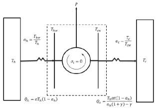
Figure 1: The well-known diagram of a Curzon–Ahlborn (CA) heat engine.

Another proposal of commitment function was defined by Stucki [25] within the context of the Linear Nonequilibrium Thermodynamics called ”economic power output”, which describes with certain approximation, the oxidative phosphorylation process that is involved in the synthesis of adenosine triphosphate inside mitochondrias. After that, Yilmaz [26] in an independent way proposed the same Stucki’s objective function but in the frame of the FTT. His intention was to get a trade-off between the delivered power and the efficiency for a heat engine. He called this new function: ”Efficient Power”, defined as the product of the power output by the efficiency:

$$P_{\eta}=P\eta.$$ (1)

The general idea of all above mentioned works, in which are found functions that accomplish good performance regimes for energy conversion processes, is that the modes of operation are physically attainable. It leads us to the freedom to propose new objective functions at best or set up other generalizations for the functions already known, taking care of the limits of its physical validity. Although the study carried out in this work is effected for an endoreversible model and with linear heat transfer laws, this model is able to set operating ranges for more real models, focusing attention on the mechanisms of heat exchange that in heat engines could be modified to what we have called ”restructuring conditions”.

As we have pointed out, we are representing the irreversibilities between the working substance and the external energy reservoirs through a Newtonian heat transfer law. Therefore, we can write the input $\left(Q_{h}\right)$ and output $\left(Q_{c}\right)$ heat fluxes as:

$$Q_{h}=\alpha\left(T_{h}-T_{hw}\right),$$ (2)

$$Q_{c}=\beta\left(T_{cw}-T_{c}\right),$$ (3)

where $\alpha$ and $\beta$ are the thermal conductances, whereas that $T_{hw}$ and $T_{cw}$ are the temperatures of the working substance. In addition, as in the Curzon–Ahlborn (CA) model, the responsible processes in the production of work can be identified, as the interchange of energy between the working substance and the reservoirs (see Fig. 1). The total entropy production of the heat engine is:

$$\sigma_{T}=\sigma_{e}+\sigma_{ws}\geq 0,$$ (4)

with $\sigma_{e}$ is the entropy production at the coupling between the working substance and the surroundings and $\sigma_{ws}$ is the working substance entropy production. In particular, for the model shown in Fig. 1, $\sigma_{e}$ is given as:

$$\sigma_{e}=\frac{Q_{c}}{T_{c}}-\frac{Q_{h}}{T_{h}},$$ (5)

while $\sigma_{ws}$ is:

$$\sigma_{ws}=\frac{Q_{h}}{T_{hw}}-\frac{Q_{c}}{T_{cw}}+\sigma_{i},$$ (6)

being $\sigma_{i}$ the internal entropy production which is attributed to different causes, such as turbulence, viscosity, among others. The working substance operates in cycles, then $\sigma_{ws}=0$ and for the endoreversible model, we have $\sigma_{i}=0$, so the Eq. 6 can be rewritten as follows,

$$\frac{Q_{h}}{T_{hw}}=\frac{Q_{c}}{T_{cw}}.$$ (7)

Eq. 7 represents the well-known endoreversibility hypothesis (Citar Rubin). While the surroundings entropy production continues to fulfill that,

$$\frac{Q_{c}}{T_{c}}-\frac{Q_{h}}{T_{h}}>0.$$ (8)

In the following, we express the heat fluxes $Q_{h}$ and $Q_{c}$ in terms of an auxiliary variable called high reduced temperature $\left(a_{h}=T_{h}/T_{hw}\right)$, thus:

$$Q_{h}\left[\alpha,T_{h},a_{h}\right]=\alpha T_{h}\left(1-a_{h}\right)$$ (9)

and

$$Q_{c}\left[\alpha,\gamma,T_{h},\tau,a_{h}\right]=\frac{\alpha T_{h}\tau\left(1-a_{h}\right)}{a_{h}-\gamma\left(1-a_{h}\right)},$$ (10)

where $\gamma=\alpha/\beta$ and $\tau=T_{c}/T_{h}$. Besides, $Q_{c}$ can be expressed in terms of $a_{h}$ by Eq. 7 which shows the internal irreversibilities occurring in the energy conversion process. In principle, the heat fluxes $Q_{h}$ and $Q_{c}$ can characterize the behavior of this CA heat engine. Although, the aforementioned process variables become the objective functions of our interest.

The process variables represent the energetic behavior of an engine, and under the considerations we have made in the paragraph after Eq. (6) for the heat fluxes $Q_{h}$ and $Q_{c}$, we have the following characteristic functions:

$$P[\alpha,\gamma,T_{h},\tau,a_{h}] = Q_{h}-Q_{c}$$ (11)

$$= \frac{\alpha T_{h}\left(1-a_{h}\right)\left[a_{h}-\gamma\left(1-a_{h}\right)-\tau\right]}{a_{h}-\gamma\left(1-a_{h}\right)},$$

$$\eta\left[\gamma,\tau,a_{h}\right] = 1-\frac{Q_{c}}{Q_{h}}$$ (12)

$$= 1-\frac{\tau}{a_{h}-\gamma\left(1-a_{h}\right)}$$

and

$$\Phi\left[\alpha,\gamma,T_{h},\tau,a_{h}\right]=T_{c}\sigma_{T} = Q_{c}-\tau Q_{h}$$ (13)

$$= \frac{\alpha T_{h}\tau\left(1+\gamma\right)\left(1-a_{h}\right)^{2}}{a_{h}-\gamma\left(1-a_{h}\right)}$$

In principle, these functions contain all the thermodynamic information of the system, they are normally used to limit the operating ranges of the real thermal machines.

This article is organized as follows, in Sect. 2, we introduce three generalization proposals for the Efficient Power $\left(P_{\eta}\right)$, and we make an energetic analysis of each of them. In Sect. 3, we characterize the behavior of some power plants by using the proposal of the $k$–Efficient Power, since this generalized function identifies all the physically accessible points of the Power Output vs. Efficiency curve. Also, we show how the generalization parameters allow us to modify aspects of the operation of a heat engine. Finally, in Sect. 4 we enunciate the concluding remarks of this work.

2 Generalizations of the Efficient Power

One of the problems in the study of energy conversion for any heat engine, is characterize all the operation modes to which a thermal machine can gain access [23], this problem lies in the lack of objective functions associated to those modes. In this work, we propose a generalization of the objective function “Efficient Power”, in order to describe the largest number of accessible operation modes for a heat engine [27]. This generalized function can be written as,

$$P\eta_{g}=\left(P^{\sigma}\eta^{\upsilon}\right)^{\chi}.$$ (14)

However, this generalization is reduced to three particular cases, which only lead to define a single generalization parameter, because in [23] it has been shown that a single parameter is enough to associate the particular performance of a thermal engine with a specific mode of operation. In each of them, different modes of operation can be achieved for the CA energy converter model.

When $\chi$ parameter is $\chi=\nicefrac{{1}}{{\sigma}}$, we can define the exponent that acts in efficiency as $k=\nicefrac{{\upsilon}}{{\sigma}}$ and we get the commitment function named as $k$–Efficient Power [23]. Given by:

$$P\eta_{k}=P\eta^{k}.$$ (15)

If $\chi=\nicefrac{{1}}{{\upsilon}}$, we can determine the exponent on the power output as $l=\nicefrac{{\sigma}}{{\upsilon}}$. We call this function $l$–Efficient Power, whose expression is,

$$P\eta_{l}=P^{l}\eta.$$ (16)

Finally, in case $\upsilon=\sigma=1$, we have the function $\chi$-Efficient Power, defined by

$$P\eta_{\chi}=\left(P\eta\right)^{\chi}.$$ (17)

Upon this, we will analyze some of the characteristics that each of the different generalization proposals has got.

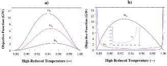
Figure 2: Graph of generalized commitment functions: $k$–Efficient Power, $l$–Efficient Power and $\chi$–Efficient Power. By using the values, $\alpha=1\left[\textrm{MW}/\textrm{K}\right],\ \gamma=3,\ T_{h}=500\left[\textrm{K}\right]$, with a) $\ k=\ l=\chi=1.5$ and b) $\ k=\ -0.01,l=\ -2,\chi=-0.5$. Note in a) all the maximums are in different places, in spite of the generalization parameters are equal, they do not correspond at the same value of $a_{h}$. In b) all the parameters have different values because the domain of these functions is not the same.

2.1 Energetics under the $k$–Efficient Power operation mode

By substituting the Eqs. 11 and 12 in the Eq. 15, we get the explicit expression for the $k$–Efficient Power,

$$P\eta_{k}=T_{h}\alpha\left[1-a_{h}\right]\left[1-\frac{\tau}{a_{h}-\left(1-a_{h}\right)\gamma}\right]^{1+k}.$$ (18)

Where $-1\leq k$, so that Eq. 18 has physical validity [23]. From the Fig. 2a, it is possible to remark there exists an $a_{h}$ that maximizes the $k$–Efficient Power, which is:

$$a_{h}^{mP\eta_{k}}\left[\gamma,\tau,k\right]=\frac{2\gamma-k\tau+\sqrt{\tau\left(4+4k+k^{2}\tau\right)}}{2\left(1+\gamma\right)}.$$ (19)

The process variables evaluated in this regime are:

$$P\left(\alpha,\gamma,\tau,T_{h},k\right)=T_{h}\alpha\frac{\left[\left(2+k\right)\sqrt{\tau}-\sqrt{4+k\left(4+k\tau\right)}\right]\left[2+k\tau-\sqrt{\tau}\sqrt{4+k\left(4+k\tau\right)}\right]}{2\left(1+\gamma\right)\left[k\sqrt{\tau}-\sqrt{4+k\left(4+k\tau\right)}\right]},$$ (20)

$$\eta\left(\tau,k\right)=\frac{2+k\left(2-\tau\right)-\sqrt{\tau}\sqrt{4+k\left(4+k\tau\right)}}{2\left(1+\gamma\right)},$$ (21)

and

$$\Phi\left(\alpha,\gamma,\tau,T_{h},k\right)=T_{h}\alpha\frac{\sqrt{\tau}\left[2+k\tau-\sqrt{\tau}\sqrt{4+k\left(4+k\tau\right)}\right]^{2}}{2\left(1+\gamma\right)\left[\sqrt{4+k\left(4+k\tau\right)}-k\sqrt{\tau}\right]}.$$ (22)

From the Eq. 19, we note that this high reduced temperature not only maximizes the $k$–Efficient Power, but it depends on the generalization parameter. In Fig. 3 it can be shown how the process variables are affected by the generalization parameter $k$. However, the greater effect is reflected in the dissipation, since increasing the value of $k$, it decreases faster than the power output. On the other hand, the effect of this parameter makes the efficiency reach a constant value, that is, the heat engines that operate at maximum $k$–Efficient Power tend to the maximum efficiency regime and therefore, the operation modes close to it are difficult to achieve. We can also find the following limits for the process variables in the maximum $k$–Efficient Power regime,

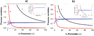
Figure 3: Energetics in the regime of maximum $k$–Efficient Power, in which we have used values of: $\gamma=3,\ T_{h}=500\textrm{K},\ \alpha=1\left[\textrm{MW}/\textrm{K}\right].$ In Figure (a) we took $\tau=0.5$ and for (b) $\tau=0.8$. Where $\eta$ is the efficiency, $P$ is the power output in $\left[\textrm{GW}\right]$, $\Phi$ is the dissipation in $\left[\textrm{GW}\right]$ and $\eta_{C}$ the Carnot efficiency as the reversible limit.

$$\lim_{k\rightarrow\infty}P = 0,$$

$$\lim_{k\rightarrow\infty}\eta = 1-\tau,$$ (23)

$$\lim_{k\rightarrow\infty}\Phi = 0.$$

2.2 Energetics under the $l$–Efficient Power operation mode

The $l$–Efficient Power can be written as:

$$P\eta_{l}=\left[T_{h}\alpha\left(1-a_{h}\right)\right]^{l}\left[1-\frac{\tau}{a_{h}+\gamma\left(a_{h}-1\right)}\right]^{l+1},$$ (24)

where $l\in\left(-\infty,-1\right]\cup\left(0,\infty\right)$ otherwise it would not exhibit attainable physical properties. In the same way, this commitment function has two different high reduced temperatures that maximize it (Fig. 4), the first one:

$$a_{h1}^{mP\eta_{l}}\left[\gamma,\tau,l\right]=\frac{2l\gamma-\tau+\sqrt{\tau\left[4l\left(1+l\right)+\tau\right]}}{2l\left(1+\gamma\right)},$$ (25)

represents a maximum located in the zone where the energy converter operates as a heat engine for $l\in\left(0,\infty\right)$. Beneath these same conditions, the second high reduced temperature

$$a_{h2}^{mP\eta_{l}}\left[\gamma,\tau,l\right]=\frac{2l\gamma-\tau-\sqrt{\tau\left[4l\left(1+l\right)+\tau\right]}}{2l\left(1+\gamma\right)}$$ (26)

depicts a minimum (see Fig. 2b), which is in the region where the energy converter does not operates as a heat engine. With this operation regimen, the process variables become,

$$P_{1}\left(\alpha,\gamma,\tau,T_{h},l\right)=T_{h}\alpha\frac{\left[\left(1+2l\right)\sqrt{\tau}+\sqrt{4l\left(1+l\right)+\tau}\right]\left[2l+\tau+\sqrt{\tau}\sqrt{4l\left(1+l\right)+\tau}\right]}{2l\left(1+\gamma\right)\left[\sqrt{\tau}+\sqrt{4l\left(1+l\right)+\tau}\right]},$$

$$\eta_{1}\left(\tau,l\right)=\frac{2\left(1+l\right)-\tau+\sqrt{\tau}\sqrt{4l\left(1+l\right)+\tau}}{2\left(1+l\right)}$$

and

$$\Phi_{1}\left(\alpha,\gamma,\tau,T_{h},l\right)=-T_{h}\alpha\frac{\sqrt{\tau}\left[2l+\tau+\sqrt{\tau}\sqrt{4l\left(1+l\right)+\tau}\right]^{2}}{2l\left(1+\gamma\right)\left[\sqrt{\tau}+\sqrt{4l\left(1+l\right)+\tau}\right]}.$$

While

$$P_{2}\left(\alpha,\gamma,\tau,T_{h},l\right)=T_{h}\alpha\frac{\left[\left(1+2l\right)\sqrt{\tau}-\sqrt{4l\left(1+l\right)+\tau}\right]\left[2l+\tau-\sqrt{\tau}\sqrt{4l\left(1+l\right)+\tau}\right]}{2l\left(1+\gamma\right)\left[\sqrt{\tau}-\sqrt{4l\left(1+l\right)+\tau}\right]},$$

$$\eta_{2}\left(\tau,l\right)=\frac{2\left(1+l\right)-\tau-\sqrt{\tau}\sqrt{4l\left(1+l\right)+\tau}}{2\left(1+l\right)}$$

and

$$\Phi_{2}\left(\alpha,\gamma,\tau,T_{h},l\right)=T_{h}\alpha\frac{\sqrt{\tau}\left[2l+\tau-\sqrt{\tau}\sqrt{4l\left(1+l\right)+\tau}\right]^{2}}{2l\left(1+\gamma\right)\left[\sqrt{4l\left(1+l\right)+\tau}-\sqrt{\tau}\right]}.$$

When $l\in\left(-\infty,-1\right]$, the Eq. 25, still represents a maximum, though. It is located in the zone where the thermal machine does not work as a heat engine. Analogously, it happens with the Eq. 26.

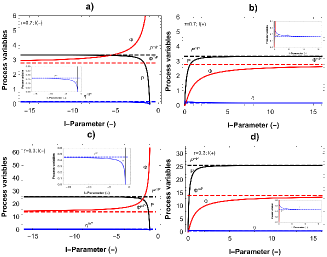
Figure 4: Energetics at the regime of maximum $l$–Efficient Power for two values of $\tau$, in which we have used values of: $\gamma=3,\ T_{h}=500\textrm{K},\ \alpha=1\left[\textrm{MW}/\textrm{K}\right]$. In graphs a, b, c and d we show the effect of $a_{h1}$ and $a_{h2}$. With $P$ the power output in $\left[\textrm{GW}\right]$, $\Phi$ the dissipation in $\left[\textrm{GW}\right]$, $\eta$ the efficiency and the superscript $mP$ indicates the energetic of the system evaluated in the maximum power regime as the limit for each function.

In Fig. 4 we can see two regions in which the process variables operationally describe the energy converter as a heat engine. These regions are separated by the point that characterizes the maximum power output regime. The behavior of process variables tend to very specific limits, given by:

$$\lim_{l\rightarrow\pm\infty}P = T_{h}\alpha\frac{\left(\sqrt{\tau}-1\right)^{2}}{1+\gamma}$$

$$\lim_{l\rightarrow\pm\infty}\eta =1- \sqrt{\tau}$$ (27)

$$\lim_{l\rightarrow\pm\infty}\Phi = T_{h}\alpha\frac{\sqrt{\tau}\left(\sqrt{\tau}-1\right)^{2}}{1+\gamma}.$$

This function has a clear disadvantage with respect to the $k$–Efficient Power, if you want to study the real energy converters (heat engines), because this function does not include a point which is physically accessible: the maximum power output regime.

2.3 Energetics under the $\chi$-Efficient Power operation mode

In the case of $\chi$–Efficient Power. The model of the function has the following shape,

$$P\eta_{\chi}=\left[\frac{T_{h}\alpha\left(1-a_{h}\right)\left\{\gamma+\tau-a_{h}\left(1+\gamma\right)\right\}^{2}}{\left(a_{h}+\gamma\left(a_{h}-1\right)\right)^{2}}\right]^{\chi}.$$ (28)

This function also presents an extreme value at the high reduced temperature and that maximizes it (see Fig. 2a). This value is:

$$a_{h}^{mP\eta_{\chi}}[\gamma,\tau]=\frac{2\gamma-\tau+\sqrt{\tau\left(8+\tau\right)}}{2\left(1+\gamma\right)},$$ (29)

As can be beheld, in Eq. 29, this high reduced temperature that characterizes the optimal regime for this generalization, does not depend on the parameter $\chi$. It coincides with the same results that has already been obtained for Efficient Power [26].

2.4 A comparison between the different generalization proposals

The initial analysis presented below has the objective of comparing the mathematical forms of the generalization proposals, whose generalization parameter appears explicitly in the energetics of every heat engine, in order to show some advantages of each one of their operation modes.

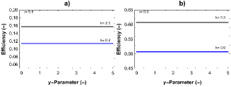
Figure 5: Comparison between the efficiencies at maximum $k$–Efficient Power for four different values of $k$ and two values of $\tau$.

It is possible to detect certain differences in relation to the optimal regimes that each one of them let us to reach. In Fig. 5 the efficiencies are completely different for the values that can be assumed by $l$ and $k$ respectively.

In general, the generalization parameters play a big role in the optimization processes for energy converters. For instance, from the graphs of Fig. 5 we can observe the behavior of efficiency for two different values of $\tau$. In particular, the graphs a) and b) of Fig. 5 make evident the experimental fact that occurs in the mesoscopic energy converters, which operate within very small temperature gradients $(T_{c}\thickapprox T_{h})$ and therefore, their efficiencies are low [28, 29, 30]. This is because the system become saturated and the energy conversion processes stop. In contrast with macroscopic systems, where the restriction in the temperature relationship does not exist, since the energy reservoirs are considered large enough as for the thermal machines to operate continuously and achieve greater efficiencies. Another consequence of implementing the parameters of generalization in objective functions is the possibility of improving efficiency and in general any of the process variables, i.e., they enable to modify the heat engine performance.

3 Effects on the construction and improvements in some power plants

The operation of a thermal machine takes into account a significant number of variables, since most of them are related not only to the design of the energy converter but also to the mode of operation that can be achieved. From the CA model we denote the parameter $\gamma$ as the relationship exists between the thermal conductances, which modulate the energy exchange with the reservoirs. While the relationship between the temperatures of the reservoirs $\tau$ is related to the operating range of this converter, i.e., it bounds the capacity of the system to convert energy. Due to the above, we will consider these two parameters as control elements in the performance of a heat engine, they modulate the amount of energy that gets in and gets out the system. On the other hand, as we have already pointed out the parameter $k$ allows to describe the gains or losses of energy which are reflected in the process variables of a heat engine.

In [23] has been shown the generalization parameter $k$ can help us to reach any operation mode that allows an energy converter to work as a heat engine. This has certain advantages, because the $k$ generalization parameter indicates whether the thermal machine operates in a low efficiency (LE) and high dissipation (HD) zone or in one of high efficiency (HE) and low dissipation (LD). We consider those operation modes whose efficiency values are bounded between the efficiency in the maximum power regime and Carnot regime, this operation modes belong to HE zone and therefore their dissipation values are in the LD zone.

If we have any of the process variables (Eqs. 11, 12 and 13), we can establish, through the $k$–Efficient Power regime, the relations that exist between the parameter $k$ and the energetic of the heat engine, given by:

$$k_{LE}\left(\alpha,\gamma,T_{h},\tau,P\right) = \frac{P^{2}\left(\gamma+1\right)^{2}+T_{h}\alpha\left(1-\tau\right)\left[T_{h}\alpha\left(1-\tau\right)-\varLambda\right]-P\left(1+\gamma\right)\left[2T_{h}\alpha\left(1+\tau\right)+\varLambda\right]}{2PT_{h}\alpha\tau\left(1+\gamma\right)}$$ (30)

$$k_{HE}\left(\alpha,\gamma,T_{h},\tau,P\right) = \frac{P^{2}\left(\gamma+1\right)^{2}+T_{h}\alpha\left(1-\tau\right)\left[T_{h}\alpha\left(1-\tau\right)+\varLambda\right]-P\left(1+\gamma\right)\left[2T_{h}\alpha\left(1+\tau\right)+\varLambda\right]}{2PT_{h}\alpha\tau\left(1+\gamma\right)}$$ (31)

$$k\left(\tau,\eta\right) = \frac{1-\tau-\eta\left(2-\eta\right)}{\left(1-\eta\right)\left(\eta+\tau-1\right)}$$ (32)

$$k_{HE}\left(\alpha,\gamma,T_{h},\tau,\Phi\right) = \frac{\left(1+\gamma\right)\Phi\left[\Xi-\left(1+\gamma\right)\sqrt{\Phi}\right]+T_{h}\alpha\tau\left[\left(1-\tau\right)\Xi-\left(1+\gamma\right)\left(3+\tau\right)\sqrt{\Phi}\right]}{2T_{h}\alpha\left(1+\gamma\right)\sqrt{\Phi}\tau^{2}}$$ (33)

$$k_{LE}\left(\alpha,\gamma,T_{h},\tau,\Phi\right) = -\frac{\left(1+\gamma\right)\Phi\left[\Xi+\left(1+\gamma\right)\sqrt{\Phi}\right]+T_{h}\alpha\tau\left[\left(\tau-1\right)\Xi+\left(1+\gamma\right)\left(3+\tau\right)\sqrt{\Phi}\right]}{2T_{h}\alpha\left(1+\gamma\right)\sqrt{\Phi}\tau^{2}}$$ (34)

where

$$\begin{array}[]{c}\Lambda=\sqrt{P^{2}\left(1+\gamma\right)^{2}+T_{h}^{2}\alpha^{2}\left(1-\tau\right)^{2}-2PT_{h}\alpha\left(1+\gamma\right)\left(1+\tau\right)}\\ \Xi=\sqrt{\left(1+\gamma\right)\left(4T_{h}\alpha\tau+\Phi\left[1+\gamma\right]\right)}\end{array}.$$

The remarkable of the Eqs. 30 and 32 is manifested through an energy analysis applied to a set of 6 power plants (2 of monocycle, 2 of combined cycle and 2 nuclear). In Table 1 the reported manufactured values of: reservoir temperatures ($T_{h}$ and $T_{c}$), efficiency ($\eta$) and operating power output ($P$) for each of them are presented. With this data [31, 32], we use the Eq. 32 to know the value of $k$ that characterizes the operation mode of each power plant, assuming a fixed relationship between the conductances. In addition, with the operating power output and Eq. 30, the value of thermal conductance $\alpha$ is estimated. Finally, from Eq. 19, the high reduced temperature value $(a_{h})$ that characterizes the operation of each plant is reckoned up, with all these parameters, we are able to estimate the dissipated energy of each power plant. In the same Table 1, it is shown a comparison of the values that these plants should have if they operate in any of the already well-known regimes (maximum power output $\left(MP\right)$, maximum efficiency $\left(M\eta\right)$, maximum ecological function $\left(ME\right)$, maximum efficient power $\left(MP_{\eta}\right)$ and maximum generalized ecological function $\left(ME_{g}\right)$).

Table 1: Operation data for different commercial power plants [31, 32]. A comparison of these reported power output ($P_{r}$) and efficiency ($\eta_{r}$) against the values of these process variables would reach for different operation modes already known: $MP$, $M\eta$, $MP\eta$, $ME$, y $ME_{g}$. The worth of $k$ that allows to characterize the operation regime of the different power plants, are associated with their corresponding high reduced temperature $(a_{h})$, as well as the dissipation that is generated for their respective operating regime. An arbitrary conductances ratio has been assumed $\left(\gamma=3\right)$ and in each case the value of the conductance $\alpha$ has been calculated which allows to obtain the value of the reported power output.

Power Plant	Almaraz II (A)		Cofrentes (C)		West Thurrock (WT)		Larderello (L)		Toshiba (T)		Alstom (Al)
	(PWR, Spain, 83)		(BWR, Spain, 84)		(Uk, 62)		(Italy,64)		(109FA, 04)		(ka26-1)
Reported Data	$T_{h}[K]$	$T_{c}[K]$	$T_{h}[K]$	$T_{c}[K]$	$T_{h}[K]$	$T_{c}[K]$	$T_{h}[K]$	$T_{c}[K]$	$T_{h}[K]$	$T_{c}[K]$	$T_{h}[K]$	$T_{c}[K]$
	600	290	562	289	838	298	523	353	1573	303	1398	288
	$P_{r}\left[GW\right]$	$\eta_{r}$	$P_{r}\left[GW\right]$	$\eta_{r}$	$P_{r}\left[GW\right]$	$\eta_{r}$	$P_{r}\left[GW\right]$	$\eta_{r}$	$P_{r}\left[GW\right]$	$\eta_{r}$	$P_{r}\left[GW\right]$	$\eta_{r}$
	1.044	0.35	1.092	0.34	1.240	0.36	0.150	0.16	0.342	0.48	0.410	0.57
$P^{MP};\eta^{MP}$	1.0806	0.30	1.1638	0.28	1.2631	0.4	0.1519	0.18	0.3563	0.56	0.4118	0.55
$P^{MP\eta};\eta^{MP\eta}$	0.9944	0.37	1.0683	0.35	1.1759	0.48	0.1378	0.23	0.3379	0.64	0.3899	0.62
$P^{ME};\eta^{ME}$	0.8997	0.40	0.9617	0.38	1.0878	0.51	0.1211	0.25	0.3229	0.66	0.3715	0.65
$P^{ME_{g}};\eta^{ME_{g}}$	0.8127	0.42	0.8749	0.39	0.9525	0.54	0.1140	0.26	0.2709	0.71	0.3128	0.69
$\alpha\left[MW/K\right]$	77.5543		103.5040		36.9997		36.4921		2.8779		3.9509
Generalization Data	$k$		$k$		$k$		$k$		$k$		$k$
	0.5615		0.8174		-0.2966		-0.2211		-0.4569		0.2192
	$a_{h}$		$a_{h}$		$a_{h}$		$a_{h}$		$a_{h}$		$a_{h}$
	0.9359		0.9448		0.8889		0.9509		0.8426		0.8698
$\Phi\left[GW\right]$	0.4971		0.4682		0.9796		0.1547		0.2333		0.1611

From Eqs. 20 and 21, we can use the control parameters to tune the performance of a heat engine. On the other hand, $\tau$ can be associated with a kind of thermal potential, because it accounts for the length of the temperature difference between the external energy reservoirs. As we can note, from Fig. 6 and Table 1, $\tau$ is directly related to the efficiencies that this set of power plants can perform, such is the case of Larderello (L), whose temperature difference between the reservoirs is small, this minimizes the gradient responsible for promoting the energy flux through the converter, i.e., a small number of cycles is generated in the heat engine compared to Cofrentes (C) plant, whose value of $\tau$ is the closest to Larderello one, so that Larderello’s power output is low. Due to the energy conservation, a large amount of heat flux must be transferred to the reservoir at $T_{c}$. From the Eqs. 11, 12 and 13, it is had that for those operation modes whose efficiency is below a half of the Carnot efficiency, the system will dissipate more energy than the power output obtained.

In the case of the conductances ($\alpha$,$\beta$) and their ratio $\left(\gamma\right)$, their greatest effect is reflected in the power output that this kind of converter can deliver as useful energy. According to the CA model, all of power plants express a relationship between the reported power and the value of the parameters ($\gamma$,$\alpha$) (see Table 1). However, when modifying any of these two parameters, the power output can increase or decrease, depending on the value that they acquire (see Fig. 6).

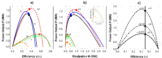
Figure 6: a) Curves of power output vs. efficiency and b) curves of power output vs. dissipation for each of the power plants reported in Table 1. In solid lines the plants that operate in the HE zone are shown [Almaraz II (black, A), Cofrentes (blue, C) and Alston (brown, Al)], while the dashed lines show those ones that work in the LE zone [West Thurrock (red, WT), Toshiba (green, T) and Larderello (orange, L)]. In c) the energetic behavior that Almaraz II achieves for different values of the control parameters $\alpha$ and $\gamma$ is exhibited.

This indicates that the reported values of power output and efficiency of a power plant are not enough information to think of modifying the operation of it. Such is the case of some combined cycle plants, Toshiba 109FA of 2004 (T) it has an efficiency similar to Alston ka26-1 (Al) but with less power output. Although the first one reports a relatively high efficiency compared to the other one, it is operating in the LE and HD zone, while the second one operates in the HE and LD zone (Fig. 6a). In general, this behavior is an evidence of the operating mechanisms to which the power plants are undergone, i.e., the operation of each one defines, from the energy point of view, a family of curves in the configuration space ($\alpha$,$\gamma$, $\tau$, $P$ and $\eta$), it fixes to a well-defined point that represents a characteristic operation regime. From the data for the plants, we can select a specific value of $\tau$, which reduces the number of configurations for each one. It is verified, for example in Almaraz II, that it is possible to assume $\alpha$ or $\gamma$, and then adjust either of the two, so that the reported power output will be reached (Fig. 6b). Although the family of curves that allow us to attain the reported power output is still large, for the assumed parameter ($\gamma$), we are able to obtain only one that adjusts to the value of such power output . Thus, the new configuration is completed and the result is a curve with any accessible operation mode.

In Fig. 6a, it is observed that some power plants already operate in the HE and LD zone. On the contrary, there are some of them which are in the HD and LE zone, and it is possible to find the restructuring conditions that allow them to operate in an optimal configuration, producing the same power output, a gain in efficiency and a decrease in dissipated energy. To accomplish the above, it is important to find the physically achievable efficiency values for a given power output. Then, we calculate $k$ through Eq. 31 and substitute it in the expression for the efficiency (Eq. 21). And it is pointed out that the values of $k>0$ ($k^{\ast}$) are associated with an efficiency located in the HE and LD zone ($\eta^{\ast}$), while the values of $-1<k<0$ leads to an efficiency in the HD and LE zone (see Fig. 7a). On the other hand, $k$ is related with the value of $a_{h}$ that characterizes each operation mode. We noted, if $a_{h}=a_{h}^{\ast}$ is within the HE and LD zone, is longer than the value acquired in the HD and LE zone (Fig. 6). Then, the only way to establish the restructuring condition under the CA model, at the same point in the configuration space, is modifying the reservoir temperature $T_{h}$. This leads us to look for a different configuration from the original one (curve) and that condition guarantees the existence of the reported power output and improved efficiency point, i.e., we assume that $T_{hw}$ remains constant and the relationship must be satisfied,

$$\frac{a_{h}}{a_{h}^{\ast}}=\frac{T_{h}^{\ast}}{T_{h}}.$$ (35)

Note that $T_{h}^{\ast}<T_{h}$. By assuming that the temperature $T_{c}$ keeps unchanged, we can now find a new $\tau=\tau^{RC}$. Analogously, to calculate some data from the Table 1, we take $\tau^{RC}$, the reported power output $P_{r}$ and the efficiency $\eta^{\ast}$ in order to derive new conditions on $\gamma$ and $\alpha$, when we solve the equation system:

$$\eta^{\ast} = \eta\left(\gamma^{RC},\tau^{RC},a_{h}^{\ast}\right),$$

$$P = P\left(\alpha^{RC},\gamma^{RC},\tau^{RC},T_{h}^{\ast},a_{h}^{\ast}\right).$$ (36)

Where the $RC$ index refers to the restructuring condition. The parameters ($\alpha^{RC},\gamma^{RC},\tau^{RC},P$ and $\eta^{\ast}$) represent a new configuration (restructuring configuration) in which the operation mode of each plant is within the HE and LD zone. As can be seen in Table 2, the advantage we find is less dissipation during the operation at the restructuring condition.

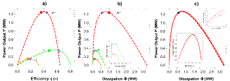
Figure 7: a) Power output vs. efficiency curves for the plants [West Thurrock (red, WT), Toshiba (green, T) and Larderello (orange,L)] whose operating modes are in the LE zone (marked with points), the new operation mode to which each plant can access is also shown, with the same power output but in the HE zone (marked with diamonds). While in b) Power output vs. dissipation curves for the same plants are shown. In c) the power output vs. dissipation and power output vs. efficiency curves are shown for the original WT plant configuration (dashed line), as well as its corresponding curves to the restructuring configuration (solid line). In addition, the original operation point marked with a diamond, the best efficiency under the same configuration and the restructuring condition are highlighted with a star.

Table 2: A comparison between the original operating modes, the same ones with the best efficiency under the original configuration and the new operating regimes within the restructuring condition for the WT, L and T power plants.

Plant	$k\notin HE$	$k\in HE$	$T_{h}/T_{h}^{\ast}$	RC		$PV\notin HE$		$PV\in HE$		$PV^{RC}$
West Thurrock (WT)	-0.2966	0.4217	0.9768	$\alpha^{RC}\left[MW/K\right]$	37.8776	$P\left[GW\right]$	1.24	$P\left[GW\right]$	1.24	$P\left[GW\right]$	1.24
				${}^{\gamma^{RC}}$	2.8313	$\eta$	0.36	$\eta^{\ast}$	0.44	$\eta$	0.44
				$\tau^{RC}$	0.3640	$\Phi\left[GW\right]$	0.98	$\Phi^{\ast}\left[GW\right]$	0.558	$\Phi\left[GW\right]$	0.535
Larderello (L)	-0.2211	0.2838	0.9905	$\alpha^{RC}\left[MW/K\right]$	36.8422	$P\left[GW\right]$	0.15	$P\left[GW\right]$	0.15	$P\left[GW\right]$	0.15
				${}^{\gamma^{RC}}$	2.7986	$\eta$	0.16	$\eta^{\ast}$	0.20	$\eta$	0.20
				$\tau^{RC}$	0.6814	$\Phi\left[GW\right]$	0.15	$\Phi^{\ast}\left[GW\right]$	0.098	$\Phi\left[GW\right]$	0.093
Toshiba (T)	-0.4569	0.8412	0.9575	$\alpha^{RC}\left[MW/K\right]$	3.0056	$P\left[GW\right]$	0.342	$P\left[GW\right]$	0.342	$P\left[GW\right]$	0.342
				${}^{\gamma^{RC}}$	2.8077	$\eta$	0.48	$\eta^{\ast}$	0.630	$\eta$	0.63
				$\tau^{RC}$	0.2012	$\Phi\left[GW\right]$	0.23	$\Phi^{\ast}\left[GW\right]$	0.097	$\Phi\left[GW\right]$	0.092

The curves that can be generated from a point in the configuration space and represent an operating regime for a thermal machine, contain also other operating regimes that are achievable, as long as there are physically acceptable relationships for the control parameters.

4 Conclusions

Although, the way thermal machines exchange heat with the surroundings depends strongly on the type of the proposed heat transfer law, their energy optimization goes beyond the irreversibilities that can be introduced in the model. The type of irreversibilities the CA model does not take into account are the internal ones of the system (working substance), that in practice are difficult to quantify. Nevertheless, the CA model provides boundary operating conditions that take into account both the energy (power output, efficiency and dissipation) and the parameters related to the construction of the energy converter (thermal conductance and temperatures quotient). On the other hand, the CA model allows to establish the concept of objective function, a relationship between the process variables that exhibits an optimal behavior.

Within the generalization proposals for the efficient power as an objective function, the $k$–Efficient Power presents a clear advantage, it can characterize modes of operation that are not achievable for the other proposals. As the high reduced temperature ($a_{h}$) that characterizes the maximum $k$–Efficient Power regime can be written in terms of the generalization parameter $k$, a biunivocal relationship between both variables is established. This means, it is possible to associate any process variable with this generalization parameter and study all the physically accessible operating regimes at the same time.

The conversion efficiency usually is found among the reported data of power plants. For this reason, it is a candidate that permits to find the value of $k$, since this function requires a minimum amount of system information [$k(\eta,\tau)$]. This dimensionless parameter allows us to say, in the particular case of power plants, if their operation modes are within the HE zone or outside it. While in the case of power or dissipation, we require more information from the system to locate the operation modes in the configuration space (HE or LE). This extra information must be estimated, because the control parameters $\alpha$ and $\gamma$ modulate the amount of useful work obtained.

With the $k$–Efficient Power model that we have been analyzing, we found the most suitable configurations for $\alpha,\gamma$, $\tau$, $P$ and $\eta$ that fit the operation of some power plants. Likewise, we show the parameter $k$ is capable of building any energy curve ($P$ vs. $\eta$ and $P$ vs. $\Phi$) compatible with some attainable regime. If we move the characteristic operating point for each power plant in this set of configurations on a curve with an optimal energetic performance, we can establish the “restructuring conditions” on the control parameters for all plants that are operating in the LE zone. The advantage of this new configuration is that the plant will operate in the HE zone, decreasing its dissipation without sacrificing power output. Such is the case of the monocycle plants (see Fig. 7), those plants are operating outside the HE zone and also the Toshiba 109FA, which is a combined cycle. All of the above is summarized in the following: the operating regimes, which come from an objective function and that are also associated to a generalization parameter determine in the space of energy configurations, families of curves linked to the values of the control parameters (design). If the values of these parameters are modified, the optimal performance of an energy converter is guaranteed without having to build a new one.

References

- [1] M. A. Barranco–Jimenez, F. Angulo–Brown, J. Appl. Phys. 80, 4872 (1996).
- [2] P. L. Curto–Risso, et al., Appl. Energy 88, 1557 (2011).
- [3] S. Sánchez–Orgaz, A. Medina, A. Calvo Hernández, Energy Convers. Manag. 67, 171 (2013).
- [4] A. De Vos, Energy, Convers. Manag. 36, 1 (1995).
- [5] T. Miyazaki, et al., Energy 25, 639 (2000).
- [6] A. Dhar, A. Kumar Agarwal, Fuel 119, 70 (2014).
- [7] J. J. Silva–Martinez, L. A. Arias–Hernandez, Rev. Mex. Fis. S 59 (1), 192 (2013).
- [8] A. De Vos, Endoreversible Thermodynamics of Solar Energy Conversion, (Oxford University Press, New York, United States, 1992).
- [9] L. A. Arias–Hernandez, G. Ares de Parga, F. Angulo–Brown, Open Sys. & Information Dyn. 10, 351 (2003).
- [10] A. Bejan, J. Appl. Phys. 79, 1191 (1996).
- [11] A. Bejan, Advanced Engineering Thermodynamics, (Wiley, New York, 1988).
- [12] K. H. Hoffmann, J. M. Burzler, S. Schubert, J. Non-Equilib. Thermodyn. 22, 311 (1997).
- [13] K. H. Hoffmann, et al., J. Non-Equilib. Thermodyn. 28, 233 (2003).
- [14] A. Durmayaz, et al., Prog. Energy Combust. Sci. 30, 175 (2004).
- [15] C. Wu, L. Chen, J. Chen, Recent Advances in Finite Time Thermodynamics,(Nova Science, New York, 1999).
- [16] L. Chen, F. Sun, Advances in Finite Time Thermodynamics: Analysis and Optimization, (Nova Science, New York, 2004).
- [17] F. L. Curzon, B. Ahlborn, Am. J. Phys. 43,22 (1975).
- [18] F. Angulo–Brown, J. Appl. Phys. 69,7465 (1991).
- [19] L. A. Arias–Hernandez, F. Angulo–Brown, J. Appl.Phys. 81, 2973 (1997).
- [20] L. A. Arias–Hernandez, F. Angulo–Brown, J. Appl. Phys. 89, 1520 (2001).
- [21] A. Calvo–Hernández, et al., Phys. Rev. E 63, 037102-1 (2001).
- [22] L. Partido–Tornez, Aplicación de los criterios omega y ecológico generalizados a diferentes convertidores de energía, (Master Thesis, ESFM–IPN, México 2006).
- [23] S. Levario–Medina, Estudio del desempeño energético de un motor térmico operando a potencia eficiente generalizada, (Master Thesis, ESFM–IPN, México 2016); Memorias de la RNAFyM (ISSN: 2594-1011) http://w3.esfm.ipn.mx/documentos/RNAFyM/RNAFyM2016.pdf
- [24] L. A. Arias–Hernandez, G. Ares de Parga, F. Angulo–Brown, Open Sys. & Information Dyn. 11, 123 (2004).
- [25] J. W. Stucki, Eur. J. Biochem. 109, 269 (1980).
- [26] T. Yilmaz, J. Energy. Inst. 79, 38 (2006).
- [27] Y. Zhang, et al., J. Non-Equilib. Thermodyn. 42, 253 (2017).
- [28] J. Zhou, et al., Energy 111, 306 (2016).
- [29] T. E. Humphrey, et al., Phys. Rev. Lett. 89, 116801-1 (2002).
- [30] N. Nakpathomkun, H. Q. Xu, H. Linke, Phys. Rev. B 82, 235428-1 (2010).
- [31] www.johnstonsarchive.net/environment/nuclearplants.html
- [32] www.ree.es/sites/default/download-ble/inf_sis_elec_2014_v2.pdf