ISW in $\Lambda$CDM or something else?

Abstract

We investigate a correlation between the Planck’s CMB temperature map and statistics based on the space density of quasars in the SDSS catalogue. It is shown that the amplitude of the positive correlation imposes a lower limit on the amplitude of the Integrated Sachs-Wolfe (ISW) effect independent of the quasar bias factor. Implications of this constraint for the ISW effect in the $\Lambda$CDM model are examined. Strength of the correlation indicates that the rms of temperature fluctuations associated with the quasars distributed between $1500$ and $3000$ Mpc likely exceeds $11-12\,\mu$K. The signal seems to be related to an overall space distribution of quasars rather than to a few exceptionally dominant structures like supervoids. Although, the present estimates are subject to sizable uncertainties, the signal apparently exceeds the model predictions of the ISW effect for the standard $\Lambda$CDM cosmology. This conclusion is consistent with several other investigations that also claim some disparity between the observed ISW signal and the theoretical predictions.

1 Introduction

Distribution of the cosmic microwave background (CMB) temperature in the celestial sphere is determined mostly by local matter parameters in the recombination era at a redshift of $z\approx 1100$. CMB photons along their path to the observer are subject to various interactions (e.g. Dodelson 2003). In particular, variations of gravitational potential induced by the large-scale matter density fluctuations affect photon energies that introduce additional temperature fluctuations, known as Rees-Sciama effect (Rees & Sciama, 1968). In the Universe with cosmological constant amplitude of the effect is dominated by the linear term of density fluctuations, and the phenomenon is called Integrated Sachs-Wolfe (ISW) effect (Sachs & Wolfe, 1967).

Measurements of the CMB temperature deviation at the position of large-scale matter agglomerations would be the straightforward way to investigate the ISW effect. However, this attitude encounters difficulties, because the ISW signal generated by a single supervoid or supercluster is substantially weaker than CMB fluctuations originating at the last scattering surface. To improve signal-to-noise ratio one needs extensive catalogues of extragalactic objects (galaxies, quasars, radio sources) that allow for selection of a number of superclusters and voids. Fluctuations of gravitational potential associated with such structures presumably generate the strongest ISW signal. Stacking the CMB temperature maps centered at superstructers allows for effective assessment of the ISW signal. If the analysis is not confined to prominent structures, but encompasses the whole distribution of objects over the a large area of the sky, the ISW effect is investigated using correlation analysis between both distributions, i.e. temperature and matter tracers. In this case several statistical tools to examine the ISW effect were applied of which two are most commonly used, namely: the angular cross-correlation function (CCF) in real space, and cross-angular power spectrum (CAPS) correlations in the harmonic space. i.e. the correlation between the spherical harmonic coefficients.

Clearly, all the methods should provide comparable results, and in fact in most cases statistical uncertainties are sufficiently large to ensure consistency between different ISW measurements. However, all these methods also suffer from systematic errors that apparently lead to systematic differences between stacking and correlation analyses. The investigations based on stacking the CMB temperature maps detect generally stronger ISW signal than those based on the CCF or CAPS. Amplitude of the ISW effect is quantified typically in two ways. If the stacking method is applied, the average signal generated by superclusters and voids is given in $\mu$K, while the correlation analyses usually provide relative strength of the effect normalized to the amplitude expected for the $\Lambda$CDM model. In this case, theoretical predictions are assessed using cosmological simulations, or the power spectrum of matter fluctuations in the local Universe derived for the assumed cosmological parameters.

A positive detection of the ISW effect has been reported in a large number of investigations based on extensive CMB data gathered in WMAP and Planck missions, and several surveys of discrete objects. A logical next step is to examine if the strength of the ISW signal is consistent with that expected for the standard $\Lambda$CDM cosmology. Such analysis requires precise assessment of the observed signal as well as accurate model calculations. However, both those aspects are still subject to statistical and systematic errors. In effect, a question whether the observed amplitude of the ISW effect conforms to the $\Lambda$CDM is still debatable.

Surprisingly strong ISW signal was reported by Granett et al. (2008, therein references to some earlier works). They used a large sample of luminous red galaxies from the SDSS (Adelman-McCarthy et al., 2008) populating a volume of $\sim 5\,h^{-3}$ Gpc³ in the redshift range $0.4<z<0.75$. Most prominent supervoids and superclusters, i.e. extended low and high density areas, were carefully selected using dedicated algorithm. Then, the CMB temperature distribution in maps from the WMAP $5$ year survey (Bennett et al., 2003; Hinshaw et al., 2009) was investigated. Using various sets of voids and clusters, as well as different filters to assess the temperature signal they found systematic difference between the average temperatures of clusters and voids. In the most significant case of $50$ clusters and $50$ voids, the average temperature deviation amounts to $7.9\,\mu$K for clusters and $-11.3\,\mu$K for voids. The amplitudes represent above $4\,\sigma$ a posteriori detection that Granett et al. (2008) attributed to the ISW effect.

In a series of follow-up papers several other groups obtain results similar or at least comparable to the original Granett et al. (2008) signal. Here we recall several investigations most relevant for the present analysis. We begin with reports based on stacking technique. Ilić et al. (2013) basically confirmed Granett’s et al. results, although their analysis using the new void catalogue by Sutter et al. (2012) gave weaker ISW signature and revealed some differences in the relationship between the extent of the ISW signal and the void size. Using Jubilee simulations data several authors (e.g. Hotchkiss et al., 2015) show that superstructures in $\Lambda$CDM generate the ISW signal substantially smaller than Granett et al. (2008) measurement. Consequently, amplitudes order of magnitude larger must ‘arise from something other than an ISW effect in a $\Lambda$CDM universe’. Similar conclusion was reached by Kovács et al. (2017). Using Planck’s SMICA map (Planck Collaboration, 2016) and the DES catalogue (Flaugher et al., 2015; Dark Energy Survey Collaboration, 2016) the authors got excessive cold and hot imprints in voids and superclusters, respectively, although of low statistical significance. Nadathur & Crittenden (2016) identified $2445$ voids and $29866$ superclusters in the galaxy CMASS sample of the SDSS-III BOSS DR 12 (Alam et al., 2015) and stacked them in bins according to their gravitational potential strength. Using the Planck’s CMB data, they determined the average temperature deviation for each bin separately. With a calibration of the ISW signal based on the Big MD $N$-body simulations (Klypin et al., 2016) Nadathur & Crittenden (2016) measure the ISW amplitude at $1.64\pm 0.53$ relative to the $\Lambda$CDM expectation, in agreement with the model. Nevertheless, in the context of the present investigation we note that the best fit to the data is $1.2\,\sigma$ above the $\Lambda$CDM level. Furthermore, the most prominent voids produce the temperature drop above $10\,\mu$K, and the largest superclusters temperature excess above $5\mu$K, admittedly with large uncertainties. According to Nadathur & Crittenden (2016). these estimates exceed by a factor of two the figures predicted for the $\Lambda$CDM model. Planck Collaboration XIX (2014) and Planck Collaboration XXI (2016) investigated the ISW effect applying several statistics, CCF, CAPS and stacking among others. Both correlation analyses for several galaxy and AGN samples find the ISW amplitude fully consistent in statistical sense with the $\Lambda$CDM universe. Although, systematic differences between the samples weaken to some extent this conclusion. On the other hand, their stacking analysis confirmed high figures obtained by Granett et al. (2008). Also for the largest voids in the Sutter et al. (2012) catalogue Planck Collaboration XIX (2014) reports the signal above what is expected from simulations, although weaker than in $50$ Granett’s et al. voids.

Numerous investigations based on correlations create a different picture. Raccanelli et al. (2008) detected the ISW signal in the WMAP $3$ year data (Hinshaw et al., 2007) generated by the NRAO VLA Survey (Condon et al., 1998) and concluded that its amplitude is fully consistent with the predictions of the standard $\Lambda$CDM cosmology. Using correlations in harmonic space between the AllWISE catalogue of the WISE survey (Wright et al., 2010) and the WMAP $9$ year data (Bennett et al., 2013) Shajib & Wright (2016) also report apparent consistency of the ISW effect with the $\Lambda$CDM model. Similar conclusion was reached also by Granett et al. (2009). Granett et al. (2015) reinvestigated a question of consistency between the amplitude of the detected ISW signal and the signal predicted for the $\Lambda$CDM model. They noticed that their results differ from those by Granett et al. (2009) and conclude that the amplitude ratio depends on the number density, redshift distribution and redshift uncertainties of the matter tracers. Consequently, they restrain themselves from drawing conclusion on that point. A related question was discussed by Ho et al. (2008). These authors test feasibility to constrain parameters of the $\Lambda$CDM model by means of the ISW effect, using correlations of $3$ year WMAP data with a number of catalogues of discrete sources.

Hernández-Monteagudo & Smith (2013) analyze a correlation between the WMAP data and the catalogue of clusters and voids from the original Granett’s et al paper. They find that the detected signal is incompatible with standard $\Lambda$CDM cosmology. However, statistical significance of the discrepancy is lowered from $\sim\!4\,\sigma$ claimed by Granett et al. (2008) to $\sim\!2.2\,\sigma$, if one takes into account a narrow angular range of the effect. A mild excess signal with respect to the expectations from the $\Lambda$CDM model, based on the correlations between the WMAP and several surveys report Giannantonio et al. (2012). In a recent paper Stölzner et al. (2018) derive constraints on the ISW effect through correlations of the Planck’s temperature maps with several galaxy, AGN and radio source catalogues. Their scrupulous statistical analysis confirmed the ISW effect at significance level reaching $5\,\sigma$, with the amplitude normalized to the $\Lambda$CDM model ‘above $1$ at around $1\,\sigma$ or a bit more’.

Recently Kovács (2018) compared the ISW signal expected from the structures identified as supervoids in the Jubilee simulations with that observed for stacked voids in the BOSS DR12 catalogue. He reports a factor of up to $9$ excess signal in the real data with possible $20$ percent differences in the radial profiles of simulated and actually observed voids.

One can expect that assorted statistical techniques applied to various observational data should provide consistent results of the ISW effect. In fact, the very correlation between distributions of discrete objects and the CMB temperature has been established using both techniques, i.e. correlating preselected supersctructures with the CMB, as well as using large sky areas that are representative for the overall matter distribution. However, results based on the wide area correlations seem to be compatible with the ISW effect predicted in the $\Lambda$CDM cosmology, while investigations that utilize stacking of large supervoids and superclusters provide estimates substantially above the theoretical predictions.

The measured correlation amplitudes are determined directly from observations On the other hand, a question whether these amplitudes are consistent with the predicted strength of the ISW effect in the $\Lambda$CDM cosmology involves a series of assumptions that are strongly model dependent. Thus, it is likely that discordant conclusion on this point result from numerous systematics. The amplitude of the ISW effect in the $\Lambda$CDM cosmology involves detailed modelling of various physical processes. The ISW effect is generated by large scale matter agglomerations. Their properties are adequately described by linear theory, while the discrete observable objects are formed in highly nonlinear processes. To test if the ISW effect is consistent with the $\Lambda$CDM cosmology one needs to determine relationships between statistical characteristics of large invisible structures and observable discrete objects. In principle, cosmological simulations that reproduce observable distributions of various classes of discrete sources would ultimately provide sought relationship. However, the complexity of physical processes describing the evolution of baryonic matter that eventually build up luminous, discrete objects to some extent restricts the present modelling to phenomenological methods. Therefore, quantitative investigation of the ISW effect in the simulations should be treated with caution.

In the present paper we test a method that is based solely on statistical properties of the CMB fluctuations and the quasar distribution. Therefore our results are not subject to systematic uncertainties induced by modeling of physical processes that involve dark matter and discrete objects. At the same time the present estimates can be directly compared with the predictions of the ISW effect obtained in cosmological models. We do not try to reconstruct a 3D map of the gravitational potential. Rather than to find a one-to-one correspondence between the discrete objects and the potential, we define an observable parameter proportional to the local concentration of objects. This parameter is expected to correlate in statistical sense with the potential. In effect, we resign from the quasar bias factor and reduce influence of the redshift distribution on final results. Statistics based solely on the quasar distribution without relation to the bias factor does not give definite estimates of the ISW signal. Nevertheless, it provides potentially restrictive lower limits for the contribution of the ISW effect. These statistics are described in details in Sec. 3.2 and the Appendix.

Since the ISW signal is proportional to a net change of the gravitational potential during photon travel time, the dominant contribution to the amplitude of the effect comes from large-linear-scale fluctuations of the total matter density. Because the large volumes are involved, only the intrinsically luminous objects, detectable over large distances, are suitable for the analysis. In most of the previous investigations bright galaxies have been used as matter tracers. In this paper we use quasars for two reasons. First, quasar samples cover usually huge volumes. Second, criteria for quasar selection are different than those for galaxies. Therefore, from the data acquisition point of view, quasars provide information on the large-scale matter distribution that is independent from the galaxy data. Concentration of quasars is substantially lower than the galaxy space density, and the average distance between neighbouring quasars is much larger than between the SDSS galaxies. However, clustering properties of quasars and galaxies are not distinctly different even at small scales (Ross et al., 2009). Thus, at scales of several hundreds Mpc the quasars are equally adequate tracers of the luminous matter, and may be used to measure the total matter density similarly to galaxies (see below). In those cases where the present paper covers the same area as some other work, in particular the Granett et al. (2008), both types of objects are expected to provide comparable results.

All distances and linear dimensions are expressed in co-moving coordinates. To convert redshifts to the co-moving distances, we use the flat cosmological model with $H_{\rm o}=70$ km s^-1Mpc^-1, $\Omega_{\rm m}=0.30$ and $\Omega_{\Lambda}=0.70$. We focus our study on two distance areas: ‘near’ $\equiv 1500-3000$ Mpc, and ‘distant’ $\equiv 3000-4500$ Mpc, what correspond approx. to redshifts $0.4-0.9$ and $0.9-1.6$.

The paper is organized as follows. In the next section the observational material used in the investigation is described. It includes a short description of the quasar sample and basic information on the Planck’s CMB data. In Sec. 3 standard formulae of the ISW effect are recalled and statistics used to process the quasar data is defined. In Sec. 4 the amplitude of the correlations between the CMB temperature map and the quasar statistics are assessed. The lower limits of the ISW effect generated by the matter distribution at distance bins $1500-3000$ and $3000-4500$ Mpc are obtained. The results are discussed in Sec. 5. In the Appendix we derive some formulae relevant for the present investigation. In particular those involved in the linear correlation analysis.

2 The data

2.1 SDSS quasar catalogue

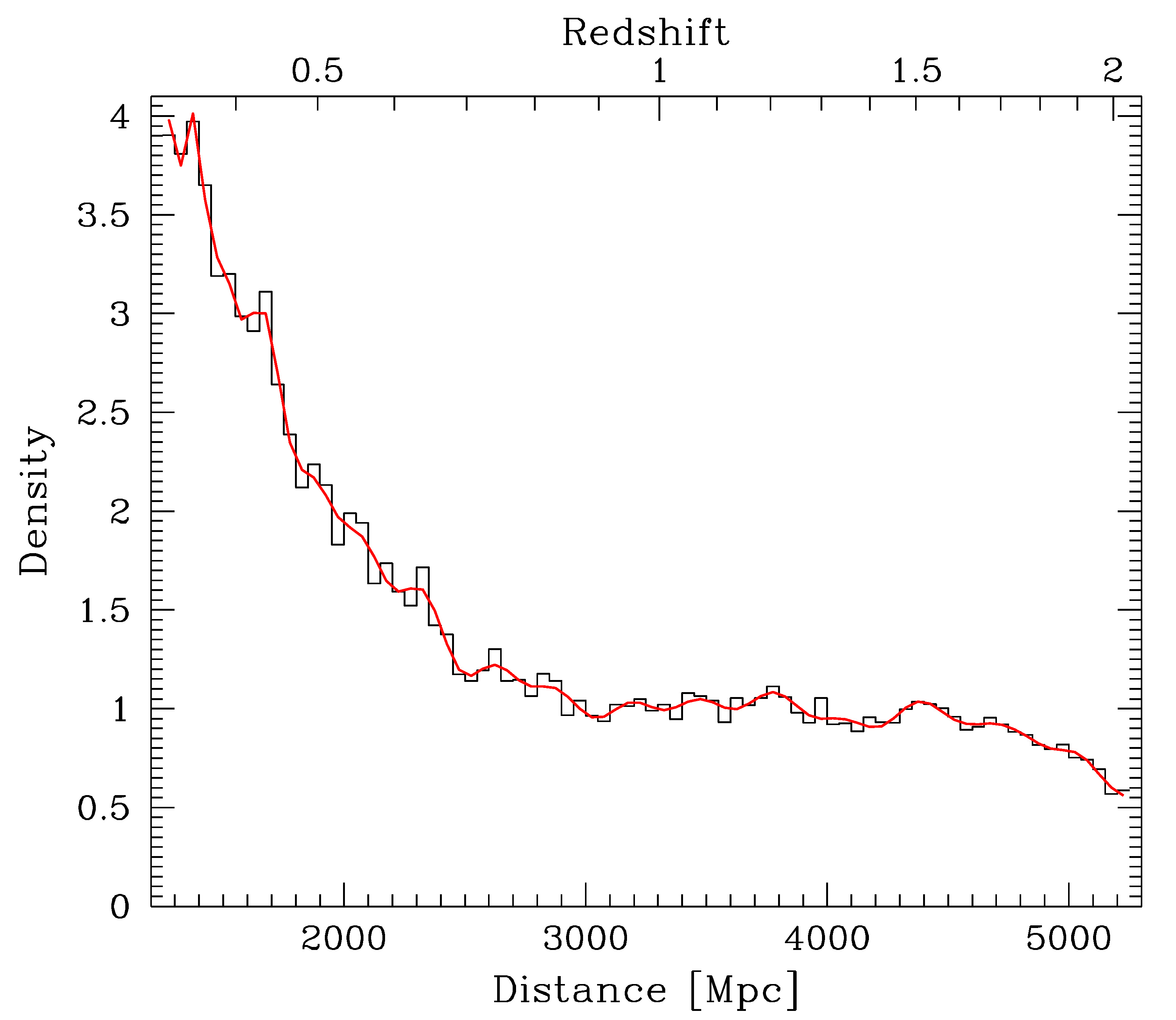
Figure 1: Distance distribution of quasar space density (arbitrary units) of the SDSS quasars brighter than $z=19.50$. Superimposed curve is a Legendre polynomial fit of degree $n=50$

.

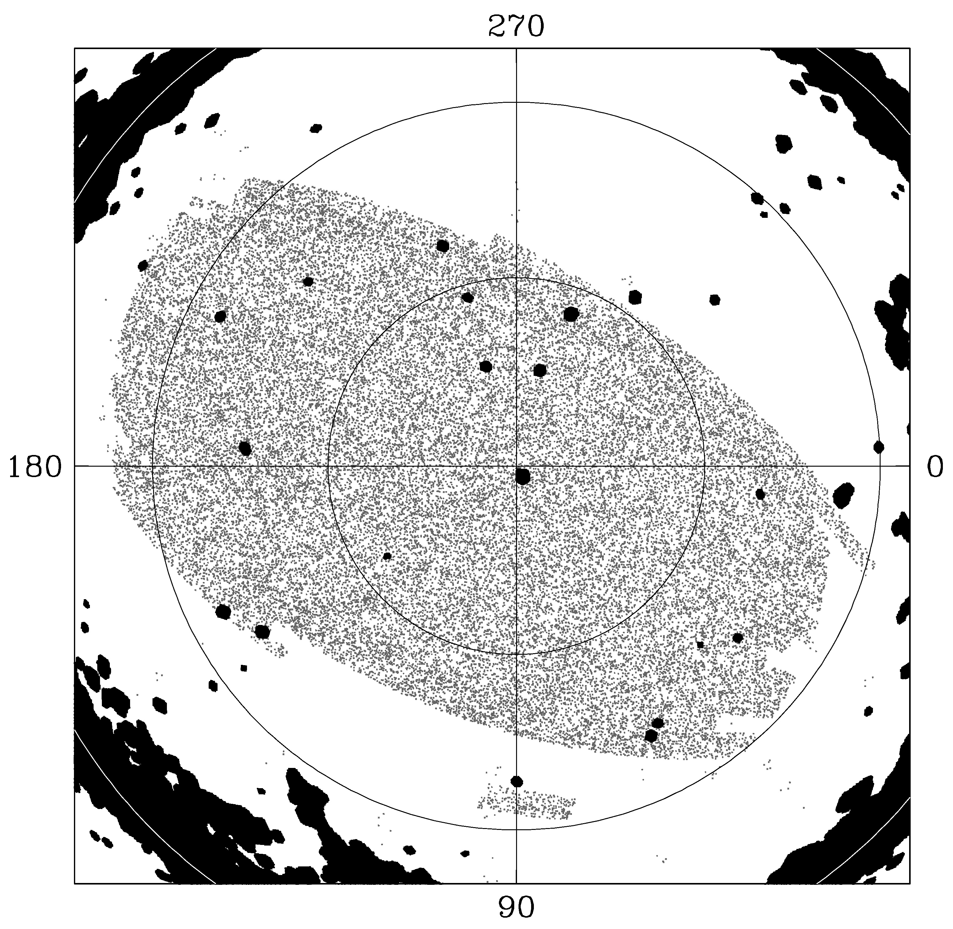
Figure 2: Distribution of $\sim 42400$ quasars brighter than $z=19.50$ in the north galactic hemisphere from the SDSS DR7 quasar catalogue at distances between $1300$ and $4700$ Mpc. Planck’s SEVEM mask is superimposed in black (see Sec. 2.2). Galactic latitude circles of $60^{\circ}$, $30^{\circ}$ and $0^{\circ}$ (arcs) are marked.

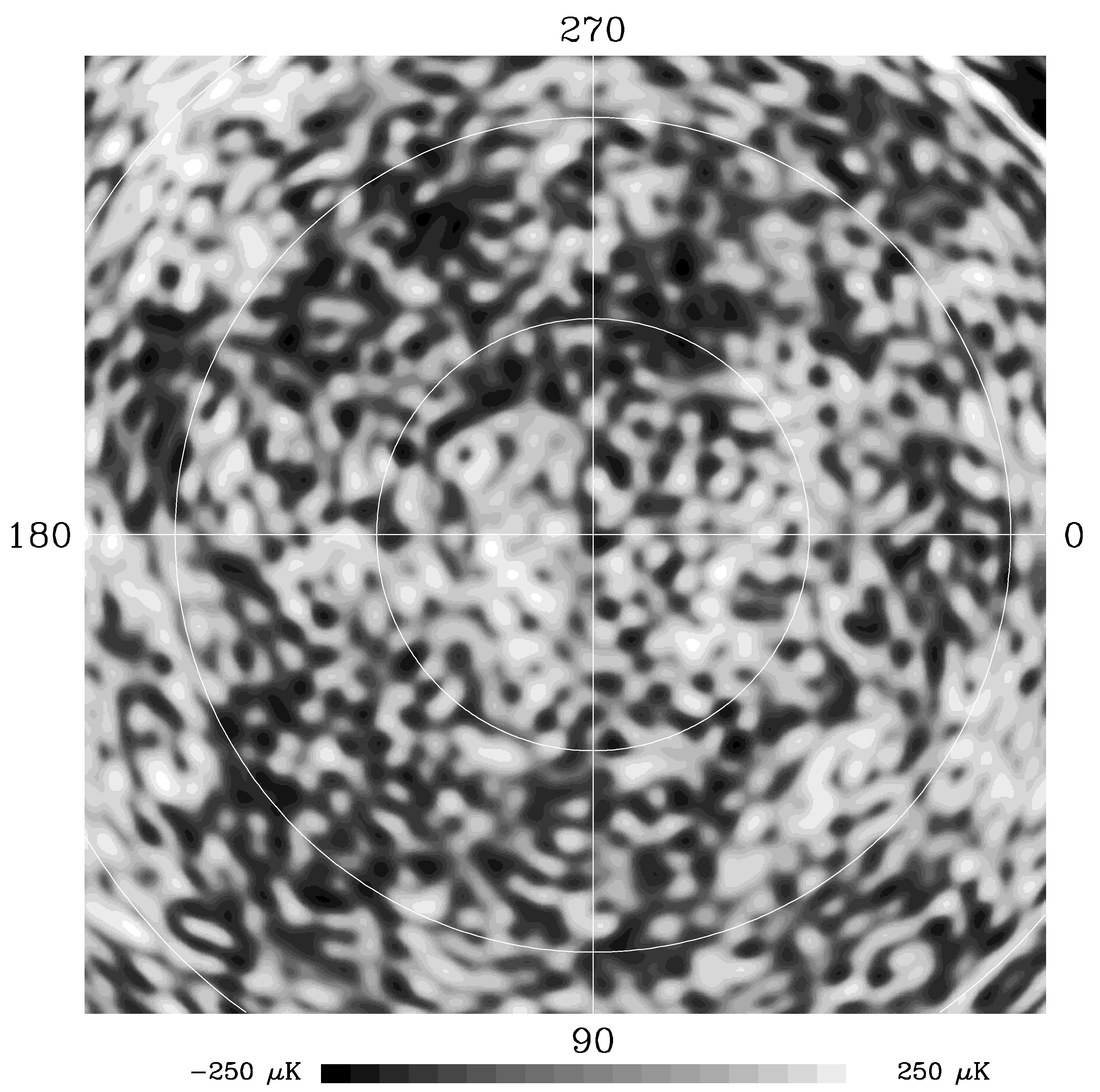
Figure 3: Spherical harmonic expansion of the Planck $2015$ SEVEM map in the north galactic hemisphere in polar projection (same area as Fig. 2) up to order $l=90$.

The Sloan Digital Sky Survey Quasar Catalogue covers a huge volume of space that allows for statistical investigation of the relationship between the large scale matter distribution and the fluctuations of the Cosmic Microwave Background (CMB) induced by the ISW effect. The fifth edition of this catalogue is described in detail by Schneider et al. (2010). All the procedures of the quasar selection, photometry and spectroscopic redshifts are presented in that paper. Here we summon only the overall parameters of the catalogue. We used the data in the north galactic hemisphere (NGH). Total number of quasars in this area exceeds $90\,000$. Additionally, we impose a rigid magnitude limit of $19.5$ in the $z$ band. Albeit, this $z$ cut-off decreases the number of quasars in the northern hemisphere to $\sim 70\,000$, it effectively reduces variations of the quasar surface density in the selected deep areas. Despite great effort to achieve statistical homogeneity of the catalogue, objects satisfying the selection criteria are subject to some residual biases discussed in detail by Schneider et al. (2010) (see also Sołtan 2017). In the present investigation we concentrate on the correlation between the quasar space distribution and the fluctuations of the CMB temperature. Admitting that various features of the catalogue generated locally in the process of the data acquisition increase the uncertainties of the final results, one can expect that these biases do not affect amplitudes of the cosmic signal. This conclusion applies also to our distance estimates. We ignore deviations from the Hubble flow and the distance is derived from the Hubble relationship in the considered cosmological model.

Distributions of quasars at distances between $1300$ and $5200$  Mpc ($0.33\lesssim z\lesssim 2.01$) is shown with the histogram in Fig. 1. The curve represents a fit by Legendre polynomial of degree $n=50$. The fit is used to generate quasi-random distribution of points using the MC method (see below). The catalogue is magnitude limited what introduces an overall gradient of object space density. Although, a strong cosmic evolution of quasars reduces to some extent the amplitude of this effect, the average space density of the catalogued objects at distance of $4500$ Mpc is $\sim 4$ times lower than at $1500$ Mpc. A wide plateau between $3000$ and $4500$ Mpc comes from a kind of interplay between the observational selection and the evolution. The distribution of the catalogued objects in the celestial sphere in galactic coordinates is shown in Fig. 2. A polar projection is used. Despite its featureless appearance, the subsequent analysis shows that the space distribution of objects is statistically nonuniform, and both concentrations of quasars and the under-dense regions reflect the large scale fluctuations of matter that in turn generate the ISW signal.

2.2 CMB map

The CMB temperatures data are based on the Planck 2015 data release (Planck Collaboration, 2016). Four maps: Commander, NILC, SEVEM and SMICA, that differ in methods of background subtraction are available. We use the SEVEM maps. One of the objectives of the SEVEM method was to minimize the variance of the clean map outside the confidence mask. This was achieved in a two step procedure. First, a set of template maps with removed the CMB signal was constructed. Then, a linear combination of templates was subtracted from the CMB-dominated maps. Since the expected amplitude of the ISW signal is substantially smaller than the integral fluctuations of the registered flux, the condition of minimum variance seems to be essential in our investigation. One should note also that in several investigations of the ISW effect, e.g. Planck Collaboration XIX (2014); Planck Collaboration XXI (2016); Nadathur & Crittenden (2016) the results using all the maps are very much alike. We used standard Res 10 HEALPix projection (Górski et al., 2005) with $\sim 3.4$ arcmin resolution. The NGH section of SEVEM data smoothed with the spherical harmonic filter of degree $l=90$ is shown in Fig. 3. In all calculations the confidence mask leaving approximately $85$ per cent of useful data has been applied. It is shown in Fig. 2.

3 Quasars and the ISW

3.1 The ISW effect in $\Lambda$CDM

Here we collect the formulae that describe effects of gravitational potential variations on the CMB photons in the low redshift Universe. We limit the analysis to the linear large-scale fluctuations of matter distribution in the $\Lambda$CDM model, known as the late-time Sachs-Wolfe effect. The temperature $T({\bf\hat{p}})$ of the CMB propagating in the direction defined by a unit vector $\bf\hat{p}$ deviates from the average temperature $\overline{T}$ (Dodelson, 2003, p. 238):

$$\frac{\delta T({\bf\hat{p}})}{\overline{T}}\,=\,\frac{T({\bf\hat{p}})-\overline{T}}{\overline{T}}\,=\,\frac{2}{c^{2}}\,\int_{\eta_{\rm LS}}^{\eta_{0}}{\rm d}\eta\;\frac{{\rm d}\Phi({\bf r},\eta)}{{\rm d}\eta}\,,$$ (1)

where $\eta$ is the conformal time, ${\rm LS}$ and $0$ denote the last scattering surface and the present moment, respectively; $\Phi({\bf r},\eta)$ is the distribution of the Newtonian gravitational potential along the photon path, ${\bf r}\,=\,{\bf\hat{p}}\,r$, where $r$ is comoving distance, and $c$ is speed of light.

Below we will model the gravitational potential distribution using the quasar sample, and it is convenient to rewrite Eq. 1 in the form:

$$\frac{\delta T({\bf\hat{p}})}{\overline{T}}\,=\,\frac{2}{c^{3}}\,\int_{0}^{r_{\rm LS}}{\rm d}r\,a\,\dot{\Phi}({\bf r},\,t)\,,$$ (2)

where $\bf{\hat{p}}$ is now unit vector defining direction in the sphere, $a=a(t)$ – scale factor of the universal expansion, and overdot denotes a time derivative.

In the matter-dominated flat Universe, i.e. with the critical density generated exclusively by matter, $\Omega_{\rm m}\,=\,1$, linear density fluctuations develop at the same rate as the scale factor $a$. Thus, the proper linear size of individual structure is proportional to its mass and gravitational potential does not evolve in time. Higher rate of the Universe expansion due to non-zero cosmological constant removes this degeneracy, and induces time evolution of $\Phi$.

A standard procedure to bind matter density fluctuations with the gravitational potential is to use the Poisson equation in Fourier space (e.g. Nadathur et al. 2012):

$$\Phi({\bf k},t)\,=\,-\frac{3}{2}\,H_{0}^{2}\,\Omega_{\rm m}\,\frac{\delta({\bf k},t)}{k^{2}\,a}\,,$$ (3)

where $\delta({\bf k},t)$ is the Fourier transform of the matter density fluctuations:

$$\delta({\bf r},t)\,=\,\frac{\rho({\bf r})-\overline{\rho}}{\overline{\rho}}\,.$$ (4)

The evolution of density fluctuations in the linear regime describes a growth factor $D(t)$: $\delta({\bf k},t)\,=\,D(t)\,\delta_{0}({\bf k})$. Time derivative of the Potential $\Phi$ is defined entirely by this function:

$$\dot{\Phi}({\bf k},t)\,=\,-\frac{3}{2}\,H_{0}^{2}\,\Omega_{\rm m}\,\frac{\delta_{0}({\bf k})}{k^{2}}\,\left[a\,\frac{{\rm d}D}{{\rm d}a}-D\right]\,\frac{\dot{a}}{a^{2}}\,,$$ (5)

and substituting $\beta(t)\,=\,{\rm d}\ln D/{\rm d}\ln a$ we get (Nadathur et al. 2012):

$$\dot{\Phi}({\bf k},t)\,=\,\frac{3}{2}\,H_{0}^{2}\,\Omega_{\rm m}\,\frac{H(t)}{a}\,\frac{\delta({\rm k},t)}{k^{2}}\,\left[1-\beta(t)\right]\,.$$ (6)

In the subsequent calculations, the relevant terms are derived for the $\Lambda$CDM cosmological model with parameters specified in the Introduction. The formulae for the linear growth rate, $D(t)$ were taken from Peebles (1980, p. 49–51).

If along the photon path there is a single spherically symmetric structure, the inverse transform of $\dot{\Phi}({\bf k},t)$ is given in a closed form:

$$\dot{\Phi}({\bf r},t)\,=\,\frac{3}{2}\,H_{0}^{2}\,\Omega_{\rm m}\,\frac{H(t)}{a}\,\left[1-\beta(t)\right]\,F(s)\,,$$ (7)

where $s$ is now distance form the structure centre, and

$$F(s)\,=\,\frac{1}{s}\,\int_{0}^{s}{\rm d}s^{\prime}\,{s^{\prime}}^{2}\,\delta(s^{\prime},t)\,+\,\int_{s}^{\infty}{\rm d}s^{\prime}\,s^{\prime}\,\delta(s^{\prime},t)\,.$$ (8)

In the linear case, the same formalism may be applied to the set of (spherical) objects distributed along the line of sight. In this case, the density profile $F(s)$ is replaced by a sum of profiles that represent separate structures. Albeit complexity of the cosmic matter distribution is not adequately represented by such simple arrangements, we are going to adapt the above formula in order to seek the correlation between the quasar distribution and the CMB map. In the following section we construct a simple statistics using the spatial distribution of quasars. Although, it cannot serve as the estimator of the gravitational potential, it is correlated with the potential. Then, this statistics is substituted into Eqs 7 and 8, and integrated according to Eq. 2.

3.2 Quasar statistics vs. CMB temperature fluctuations

A problematic application of the quasar sample to the investigation of the ISW effect depends on the relationship between the two highly disparate distributions: discrete, scarce quasar population and continuous gravitational potential. If a mean separation between the tracer objects is comparable or smaller than the interesting linear scale of potential variations, then the matter density field may be efficiently reconstructed using the Voronoi tessellation technique applied to the discrete data (e.g. van de Weygaert & Schaap 2009). This method was effectively utilized by by Granett et al. (2009), who modelled the potential using a sample of $400\,000$ galaxies at $z\sim 0.5$ from the SDSS (Adelman-McCarthy et al. 2008).

Nadathur et al. (2012) showed that within the linear approximation in the $\Lambda$CDM model, the ISW signal generated by numerous small and moderate size structures is much weaker than the primordial fluctuations of the CMB occurring at the surface of last scattering. It appears that only the superstructures of size $\sim\!100$ Mpc or larger produce signal that is statistically distinguishable from the background. The mean distance between the neighbouring galaxies in the Granett et al. (2009) investigation amounts to $\sim\!19$ Mpc. Thus, spatial resolution attainable by means of the Voronoi tessellation is adequate to estimate potential on the required scales. The mean distance in our quasar sample approaches $100$ Mpc at $z\,=\,0.5$ and increases to $124$ Mpc at $z\,=\,1$. Because of the much lower space density, the discrete nature of the distribution strongly affects the local density estimates. We assess that a less refined approach than the Voronoi tessellation would be adequate.

One can expect that Poisson noise in our sample will hamper an identification of individual superstructures in the quasar catalogue. Nevertheless, a relationship between large scale matter distribution and quasars exists still in the form of statistical correlation of the local number density of quasars with the total matter density. It implies that in the randomly selected volume of space, $V$, number of quasars is correlated with the total amount of matter contained in that volume. To keep a linear character of the correlation we make a standard assumption that a ‘quasar bias factor’, i.e. the ratio of the relative overdensities of quasars to total matter is constant in statistical sense. The amplitude of this correlation, or correlation coefficient, depends critically on space density of quasars, and it is expected to be strongly reduced by the stochastic nature of the Poisson distribution. Keeping in mind this limitation, we define the amplitude of quasar space density variations the same way as the total matter density fluctuations:

$$\delta\nu\,=\,\frac{n_{\rm o}-n_{\rm f}}{n_{\rm f}}\,,$$ (9)

where $n_{\rm o}$ and $n_{\rm f}$ are the observed and average number of quasars in $V$. Because of a strong radial density gradient in our quasar sample, excess or deficiency of quasars is normalized to the average number of quasars expected for given distance, $n_{\rm f}=n_{\rm f}(D)$. The average number is determined using the Lagrange fit shown in Fig. 1. In all the following considerations, the test volume $V=V(r_{\rm s})$ is a sphere, and the interesting correlations will be investigated over a wide range of the sphere radii, $r_{\rm s}$.

In Fig 4 we show two typical distributions of quasars between $1500$ Mpc and $4500$  Mpc. At each point objects are counted within a sphere of $100$ Mpc radius. Plots exemplify typical patterns observed in the catalogue. Upper panel gives the actual numbers of observed objects, what illustrates importance of the Poisson scatter.

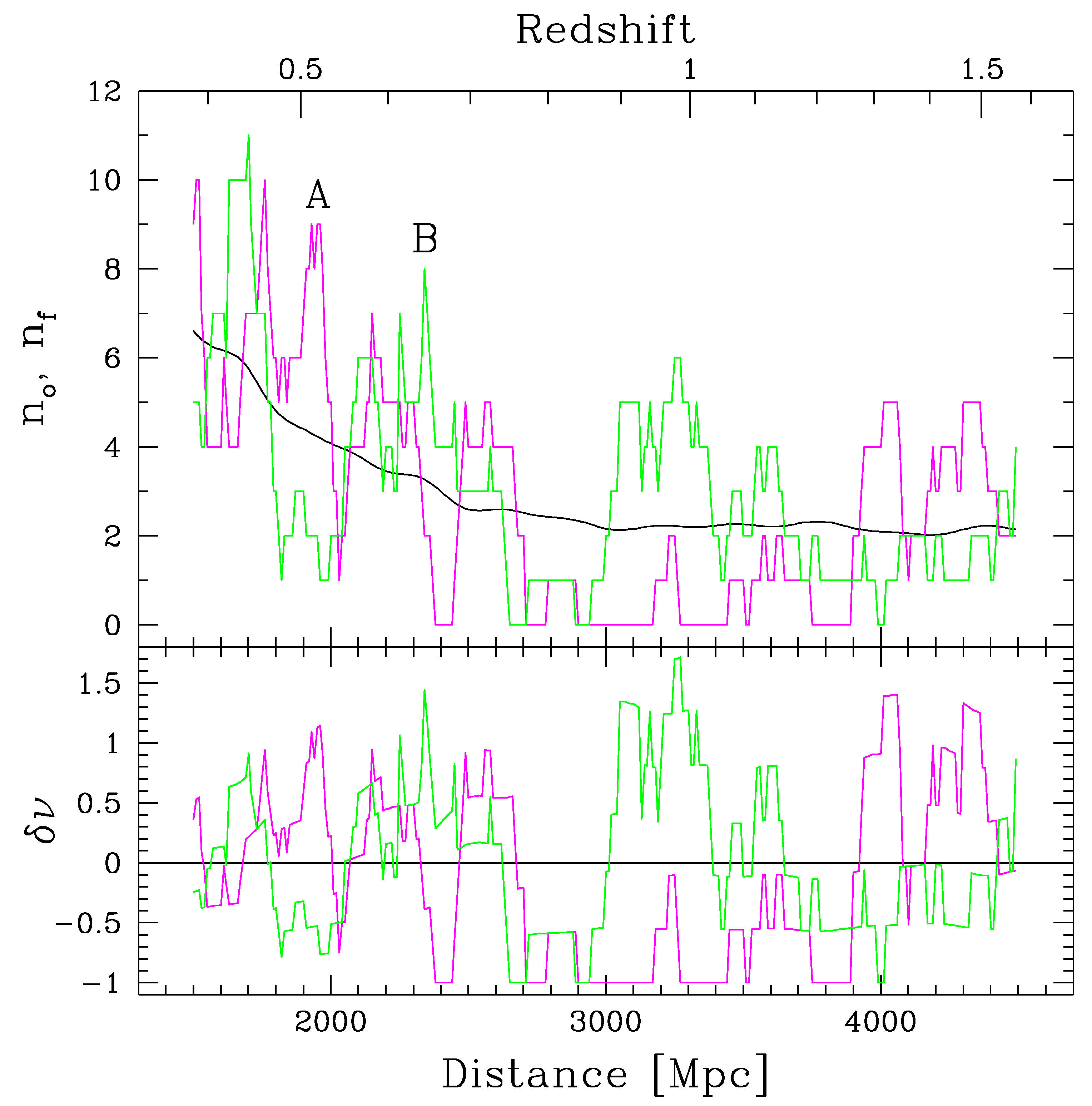
Figure 4: Two typical radial distributions of quasars along radial directions: A($l=58^{\circ},b=50^{\circ}$) and B($l=236^{\circ},b=60^{\circ}$), for sphere radius $r=100$ Mpc (see text). Upper panel: observed numbers of quasars, $n_{\rm o}$ (erratic curves), and the average number based on the Legendre fit, $n_{\rm f}$. Lower panel: relative fluctuations of quasar concentration as defined in Eq. 9.

Cosmological simulations allow to relate distribution of tracing objects, with the total matter density, then - with the structure of the gravitational potential, and the ISW effect (e.g. Watson et al. 2014; Nadathur et al. 2017). Observational data do not provide such gratifying information. Therefore we seek for a direct empiric relationship between the quasar distribution and the ISW signal. It is evident that the $\delta\nu$ parameter constitutes a poor indicator of the potential. We notice, however, that under the assumption of the constant quasar bias factor, the gravitational potential $\Phi({\bf r},t)$ along the photon path is correlated with the distribution of $\delta\nu=\delta\nu({\bf r})$. In the linear approximation the potential is also linearly correlated also with the local matter density fluctuation averaged over a sphere of finite radius $r_{\rm s}$. Since the CMB temperature variations are related to $\Phi({\bf r},t)$ via Eq. 2, one can expect also the correlation between $\delta\nu$ and $\delta T$. One should emphasize that no definite relationship between $\delta\nu$ and $\Phi({\bf r},t)$ or $\delta T$ is assumed. In particular, the quasar bias factor is not present in the calculations.

As we are interested in the impact of the variations of the matter distribution on the CMB, one should consider the matter density fluctuations over the whole section of the photon paths within the selected volumes. Accordingly, we define the ‘net’ density deviation between distances $D_{\rm l}$ and $D_{\rm h}$ as:

$$\Delta N\,=\,\frac{1}{D_{\rm h}-D_{\rm l}}\,\int_{D_{\rm l}}^{D_{\rm h}}\delta\nu\,{\rm d}D\,.$$ (10)

One can expect that the distribution of the $\Delta N$ over the sky should correlate with the ISW signal. Thus, $\Delta N$ should also correlate with with the total CMB variations. Yet, the functional relationships between the matter density distributions and the gravitational potential given in Eqs. 7 and 8 indicate that the stronger correlation is expected when the local density fluctuation $\delta\nu$ is substituted into Eq. 7 instead of $F(s)$. The modified form of Eq. 7 is substituted into Eq. 2, that defines a new parameter $\Delta Q$ is as follows:

$$\Delta Q\,=\,3\,\frac{\overline{T}}{c^{3}}\,H_{0}^{2}\,\Omega_{\rm m}\int_{D_{l}}^{\rm D_{h}}{\rm d}r\,H(t)\left[1-\beta(t)\right]\,\delta\nu\,.$$ (11)

Both $\Delta N$ and $\Delta Q$ are defined as the averaged density fluctuations $\delta\nu$. The $\Delta N$ is a simple arithmetic average over distance, while in $\Delta Q$ the fluctuations are weighted in the same way as the gravitational potential in the ISW effect. Although amplitude $\Delta Q$ is measured in $\mu$K, this quantity should not be treated as the estimate of the ISW effect generated by the matter distribution between $D_{\rm l}$ and $D_{\rm h}$. $\Delta Q$ is a variable functionally dependent on the quasar distribution, and as such it is expected to correlate with the the ISW signal.

We analyze three subsets of the quasar catalogue: the whole data between $D_{\rm l}=1500$ Mpc and $D_{\rm h}=4500$ Mpc, and separately quasars in two distance bins: $1500-3000$ Mpc and $3000-4500$ Mpc. To assess the correlation coefficient between $\Delta Q$ and $\delta T$, we consider a dense net of equally spaced pointings over the area covered by the SDSS quasar catalogue. Spacing between pointings was selected at $\theta=60$ arcmin (see below). For each pointing the amplitudes of $\Delta Q$ and the CMB temperature signal are calculated. Geometric settings for the data acquisition are shown in Fig. 5. The quasar relative density variations, $\Delta Q$, are determined between the distances $D_{\rm l}$ and $D_{\rm h}$. A question of the angular extent of the individual $\delta T$ measurement is not well-defined. First, the definition of $\Delta Q$ variable neither determines the characteristic angular scale for the gravitational potential variations, nor defines the optimal shape of the filter. Second, $\Delta Q$ is determined using fixed volume $V=V(r_{\rm s})$ at a wide range of distances.

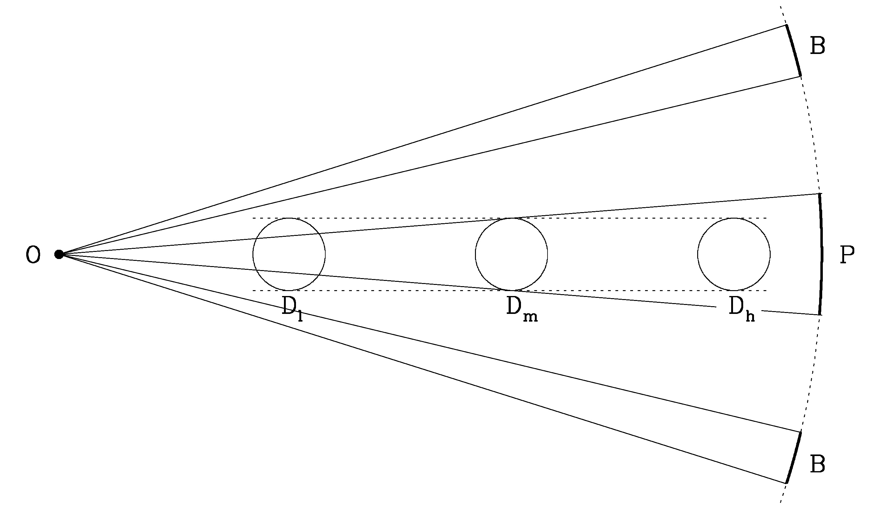
Figure 5: Schematic view indicating configuration of the areas used to determine amplitudes $\Delta N$ i $\delta T$ for a single pointing. Quasars within a 3D volume swept through by the sphere moving between $D_{\rm l}$ and $D_{\rm h}$ contribute to the $\Delta N$ estimate, while 2D areas ‘P’ and ‘B’ are used to determine $\delta T$ fluctuation (see text).

With no direct constraints on the optimal size for the temperature evaluation area, we take a 2D Gaussian function parametrized by variance $\sigma_{\rm P}^{2}$. It is reasonable to assume that the angular scale of $\delta T$ estimates should correspond to the ‘average’ angular size of the area used to calculate $\Delta Q$. This is because the area of the highest amplitude of the ISW signal roughly coincides with the structure size. A radius of this ’reference’ area (denoted $P$ in Fig. 5) $\vartheta=r_{\rm s}/D_{\rm m}$, where $D_{\rm m}$ is the median distance between $D_{\rm l}$ and $D_{\rm h}$. Consequently, the temperature assigned to the pointing is the average temperature weighted with the Gaussian function of width $\sigma_{\rm P}$. Geometrical settings are insufficient to specify $\sigma_{\rm P}$ and it is considered a free parameter. In the calculations several values of $\sigma_{\rm P}$ were adopted within a range

$$0.2\,\vartheta\,\leq\,\sigma_{\rm P}\,\leq\,1\,\vartheta\,,$$ (12)

The radius of the integration area was assumed at $3\,\sigma_{\rm P}$ for each $\sigma_{\rm P}$.

To minimize the large angular scale temperature variations uncorrelated with $\Delta Q$, $\delta T$ is defined as a difference between the temperature in the pointing direction and in the surrounding area (denoted by B in Fig. 5), defined as a ring centered on given pointing with the inner radius $\theta_{\rm in}\,=\,\max[1.5\,r_{\rm s}/D_{\rm l},\,3\,\sigma_{\rm P}]$ , and width of $4$ deg. Thus, procedure to determine $\delta T$ corresponds to the use of Mexican hat filter with flat negative section. All the calculations were performed for sphere radii between $40$ and $140$ Mpc.

4 Contribution of the ISW effect to the CMB maps

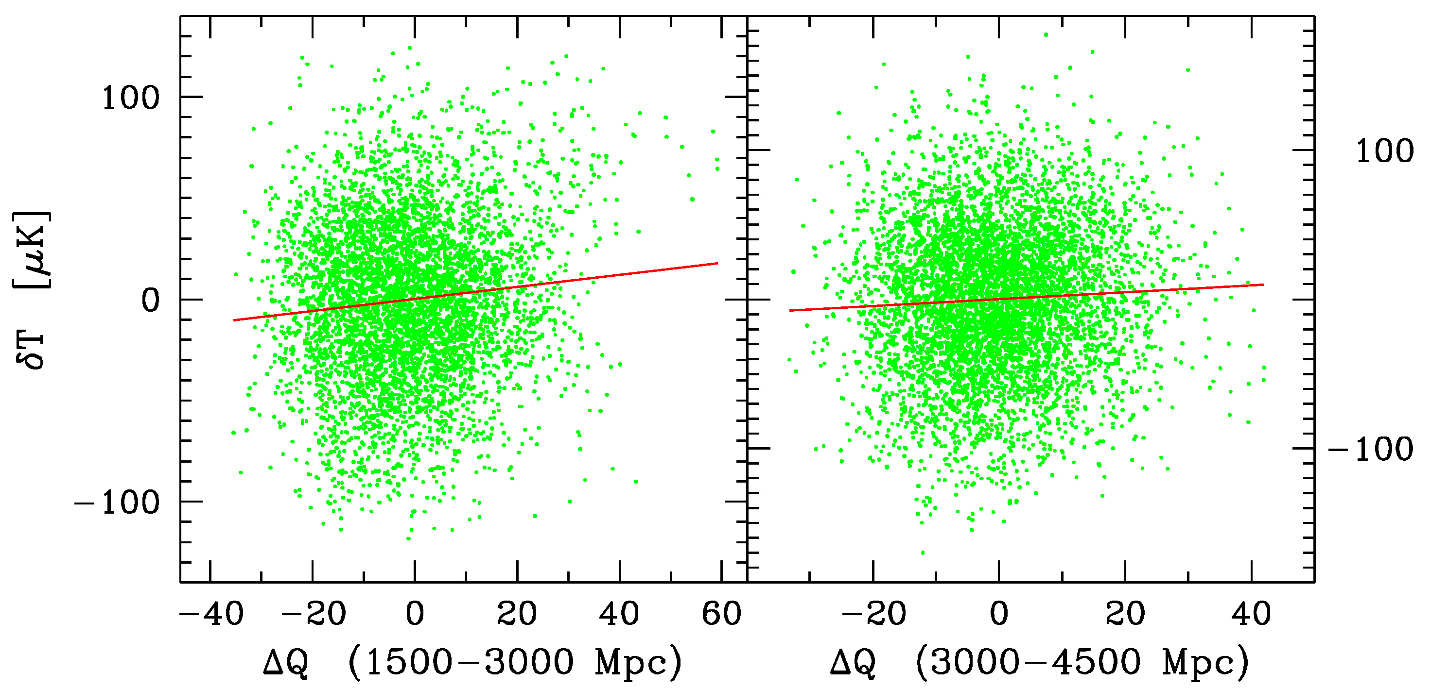
Figure 6: Distributions of local temperature amplitude and the quasar excess density in the distance bin $1500-3000$ Mpc (left panel), and $3000-4500$ Mpc (right panel) for spheres of radius $r_{\rm s}=100$ Mpc, and $\sigma_{\rm P}=0.4\,\vartheta$ in more than $5000$ pointings (see text). Tilted lines are the least square best fits of $\delta T$ on $\Delta Q$.

High concentrations of pointings caused by their small separations ensured efficient exploitation of all the features of the QSO catalogue. Total number of useful pointings, $N_{\rm pnt}$, i.e. pointings not affected by the mask, and sufficiently distant from the survey edges to warrant correct $\delta\nu$ counts, depends on the minimum distance, $D_{\rm l}$, and the sphere radius, $r_{\rm s}$. For $D_{\rm l}=1500$ Mpc and $r_{\rm s}=40$ Mpc it exceeds $5600$, and drops to $\sim 4500$ for $r_{\rm s}=140$ Mpc. In Fig. 6 we plot the local temperature fluctuation, $\delta T$, for $\sigma_{\rm P}=0.4\,\vartheta$, against the relative density excess, $\Delta Q$, in more than $5000$ pointings for two distance bins $D_{\rm l}-D_{\rm h}$: $1500-3000$ Mpc and $3000-4500$ Mpc, for $r_{\rm s}=100$ Mpc. The data are positively correlated. The Pearson correlation coefficients $\rho=0.0992$ and $0,0528$ for the low and high distance bin, respectively. For the merged data, i.e. between $1500$ and $4500$ Mpc the correlation coefficients amounts to $0.1082$. We calculated also correlation coefficients for the $\delta T-\Delta N$ distribution. In agreement with the reasoning above, the figures in this case are systematically lower, but the differences are insignificant. For the low, high and merged distance bins the corresponding coefficients are $0.0933$, $0.0522$ and $0.1038$, respectively.

Although the cloud of points is adequately represented by a 2D Gaussian distribution, a significance of the correlation is not given by standard statistical formulae applicable for the Gaussian function. Because of tight pointing spacing, the amplitudes $\Delta Q$ are not independent variables, and the uncertainty range of $\rho$ has to be assessed separately using the MC simulations.

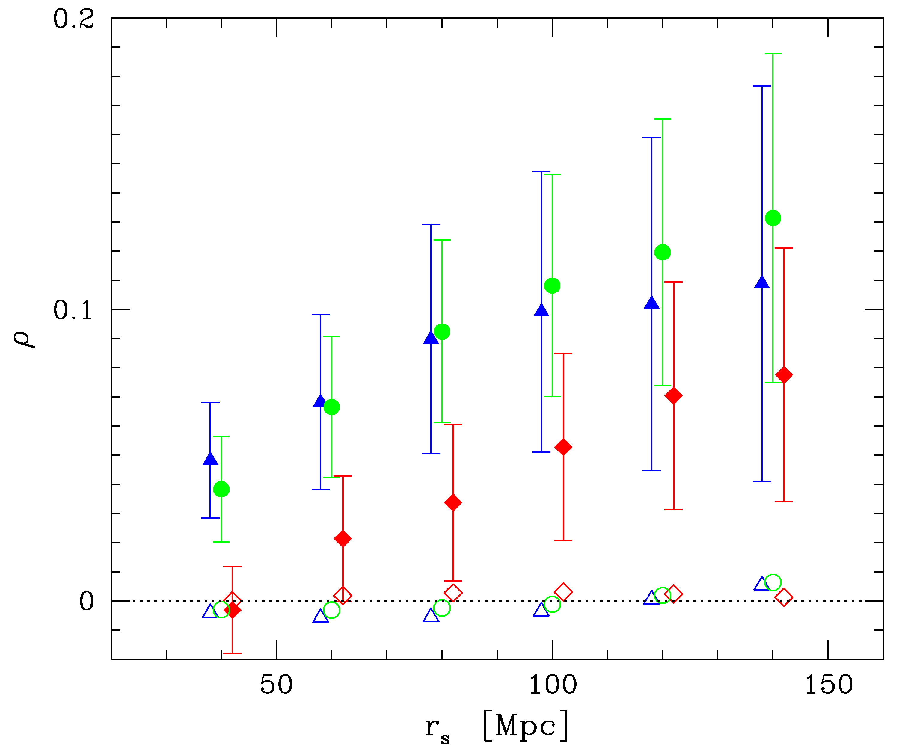
Figure 7: The Pearson correlation coefficient, $\rho_{\rm N}$, between $\delta T$ for $\sigma_{\rm P}=0.4\,\vartheta$, and $\Delta N$ in the distance bin $1500-3000$ Mpc (full triangles), $3000-4500$ Mpc (full squares), and $1500-4500$ Mpc (full circles) for a range of sphere radii $r_{\rm s}$; error bars represent rms scatter of the correlation coefficients computed for $55$ sets of mock data (see text). Open symbols - average coefficients computed for the mock data.

We calculate correlation coefficients for a large number of the mock data. The SDSS QSO and CMB temperature maps are shifted against each other to erase the physical correlation. The rms scatter of the residual correlation signal calculated for combined map pairs is taken as representing the statistical noise of our estimate of $\rho$. To get sufficiently large number of combined map pairs the following procedure is applied. First, we rotate the quasar data in $15^{\circ}$ steps about the axis $(l,b)=(120^{\circ},0^{\circ})$. In galactic coordinate system it shifts quasars at the north galactic pole in Fig. 2 south along longitude of $30^{\circ}$. This method generates $23$ sets of uncorrelated quasar and CMB maps. Then, the quasar data are rotated by $60^{\circ}$ about the galactic polar axis and the procedure to rotate the map in $15^{\circ}$ steps, this time about $(l,b)=(120^{\circ},0^{\circ})$ axis, is repeated. Finally, the quasar data are rotated by $120^{\circ}$ about the galactic polar axis and $15^{\circ}$ step map multiplication about $(l,b)=(180^{\circ},0^{\circ})$ axis is executed. This scheme generates in total $69$ data sets. For most of data pairs some pointings fall in the masked area in the SEVEM map. If more than half of the area used to estimated $\delta T$ is masked out, the pointing is not used. Therefore the correlation coefficients of the test data are determined using the smaller number of pointings. For this reason, estimates of the $\rho$ rms get larger above the level expected for the real data. To lessen this effect, the rms was calculated using only the test maps with the number of accepted pointings larger than $75$ per cent of pointings used in the real data. Removal of heavily masked maps had minimal effect on error estimates. Within the considered range of all the parameters the number of the test data sets used in the error estimates has not dropped below $54$.

In Fig. 7 we plot the $\delta T-\Delta Q$ correlation coefficients in all three distance bins for a range of sphere radii. The error bars are estimated using the mock data sets. For all the combinations of parameters, the correlations are positive. However the signal in the $3000-4500$ Mpc bin is substantially weaker and never exceeds $2\,\sigma$. In the full distance range of $1500-4500$ Mpc the positive $\delta T-\Delta Q$ correlation is significant above $2.5\,\sigma$ for the sphere radii $50\leq r_{\rm s}\leq 120$ Mpc. The data divided into low and high distance bins show weaker correlation significance but in the $1500-3000$ Mpc bin within the range $40\leq r_{\rm s}\leq 100$ Mpc it still exceeds $2\,\sigma$.

Moderate, but measurable correlations between $\delta T$ and $\Delta Q$ provide intriguing constraints on the amplitude of the ISW effect produced by the matter accumulated between $D_{\rm l}$ and $D_{\rm h}$. For the purpose of the present analysis the total observed temperature deviation from the average, $\delta T$, is a sum of four components: primordial fluctuations generated in the recombination era, the ISW effect produced in the $D_{\rm l}-D_{\rm h}$ distance range, the ISW outside these distances, and measurement errors. Clearly, only the ISW effect generated between $D_{\rm l}-D_{\rm h}$ can correlate with $\Delta Q$. Thus, the temperature fluctuations $\delta T$ may be decomposed into two statistically independent parts: $\delta T\,=\,\delta T_{\rm un}+\delta T_{\rm cr}$, uncorrelated and correlated with the $\Delta Q$, respectively.

Let $t$ and $q$ denote the amplitudes of $\delta T$ and $\Delta Q$ for individual pointings. In Appendix A we recall canonical relationships between standard deviations of the linearly correlated variables, and apply the respective formulae to the quantities $\sigma_{\rm t}$ and $\sigma_{\rm q}$. We find also the relationship between these quantities and the standard deviation of the ISW effect. The relationships are obtained under the assumption that the variables $t$ and $q$ have the averages $\mu_{\rm t}$ and $\mu_{\rm q}$ equal to zero and the Pearson correlation coefficient $\rho_{\rm tq}\neq 0$.

The ISW effect induced by the matter density fluctuations between $D_{\rm l}$ and $D_{\rm h}$ generates the rms temperature fluctuations, $\sigma_{\rm s}$ that contribute to the total CMB temperature variations $\sigma_{\rm t}$. According to Eq. 19, the variance $\sigma_{\rm s}^{2}$ is a sum of two positive components: $\sigma_{s|c}^{2}$ and $\sigma_{\rm o}^{2}$, where the former term, $\sigma_{s|c}$, represents the scatter that is not directly observable (see Appendix A), while the latter one can be determined from the data. Therefore, the present method provides the lower limit for the ISW effect (Eq. 20):

$$\sigma_{\rm s}\,>\,\sigma_{\rm o}\,=\,\rho_{\rm tq}\,\frac{\sigma_{\rm t}\,\sigma_{\rm q}}{\sqrt{\sigma_{\rm q}^{2}\,-\,\sigma_{\rm r}^{2}}}\,,$$ (13)

where $\sigma_{\rm r}$ represents a contribution to the $\sigma_{\rm q}$ generated by stochastic nature of the discrete quasar data. The amplitude of variable $\sigma_{\rm r}$ is determined by the Poisson statistics. Consequently, $\sigma_{\rm r}$ is correlated neither with the ISW effect nor the total CMB fluctuations. To assess $\sigma_{\rm r}$, a large number of the mock quasar data were generated using the Monte Carlo scheme in which the spherical coordinates were randomized while the radial coordinate of points were drawn from the probability distribution function based on the fit shown in Fig. 1. Equation 13 provides limits for the ISW effect based on correlations in sky coordinates. Its counterpart in the harmonic space are given by Granett et al. (2009). The lower bound rather than the actual amplitude of the ISW signal results from the fact that no definite relationship between the gravitational potential and the quasar distribution has been used.

In Fig. 8 we plot the $\sigma_{\rm o}$ amplitudes in the distance bins $1500-3000$ Mpc, $3000-4500$ Mpc and $1500-4500$ Mpc, for $\sigma_{\rm P}=0.4\vartheta$ and several sphere radii, $r_{\rm s}$. The error bars are derived from the MC simulations in a similar way as the rms uncertainties of coefficient $\rho$. In Table 1 a selection of the relevant parameters are listed for sphere radii, $r_{\rm s}$, in the range of $50-110$ Mpc. The amplitude of $\sigma_{\rm o}$ as a function of the width of the filter applied to compute the temperature variations, $\sigma_{\rm P}$, is plotted in Fig. 9. We recall that the amplitudes plotted in figures represent just a fraction of the variance $\sigma_{\rm o}^{2}$ that is ‘explained’ by the model (see the Appendix). Variations of $\sigma_{\rm o}$ for different sphere radii reflect variations of the ‘unexplained’ fraction of $\sigma_{\rm s}$ or, equivalently, an effectiveness of $\Delta Q$ function to trace the gravitational potential.

Albeit, the present calculations probe a wide range of linear scales, a shape of the $\sigma_{\rm o}$ variations does not define any particular characteristic scale of the gravitational potential fluctuations. Smooth distributions of $\sigma_{\rm o}$ against $r_{\rm s}$ and $\sigma_{\rm P}$ indicated in Figs. 8 and 9 shows that the $\Delta Q$ parameter correlates with the potential for a wide range of sphere radii. At the same time, it demonstrates ability of the present method to impose restrictive lower limit on the amplitude of the ISW signal. One should also notice that the high amplitude of $\sigma_{\rm o}$ is not associated with any exceptional statistical anomaly.

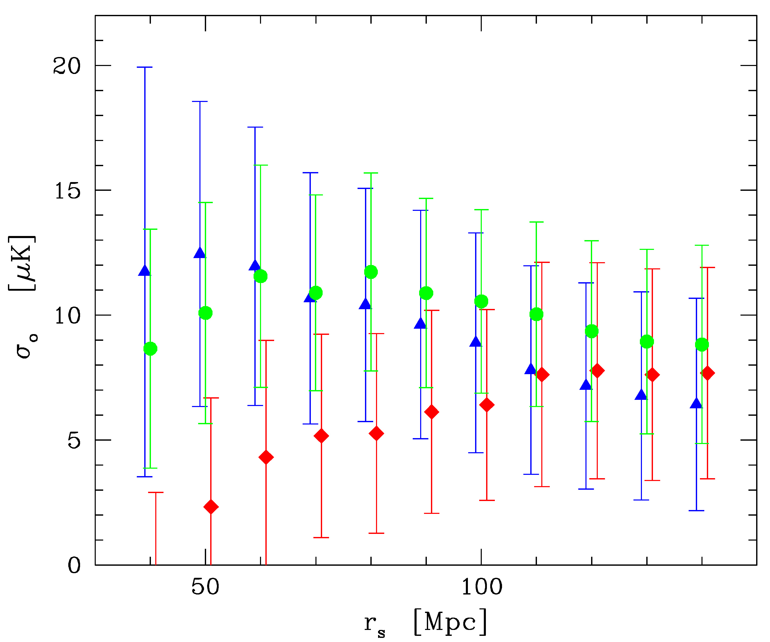
Figure 8: Observational lower limits for the rms fluctuations of the ISW signal (Eq. 20) for distances $D_{\rm l}-D_{\rm h}=1500-3000$ Mpc (triangles), $3000-4500$ Mpc (diamonds), and $1500-4500$ Mpc (dots), for sphere radii $40\leq r_{\rm s}\leq 140$ Mpc, and the filter parameter $\sigma_{\rm P}\,=\,0.4\,\vartheta$ (Eq. 12).

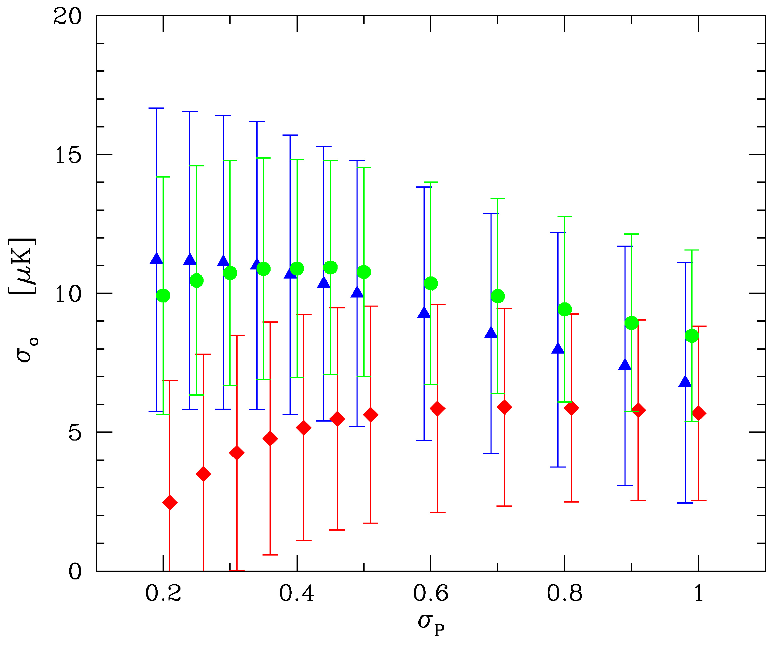
Figure 9: Observational lower limits for the rms fluctuations of the ISW signal (Eq. 20) for distances $D_{\rm l}-D_{\rm h}=1500-3000$ Mpc (triangles), $3000-4500$ Mpc (diamonds), and $1500-4500$ Mpc (dots), for a range of filter parameters $0.2\,\vartheta\leq\sigma_{\rm P}\leq 1\,\vartheta$ (Eq. 12), for the sphere radius $r_{\rm s}\,=\,70$ Mpc.

High amplitude of temperature fluctuations generated at the last scattering surface introduce a strong noise to our $\sigma_{\rm o}$ estimates. Therefore uncertainties of single results are in most cases large, what prevents us from definite particular conclusions. Still, some general tendencies are visible.

Both the near and distant samples give positive $\delta T-\Delta Q$ correlations and provide some constraints on the ISW effect. However, the relationships between the $\sigma_{\rm o}$ and $r_{\rm s}$ in these samples are different. In the near sample ($1500-3000$ Mpc) the $\sigma_{\rm o}$ amplitudes are relatively high at small sphere radii and diminish with increasing $r_{\rm s}$. The effect is likely caused by the overall quasar distribution in the sample. Strong radial density gradient introduces a bias to quasar counts in spheres, and the effect is dominating for large $r_{\rm s}$. The opposite tendency is present in the distant sample ($3000-4500$ Mpc) with roughly stable quasar density. In such setting the Poissonian fluctuations are the main source of noise, and their effect on counts is less pronounced for larger spheres.

Table 1: Interesting parameters on the $\Delta Q-\delta T$ correlations for $\sigma_{\rm P}=0.4\vartheta$, in distances $1500-3000$ Mpc and $1500-4500$ Mpc.

(1)	(2)	(3)	(4)	(5)
$r_{\rm s}^{a}$	$\rho$	$\sigma_{\rm o}^{b}$	$\rho$	$\sigma_{\rm o}^{b}$
	$[1500-3000]$		$[1500-4500]$
$~{}50$	$0.059\pm 0.025$	$12.4\pm 6.1$	$0.053\pm 0.021$	$10.1\pm 4.4$
$~{}60$	$0.068\pm 0.030$	$12.0\pm 5.6$	$0.066\pm 0.024$	$11.6\pm 4.5$
$~{}70$	$0.077\pm 0.034$	$10.7\pm 5.0$	$0.077\pm 0.027$	$10.9\pm 3.9$
$~{}80$	$0.090\pm 0.039$	$10.4\pm 4.7$	$0.092\pm 0.031$	$11.7\pm 4.0$
$~{}90$	$0.092\pm 0.044$	$~{}9.6\pm 4.6$	$0.099\pm 0.035$	$10.9\pm 3.8$
$100$	$0.099\pm 0.048$	$~{}8.9\pm 4.4$	$0.108\pm 0.038$	$10.6\pm 3.7$
$110$	$0.102\pm 0.052$	$~{}7.8\pm 4.2$	$0.116\pm 0.042$	$10.0\pm 3.7$

$a$ - in Mpc, $b$ - in $\mu$K.

5 Discussion

The average number of quasars in the SDSS catalogue found within a sphere of radius $r_{\rm s}\,=\,100$ Mpc varies from $6.6$ at distance $1500$ Mpc to $2.2$ at $3000$ Mpc, and $2.1$ at $4500$ Mpc. Thus, the Poisson noise strongly perturbs estimates of the average matter density, particularly at smaller $r_{\rm s}$ (see also Nadathur et al. 2017). It effectively precludes attempts to directly estimate space distribution of gravitational potential. Instead we define the parameter, $\Delta Q$, determined by the quasar space distribution, that is statistically correlated with the potential. We then measure the $\delta T-\Delta Q$ correlation amplitude to determine $\sigma_{\rm o}$ – a fraction of the temperature fluctuations that can be explained by this correlation. The signal characterized by $\sigma_{\rm o}$ constitutes the lower limit for total fluctuations generated between $D_{\rm l}$ and $D_{\rm h}$. In the calculations, the origin of the correlation is not decided. Albeit, it is natural to interpret the signal within the framework of the ISW effect.

The amplitude of the CMB rms fluctuations derived from the $\delta T-\Delta Q$ correlation, or the lower limit of the ISW effect, $\sigma_{\rm o}$, is determined with limited accuracy. For the distant sample a significance of the measurement does not exceed $2\sigma$, Thus, taken at its face value, the distant sample is consistent with no ISW signal. However, the near and distant samples combined together give the significance of the detection higher than each sample separately. For $r_{\rm s}=80$ Mpc the correlation coefficient $\rho=0.0924$ differs from zero at $2.9\,\sigma$. The correlations in the near sample alone exceed $2\,\sigma$ for $r_{\rm s}$ between $40$ and $100$ Mpc.

In this context, a couple of findings in the present investigation are to some extent surprising. The $\delta T-\Delta Q$ correlations show a posteriori that quasar number counts in spheres provide descriptive assessments on the gravitational potential along the line of sight, and constrain the amplitude of the ISW effect. More numerous sample of objects would allow to model the space distribution of the potential and to reduce the shot noise. Presumably, a correlation of such new statistics with $\delta T$ would impose still stronger constraints.

Magnitude of the ISW effect depends on the parameter $1-\beta(t)$ in Eq. 7. For the assumed $\Omega_{\Lambda}$ and $\Omega_{\rm m}$ in the $\Lambda$CDM model, $1-\beta(t)$ rises with decreasing redshift (see Fig 10). Our results qualitatively reflect this tendency. The most significant estimates of $\sigma_{\rm o}$ for the near bin are higher than the best estimate for the distant bin. However, sizable uncertainties prevent us from any definite conclusions.

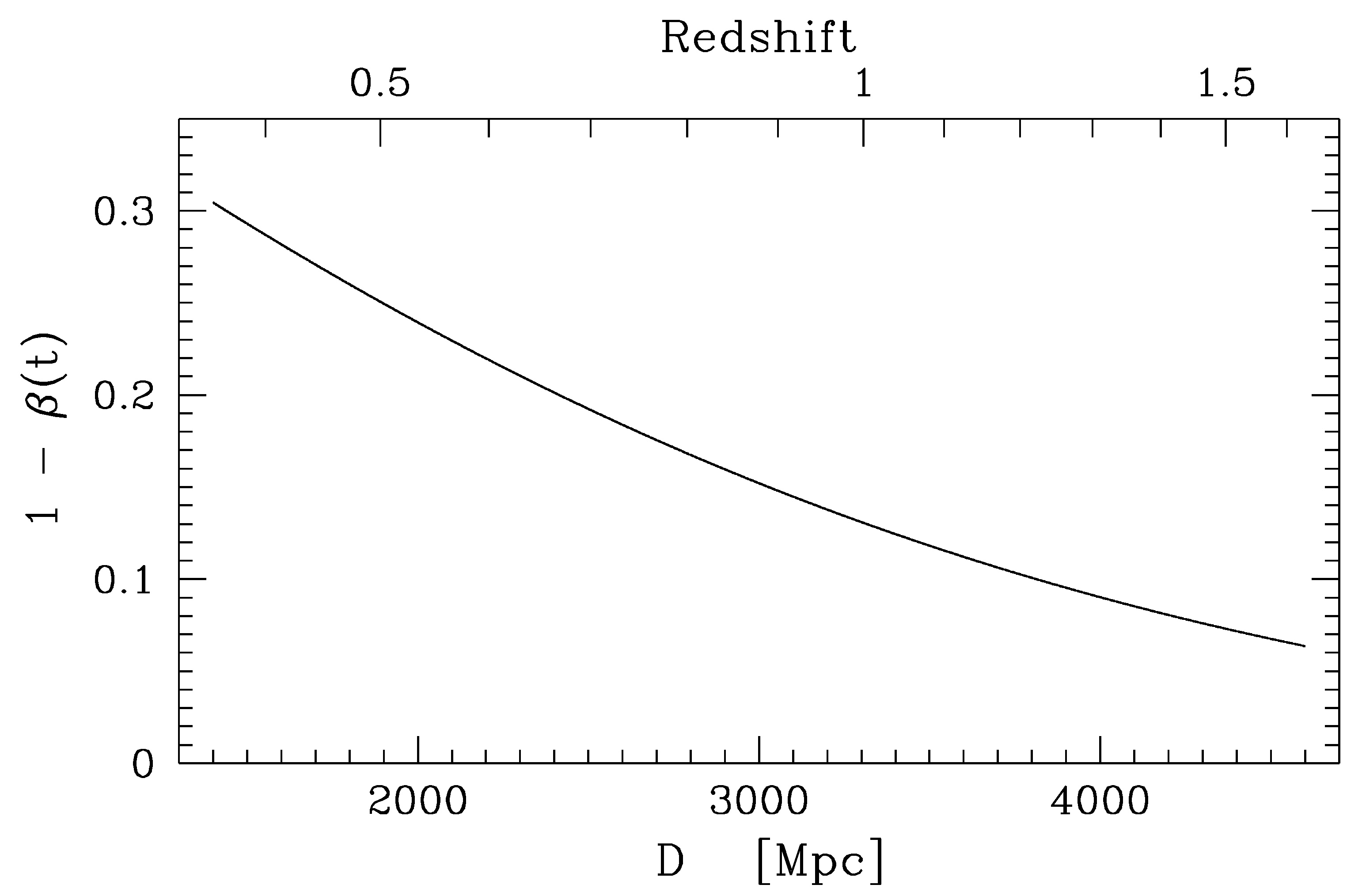
Figure 10: Variations of the $1-\beta$ parameter that define magnitude of the ISW effect (Eq. 7) for $\Omega_{\Lambda}=0.70$ and $\Omega_{\rm m}=0.3$.

In the paper we examine the correlation between the CMB temperature and the entire quasar population disregarding any particular configurations of objects, while a large number of the ISW effect investigations concentrate on distinct, well-defined galaxy structures, supervoids or superclusters, and their imprint on the CMB map. Thus, our results and several recent investigations are not directly comparable, and the objective of this discussion is limited to qualitative assessments to what extent the present estimates of the ISW amplitude are consistent with other reports. Nevertheless, such observation is still instructive because of the persistent controversy surrounding the positive detection of the ISW signal at a level of several $\mu$K.

The present statistics provides only the lower limit for the signal, but it is free from biases introduced by various void/cluster finding algorithms, and it is essentially free from the systematic errors introduced by simulations. Although our method is based on the simplified relationship between gravitational potential and the density distribution, it yields restrictive constraints on the ISW effect. Apparently, our limits at a level of several $\mu$K favour high estimates of the ISW signal, comparable to those found by Nadathur & Crittenden (2016) and exceed the best estimates predicted for the $\Lambda$CDM cosmology (see their Fig. 3).

Potentially informative is comparison of the present results with the ISW model maps obtained by Watson et al. (2014) based on Jubilee simulations. In their Fig. 7 $1\sigma$ temperature fluctuations expected in the standard $\Lambda$CDM cosmology are shown separately for a number of redshift shells of fixed width $\Delta z=0.1$. In five such shells matching our near sample $1500-3000$ Mpc ($0.38<z<0.88$), predicted $1\sigma$ fluctuations drop from $\sim 3\,\mu$K for the nearest bin to $\lesssim 2\,\mu$K for the farthest one. The joint effect of all five shells depends strongly on the correlations between the shells. For the perfect correlation the total fluctuation amplitude generated between $1500$ and $3000$ Mpc would approach our best estimate of $\sigma_{\rm o}$ at $11-12\,\mu$K (see Watson’s et al. Fig. 7). Visual inspection of maps in Watson et al. (2014) Fig. 6 shows that the ISW signal is in fact strongly correlated over the examined redshift range, and the expected $1\sigma$ fluctuations are comparable to our $\sigma_{\rm o}$.

Statistical significance of our $\sigma_{\rm o}$ measurements in the distant bin $3000-4500$ Mpc ($0.88<z<1.57$) is low (Fig. 8). However, positive $\delta T-\Delta Q$ correlations over a wide range of the test $r_{\rm s}$ values indicate a likely detection of the ISW effect also in this bin. The best estimates of $\sigma_{\rm o}$ reach $\sim 8\,\mu$K, and the Watson et al. (2014) signal has comparable amplitude assuming significant correlations of fluctuations in the contributing redshift shells.

Apparent coincidences between the Watson et al. (2014) amplitudes and our $\sigma_{\rm o}$ estimates is puzzling because both results represent different quantities. The total rms fluctuations predicted from the simulations correspond to our $\sigma_{\rm s}$ in Eq. 19, and not to $\sigma_{\rm o}$ alone. Clearly, our statistics based on quasar counts along the line of sight is unable to reconstruct variations of the gravitational potential in a way it is done by the present day cosmological simulations. Nevertheless, this statistics provides constraining limit on the ISW effect. To examine if in fact the observed signal is reproduced in the $\Lambda$CDM cosmological simulations, one should use the simulations to generate the model ISW imprint in the CMB maps, and to create quasar distribution analogous to the SDSS catalogue. Then, one should apply the $\Delta Q$ statistics to the mock quasar data to obtain constraints on the ISW effect. Eventually the comparison of these constraints with the model ISW would allow us to answer if the observed ISW signal is compatible with the $\Lambda$CDM cosmology.

Possible origins for the observed amplitude of the ISW effect are discussed by Cai et al. (2017), who investigated both lensing and temperature signatures of voids on the CMB. Using the DR12 SDSS CMASS galaxy sample they confirm reports that the temperature variations associated with large voids is substantially stronger than those predicted for the $\Lambda$CDM model, but ’the amplitude of the lensing convergence signal $\Delta\kappa$ is a very good match to $\Lambda$CDM’. Cai et al. (2017) indicate that both observables ‘may provide valuable information on cosmology and gravity’.

Stronger than expected correlation of the CMB temperature with the matter density fluctuations could indicate some departures from the standard $\Lambda$CDM model. This point was raised by Nadathur et al. (2012) and Kovács et al. (2017). In particular, such inconsistency could imply some dark matter - dark energy interactions (Olivares et al., 2008). However, it is possible that the observed correlation cannot be attributed solely to the ISW effect, i.e. some fraction of the signal is produced in a different mechanism. To support this conjecture, we note that a positive correlation between the temperature amplitude and quasar (or galaxy) concentration independent from the ISW effect should also be considered. Exact contribution of numerous classes of foreground objects at microwave frequencies is difficult to assess. Simple interpolation of the ‘spectrum of the Universe’ (Hill et al., 2018) between two spectral domains adjacent to the CMB maximum, i.e. radio below $\sim 3\cdot 10^{8}$ Hz and far infra red above $\sim 10^{12}$ Hz, gives in the microwave range flux exceeding $0.001$ of the relic CMB. This figure surpasses the potential ISW signal by more than two orders of magnitude.

Despite a ‘tremendous effort’ (Kovács et al., 2017) put to eliminate foreground emission, it is possible that some residual contamination of the relic radiation by sources with spectral energy distribution resembling the CMB cannot be ruled out. Such sources would not be removed in the Planck data processing aimed to cut-off the foreground emission. Also, their imprint on the CMB would not violate the Planck Collaboration XIX (2014) conclusion that the signal correlated with the large scale structures is achromatic over a Planck spectral range. Thus, even minute contribution of those hypothetical sources could remove the discrepancy. One should note, that both average galaxy spectrum and spectra of various AGN types differ significantly from the CMB spectrum. Nevertheless, if a small population of those specific sources exists, a precise calibration of the ISW effects and still more accurate assessment of all the cosmic background components are needed before potential deviations from the standard $\Lambda$CDM cosmology are contemplated.

Appendix A Linear correlation statistics

Here we derive basic relationships between the interesting observables under the assumption that relevant quantities are linearly correlated. This concerns in particular the fluctuations of the CMB temperature, $\delta T$ and the parameter derived from the quasar space distribution, $\Delta Q$ in Sec. 4.

In the subsequent derivation $t$ and $q$ denote single measurements of $\delta T$ and $\Delta Q$, respectively. The observed amplitude $t=s+b$, where $s$ is the temperature fluctuation of the ISW effect generated by the potential distribution within the considered distance range, $D_{\rm l}$ and $D_{\rm h}$, and $b$ represents the total ‘background’ fluctuations uncorrelated with the matter distribution in this area. It is assumed that $b$ and $s$ are uncorrelated, and the expected values of both variables are equal to zero, $\mu_{\rm b}=0$ and $\mu_{\rm s}=0$. No other specific constraints are imposed on the distributions of both variables. In particular, the dispersions $\sigma_{\rm b}$ and $\sigma_{\rm s}$ are unknown, and satisfy usual relationship $\sigma_{\rm b}^{2}\,+\,\sigma_{\rm s}^{2}\,=\,\sigma_{\rm t}^{2}$, where $\sigma_{\rm t}$ denote the observed rms scatter of $t$.

The variable $q$ by its very nature is correlated with the matter density along the line of sight. The expected value of the variable, $\mu_{\rm q}=0$. It is also subject to random fluctuations caused by a discrete nature of quasar data. Consequently, it is assumed that $q$ is adequately represented by a sum of two components: $q\,=\,c\,+\,r$, where $c$ represents quasar ‘clustering’, i.e. the component actually correlated with the ISW signal, and $r$ describes random fluctuations produced by Poisson noise.

In Sec. 4 statistical characteristics of the $q$ and $t$ distributions are discussed. Their variances, $\sigma_{\rm t}^{2}$ and $\sigma_{\rm q}^{2}$, are determined. It is shown that variables $q$ and $t$ are linearly correlated The interesting parameters of the distribution of the $r$ component, i.e. the expected value and variance, $\mu_{\rm r}$ and $\sigma_{\rm r}^{2}$ were determined using the Monte Carlo simulations for all the combinations of sphere radii and distance bins. In the whole range of sphere radii considered in the paper the random scatter of $q$ resulting from discrete quasar distribution constitutes a dominating fraction of $\sigma_{\rm q}$. Consequently, the dispersion of $c$ is small as compared to $\sigma_{\rm r}$, and it is legitimate to assume that the $c$ and $r$ are uncorrelated, and to put $\sigma_{\rm q}^{2}\,=\,\sigma_{\rm c}^{2}\,+\,\sigma_{\rm r}^{2}$.

Variables $s$ and $c$ are not directly observable. However, amplitude of their intrinsic correlation generates the correlation between $t$ and $q$ that is determined from the data. Therefore, the amplitude of the $q-t$ correlation allows to estimate some interesting parameters of the joint distribution of variables $s$ and $c$. Similarly to the pair of variables $(s,\,c)$, the pair $(s,\,q)$ is linearly correlated with the relevant parameters: $\mu_{s}\,=\,0$, $\mu_{q}\,=\,0$, $\sigma_{\rm s}$, $\sigma_{\rm q}$, and $\rho_{sq}$, where only $\sigma_{\rm q}$ is directly determinable from the data.

By means of elementary calculations one gets:

$$\rho_{sq}\,=\,\rho_{sc}\,\frac{\sigma_{\rm c}}{\sigma_{\rm q}}\,,$$ (14)

$$\rho_{sq}\,=\,\beta_{s|q}\,\frac{\sigma_{\rm q}}{\sigma_{\rm s}}\,,\hskip 42.67912pt\rho_{sc}\,=\,\beta_{s|c}\,\frac{\sigma_{\rm c}}{\sigma_{\rm s}}\,,$$ (15)

where $\beta_{s|q}$ and $\beta_{s|c}$ are slopes of the least squares regression lines of $s$ on $q$ and $s$ on $c$, respectively. Combining Eqs. 14 and 15:

$$\frac{\beta_{s|c}}{\beta_{s|q}}\,=\,\frac{\sigma_{\rm q}^{2}}{\sigma_{\rm c}^{2}}\,.$$ (16)

The variance of $s$, $\sigma_{\rm s}^{2}$, may be decomposed into:

$$\sigma_{\rm s}^{2}\,=\,\sigma_{s|c}^{2}\,+\,\beta_{s|c}^{2}\,\sigma_{\rm c}^{2}\,,$$ (17)

where $\sigma_{s|c}$ is the rms scatter of $s$ around the regression line of $s$ on $c$. Since $\beta_{s|q}\,=\,\beta_{t|q}$ and $\sigma_{\rm c}^{2}\,=\,\sigma_{\rm q}^{2}\,-\,\sigma_{\rm r}^{2}$ :

$$\sigma_{\rm s}^{2}\,=\,\sigma_{s|c}^{2}\,+\,\beta_{t|q}^{2}\,\frac{\sigma_{\rm q}^{4}}{\sigma_{\rm q}^{2}\,-\,\sigma_{\rm r}^{2}}\,,$$ (18)

or

$$\sigma_{\rm s}^{2}\,=\,\sigma_{s|c}^{2}\,+\,\sigma_{\rm o}^{2}\,,$$ (19)

where

$$\sigma_{\rm o}\,=\,\rho_{\rm tq}\,\frac{\sigma_{\rm t}\,\sigma_{\rm q}}{\sqrt{\sigma_{\rm q}^{2}\,-\,\sigma_{\rm r}^{2}}}\,,$$ (20)

and we put $\beta_{t|q}\,=\,\rho_{\rm tq}\,\frac{\sigma_{\rm t}}{\sigma_{\rm q}}$.

In statistics the second term in the right-hand side of Eq. 19, $\sigma_{\rm o}^{2}$, represents the ‘explained’ or ‘model’ fraction of the total variance, $\sigma_{\rm s}^{2}$, while the first term remains ‘unexplained’ by the model. In the present investigation, fluctuations of the gravitational potential that generate the ISW effect are represented by the $\Delta Q$ parameter (Sec. 4). A question how accurate is this approximation is not addressed in the paper. Therefore, amplitude of the ‘unexplained’ variance $\sigma_{s|c}^{2}$ remains undetermined.

References

- Adelman-McCarthy et al. (2008) Adelman-McCarthy J. K., Agüeros M. A., Allam S. S., Allende Prieto C., Anderson K. S. J., Anderson S. F., Annis J., Bahcall N. A., Bailer-Jones C. A. L., Zucker D. B., 2008, ApJS, 175, 297
- Alam et al. (2015) Alam S., Albareti F. D., Allende Prieto C., Anders F., Anderson S. F., Anderton T., Andrews B. H., Armengaud E., Aubourg É., Bailey S., et al. 2015, ApJS, 219, 12
- Bennett et al. (2003) Bennett C. L., Bay M., Halpern M., Hinshaw G., Jackson C. e. a., 2003, ApJ, 583, 1
- Bennett et al. (2013) Bennett C. L., Larson D., Weiland J. L., Jarosik N., Hinshaw G., Odegard N., Smith K. M., Hill R. S., 2013, ApJS, 208, 20
- Cai et al. (2017) Cai Y.-C., Neyrinck M., Mao Q., Peacock J. A., Szapudi I., Berlind A. A., 2017, MNRAS, 466, 3364
- Condon et al. (1998) Condon J. J., Cotton W. D., Greisen E. W., Yin Q. F., Perley R. A., Taylor G. B., Broderick J. J., 1998, AJ, 115, 1693
- Dark Energy Survey Collaboration (2016) Dark Energy Survey Collaboration 2016, MNRAS, 460, 1270
- Dodelson (2003) Dodelson S., 2003, Modern cosmology. Academic Press
- Flaugher et al. (2015) Flaugher B., Diehl H. T., Honscheid K., Abbott T. M. C., Alvarez O. e. a., 2015, AJ, 150, 150
- Giannantonio et al. (2012) Giannantonio T., Crittenden R., Nichol R., Ross A. J., 2012, MNRAS, 426, 2581
- Górski et al. (2005) Górski K. M., Hivon E., Banday A. J., Wandelt B. D., Hansen F. K., Reinecke M., Bartelmann M., 2005, ApJ, 622, 759
- Granett et al. (2015) Granett B. R., Kovács A., Hawken A. J., 2015, MNRAS, 454, 2804
- Granett et al. (2008) Granett B. R., Neyrinck M. C., Szapudi I., 2008, ApJ, 683, L99
- Granett et al. (2009) Granett B. R., Neyrinck M. C., Szapudi I., 2009, ApJ, 701, 414