Convergence Rates of First and Higher Order Dynamics for Solving Linear Ill-posed Problems

Abstract

Recently, there has been a great interest in analysing dynamical flows, where the stationary limit is the minimiser of a convex energy. Particular flows of great interest have been continuous limits of Nesterov’s algorithm and the Fast Iterative Shrinkage-Thresholding Algorithm (FISTA), respectively.

In this paper we approach the solutions of linear ill-posed problems by dynamical flows. Because the squared norm of the residual of a linear operator equation is a convex functional, the theoretical results from convex analysis for energy minimising flows are applicable. However, in the restricted situation of this paper they can often be significantly improved. Moreover, since we show that the proposed flows for minimising the norm of the residual of a linear operator equation are optimal regularisation methods and that they provide optimal convergence rates for the regularised solutions, the given rates can be considered the benchmarks for further studies in convex analysis.
Keywords: Linear ill-posed problems, regularisation theory, dynamical regularisation, optimal convergence rates, Showalter’s method, heavy ball method, vanishing viscosity flow, spectral analysis

²Institute for Mathematics
Humboldt University of Berlin
Unter den Linden 6
10099 Berlin, Germany

³Weierstrass Institute for Applied
   Analysis and Stochastics (WIAS)
Mohrenstraße 39
10117 Berlin, Germany

⁴Johann Radon Institute for Computational
   and Applied Mathematics (RICAM)
Altenbergerstraße 69
A-4040 Linz, Austria

MSC 2010: 47A52, 47N10, 65J20

1. Introduction

We consider the problem of solving a linear operator equation

$$Lx=y,$$ (1.1)

where $L\colon\mathcal{X}\rightarrow\mathcal{Y}$ is a bounded linear operator between (infinite dimensional) real Hilbert spaces $\mathcal{X}$ and $\mathcal{Y}$. If the range of $L$ is not closed, Equation 1.1 is ill-posed, see [13], in the sense that small perturbations in the data $y$ can cause non-solvability of the Equation 1.1 or large perturbations of the corresponding solution of Equation 1.1 by perturbed right hand side. These undesirable effects are prevented by regularisation.

In this particular paper we consider dynamical regularisation methods for solving Equation 1.1. That is, we approximate the minimum norm solution $x^{\dagger}$ of Equation 1.1 by the solution $\xi$ of a dynamical system of the form

$$\xi^{(N)}(t)+\sum_{k=1}^{N-1}a_{k}(t)\xi^{(k)}(t) =-L^{*}L\xi(t)+L^{*}\tilde{y} \text{for all }t\in\left(0,\infty\right),$$ (1.2)

$$\xi^{(k)}(0) =0 \text{for all }k=0,\ldots,N-1,$$

at an appropriate time, where $N\in\mathds{N}$, $a_{k}\colon(0,\infty)\to\mathds{R}$, $k=1,\ldots,N-1$, are continuous functions, and $\tilde{y}$ is a perturbation of $y$. The stopping time is in practice often chosen via a standard discrepancy principle, see [13, Chapter 3.3]. We are now interested under which conditions the regularised solution $\xi(t)$ can be guaranteed to converge to the solution $x^{\dagger}$ as $t\to\infty$ and how fast this convergence happens.

Studying first the case of exact data $\tilde{y}=y$, it turns out that the convergence rate, that is, the decay of $\|\xi(t)-x^{\dagger}\|^{2}$ in the limit $t\to\infty$, can be uniquely characterised by the spectral decomposition of the minimum norm solution $x^{\dagger}$ with respect to the operator $L^{*}L$, which allows us to get optimal convergence rates as a function of the “regularity” of the source $x^{\dagger}$. This regularity is usually described by so-called source conditions, the most common ones being of the form $x^{\dagger}\in\mathcal{R}((L^{*}L)^{\frac{\mu}{2}})$ for some $\mu>0$; we refer to [13, Chapter 2.2] and [9, Chapter 3.2] for an introduction to the use of those source conditions for obtaining convergence rates. Moreover, these convergence rates for exact data are seen to be in a one-to-one correspondence to certain convergence rates for perturbed data as the perturbation $\|\tilde{y}-y\|^{2}$ goes to zero.

Outside the regularisation community source conditions might appear technical because they involve the operator $L$. However, it was demonstrated that for differential and integral operators $L$, these conditions very well coincide with smoothness conditions in Sobolev spaces. See for instance [14], where the analogy of smoothness and source conditions has been explained for the problem of numerical differentiation. For this analogy these conditions are also often termed smoothness conditions.

In particular, we will apply the general theory of this equivalent characterisation of convergence rates to the following three, well-studied examples:

1. Showalter’s method (also known as the gradient flow method), see [27, 28], which corresponds to the case $N=1$ in Equation 1.2:

   $$\xi^{\prime}(t) =-L^{*}L\xi(t)+L^{*}\tilde{y}\text{ for all }t\in\left(0,\infty\right),$$ (1.3)

   $$\xi(0) =0,$$

   see Table 1 for an overview of the available convergence rates results;

2. the heavy ball method, introduced in [22], corresponding to $N=2$ with a constant function $a_{1}(t)=b>0$ in Equation 1.2:

   $$\partial_{tt}\xi(t;\tilde{y})+b\partial_{t}\xi(t;\tilde{y}) =-L^{*}L\xi(t;\tilde{y})+L^{*}\tilde{y}\text{ for all }t\in\left(0,\infty\right),$$

   $$\partial_{t}\xi(0;\tilde{y}) =0,$$ (1.4)

   $$\xi(0;\tilde{y}) =0,$$

   where known convergence rates results are collected in Table 2;

3. the vanishing viscosity method, see [29], which is the case of $N=2$ with $a_{1}(t)=\frac{b}{t}$ for some $b>0$ in Equation 1.2:

   $$\partial_{tt}\xi(t;\tilde{y})+\frac{b}{t}\partial_{t}\xi(t;\tilde{y}) =-L^{*}L\xi(t;\tilde{y})+L^{*}\tilde{y}\text{ for all }t\in\left(0,\infty\right),$$

   $$\partial_{t}\xi(0;\tilde{y}) =0,$$ (1.5)

   $$\xi(0;\tilde{y}) =0.$$

   Some convergence rates from the literature are listed in Table 3.

Source Condition	$\left\|\xi(t)-x^{\dagger}\right\|^{2}$		$\left\|L\xi(t)-y\right\|^{2}$
$\|L^{\dagger}\|<\infty$	$\mathcal{O}(\mathrm{e}^{-\|L^{\dagger}\|^{-2}t})$	[27, Theorem 1]	$\mathcal{O}(\mathrm{e}^{-\|L^{\dagger}\|^{-2}t})$
$x^{\dagger}\in\mathcal{R}((L^{*}L)^{\frac{\mu}{2}})$	$\mathcal{O}(t^{-\mu})$	[28, Theorem 1] ($\mu=1$), Section 4	$\mathcal{O}(t^{-\mu-1})$	Section 4
$x^{\dagger}\in\mathcal{N}(L)^{\perp}$	$o(1)$	[28, Theorem 1], Section 4 with Section 2.1	$\mathcal{O}(t^{-1})$ $o(t^{-1})$	[28, Theorem 1] Section 4 with Section 2.6

Table 1: Convergence rates for Showalter’s method. (To compare the results from [28], we remark that the condition $y\in\mathcal{R}(LL^{*})$ given therein is equivalent to $x^{\dagger}\in\mathcal{R}((L^{*}L)^{\frac{1}{2}})$, which can be directly seen, for example, from the characterisation of the range of a dual operator given in [26, Lemma 8.31].)
We also remark that in the well-posed case $\|L^{\dagger}\|<\infty$, the rates for $\|\xi(t)-x^{\dagger}\|^{2}$ and for $\|L\xi(t)-y\|^{2}$ are always the same, since $\|L^{\dagger}\|^{-2}\|\xi(t)-x^{\dagger}\|^{2}\leq\|L\xi(t)-y\|^{2}\leq\|L\|^{2}\|\xi(t)-x^{\dagger}\|^{2}$.

Source Condition	$\left\|\xi(t)-x^{\dagger}\right\|^{2}$		$\left\|L\xi(t)-y\right\|^{2}$
$\|L^{\dagger}\|<\infty$	$\mathcal{O}(\mathrm{e}^{\varepsilon t-\beta(\|L^{\dagger}\|)\frac{bt}{2}})$	[22, Theorem 9.(5)]	$\mathcal{O}(\mathrm{e}^{\varepsilon t-\beta(\|L^{\dagger}\|)\frac{bt}{2}})$
$x^{\dagger}\in\mathcal{R}((L^{*}L)^{\frac{\mu}{2}})$	$\mathcal{O}(t^{-\mu})$	[33, Theorem 5.1], Section 5	$\mathcal{O}(t^{-\mu-1})$	Section 5
$x^{\dagger}\in\mathcal{N}(L)^{\perp}$	$o(1)$	Section 5 with Lemma 5.7 and Section 2.1	$o(t^{-1})$	[33, Lemma 3.2] ($b\geq\|L\|$), Section 5 with Lemma 5.7 and Section 2.6

Table 2: Convergence rates for the heavy ball method. Here, $\varepsilon>0$ denotes an arbitrarily small parameter and we have set $\beta(\|L^{\dagger}\|)=1-(1-\frac{4}{b^{2}\|L^{\dagger}\|^{2}})^{\frac{1}{2}}$ for $\|L^{\dagger}\|\geq\frac{2}{b}$ and $\beta(\|L^{\dagger}\|)=1$ for $\|L^{\dagger}\|<\frac{2}{b}$.

Source Condition	Parameters	$\left\|\xi(t)-x^{\dagger}\right\|^{2}$		$\left\|L\xi(t)-y\right\|^{2}$
$\|L^{\dagger}\|<\infty$	$b>3$	$o(t^{-2})$		$o(t^{-2})$	[4, Theorem 4.16]
		$\mathcal{O}(t^{-\frac{2b}{3}})$	[5, Theorem 3.4]	$\mathcal{O}(t^{-\frac{2b}{3}})$	[5, Theorem 3.4]
$\|L^{\dagger}\|<\infty$	$b>2$	$\mathcal{O}(t^{-2})$		$\mathcal{O}(t^{-2})$	[29, Theorem 7]
		$\mathcal{O}(t^{-b})$		$\mathcal{O}(t^{-b})$	[7, Theorem 4.2]
$\|L^{\dagger}\|<\infty$	$0<b<3$	$\mathcal{O}(t^{-\frac{2b}{3}})$		$\mathcal{O}(t^{-\frac{2b}{3}})$	[4, Theorem 4.19]
$x^{\dagger}\in\mathcal{R}((L^{*}L)^{\frac{\mu}{2}})$	$0<\mu<\frac{b}{2}$	$\mathcal{O}(t^{-2\mu})$	Section 6
$x^{\dagger}\in\mathcal{R}((L^{*}L)^{\frac{\mu}{2}})$	$0<\mu<\frac{b}{2}-1$			$\mathcal{O}(t^{-2\mu-2})$	Section 6
$x^{\dagger}\in\mathcal{N}(L)^{\perp}$	$b\geq 3$			$\mathcal{O}(t^{-2})$	[5, Theorem 2.7]
$x^{\dagger}\in\mathcal{N}(L)^{\perp}$	$b>0$	$o(1)$	Section 6 with Lemma 6.5 and Section 2.1	$\mathcal{O}(t^{-b+\varepsilon})+o(t^{-2})$	Section 6 with Lemma 6.5 and Section 2.6 and Section 2.6

Table 3: Convergence rates for the vanishing viscosity flow. As before, $\varepsilon>0$ denotes an arbitrarily small parameter.

Especially the vanishing viscosity method has recently been heavily investigated, see [29, 8, 5, 6], for example, as it shows a faster convergence compared to the other two methods, and it was demonstrated to be a time continuous formulation of Nesterov’s algorithm, see [20], providing an explanation of the rapid convergence of this algorithm. Consequently, it was not only studied in the form of Equation 1.5, but more generally with the right hand side (which in Equation 1.5 is the negative gradient of $\mathcal{J}_{0}(x)=\frac{1}{2}\|Lx-y\|^{2}$) replaced by the negative gradient of an arbitrary convex and differentiable functional $\mathcal{J}$. But, since our theory relies on spectral analysis, we limit our discussion to the quadratic functional $\mathcal{J}_{0}$.

In terms of convergence rates, however, the discussions for general functionals $\mathcal{J}$ are often limited to the estimation of the convergence of $\mathcal{J}(\xi(t))-\min_{x\in\mathcal{X}}\mathcal{J}(x)$, which for $\mathcal{J}=\mathcal{J}_{0}$ is given by $\frac{1}{2}\|L\xi(t)-y\|^{2}$. In the well-posed case where the operator $L$ has a bounded pseudoinverse $L^{\dagger}$, this convergence of the squared norm of the residual is equivalent to the convergence of the error $\|\xi(t)-x^{\dagger}\|^{2}$, but this is no longer true in the ill-posed case where the pseudoinverse is unbounded. In contrast to this, our approach directly gives convergence rates for $\|\xi(t)-x^{\dagger}\|^{2}$, which then imply a convergence (typically of higher order) of the squared norm of the residual.

We will proceed as follows:

• In Section 2 we revisit convergence rates results of regularisation methods from [3], which, in particular, allow to analyse first and higher order dynamics.

• In the following sections we apply the general results of Section 2 to regularising flow equations. In Section 4 we derive well-known convergence rates results of Showalter’s method and prove optimality of this method. In Section 5 we prove regularising properties, optimality and convergence rates of the heavy ball dynamical flow. In the context of inverse problems this method has already been analysed by [33], however not in terms of optimality, as it is done here.

• In Section 6 we consider the vanishing viscosity flow. We apply the general theory of Section 2 and prove optimality of this method. In particular we prove under source conditions (see for instance [13, 9]) optimal convergence rates (in the sense of regularisation theory) for $\|\xi(t)-x^{\dagger}\|^{2}$. These rates (and the resulting ones for the squared norm of the residual) are seen to interpolate nicely between the known rates in the well-posed (finite-dimensional) and those in the ill-posed setting when varying the regularity of the solution $x^{\dagger}$ (via changing the parameter $\mu$ in Table 3).

We want to emphasise that the terminologies optimal from [7] (a representative reference for this field) and [3] differ by the class of problems and the amount of a priori information taken into account. In [7] best worst case error rates in the class of convex energies are derived, while we focus on squared functionals $\mathcal{J}$. Moreover, we take into account prior knowledge on the solution. In view of this, it is not surprising that we get different “optimal” rates.

2. Generalisations of Convergence Rates Results

In the following we slightly generalise convergence rates and saturation results from [3] so that they can be applied to prove convergence of the second order regularising flows in Section 5 and Section 6. Thereby one needs to be aware that in classical regularisation theory, the regularisation parameter $\alpha>0$ is considered a small parameter, meaning that we consider small perturbations of Equation 1.1. For dynamic regularisation methods of the form of Equation 1.2 we take large times to approximate the stationary state. To link these two theories, we will apply an inverse polynomial identification of optimal regularisation time and regularisation parameter.

Let $L\colon\mathcal{X}\to\mathcal{Y}$ be a bounded linear operator between two real Hilbert spaces $\mathcal{X}$ and $\mathcal{Y}$ with operator norm $\left\|L\right\|$, $y\in\mathcal{R}(L)$, and let $x^{\dagger}\in\mathcal{X}$ be the minimum norm solution of $Lx=y$ defined by

$$Lx^{\dagger}=y\text{ and }\|x^{\dagger}\|=\inf\{\left\|x\right\|\mid Lx=y\}.$$

Definition .

We call a family $(r_{\alpha})_{\alpha>0}$ of continuous functions $r_{\alpha}\colon[0,\infty)\to[0,\infty)$ the generator of a regularisation method if

1. there exists a constant $\sigma\in(0,1)$ such that

   $$r_{\alpha}(\lambda)\leq\min\left\{\frac{2}{\lambda},\frac{\sigma}{\sqrt{\alpha\lambda}}\right\}\text{ for every }\lambda>0,\;\alpha>0;$$ (2.1)

2. the error function $\tilde{r}_{\alpha}\colon(0,\infty)\to[-1,1]$, defined by

   $$\tilde{r}_{\alpha}(\lambda)=1-\lambda r_{\alpha}(\lambda),\;\lambda>0,$$ (2.2)

   is non-negative and monotonically decreasing on the interval $(0,\alpha)$;

3. there exists for every $\alpha>0$ a monotonically decreasing, continuous function $\tilde{R}_{\alpha}\colon(0,\infty)\to\left[0,1\right]$ such that

   $$\tilde{R}_{\alpha}\geq|\tilde{r}_{\alpha}|\text{ and }\alpha\mapsto\tilde{R}_{\alpha}(\lambda)\text{ is continuous and monotonically increasing for every fixed }\lambda>0;$$

4. there exists for every $\bar{\alpha}>0$ a constant $\tilde{\sigma}\in(0,1)$ such that

   $$\tilde{R}_{\alpha}(\alpha)<\tilde{\sigma}\text{ for all }\alpha\in(0,\bar{\alpha}).$$

Remark:

The definition of the generator of a regularisation method differs from the one in [3] by allowing the regularisation method to overshoot, meaning that $r_{\alpha}(\lambda)>\frac{1}{\lambda}$ is possible at some points $\lambda>0$ (the choice $r_{\alpha}(\lambda)=\frac{1}{\lambda}$, which is not a regularisation method in the sense of Section 2, would correspond to taking the inverse without regularisation, see Equation 2.3). Consequently, we also relaxed the assumption that the error function $\tilde{r}_{\alpha}$ is monotonically decreasing to the existence of a monotonically decreasing upper bound $\tilde{R}_{\alpha}$ for $\tilde{r}_{\alpha}$. We also want to remark that in the definition of the error function in [3], $\tilde{r}_{\alpha}^{\text{\cite[cite]{[\@@bibref{}{AlbElbHooSch16}{}{}]}}}$, there is an additional square included, that is, $\tilde{r}_{\alpha}^{\text{\cite[cite]{[\@@bibref{}{AlbElbHooSch16}{}{}]}}}=\tilde{r}_{\alpha}^{2}$.

Definition .

Let $(r_{\alpha})_{\alpha>0}$ be the generator of a regularisation method.

1. The regularised solutions according to a generator $(r_{\alpha})_{\alpha>0}$ and data $\tilde{y}$ are defined by

   $$x_{\alpha}\colon\mathcal{Y}\to\mathcal{X},\;x_{\alpha}(\tilde{y})=r_{\alpha}(L^{*}L)L^{*}\tilde{y},$$ (2.3)

   where we use the bounded Borel functional calculus to identify the function $r_{\alpha}\colon[0,\infty)\to[0,\infty)$ with a function acting on the space of positive semi-definite self-adjoint operators, see [32, Chapter XI.12], for example.

2. Let $(\tilde{R}_{\alpha})_{\alpha>0}$ be as in Section 2 (iii). Then we define for all $\alpha>0$ the envelopes

   $$R_{\alpha}\colon(0,\infty)\to[0,\infty),\;R_{\alpha}(\lambda)=\frac{1}{\lambda}\left(1-\tilde{R}_{\alpha}(\lambda)\right),$$ (2.4)

   and the corresponding regularised solutions

   $$X_{\alpha}\colon\mathcal{Y}\to\mathcal{X},\;X_{\alpha}(\tilde{y})=R_{\alpha}(L^{*}L)L^{*}\tilde{y}.$$ (2.5)

Remark:

The family $(R_{\alpha})_{\alpha>0}$ is also a generator of a regularisation method, since we have

$$R_{\alpha}(\lambda)=\frac{1-\tilde{R}_{\alpha}(\lambda)}{\lambda}\leq\frac{1-\tilde{r}_{\alpha}(\lambda)}{\lambda}=r_{\alpha}(\lambda)\leq\min\left\{\frac{2}{\lambda},\frac{\sigma}{\sqrt{\alpha\lambda}}\right\}\text{ for every }\lambda>0,\;\alpha>0,$$ (2.6)

which verifies Section 2 (i); and the other three conditions of Section 2 are tautologically fulfilled: Section 2 (ii) by the definition of $\tilde{R}_{\alpha}$ via Section 2 (iii), and Section 2 (iii) and (iv) by choosing $\tilde{R}_{\alpha}$ itself as upper bound for $|\tilde{R}_{\alpha}|$.

The idea of these regularised solutions is to replace the unbounded inverse of $L\colon\mathcal{N}(L)^{\perp}\to\mathcal{R}(L)$ by the bounded approximation $x_{\alpha}$, where the parameter $\alpha>0$ quantifies the regularisation. It should disappear in the limit $\alpha\to 0$, where we typically expect $r_{\alpha}(\lambda)\to\frac{1}{\lambda}$ corresponding to $x_{\alpha}(y)\to(L^{*}L)^{\dagger}L^{*}y=x^{\dagger}$ (this is, however, not enforced by Section 2, but we will add in Section 2.2 a compatibility condition to ensure this).

Example .

The most prominent regularisation method is probably Tikhonov regularisation, where the regularised solution $x_{\alpha}(\tilde{y})$ is defined as the minimisation point of the Tikhonov functional

$$\mathcal{T}_{\alpha,\tilde{y}}\colon\mathcal{X}\to\mathds{R},\;\mathcal{T}_{\alpha,\tilde{y}}(x)=\|Lx-\tilde{y}\|^{2}+\alpha\|x\|^{2}.$$

Solving the optimality condition, gives us for $x_{\alpha}(\tilde{y})$ the expression

$$x_{\alpha}(\tilde{y})=(L^{*}L+\alpha I)^{-1}L^{*}\tilde{y},$$

where $I\colon\mathcal{X}\to\mathcal{X}$ denotes the identity map on $\mathcal{X}$, which has with $r_{\alpha}(\lambda)\coloneqq\frac{1}{\lambda+\alpha}$ the form of Equation 2.3 and $r_{\alpha}$ satisfies all the conditions of Section 2, see [3, Example 2.4].

We will show later in Section 4, Section 5, and Section 6 that also some common dynamical regularisation methods fall into this regularisation scheme so that all the convergence rates results from this section can be applied to these methods.

Definition .

We denote by $A\mapsto\mathbf{E}_{A}$ and $A\mapsto\mathbf{F}_{A}$ the spectral measures of the operators $L^{*}L$ and $LL^{*}$, respectively, on all Borel sets $A\subseteq[0,\infty)$; and we define the right-continuous and monotonically increasing function

$$e\colon(0,\infty)\to[0,\infty),\;e(\lambda)=\|\mathbf{E}_{[0,\lambda]}x^{\dagger}\|^{2}.$$ (2.7)

We remark that the minimum norm solution $x^{\dagger}$ is in the orthogonal complement of the null space $\mathcal{N}(L)$ of $L$ and we therefore have $\mathbf{E}_{[0,\lambda]}x^{\dagger}=\mathbf{E}_{(0,\lambda]}x^{\dagger}$.

Moreover, if $f\colon(0,\infty)\to\mathds{R}$ is a right-continuous, monotonically increasing, and bounded function, we write

$$\int_{a}^{b}g(\lambda)\,\mathrm{d}f(\lambda)=\int_{(a,b]}g(\lambda)\,\mathrm{d}\mu_{f}(\lambda)$$

for the Lebesgue–Stieltjes integral of $f$, where $\mu_{f}$ denotes the unique non-negative Borel measure defined by $\mu_{f}((\lambda_{1},\lambda_{2}])=f(\lambda_{2})-f(\lambda_{1})$ and $g\in L^{1}(\mu_{f})$.

We introduce the following quantities, whose behaviour we want to relate to each other:

• the spectral tail of the minimum norm solution $x^{\dagger}$ with respect to the operator $L^{*}L$, that is, the asymptotic behaviour of $e(\lambda)$ as $\lambda$ tends to zero, see [21];

• the error between the minimum norm solution $x^{\dagger}$ and the regularised solution $x_{\alpha}(y)$ or $X_{\alpha}(y)$ for the exact data $y$ called the noise free regularisation error, that is,

  $$d(\alpha)\coloneqq\left\|x_{\alpha}(y)-x^{\dagger}\right\|^{2}\text{ and }D(\alpha)\coloneqq\left\|X_{\alpha}(y)-x^{\dagger}\right\|^{2},$$ (2.8)

  respectively, as $\alpha$ tends to zero;

• the best worst case error between the minimum norm solution $x^{\dagger}$ and the regularised solution $x_{\alpha}(\tilde{y})$ or $X_{\alpha}(\tilde{y})$ for some data $\tilde{y}$ with distance less than or equal to $\delta>0$ to the exact data $y$ under optimal choice of the regularisation parameter $\alpha$, that is,

  $$\tilde{d}(\delta)\coloneqq\sup_{\tilde{y}\in\bar{B}_{\delta}(y)}\inf_{\alpha>0}\left\|x_{\alpha}(\tilde{y})-x^{\dagger}\right\|^{2}\text{ and }\tilde{D}(\delta)\coloneqq\sup_{\tilde{y}\in\bar{B}_{\delta}(y)}\inf_{\alpha>0}\left\|X_{\alpha}(\tilde{y})-x^{\dagger}\right\|^{2},$$ (2.9)

  respectively, as $\delta$ tends to zero;

• the noise free residual error, which is the error between the image of the regularised solution $x_{\alpha}(y)$ or $X_{\alpha}(y)$ and the exact data $y$, that is,

  $$q(\alpha)\coloneqq\|Lx_{\alpha}(y)-y\|^{2}\text{ and }Q(\alpha)\coloneqq\|LX_{\alpha}(y)-y\|^{2},$$ (2.10)

  respectively, as $\alpha$ tends to zero.

To describe the behaviour of these quantities, we consider, for example, convergence rates of the form

$$d(\alpha)=\|x_{\alpha}(y)-x^{\dagger}\|^{2}\leq C_{d}\varphi(\alpha)\text{ for all }\alpha>0,$$

with some constant $C_{d}>0$ for the noise free regularisation error $d$, characterised by the decay of a monotonically increasing function $\varphi\colon(0,\infty)\to(0,\infty)$ for $\alpha\to 0$, and look for a corresponding (equivalent) characterisation of the convergence rates of the other quantities, such as $e(\lambda)=\|\mathbf{E}_{[0,\lambda]}x^{\dagger}\|^{2}$ or $q(\alpha)=\left\|Lx_{\alpha}(y)-y\right\|^{2}$.

Example .

Common families of functions $\varphi$ used to describe the convergence rates are Hölder functions

$$\varphi^{\mathrm{H}}_{\mu}\colon(0,\infty)\to\mathds{R},\;\varphi^{\mathrm{H}}_{\mu}(\alpha)=\alpha^{\mu}\text{ for all }\mu>0,$$ (2.11)

see [13], for example; and logarithmic

$$\varphi^{\mathrm{L}}_{\mu}\colon(0,\infty)\to\mathds{R},\;\varphi^{\mathrm{L}}_{\mu}(\alpha)=\begin{cases}\left|\log\alpha\right|^{-\mu},&\alpha<\mathrm{e}^{-1},\\ 1,&\alpha\geq\mathrm{e}^{-1},\end{cases}\text{ for all }\mu>0,$$ (2.12)

or even double logarithmic functions, see for instance [17, 25]. See Figure 1 for a sketch of the graphs of these functions.

Figure 1: Graphs of some common functions used to characterise convergence rates. See Section 2 for the definitions of these functions.

The main results are collected in Section 2.5 and Section 2.6. We proceed in the following way to derive them:

• In Lemma 2.1 and Section 2.1, we write the different regularisation errors in spectral form.

• In Lemma 2.2 and Lemma 2.3, we show the relations between the convergence rates of the noise free quantities $e$, $d$, and $D$. For this, we require the function $\varphi$, which describes the rate of convergence and is the same for all three quantities, to be compatible with the regularisation method, see Section 2.2.

• In Lemma 2.10 and Lemma 2.11, we derive the relations of the best worst case errors $\tilde{d}$ and $\tilde{D}$ to the quantities $e$ and $D$. The corresponding rate of convergence is hereby of the form $\Phi[\varphi]$, where the mapping $\Phi$ is introduced in Section 2.3 and some of its elementary properties are shown in Lemma 2.6, Lemma 2.7, Lemma 2.8, and Lemma 2.9.

• The statements for the residual errors $q$ and $Q$ are then concluded from Section 2.5 by using the identification of $q$ and $Q$ for the minimum norm solution $x^{\dagger}$ with the noise free errors $d$ and $D$ for the minimum norm solution $\bar{x}^{\dagger}=(L^{*}L)^{\frac{1}{2}}x^{\dagger}$ of the problem $Lx=\bar{y}$ with $\bar{y}=L\bar{x}^{\dagger}$, and they are summarised in Section 2.6, Section 2.6, and Section 2.6.

In the remaining of this section, we will always consider $(r_{\alpha})_{\alpha>0}$ to be the generator of a regularisation method with an envelope $(R_{\alpha})_{\alpha>0}$ and corresponding regularised solutions $(x_{\alpha})_{\alpha>0}$ and $(X_{\alpha})_{\alpha>0}$, respectively. Moreover, we use the functions $e$, $d$, $D$, $\tilde{d}$, $\tilde{D}$, $q$, and $Q$ as defined in Section 2, see Table 4 for a summary of the notation.

Abbreviation	Description	Reference
$r_{\alpha}$	Generator	Section 2
$R_{\alpha}$	Envelope generator	Equation 2.4
$\tilde{r}_{\alpha}$	Error function	Equation 2.2
$\tilde{R}_{\alpha}$	Envelope error function	Section 2 (iii)
$x_{\alpha}(\tilde{y})=r_{\alpha}(L^{*}L)L^{*}\tilde{y}$	Regularised solution according to $r_{\alpha}$	Equation 2.3
$X_{\alpha}(\tilde{y})=R_{\alpha}(L^{*}L)L^{*}\tilde{y}$	Regularised solution according to $R_{\alpha}$	Equation 2.5
$d(\alpha)=\left\|x_{\alpha}(y)-x^{\dagger}\right\|^{2}$	Noise free regularisation error for $r_{\alpha}$	Equation 2.8
$D(\alpha)=\left\|X_{\alpha}(y)-x^{\dagger}\right\|^{2}$	Noise free regularisation error for $R_{\alpha}$	Equation 2.8
$\tilde{d}(\delta)$	Best worst case error for $r_{\alpha}$	Equation 2.9
$\tilde{D}(\delta)$	Best worst case error for $R_{\alpha}$	Equation 2.9
$q(\alpha)=\left\|Lx_{\alpha}(y)-y\right\|^{2}$	Noise free residual error for $r_{\alpha}$	Equation 2.10
$Q(\alpha)=\left\|LX_{\alpha}(y)-y\right\|^{2}$	Noise free residual error for $R_{\alpha}$	Equation 2.10
$\mathbf{E}_{A},\mathbf{F}_{A}$	Spectral measures of $L^{*}L,LL^{*}$	Section 2
$e(\lambda)=\|\mathbf{E}_{[0,\lambda]}x^{\dagger}\|^{2}$	Spectral tail of $x^{\dagger}$	Equation 2.7
$\hat{\varphi}$	$\hat{\varphi}(\alpha)=\sqrt{\alpha\varphi(\alpha)}$	Section 2.3
$\hat{\varphi}^{-1}$	Generalised inverse of a function $\hat{\varphi}$	Section 2.3
$\Phi$	Noise-free to noisy transform	Section 2.3

Table 4: Used variables and references to their definitions.

2.1. Spectral Representations of the Regularisation Errors

To do the analysis, we will expand the quantities of interest with respect to the measure $A\mapsto\left\|\mathbf{E}_{A}x^{\dagger}\right\|^{2}$, which describes the spectral decomposition of $x^{\dagger}$ with respect to the operator $L^{*}L$. With the function $e$ defined in Equation 2.7, we can write the resulting integrals in the form of Lebesgue–Stieltjes integrals.

Lemma 2.1.

We have the representations

$$d(\alpha)=\int_{0}^{\left\|L\right\|^{2}}\tilde{r}_{\alpha}^{2}(\lambda)\,\mathrm{d}e(\lambda)\text{ and }D(\alpha)=\int_{0}^{\left\|L\right\|^{2}}\tilde{R}_{\alpha}^{2}(\lambda)\,\mathrm{d}e(\lambda)$$ (2.13)

for the regularisation errors $d$ and $D$, respectively, and

$$q(\alpha)=\int_{0}^{\left\|L\right\|^{2}}\lambda\tilde{r}_{\alpha}^{2}(\lambda)\,\mathrm{d}e(\lambda)\text{ and }Q(\alpha)=\int_{0}^{\left\|L\right\|^{2}}\lambda\tilde{R}_{\alpha}^{2}(\lambda)\,\mathrm{d}e(\lambda)$$ (2.14)

for the residuals $q$ and $Q$, respectively.

Proof:

We can write the differences between one of the regularised solutions $x_{\alpha}(y)$ or $X_{\alpha}(y)$ and the minimum norm solution $x^{\dagger}$ in the form

$$x_{\alpha}(y)-x^{\dagger} =r_{\alpha}(L^{*}L)L^{*}y-x^{\dagger}=(r_{\alpha}(L^{*}L)L^{*}L-I)x^{\dagger}\text{ and}$$

$$X_{\alpha}(y)-x^{\dagger} =(R_{\alpha}(L^{*}L)L^{*}L-I)x^{\dagger},$$

respectively, where $I\colon\mathcal{X}\to\mathcal{X}$ denotes the identity map on $\mathcal{X}$. According to spectral theory, we can formulate this with the definition of the error functions $\tilde{r}_{\alpha}$ and $\tilde{R}_{\alpha}$, see Equation 2.2 and Equation 2.4, as

$$\left\|x_{\alpha}(y)-x^{\dagger}\right\|^{2}=\int_{0}^{\left\|L\right\|^{2}}\tilde{r}_{\alpha}^{2}(\lambda)\,\mathrm{d}e(\lambda)\text{ and }\left\|X_{\alpha}(y)-x^{\dagger}\right\|^{2}=\int_{0}^{\left\|L\right\|^{2}}\tilde{R}_{\alpha}^{2}(\lambda)\,\mathrm{d}e(\lambda).$$

For the differences between the image of the regularised solution $x_{\alpha}(y)$ or $X_{\alpha}(y)$ and the exact data, we find similarly

$$\|Lx_{\alpha}(y)-y\|^{2} =\|Lr_{\alpha}(L^{*}L)L^{*}Lx^{\dagger}-Lx^{\dagger}\|^{2}=\left<x^{\dagger},L^{*}L(r_{\alpha}(L^{*}L)L^{*}L-I)^{2}x^{\dagger}\right>\text{ and}$$

$$\|LX_{\alpha}(y)-y\|^{2} =\left<x^{\dagger},L^{*}L(R_{\alpha}(L^{*}L)L^{*}L-I)^{2}x^{\dagger}\right>.$$

Thus, we have

$$\left\|Lx_{\alpha}(y)-y\right\|^{2}=\int_{0}^{\left\|L\right\|^{2}}\lambda\tilde{r}_{\alpha}^{2}(\lambda)\,\mathrm{d}e(\lambda)\text{ and }\left\|LX_{\alpha}(y)-y\right\|^{2}=\int_{0}^{\left\|L\right\|^{2}}\lambda\tilde{R}_{\alpha}^{2}(\lambda)\,\mathrm{d}e(\lambda).$$

$\square$

From this representation, we immediately get that the regularised solutions $(x_{\alpha})_{\alpha>0}$ and $(X_{\alpha})_{\alpha>0}$ converge to the minimum norm solution $x^{\dagger}$ if the error functions $(\tilde{r}_{\alpha})_{\alpha>0}$ and $(\tilde{R}_{\alpha})_{\alpha>0}$ tend to zero as $\alpha\to 0$.

Corollary .

The regularisation errors $D$, $Q$, $\tilde{d}$, and $\tilde{D}$ (but not necessarily $d$ and $q$) are monotonically increasing functions and the functions $D$ and $Q$ are also continuous.

Moreover, if $\lim_{\alpha\to 0}\tilde{r}_{\alpha}(\lambda)=0$ (or $\lim_{\alpha\to 0}\tilde{R}_{\alpha}(\lambda)=0$, respectively) for every $\lambda>0$, then the regularised solutions $x_{\alpha}(y)$ (or $X_{\alpha}(y)$, respectively) converge for $\alpha\to 0$ in the norm topology to the minimum norm solution $x^{\dagger}$.

Proof:

By assumption, see Section 2 (iii), $\alpha\mapsto\tilde{R}_{\alpha}(\lambda)$ is monotonically increasing, and so are the functions

$$\alpha\mapsto D(\alpha)=\int_{0}^{\left\|L\right\|^{2}}\tilde{R}_{\alpha}^{2}(\lambda)\,\mathrm{d}e(\lambda)\text{ and }\alpha\mapsto Q(\alpha)=\int_{0}^{\left\|L\right\|^{2}}\lambda\tilde{R}_{\alpha}^{2}(\lambda)\,\mathrm{d}e(\lambda).$$

The monotonicity of $\tilde{d}$ and $\tilde{D}$ follows directly from their definition in Equation 2.9 as suprema over the increasing sets $\bar{B}_{\delta}(y)$, $\delta>0$.

Since $\tilde{R}_{\alpha}(\lambda)\in[0,1]$ for every $\alpha>0$ and every $\lambda>0$ and $\alpha\mapsto\tilde{R}_{\alpha}(\lambda)$ is for every $\lambda>0$ continuous, see Section 2 (iii), Lebesgue’s dominated convergence theorem implies for every $\alpha_{0}>0$:

$$\lim_{\alpha\to\alpha_{0}}D(\alpha)=\int_{0}^{\left\|L\right\|^{2}}\lim_{\alpha\to\alpha_{0}}\tilde{R}_{\alpha}^{2}(\lambda)\,\mathrm{d}e(\lambda)=D(\alpha_{0})\text{ and }\lim_{\alpha\to\alpha_{0}}Q(\alpha)=\int_{0}^{\left\|L\right\|^{2}}\lim_{\alpha\to\alpha_{0}}\lambda\tilde{R}_{\alpha}^{2}(\lambda)\,\mathrm{d}e(\lambda)=Q(\alpha_{0}),$$

which proves the continuity of $D$ and $Q$.

Similarly, we get with $|\tilde{r}_{\alpha}(\lambda)|\leq\tilde{R}_{\alpha}(\lambda)\leq 1$ for every $\alpha>0$ and every $\lambda>0$ from Lebesgue’s dominated convergence theorem that

$$\lim_{\alpha\to 0}\left\|x_{\alpha}(y)-x^{\dagger}\right\|^{2} =\lim_{\alpha\to 0}d(\alpha) =\int_{0}^{\left\|L\right\|^{2}}\lim_{\alpha\to 0}\tilde{r}_{\alpha}^{2}(\lambda)\,\mathrm{d}e(\lambda) =0\text{ if }\lim_{\alpha\to 0}\tilde{r}_{\alpha}(\lambda)=0\text{ and}$$

$$\lim_{\alpha\to 0}\left\|X_{\alpha}(y)-x^{\dagger}\right\|^{2} =\lim_{\alpha\to 0}D(\alpha) =\int_{0}^{\left\|L\right\|^{2}}\lim_{\alpha\to 0}\tilde{R}_{\alpha}^{2}(\lambda)\,\mathrm{d}e(\lambda) =0\text{ if }\lim_{\alpha\to 0}\tilde{R}_{\alpha}(\lambda)=0.$$

$\square$

2.2. Bounds for the Noise Free Regularisation Errors

The representations of the noise free regularisation errors as integrals over the spectral tail $e$ allow us to characterise the convergence of the regularisation errors $d(\alpha)$ and $D(\alpha)$ in the limit $\alpha\to 0$ in terms of the behaviour of the spectral tail $e(\lambda)$ for $\lambda\to 0$.

Lemma 2.2.

With the constant $\sigma\in(0,1)$ from Section 2 (i), we have for every $\alpha>0$ the relation

$$(1-\sigma)^{2}e(\alpha)\leq d(\alpha)\leq D(\alpha).$$ (2.15)

That is, $(1-\sigma)^{2}$ times the spectral tail is a lower bound for the noise free regularisation error of the regularisation method, which in turn is a lower bound for the error of the regularisation method of the envelope generator.

Proof:

Let $\alpha>0$ be fixed. With Equation 2.13 and $\tilde{R}_{\alpha}\geq|\tilde{r}_{\alpha}|$, according to Section 2 (iii), we find for the errors $d$ and $D$ that

$$D(\alpha)=\int_{0}^{\left\|L\right\|^{2}}\tilde{R}_{\alpha}^{2}(\lambda)\,\mathrm{d}e(\lambda)\geq\int_{0}^{\left\|L\right\|^{2}}\tilde{r}_{\alpha}^{2}(\lambda)\,\mathrm{d}e(\lambda)=d(\alpha).$$

Furthermore, since $\tilde{r}_{\alpha}^{2}$ is monotonically decreasing on $[0,\alpha]$, according to Section 2 (ii), and $e(\lambda)=e(\left\|L\right\|^{2})$ for all $\lambda\geq\left\|L\right\|^{2}$, we can estimate

$$d(\alpha)\geq\int_{0}^{\min\{\alpha,\left\|L\right\|^{2}\}}\tilde{r}_{\alpha}^{2}(\lambda)\,\mathrm{d}e(\lambda)=\int_{0}^{\alpha}\tilde{r}_{\alpha}^{2}(\lambda)\,\mathrm{d}e(\lambda)\geq\tilde{r}_{\alpha}^{2}(\alpha)e(\alpha).$$

Inserting the expression of Equation 2.2 for $\tilde{r}_{\alpha}$ and using the upper bound from Section 2 (i), we thus have

$$d(\alpha)\geq(1-\alpha r_{\alpha}(\alpha))^{2}e(\alpha)\geq(1-\sigma)^{2}e(\alpha).$$

$\square$

Since we did not require so far that the error functions $\tilde{r}_{\alpha}$ and $\tilde{R}_{\alpha}$ vanish as $\alpha\to 0$, we cannot assure that the regularised solutions $x_{\alpha}(y)$ and $X_{\alpha}(y)$ converge as $\alpha\to 0$ to the minimum norm solution or even get an upper bound on the regularisation errors $d$ and $D$. We therefore impose the following additional constraint for a function $\varphi$ to serve as an upper bound for the regularisation error.

Definition .

We call a monotonically increasing function $\varphi\colon(0,\infty)\to(0,\infty)$ compatible with the regularisation method $(r_{\alpha})_{\alpha>0}$ with correspondingly chosen error functions $(\tilde{R}_{\alpha})_{\alpha>0}$ according to Section 2 (iii) if there exists for arbitrary $\Lambda>0$ a monotonically decreasing, integrable function $F\colon[1,\infty)\to\mathds{R}$ such that

$$\tilde{R}_{\alpha}^{2}(\lambda)\leq F\left(\frac{\varphi(\lambda)}{\varphi(\alpha)}\right)\text{ for }0<\alpha\leq\lambda\leq\Lambda.$$ (2.16)

In particular, a monotonically increasing function $\varphi\colon(0,\infty)\to(0,\infty)$ with $\lim_{\alpha\to 0}\varphi(\alpha)=0$ can only be compatible with $(r_{\alpha})_{\alpha>0}$ if

$$\lim_{\alpha\to 0}\frac{\tilde{R}_{\alpha}^{2}(\lambda)}{\varphi(\alpha)}=0\text{ for every }\lambda>0,$$ (2.17)

since the integrability of the monotonically decreasing function $F$ in Equation 2.16 implies the asymptotic behaviour $\lim_{z\to\infty}zF(z)=0$.

Remark:

With $F(z)=(Az)^{-\frac{1}{\mu}}$, $A\in(0,\infty)$, $\mu\in(0,1)$, Equation 2.16 is exactly the condition from [3, Equation 7] for the error function $\tilde{R}_{\alpha}$ (there we assume that $\tilde{r}_{\alpha}$ satisfies Section 2 (iii) and (iv) such that we can take $\tilde{R}_{\alpha}=\tilde{r}_{\alpha}$).

These sort of conditions for ensuring convergence rates of the method have a long history. For the special choice $F(z)=Az^{-2}$, it was introduced as qualification of the regularisation method in [19, Definition 1 and 2], which is now commonly used for characterising convergence rates, see [16, 12], for example. Even before that, the condition was used for the convergence rates $\varphi^{\mathrm{H}}_{\mu}$, see, for example, the textbooks [30, Theorem 4.3], [31, Theorem 1.1 in Chapter 3], and [9, Theorem 4.3, Corollary 4.4].

Lemma 2.3.

Let $\varphi\colon(0,\infty)\to(0,\infty)$ be a monotonically increasing function which is compatible with $(r_{\alpha})_{\alpha>0}$ in the sense of Section 2.2 and dominates the spectral tail, that is,

$$e(\lambda)\leq\varphi(\lambda)\text{ for all }\lambda>0.$$ (2.18)

Then, with a monotonically decreasing and integrable function $F\colon[1,\infty)\to\mathds{R}$ fulfilling Equation 2.16 for $\Lambda=\|L\|^{2}$, we get

$$D(\alpha)\leq(\max\{1,F(1)\}+\|F\|_{L^{1}})\varphi(\alpha)\text{ for all }\alpha>0.$$

That is, the order of the noise free regularisation error $D$ of the envelope generator $(R_{\alpha})_{\alpha>0}$ is given by the function $\varphi$.

Proof:

We first extend the function $F$ to $\tilde{F}\colon[0,\infty)\to\mathds{R}$ via $\tilde{F}(z)\coloneqq\max\{1,F(1)\}$ for $z\in[0,1]$ and $\tilde{F}(z)\coloneqq F(z)$ for $z\in(1,\infty)$ so that we have (because of $\tilde{R}_{\alpha}^{2}(\lambda)\leq 1$ for all $\alpha>0$ and $\lambda>0$)

$$\tilde{R}_{\alpha}^{2}(\lambda)\leq\tilde{F}\left(\frac{\varphi(\lambda)}{\varphi(\alpha)}\right)\text{ for all }\alpha>0\text{ and }0<\lambda\leq\left\|L\right\|^{2}.$$

Taking for $D$ the representation from Equation 2.13 and using that $\tilde{F}$ is monotonically decreasing, we get

$$D(\alpha)=\int_{0}^{\left\|L\right\|^{2}}\tilde{R}_{\alpha}^{2}(\lambda)\,\mathrm{d}e(\lambda)\leq\int_{0}^{\left\|L\right\|^{2}}\tilde{F}\left(\frac{\varphi(\lambda)}{\varphi(\alpha)}\right)\,\mathrm{d}e(\lambda)\leq\int_{0}^{\left\|L\right\|^{2}}\tilde{F}\left(\frac{e(\lambda)}{\varphi(\alpha)}\right)\,\mathrm{d}e(\lambda).$$

Then, the substitution $z=\frac{e(\lambda)}{\varphi(\alpha)}$ gives us

$$D(\alpha)\leq\varphi(\alpha)\int_{0}^{\infty}\tilde{F}(z)\,\mathrm{d}z=(\max\{1,F(1)\}+\|F\|_{L^{1}})\varphi(\alpha).$$

$\square$

Remark:

The result of Lemma 2.3 is analogous to [3, Proposition 2.3] where the noise free regularisation error produced by a generator $(r_{\alpha})_{\alpha>0}$ is estimated.

The compatibility condition in Equation 2.16 is essentially a way to measure if the regularisation method converges at each spectral value faster than a given convergence rate $\varphi$, see Equation 2.17. It is therefore not surprising that if some convergence rate is compatible with $(r_{\alpha})_{\alpha>0}$, then all slower convergence rates are also compatible with it.

Lemma 2.4.

Let $\varphi_{1},\varphi_{2}\colon(0,\infty)\to(0,\infty)$ be two monotonically increasing, continuous functions such that the ratio $\psi\coloneqq\frac{\varphi_{1}}{\varphi_{2}}$ is monotonically increasing on $(0,\alpha_{0}]$ for some $\alpha_{0}>0$.

Then $\varphi_{2}$ is compatible with the regularisation method $(r_{\alpha})_{\alpha>0}$ in the sense of Section 2.2 if $\varphi_{1}$ is compatible with $(r_{\alpha})_{\alpha>0}$.

Proof:

Let $\Lambda>0$ be arbitrary. Since $\psi$ is continuous and everywhere positive, we have the positive bounds $m\coloneqq\min_{\alpha\in[\alpha_{0},\Lambda]}\psi(\alpha)>0$ and $M\coloneqq\max_{\alpha\in[\alpha_{0},\Lambda]}\psi(\alpha)\geq m$. Then, the monotonicity of $\psi$ on the interval $(0,\alpha_{0}]$ implies for every $\alpha\in(0,\Lambda]$ that

$$\min_{\lambda\in[\alpha,\Lambda]}\frac{\psi(\lambda)}{\psi(\alpha)}\geq\frac{\min\{\psi(\alpha),m\}}{\psi(\alpha)}=\min\left\{1,\frac{m}{\psi(\alpha)}\right\}\geq\min\left\{1,\frac{m}{M}\right\}=\frac{m}{M}.$$

By definition of $\psi$, this means that

$$\frac{\varphi_{1}(\lambda)}{\varphi_{1}(\alpha)}\geq\frac{m}{M}\,\frac{\varphi_{2}(\lambda)}{\varphi_{2}(\alpha)}\text{ for all }0<\alpha\leq\lambda\leq\Lambda.$$

Thus, if $F$ is a monotonically decreasing, integrable function $F\colon[1,\infty)\to\mathds{R}$ such that Equation 2.16 holds for $\varphi=\varphi_{1}$, then

$$\tilde{R}_{\alpha}^{2}(\lambda)\leq F\left(\frac{\varphi_{1}(\lambda)}{\varphi_{1}(\alpha)}\right)\leq F\left(\frac{m}{M}\,\frac{\varphi_{2}(\lambda)}{\varphi_{2}(\alpha)}\right)\text{ for all }0<\alpha\leq\lambda\leq\Lambda.$$

Since the function $\tilde{F}\colon[1,\infty)\to\mathds{R}$ given by $\tilde{F}(z)\coloneqq F(\frac{m}{M}z)$ is also monotonically decreasing and integrable, this proves that $\varphi_{2}$ is compatible with $(r_{\alpha})_{\alpha>0}$, too. $\square$

In particular, if one of the Hölder rates from Section 2 is compatible with $(r_{\alpha})_{\alpha>0}$, then all the logarithmic rates are compatible.

Corollary .

Let $\varphi^{\mathrm{H}}_{\mu}$ and $\varphi^{\mathrm{L}}_{\mu}$, $\mu>0$, be the rates defined in Section 2.

Then $\varphi^{\mathrm{L}}_{\mu}$ is for every $\mu>0$ compatible with the regularisation method $(r_{\alpha})_{\alpha>0}$ in the sense of Section 2.2 if there exists a parameter $\nu>0$ such that $\varphi^{\mathrm{H}}_{\nu}$ is compatible with $(r_{\alpha})_{\alpha>0}$.

Proof:

Let $\varphi^{\mathrm{H}}_{\nu}$ be compatible with $(r_{\alpha})_{\alpha>0}$ for some $\nu>0$ and consider for arbitrary $\mu>0$ the function $\psi\coloneqq\frac{\varphi^{\mathrm{H}}_{\nu}}{\varphi^{\mathrm{L}}_{\mu}}$. Since

$$\psi^{\prime}(\alpha)=\alpha^{\nu-1}\left|\log\alpha\right|^{\mu-1}\left(\nu\left|\log\alpha\right|-\mu\right)>0\text{ for }0<\alpha\leq\min\{\mathrm{e}^{-1},\mathrm{e}^{-\frac{\mu}{\nu}}\}\eqqcolon\alpha_{0},$$

the function $\psi$ is monotonically increasing on $(0,\alpha_{0}]$. Thus, Lemma 2.4 implies the compatibility of the function $\varphi^{\mathrm{L}}_{\mu}$. $\square$

2.3. Relation between Convergence Rates for Noise Free and for Noisy Data

We will see that when applying the regularisation to noisy data, the convergence rates $D$ give rise to convergence rates of the form $\tilde{D}(\delta)\leq C_{\tilde{D}}\Phi[D](\delta)$ for some constant $C_{\tilde{D}}>0$ and the transform $\Phi[D]$ of the function $D$ which satisfies the equation system

$$\Phi[D](\delta)=D(\alpha_{\delta})=\frac{\delta^{2}}{\alpha_{\delta}}$$

for some suitable function $\delta\mapsto\alpha_{\delta}$.

Definition .

Let $\varphi\colon(0,\infty)\to[0,\infty)$ be a monotonically increasing function which is not everywhere zero. We define the noise-free to noisy transform $\Phi[\varphi]\colon(0,\infty)\to(0,\infty)$ of $\varphi$ by

$$\Phi[\varphi](\delta)\coloneqq\frac{\delta^{2}}{\hat{\varphi}^{-1}(\delta)},$$

where we introduce the function

$$\hat{\varphi}\colon(0,\infty)\to[0,\infty),\;\hat{\varphi}(\alpha)=\sqrt{\alpha\varphi(\alpha)}$$

and write $\hat{\varphi}^{-1}$ for the generalised inverse

$$\hat{\varphi}^{-1}(\delta)\coloneqq\inf\{\alpha>0\mid\hat{\varphi}(\alpha)\geq\delta\}.$$

Remark:

We emphasise that the considered functions need to be neither continuous nor surjective to be able to define a generalised inverse. In particular the function $\hat{e}\colon(0,\infty)\to[0,\infty)$, $\lambda\mapsto\sqrt{\lambda e(\lambda)}$, with $e$ defined in Equation 2.7, is only right-continuous and not surjective in general. Nevertheless, a generalised inverse exists.

We also note that if $\varphi\colon(0,\infty)\to[0,\infty)$ is a monotonically increasing function which is not everywhere zero and $\alpha_{0}\coloneqq\inf\left\{\alpha>0\mid\varphi(\alpha)>0\right\}$, then $\hat{\varphi}\colon(0,\infty)\to[0,\infty)$, $\alpha\mapsto\sqrt{\alpha\varphi(\alpha)}$ is a strictly increasing function on $(\alpha_{0},\infty)$ so that we have $\alpha=\hat{\varphi}^{-1}(\hat{\varphi}(\alpha))$ for every $\alpha\in(\alpha_{0},\infty)$.

Later on, we will apply this transform to the functions describing the convergence rates. We therefore calculate (at least in leading order) the noise-free to noisy transforms for the families of convergence rates introduced in Section 2.

Lemma 2.5.

Let $\varphi^{\mathrm{H}}_{\mu}$ and $\varphi^{\mathrm{L}}_{\mu}$ be the functions introduced in Section 2.

Then, we have for every $\mu>0$ that

1. $\displaystyle\Phi[\varphi^{\mathrm{H}}_{\mu}]=\varphi^{\mathrm{H}}_{\frac{2\mu}{\mu+1}}$ and

2. $\displaystyle 0<\liminf_{\delta\to 0}\frac{\Phi[\varphi^{\mathrm{L}}_{\mu}](\delta)}{\varphi^{\mathrm{L}}_{\mu}(\delta)}\leq\limsup_{\delta\to 0}\frac{\Phi[\varphi^{\mathrm{L}}_{\mu}](\delta)}{\varphi^{\mathrm{L}}_{\mu}(\delta)}<\infty$.

Proof:

1. We find directly from Section 2.3 that

   $$\Phi[\varphi^{\mathrm{H}}_{\mu}](\delta)=\frac{\delta^{2}}{(\hat{\varphi}^{\mathrm{H}}_{\mu})^{-1}(\delta)}\text{ with }\hat{\varphi}^{\mathrm{H}}_{\mu}(\alpha)=\alpha^{\frac{1+\mu}{2}},\text{ which gives }\Phi[\varphi^{\mathrm{H}}_{\mu}](\delta)=\frac{\delta^{2}}{\delta^{\frac{2}{1+\mu}}}=\delta^{\frac{2\mu}{\mu+1}}.$$

2. This is shown in [3, Example 3.4 (ii)].

$\square$

Let us collect some elementary properties of the transform $\Phi$ before estimating the quantities $\tilde{d}$ and $\tilde{D}$.

Lemma 2.6.

Let $\varphi\colon(0,\infty)\to[0,\infty)$ be a monotonically increasing function which is not everywhere zero and $\hat{\varphi}(\alpha)\coloneqq\sqrt{\alpha\varphi(\alpha)}$.

Then, we have

1. for every $\delta\in\hat{\varphi}\big{(}(0,\infty)\big{)}\setminus\left\{0\right\}$ that

   $$\Phi[\varphi](\delta)=\varphi(\hat{\varphi}^{-1}(\delta))\text{ and,}$$

2. if $\varphi$ is additionally right-continuous, that

   $$\Phi[\varphi](\delta)\leq\varphi(\hat{\varphi}^{-1}(\delta))\text{ for every $\delta>0$}.$$

Proof:

1. Since $\hat{\varphi}$ is strictly increasing on $\{\alpha>0\mid\hat{\varphi}(\alpha)>0\}$ and $\delta\in\hat{\varphi}\big{(}(0,\infty)\big{)}\setminus\left\{0\right\}$, there exists exactly one point $\alpha>0$ with $\hat{\varphi}(\alpha)=\delta$, which then is by definition $\alpha=\hat{\varphi}^{-1}(\delta)$. Thus, we have that $\hat{\varphi}(\hat{\varphi}^{-1}(\delta))=\delta$, which means that

   $$\varphi(\hat{\varphi}^{-1}(\delta))=\frac{\delta^{2}}{\hat{\varphi}^{-1}(\delta)}=\Phi[\varphi](\delta).$$

2. Since $\varphi$ is right-continuous and monotonically increasing, it is upper semi-continuous and so is $\hat{\varphi}$. Thus, the set $\{\alpha>0\mid\hat{\varphi}(\alpha)\geq\delta\}$ is closed and therefore $\hat{\varphi}^{-1}(\delta)=\min\{\alpha>0\mid\hat{\varphi}(\alpha)\geq\delta\}$. In particular, we have that the inequality

   $$\hat{\varphi}(\hat{\varphi}^{-1}(\delta))\geq\delta,\text{ that is, }\varphi(\hat{\varphi}^{-1}(\delta))\geq\frac{\delta^{2}}{\hat{\varphi}^{-1}(\delta)}=\Phi[\varphi](\delta),$$ (2.19)

   holds.

$\square$

Lemma 2.7.

Let $\varphi,\psi\colon(0,\infty)\to[0,\infty)$ be monotonically increasing functions which are not everywhere zero.

Then,

1. $\psi\leq\varphi$ implies that $\Phi[\psi]\leq\Phi[\varphi]$ and,

2. if $\varphi$ is additionally right-continuous, then $\Phi[\psi]\leq\Phi[\varphi]$ also implies $\psi\leq\varphi$.

Proof:

We set $\hat{\varphi}(\alpha)\coloneqq\sqrt{\alpha\varphi(\alpha)}$ and $\hat{\psi}(\alpha)\coloneqq\sqrt{\alpha\psi(\alpha)}$.

1. Let $\psi\leq\varphi$. Then, we have

   $$\hat{\psi}^{-1}(\delta)=\inf\{\alpha>0\mid\alpha\psi(\alpha)\geq\delta^{2}\}\geq\inf\{\alpha>0\mid\alpha\varphi(\alpha)\geq\delta^{2}\}=\hat{\varphi}^{-1}(\delta)$$

   and thus

   $$\Phi[\psi](\delta)=\frac{\delta^{2}}{\hat{\psi}^{-1}(\delta)}\leq\frac{\delta^{2}}{\hat{\varphi}^{-1}(\delta)}=\Phi[\varphi](\delta).$$

2. Conversely, if $\Phi[\psi]\leq\Phi[\varphi]$, then we get immediately that $\hat{\varphi}^{-1}\leq\hat{\psi}^{-1}$.

   Now, let $\alpha>0$ be arbitrary. If $\hat{\psi}(\alpha)=0$, there is nothing to show; so we assume $\hat{\psi}(\alpha)>0$ and define $\delta\coloneqq\hat{\psi}(\alpha)$. Then, $\alpha=\hat{\psi}^{-1}(\delta)\geq\hat{\varphi}^{-1}(\delta)$, so that we find with Equation 2.19 (using the right-continuity of $\varphi$) that

   $$\sqrt{\alpha\varphi(\alpha)}\geq\hat{\varphi}(\hat{\varphi}^{-1}(\delta))\geq\delta=\sqrt{\alpha\psi(\alpha)}.$$

   So, $\varphi(\alpha)\geq\psi(\alpha)$.

$\square$

Lemma 2.8.

Let $C>0$, $c>0$, and $\varphi\colon(0,\infty)\to[0,\infty)$ be a monotonically increasing function which is not everywhere zero. We set

$$\psi(\alpha)\coloneqq C^{2}\varphi(c^{2}\alpha).$$

Then,

$$\Phi[\psi](\delta)=C^{2}\Phi[\varphi](\tfrac{c}{C}\delta).$$

Proof:

We define again $\hat{\varphi}(\alpha)\coloneqq\sqrt{\alpha\varphi(\alpha)}$ and $\hat{\psi}(\alpha)\coloneqq\sqrt{\alpha\psi(\alpha)}$. Then, we have for every $\delta>0$ that

$$\hat{\psi}^{-1}(\delta) =\inf\{\alpha>0\mid\alpha\psi(\alpha)\geq\delta^{2}\}=\inf\{\alpha>0\mid C^{2}\alpha\varphi(c^{2}\alpha)\geq\delta^{2}\}$$

$$=\frac{1}{c^{2}}\inf\{\tilde{\alpha}>0\mid\tilde{\alpha}\varphi(\tilde{\alpha})\geq(\tfrac{c}{C}\delta)^{2}\}=\frac{1}{c^{2}}\hat{\varphi}^{-1}(\tfrac{c}{C}\delta),$$

which gives us

$$\Phi[\psi](\delta)=\frac{\delta^{2}}{\hat{\psi}^{-1}(\delta)}=\frac{(c\delta)^{2}}{\hat{\varphi}^{-1}(\tfrac{c}{C}\delta)}=C^{2}\Phi[\varphi](\tfrac{c}{C}\delta).$$

$\square$

Lemma 2.9.

Let $\varphi\colon(0,\infty)\to(0,\infty)$ be a monotonically increasing function and assume there exists a continuous, monotonically increasing function $G\colon(0,\infty)\to(0,\infty)$ such that

$$\varphi(\gamma\alpha)\leq G(\gamma)\varphi(\alpha)\text{ for all }\gamma>0,\;\alpha>0.$$

Then,

$$\Phi[\varphi](\tilde{\gamma}\delta)\leq\Phi[G](\tilde{\gamma})\Phi[\varphi](\delta)\text{ for all }\tilde{\gamma}>0,\;\delta>0.$$

Proof:

We get from $\varphi(\tilde{\alpha})\leq G(\gamma)\varphi(\tfrac{1}{\gamma}\tilde{\alpha})$ with Lemma 2.7 and Lemma 2.8 that

$$\Phi[\varphi](\tilde{\delta})\leq G(\gamma)\Phi[\varphi]\left(\tfrac{1}{\sqrt{\gamma G(\gamma)}}\tilde{\delta}\right).$$

Thus, switching to the variable $\tilde{\gamma}\coloneqq\hat{G}(\gamma)\coloneqq\sqrt{\gamma G(\gamma)}$ (which means that $\gamma=\hat{G}^{-1}(\tilde{\gamma})$ and thus, by Lemma 2.6, $\Phi[G](\tilde{\gamma})=G(\gamma)$), we find with $\delta\coloneqq\frac{1}{\tilde{\gamma}}\tilde{\delta}$:

$$\Phi[\varphi](\tilde{\gamma}\delta)\leq\Phi[G](\tilde{\gamma})\Phi[\varphi](\delta).$$

$\square$

2.4. Bounds for the Best Worst Case Errors

Let us finally come back to the functions $\tilde{d}$ and $\tilde{D}$, the best worst case errors of the regularisation methods defined by the generators $(r_{\alpha})_{\alpha>0}$ and $(R_{\alpha})_{\alpha>0}$, respectively. Here we derive an estimate between the best worst case errors and the noise free regularisation errors.

Lemma 2.10.

Let $x^{\dagger}\neq 0$. Then, we have with the constant $\sigma\in(0,1)$ from Section 2 (i) that

$$\tilde{d}(\delta)\leq(1+\sigma)^{2}\Phi[D](\delta)\text{ and }\tilde{D}(\delta)\leq(1+\sigma)^{2}\Phi[D](\delta)\text{ for all }\delta>0.$$

Proof:

To estimate the distance between the regularised solutions for exact data $y$ and inexact data $\tilde{y}\in\bar{B}_{\delta}(y)$, we define the Borel measure

$$\mu(A)=\|\mathbf{F}_{A}(\tilde{y}-y)\|^{2},$$

where $\mathbf{F}$ denotes the spectral measure of the operator $LL^{*}$. Then, we get with Equation 2.6 the relation

$$\left\|X_{\alpha}(\tilde{y})-X_{\alpha}(y)\right\|^{2} =\left<\tilde{y}-y,R_{\alpha}^{2}(LL^{*})LL^{*}(\tilde{y}-y)\right>$$

$$=\int_{(0,\left\|L\right\|^{2}]}\lambda R_{\alpha}^{2}(\lambda)\,\mathrm{d}\mu(\lambda)\leq\int_{(0,\left\|L\right\|^{2}]}\lambda r_{\alpha}^{2}(\lambda)\,\mathrm{d}\mu(\lambda)=\left\|x_{\alpha}(\tilde{y})-x_{\alpha}(y)\right\|^{2}.$$

Thus, we have with Equation 2.1 the upper bound

$$\left\|X_{\alpha}(\tilde{y})-X_{\alpha}(y)\right\|^{2}\leq\left\|x_{\alpha}(\tilde{y})-x_{\alpha}(y)\right\|^{2}=\int_{(0,\left\|L\right\|^{2}]}\lambda r_{\alpha}^{2}(\lambda)\,\mathrm{d}\mu(\lambda)\leq\delta^{2}\sup_{\lambda\in(0,\|L\|^{2}]}\lambda r_{\alpha}^{2}(\lambda)\leq\sigma^{2}\frac{\delta^{2}}{\alpha}.$$

The triangular inequality gives us then

$$\tilde{D}(\delta)=\sup_{\tilde{y}\in\bar{B}_{\delta}(y)}\inf_{\alpha>0}\left\|X_{\alpha}(\tilde{y})-x^{\dagger}\right\|^{2}\leq\inf_{\alpha>0}\left(\left\|X_{\alpha}(y)-x^{\dagger}\right\|+\sigma\frac{\delta}{\sqrt{\alpha}}\right)^{2}.$$ (2.20)

We estimate the infimum therein from above by the value at $\alpha\coloneqq\hat{D}^{-1}(\delta)$, where we set $\hat{D}(\alpha)\coloneqq\sqrt{\alpha D(\alpha)}$. Since the function $D$ is according to Section 2.1 monotonically increasing and continuous, we get from Lemma 2.6 and Section 2.3 the identity $D(\hat{D}^{-1}(\delta))=\frac{\delta^{2}}{\hat{D}^{-1}(\delta)}=\Phi[D](\delta)$, so that both terms in the infimum are for this choice of $\alpha$ of the same order. This gives us

$$\tilde{D}(\delta)\leq\left(\sqrt{D(\hat{D}^{-1}(\delta))}+\sigma\sqrt{\frac{\delta^{2}}{\hat{D}^{-1}(\delta)}}\right)^{2}=(1+\sigma)^{2}\Phi[D](\delta).$$ (2.21)

Because of Equation 2.15, we get in the same way

$$\tilde{d}(\delta)=\sup_{\tilde{y}\in\bar{B}_{\delta}(y)}\inf_{\alpha>0}\left\|x_{\alpha}(\tilde{y})-x^{\dagger}\right\|^{2} \leq\inf_{\alpha>0}\left(\left\|x_{\alpha}(y)-x^{\dagger}\right\|+\sigma\frac{\delta}{\sqrt{\alpha}}\right)^{2}$$ (2.22)

$$\leq\inf_{\alpha>0}\left(\left\|X_{\alpha}(y)-x^{\dagger}\right\|+\sigma\frac{\delta}{\sqrt{\alpha}}\right)^{2}\leq(1+\sigma)^{2}\Phi[D](\delta),$$

where we used Equation 2.21 in the last inequality. $\square$

The following lemma provides relations between the best worst case errors $\tilde{d}$ and $\tilde{D}$ of the regularisation methods generated by $(r_{\alpha})_{\alpha>0}$ and $(R_{\alpha})_{\alpha>0}$, respectively, and the spectral tail $e$.

Lemma 2.11.

Let $x^{\dagger}\neq 0$. Then, there exist constants $c>0$ and $C>0$ such that we have the inequalities

$$\tilde{d}(\delta)\geq c\Phi[e](\delta)\text{ and }\tilde{D}(\delta)\geq C\Phi[e](\delta)\text{ for all }\delta>0.$$

Proof:

To obtain a lower bound on $\tilde{d}$, we write

$$\begin{split}\left\|x_{\alpha}(\tilde{y})-x^{\dagger}\right\|^{2}&=\left\|x_{\alpha}(y)-x^{\dagger}\right\|^{2}+\left\|x_{\alpha}(\tilde{y})-x_{\alpha}(y)\right\|^{2}+2\left<x_{\alpha}(\tilde{y})-x_{\alpha}(y),x_{\alpha}(y)-x^{\dagger}\right>\\ &=\begin{multlined}\left\|x_{\alpha}(y)-x^{\dagger}\right\|^{2}+\left<\tilde{y}-y,r_{\alpha}^{2}(LL^{*})LL^{*}(\tilde{y}-y)\right>\\[4.30554pt] +2\left<r_{\alpha}(LL^{*})(\tilde{y}-y),r_{\alpha}(LL^{*})LL^{*}y-y\right>.\end{multlined}\left\|x_{\alpha}(y)-x^{\dagger}\right\|^{2}+\left<\tilde{y}-y,r_{\alpha}^{2}(LL^{*})LL^{*}(\tilde{y}-y)\right>\\[4.30554pt] +2\left<r_{\alpha}(LL^{*})(\tilde{y}-y),r_{\alpha}(LL^{*})LL^{*}y-y\right>.\end{split}$$ (2.23)

We set $\hat{e}(\alpha)\coloneqq\sqrt{\alpha e(\alpha)}$ and choose an arbitrary $\bar{\alpha}>0$ with the property that $\bar{\delta}\coloneqq\hat{e}(\bar{\alpha})>0$. Then, we find according to Section 2 (iv) a parameter $\tilde{\sigma}\in(0,1)$ with

$$\tilde{R}_{\alpha}(\alpha)<\tilde{\sigma}\text{ for all }\alpha\in(0,\bar{\alpha}).$$ (2.24)

We now consider for $\delta\in(0,\bar{\delta})$ the two cases $\hat{e}^{-1}(\delta)\in\bm{\sigma}(L^{*}L)\setminus\{0\}$ and $\hat{e}^{-1}(\delta)\notin\bm{\sigma}(L^{*}L)\setminus\{0\}$, where $\bm{\sigma}(L^{*}L)$ denotes the spectrum of the operator $L^{*}L$.

• Assume that $\delta\in(0,\bar{\delta})$ is such that $\alpha_{\delta}\coloneqq\hat{e}^{-1}(\delta)\in\bm{\sigma}(L^{*}L)\setminus\left\{0\right\}$. From the continuity of $\tilde{R}_{\alpha_{\delta}}$ and Equation 2.24, we find that there exists a parameter $a_{\delta}\in(0,\alpha_{\delta})$ such that

  $$\tilde{R}_{\alpha_{\delta}}(a_{\delta})<\tilde{\sigma}.$$ (2.25)

  Then, the assumption $\alpha_{\delta}\in\bm{\sigma}(L^{*}L)\setminus\left\{0\right\}$ implies that the spectral projection $\mathbf{F}$ of the operator $LL^{*}$ fulfils $\mathbf{F}_{[a_{\delta},2\alpha_{\delta}]}\neq 0$. To estimate Equation 2.23 further, we will choose for given values of $\alpha>0$ and $\delta\in(0,\bar{\delta})$ a particular point $\tilde{y}$. For this choice, we differ again between two cases.

  • If

    $$z_{\alpha,\delta}\coloneqq\mathbf{F}_{[a_{\delta},2\alpha_{\delta}]}(r_{\alpha}(LL^{*})LL^{*}y-y)\neq 0,$$

    we pick

    $$\tilde{y}=y+\delta\frac{z_{\alpha,\delta}}{\left\|z_{\alpha,\delta}\right\|}$$

    in Equation 2.23 and obtain

    $$\left\|x_{\alpha}\left(y+\delta\tfrac{z_{\alpha,\delta}}{\left\|z_{\alpha,\delta}\right\|}\right)-x^{\dagger}\right\|^{2}=\left\|x_{\alpha}(y)-x^{\dagger}\right\|^{2}+\frac{\delta^{2}}{\left\|z_{\alpha,\delta}\right\|^{2}}\left<z_{\alpha,\delta},r_{\alpha}^{2}(LL^{*})LL^{*}z_{\alpha,\delta}\right>\\ +\frac{2\delta}{\left\|z_{\alpha,\delta}\right\|}\left<r_{\alpha}(LL^{*})z_{\alpha,\delta},z_{\alpha,\delta}\right>.$$

    Here, we may drop the last term as it is non-negative, which gives us the lower bound

    $$\left\|x_{\alpha}\left(y+\delta\tfrac{z_{\alpha,\delta}}{\left\|z_{\alpha,\delta}\right\|}\right)-x^{\dagger}\right\|^{2}\geq\left\|x_{\alpha}(y)-x^{\dagger}\right\|^{2}+\delta^{2}\min_{\lambda\in[a_{\delta},2\alpha_{\delta}]}\lambda r_{\alpha}^{2}(\lambda).$$

  • Otherwise, if

    $$\mathbf{F}_{[a_{\delta},2\alpha_{\delta}]}(r_{\alpha}(LL^{*})LL^{*}y-y)=0,$$

    we choose $z_{\alpha,\delta}\in\mathcal{R}(\mathbf{F}_{[a_{\delta},2\alpha_{\delta}]})\setminus\left\{0\right\}$ arbitrarily. Then, with $\tilde{y}=y+\delta\frac{z_{\alpha,\delta}}{\left\|z_{\alpha,\delta}\right\|}$, the last term in Equation 2.23 vanishes and we find again

    $$\left\|x_{\alpha}\left(y+\delta\tfrac{z_{\alpha,\delta}}{\left\|z_{\alpha,\delta}\right\|}\right)-x^{\dagger}\right\|^{2}\geq\left\|x_{\alpha}(y)-x^{\dagger}\right\|^{2}+\delta^{2}\min_{\lambda\in[a_{\delta},2\alpha_{\delta}]}\lambda r_{\alpha}^{2}(\lambda).$$

  Therefore, we end up with

  $$\tilde{d}(\delta)=\sup_{\tilde{y}\in\bar{B}_{\delta}(y)}\inf_{\alpha>0}\left\|x_{\alpha}(\tilde{y})-x^{\dagger}\right\|^{2}\geq\inf_{\alpha>0}\left(\left\|x_{\alpha}(y)-x^{\dagger}\right\|^{2}+\delta^{2}\min_{\lambda\in[a_{\delta},2\alpha_{\delta}]}\lambda r_{\alpha}^{2}(\lambda)\right).$$

  Using Equation 2.6 and that $\tilde{R}_{\alpha}$ is by Section 2 (iii) monotonically decreasing, we get the inequality

  $$\lambda r_{\alpha}^{2}(\lambda)\geq\frac{1}{\lambda}\left(1-\tilde{R}_{\alpha}(\lambda)\right)^{2}\geq\frac{1}{2\alpha_{\delta}}\left(1-\tilde{R}_{\alpha}(a_{\delta})\right)^{2}\text{ for all }\lambda\in[a_{\delta},2\alpha_{\delta}],$$

  and since we already proved in Lemma 2.2 that $d\geq(1-\sigma)^{2}e$, we can estimate further

  $$\tilde{d}(\delta)\geq\inf_{\alpha>0}\left((1-\sigma)^{2}e(\alpha)+\frac{\delta^{2}}{2\alpha_{\delta}}\left(1-\tilde{R}_{\alpha}(a_{\delta})\right)^{2}\right).$$

  Now, the first term is monotonically increasing in $\alpha$ and, since $\alpha\mapsto\tilde{R}_{\alpha}(\lambda)$ is for every $\lambda>0$ monotonically increasing, see Section 2 (iii), the second term is monotonically decreasing in $\alpha$. Thus, we can estimate the expression for $\alpha<\alpha_{\delta}$ from below by the second term at $\alpha=\alpha_{\delta}$, and for $\alpha\geq\alpha_{\delta}$ by the first term at $\alpha=\alpha_{\delta}$:

  $$\tilde{d}(\delta)\geq\min\left\{(1-\sigma)^{2}e(\alpha_{\delta}),\frac{\delta^{2}}{2\alpha_{\delta}}\left(1-\tilde{R}_{\alpha_{\delta}}(a_{\delta})\right)^{2}\right\}.$$

  Recalling that $\alpha_{\delta}=\hat{e}^{-1}(\delta)$ and that the function $e$ is right-continuous, we get from Lemma 2.6 that $e(\alpha_{\delta})\geq\Phi[e](\delta)$ and have by Section 2.3 that $\frac{\delta^{2}}{\alpha_{\delta}}=\Phi[e](\delta)$. Thus, we obtain with Equation 2.25 that

  $$\tilde{d}(\delta)\geq c_{0}\Phi[e](\delta)\text{ with }c_{0}\coloneqq\min\left\{(1-\sigma)^{2},\tfrac{1}{2}(1-\tilde{\sigma})^{2}\right\}.$$ (2.26)

• It remains the case where $\alpha_{\delta}\coloneqq\hat{e}^{-1}(\delta)\notin\bm{\sigma}(L^{*}L)\setminus\left\{0\right\}$. We define

  $$\alpha_{0}\coloneqq\inf\{\alpha>0\mid e(\alpha)\geq e(\alpha_{\delta})\}\in(0,\alpha_{\delta}].$$

  Since $e$ is right-continuous and monotonically increasing, the infimum is achieved and we have that $e(\alpha_{0})=e(\alpha_{\delta})$. Moreover, $\alpha_{0}\in\bm{\sigma}(L^{*}L)$, since $e$ is constant on every interval in $(0,\infty)\setminus\bm{\sigma}(L^{*}L)$ and so $\alpha_{0}\notin\bm{\sigma}(L^{*}L)$ would imply that $e(\lambda)=e(\alpha_{\delta})$ for all $\lambda\in(\alpha_{0}-\varepsilon,\alpha_{0}+\varepsilon)$ for some $\varepsilon>0$ which would contradict the minimality of $\alpha_{0}$.

  Setting $\delta_{0}\coloneqq\hat{e}(\alpha_{0})$ (so $\hat{e}^{-1}(\delta_{0})=\alpha_{0}$ and, according to Lemma 2.6, $e(\alpha_{0})=\Phi[e](\delta_{0})$), we have that $\delta_{0}=\hat{e}(\alpha_{0})\leq\hat{e}(\alpha_{\delta})=\delta$ and we therefore find with the monotonicity of $\tilde{d}$, see Section 2.1, Equation 2.26, and Lemma 2.6 that

  $$\tilde{d}(\delta)\geq\tilde{d}(\delta_{0})\geq c_{0}\Phi[e](\delta_{0})=c_{0}e(\alpha_{0})=c_{0}e(\alpha_{\delta})\geq c_{0}\Phi[e](\delta).$$

Thus, we have shown for every $\delta\in(0,\bar{\delta})$ that

$$\tilde{d}(\delta)\geq c_{0}\Phi[e](\delta),$$ (2.27)

where $c_{0}$ is given by Equation 2.26.

Now, we know from Lemma 2.6 that $\Phi[e](\delta)\leq e(\hat{e}^{-1}(\delta))\leq e(\|L\|^{2})$ for every $\delta>0$. Thus, setting $c\coloneqq\min\{c_{0},\frac{\tilde{d}(\bar{\delta})}{e(\left\|L\right\|^{2})}\}$, it follows with Equation 2.27 that the inequality $\tilde{d}(\delta)\geq c\Phi[e](\delta)$ holds for every $\delta>0$.

Following exactly the same lines, we also get that there exists a constant $C>0$ with

$$\tilde{D}(\delta)\geq C\Phi[e](\delta)\text{ for every }\delta>0.$$

$\square$

2.5. Optimal Convergence Rates

Putting together all these results, we can characterise the convergence of the regularisation errors for noise free data and the best worst case errors equivalently in terms of the regularity of the minimum norm solution, concretely, in the behaviour of the spectral tail. And we have shown in [3] that this can also be written in the form of variational source conditions.

Theorem .

Let $\eta\in(0,1)$ be an arbitrary parameter and $\varphi\colon(0,\infty)\to(0,\infty)$ be a monotonically increasing function which is compatible with $(r_{\alpha})_{\alpha>0}$ in the sense of Section 2.2. (The function $\varphi$ represents the expected convergence rate of the regularisation method.)

Then, the following statements are equivalent:

1. There exists a constant $C_{e}>0$ such that $e(\lambda)\leq C_{e}\varphi(\lambda)$ for every $\lambda>0$, meaning that the ratio of the spectral tail and the expected convergence rate is bounded.

2. There exists a constant $C_{d}>0$ such that $d(\alpha)\leq C_{d}\varphi(\alpha)$ for every $\alpha>0$, meaning that the ratio of the noise free rate of the regularisation method and the expected convergence rate is bounded.

3. There exists a constant $C_{D}>0$ such that $D(\alpha)\leq C_{D}\varphi(\alpha)$ for every $\alpha>0$, meaning that the ratio of the noise free rate of the envelope generated regularisation method and the expected convergence rate is bounded.

4. The expected convergence rate satisfies the variational source condition that there exists a constant $C_{\eta}>0$ with

   $$\left<x^{\dagger},x\right>\leq C_{\eta}\|\varphi^{\frac{1}{2\eta}}(L^{*}L)x\|^{\eta}\|x\|^{1-\eta}\text{ for all }x\in\mathcal{X}.$$ (2.28)

If the function $\varphi$ is additionally right-continuous and $G$-subhomogeneous in the sense that there exists a continuous and monotonically increasing function $G\colon(0,\infty)\to(0,\infty)$ such that

$$\varphi(\gamma\alpha)\leq G(\gamma)\varphi(\alpha)\text{ for all }\gamma>0,\;\alpha>0,$$ (2.29)

then every one of these statements is also equivalent to each of the following two:

1. There exists a constant $C_{\tilde{d}}>0$ such that $\tilde{d}(\delta)\leq C_{\tilde{d}}\Phi[\varphi](\delta)$ for every $\delta>0$, meaning that the best worst case error of the regularisation method and the noise-free to noisy transformed expected convergence rate is bounded (in fact this justifies the name of the noise-free to noisy transform).

2. There exists a constant $C_{\tilde{D}}>0$ such that $\tilde{D}(\delta)\leq C_{\tilde{D}}\Phi[\varphi](\delta)$ for every $\delta>0$, meaning that the best worst case error of the envelope regularisation method and the noise-free to noisy transformed expected convergence rate is bounded.

Proof:

We first note that there is nothing to show if $x^{\dagger}=0$, since then $e=d=D=\tilde{d}=\tilde{D}=0$, see Equation 2.13, Equation 2.20, and Equation 2.22. So, we assume that $x^{\dagger}\neq 0$.

We also remark that if $\varphi$ is compatible with a regularisation method in the sense of Section 2.2 and $C>0$, then $C\varphi$ is compatible with the regularisation method.

(i)$\implies$(iii):

This follows directly from Lemma 2.3.

(iii)$\implies$(ii):

This follows directly from Lemma 2.2.

(ii)$\implies$(i):

This follows again directly from Lemma 2.2.

(i)$\iff$(iv):

This equivalence was proved in [3, Proposition 4.1].

(iii)$\implies$(v):

Since $D\leq C_{D}\varphi$, we get from Lemma 2.7 and Lemma 2.8 that

$$\Phi[D](\delta)\leq\Phi[C_{D}\varphi](\delta)=C_{D}\Phi[\varphi](C_{D}^{-\frac{1}{2}}\delta)\text{ for every }\delta>0.$$

Now, using the assumption from Equation 2.29, we find with Lemma 2.9 that

$$\Phi[D](\delta)\leq C_{D}\Phi[G](C_{D}^{-\frac{1}{2}})\Phi[\varphi](\delta)\text{ for every }\delta>0.$$

We therefore get from Lemma 2.10 that

$$\tilde{d}(\delta)\leq(1+\sigma)^{2}\Phi[D](\delta)\leq(1+\sigma)^{2}C_{D}\Phi[G](C_{D}^{-\frac{1}{2}})\Phi[\varphi](\delta)\text{ for every }\delta>0,$$

where $\sigma\in(0,1)$ is the constant from Section 2 (i).

(iii)$\implies$(vi):

As before, Lemma 2.10 implies

$$\tilde{D}(\delta)\leq(1+\sigma)^{2}\Phi[D](\delta)\leq(1+\sigma)^{2}C_{D}\Phi[G](C_{D}^{-\frac{1}{2}})\Phi[\varphi](\delta)\text{ for every }\delta>0.$$

(v)$\implies$(i):

The estimate $\tilde{d}\leq C_{\tilde{d}}\Phi[\varphi]$ together with the constant $c>0$ found in Lemma 2.11 yields that

$$\Phi[e](\delta)\leq\frac{1}{c}\tilde{d}(\delta)\leq\frac{C_{\tilde{d}}}{c}\Phi[\varphi](\delta)\text{ for every }\delta>0.$$

Since we know from Lemma 2.8 that the function $\psi\colon(0,\infty)\to(0,\infty)$, defined by

$$\psi(\alpha)\coloneqq\frac{C_{\tilde{d}}}{c}\varphi\left(\frac{C_{\tilde{d}}}{c}\alpha\right),\text{ fulfils }\Phi[\psi](\delta)=\frac{C_{\tilde{d}}}{c}\Phi[\varphi](\delta)\text{ for every }\delta>0,$$

it follows that $\Phi[e]\leq\Phi[\psi]$ and we get with Lemma 2.7 and Equation 2.29 that

$$e(\alpha)\leq\psi(\alpha)=\frac{C_{\tilde{d}}}{c}\varphi\left(\frac{C_{\tilde{d}}}{c}\alpha\right)\leq\frac{C_{\tilde{d}}}{c}G\left(\frac{C_{\tilde{d}}}{c}\right)\varphi(\alpha)\text{ for every }\alpha>0.$$

(vi)$\implies$(i):

The estimate $\tilde{D}\leq C_{\tilde{D}}\Phi[\varphi]$ yields with the constant $C>0$ found in Lemma 2.11 the inequality

$$\Phi[e](\delta)\leq\frac{1}{C}\tilde{D}(\delta)\leq\frac{C_{\tilde{D}}}{C}\Phi[\varphi](\delta)\text{ for every }\delta>0$$

and thus with Equation 2.29 as above:

$$e(\alpha)\leq\frac{C_{\tilde{D}}}{C}\varphi\left(\frac{C_{\tilde{D}}}{C}\alpha\right)\leq\frac{C_{\tilde{D}}}{C}G\left(\frac{C_{\tilde{D}}}{C}\right)\varphi(\alpha)\text{ for every }\alpha>0.$$

$\square$

Remark:

We note that the conditions in Section 2.5 (ii), (iii), (v), and (vi) are convergence rates for the regularised solutions, which are equivalent to the spectral tail condition in Section 2.5 (i) and to the variational source conditions in Section 2.5 (iv). We also want to stress, and this is a new result in comparison to [3], that this holds for regularisation methods $(r_{\alpha})_{\alpha>0}$ whose error functions $\tilde{r}_{\alpha}$ are not necessarily non-negative and monotonically decreasing and that this also enforces optimal convergence rates for the regularisation methods generated by the envelopes $(R_{\alpha})_{\alpha>0}$.

The first work on equivalence of optimality of regularisation methods is [21], which has served as a basis for the results in [3]. The equivalence of the optimal rate in Section 2.5 (i) and the variational source condition in Section 2.5 (iv) has been analysed in a more general setting in [15, 11, 12, 10]

In particular, all the equivalent statements of Section 2.5 follow (under the assumptions of Section 2.5) from the standard source condition, see [13, e.g. Corollary 3.1.1]. However, the standard source condition is not equivalent to these statements, see, for example, [3, Corollary 4.2].

Proposition .

Let $\varphi\colon(0,\infty)\to(0,\infty)$ be a monotonically increasing, continuous function such that the standard source condition

$$x^{\dagger}\in\mathcal{R}(\varphi^{\frac{1}{2}}(L^{*}L))$$

is fulfilled.

Then, there exists for every $\eta\in(0,1]$ a constant $C_{\eta}>0$ such that

$$\left<x^{\dagger},x\right>\leq C_{\eta}\|\varphi^{\frac{1}{2\eta}}(L^{*}L)x\|^{\eta}\|x\|^{1-\eta}\text{ for all }x\in\mathcal{X}.$$

Proof:

This statement is shown in [3, Corollary 4.2]. $\square$

Let us finally take a look at the additional condition of $G$-subhomogeneity introduced in Equation 2.29 in Section 2.5 to prove optimal convergence rates for the best worst case errors and check that the convergence rates from Section 2 satisfy this condition.

Lemma 2.12.

Let $\varphi^{\mathrm{H}}_{\mu}$ and $\varphi^{\mathrm{L}}_{\mu}$ denote the families of convergence rates defined in Section 2.

Then we have for every parameter $\mu>0$ that

1. the function $\varphi^{\mathrm{H}}_{\mu}$ is $G$-subhomogeneous for $G(\gamma)\coloneqq\gamma^{\mu}$ in the sense of Equation 2.29 and

2. there exists a monotonically increasing, continuous function $G\colon(0,\infty)\to(0,\infty)$ such that function $\varphi^{\mathrm{L}}_{\mu}$ is $G$-subhomogeneous in the sense of Equation 2.29.

Proof:

1. We clearly have $\varphi^{\mathrm{H}}_{\mu}(\gamma\alpha)=\gamma^{\mu}\varphi^{\mathrm{H}}_{\mu}(\alpha)$ for all $\gamma>0$ and $\alpha>0$.

2. We consider the function $g(\alpha;\gamma)\coloneqq\frac{\varphi^{\mathrm{L}}_{\mu}(\gamma\alpha)}{\varphi^{\mathrm{L}}_{\mu}(\alpha)}$. Since $g\colon(0,\infty)\times(0,\infty)\to(0,\infty)$ is continuous, $g(\alpha;\gamma)\leq 1$ for $\alpha\geq\mathrm{e}^{-1}$, and

   $$\lim_{\alpha\to 0}g(\alpha;\gamma)=\lim_{\alpha\to 0}\left(\frac{\left|\log\alpha\right|}{\left|\log\alpha\right|-\log\gamma}\right)^{\mu}=1,$$

   the function $\tilde{G}\colon(0,\infty)\to(0,\infty)$, $\tilde{G}(\gamma)\coloneqq\sup_{\alpha\in(0,\infty)}g(\alpha;\gamma)$ is well-defined, monotonically increasing and satisfies by construction $\varphi^{\mathrm{L}}_{\mu}(\gamma\alpha)\leq\tilde{G}(\gamma)\varphi^{\mathrm{L}}_{\mu}(\alpha)$ for all $\gamma>0$ and $\alpha>0$. Thus, $\varphi^{\mathrm{L}}$ is $G$-subhomogeneous for every monotonically increasing, continuous function $G$ with $G\geq\tilde{G}$.

$\square$

2.6. Optimal Convergence Rates for the Residual Error

By applying Section 2.5 to the source $(L^{*}L)^{\frac{1}{2}}x^{\dagger}$, we can directly establish a relation to the convergence rates for the noise free residual errors $q$ and $Q$ of the regularisation method and the envelope generated regularisation method as defined in Equation 2.10.

Corollary .

We introduce the squared norm of the spectral projection of $\bar{x}^{\dagger}=(L^{*}L)^{\frac{1}{2}}x^{\dagger}$ as

$$\bar{e}(\lambda)\coloneqq\left\|\mathbf{E}_{[0,\lambda]}\bar{x}^{\dagger}\right\|^{2}=\int_{0}^{\lambda}\tilde{\lambda}\,\mathrm{d}e(\tilde{\lambda}).$$ (2.30)

Let $\bar{\varphi}\colon(0,\infty)\to(0,\infty)$ be a monotonically increasing function which is compatible with $(r_{\alpha})_{\alpha>0}$ in the sense of Section 2.2. Then, the following statements are equivalent:

1. There exists a constant $C_{\bar{e}}>0$ such that $\bar{e}(\lambda)\leq C_{\bar{e}}\bar{\varphi}(\lambda)$ for every $\lambda>0$.

2. There exists a constant $C_{q}>0$ such that $q(\alpha)\leq C_{q}\bar{\varphi}(\alpha)$ for every $\alpha>0$.

3. There exists a constant $C_{Q}>0$ such that $Q(\alpha)\leq C_{Q}\bar{\varphi}(\alpha)$ for every $\alpha>0$.

Proof:

We first remark that since $x^{\dagger}\in\mathcal{N}(L)^{\perp}=\mathcal{N}(L^{*}L)^{\perp}$, also $\bar{x}^{\dagger}\in\mathcal{N}(L)^{\perp}$ and is therefore the minimum norm solution of the equation $Lx=\bar{y}$ with $\bar{y}=L\bar{x}^{\dagger}=L(L^{*}L)^{\frac{1}{2}}x^{\dagger}$. The claim now follows from Section 2.5 for the minimum norm solution $\bar{x}^{\dagger}$ by identifying the function $e$ with $\bar{e}$ and the distances $d$ and $D$ because of

$$q(\alpha)=\int_{0}^{\left\|L\right\|^{2}}\lambda\tilde{r}_{\alpha}^{2}(\lambda)\,\mathrm{d}e(\lambda)=\int_{0}^{\left\|L\right\|^{2}}\tilde{r}_{\alpha}^{2}(\lambda)\,\mathrm{d}\bar{e}(\lambda)\text{ and }Q(\alpha)=\int_{0}^{\left\|L\right\|^{2}}\tilde{R}_{\alpha}^{2}(\lambda)\,\mathrm{d}\bar{e}(\lambda),$$ (2.31)

see Lemma 2.1, with $q$ and $Q$, respectively. $\square$

From Section 2.6, we can obtain a non-optimal characterisation for the convergence rates of the noise free residual errors $q$ and $Q$ in terms of the spectral tail $e$ of the minimum norm solution $x^{\dagger}$ instead of having to rely on the spectral tail $\bar{e}$ of the point $(L^{*}L)^{\frac{1}{2}}x^{\dagger}$.

Corollary .

Let $\bar{\varphi}\colon(0,\infty)\to(0,\infty)$ be a monotonically increasing function which is compatible with $(r_{\alpha})_{\alpha>0}$ in the sense of Section 2.2 and fulfils

$$\lambda e(\lambda)\leq\bar{\varphi}(\lambda)\text{ for all }\lambda>0,$$ (2.32)

meaning that the ratio of the spectral tail and $\bar{\varphi}$ is bounded by the spectral representation of the inverse of $L^{*}L$.

Then, there exists a constant $C>0$ such that we have

$$q(\alpha)\leq Q(\alpha)\leq C\bar{\varphi}(\alpha)\text{ for all }\alpha>0.$$ (2.33)

Proof:

The first inequality follows with Section 2 (iii) directly from the representation in Equation 2.14 for $q$ and $Q$:

$$q(\alpha)=\int_{0}^{\left\|L\right\|^{2}}\lambda\tilde{r}_{\alpha}^{2}(\lambda)\,\mathrm{d}e(\lambda)\leq\int_{0}^{\left\|L\right\|^{2}}\lambda\tilde{R}_{\alpha}^{2}(\lambda)\,\mathrm{d}e(\lambda)=Q(\alpha).$$ (2.34)

For the second inequality, we use that the function $\bar{e}$ defined in Equation 2.30 fulfils

$$\bar{e}(\lambda)=\int_{0}^{\lambda}\tilde{\lambda}\,\mathrm{d}e(\tilde{\lambda})\leq\lambda\int_{0}^{\lambda}\,\mathrm{d}e(\tilde{\lambda})=\lambda e(\lambda)\leq\bar{\varphi}(\lambda)\text{ for every }\lambda>0.$$ (2.35)

Thus, Section 2.6 implies that there exists a constant $C>0$ with $Q(\alpha)\leq C\bar{\varphi}(\alpha)$ for all $\alpha>0$. $\square$

Remark:

In particular, Section 2.6 implies that Equation 2.33 holds for all monotonically increasing functions $\bar{\varphi}$ with $\bar{\varphi}(\alpha)\geq c\alpha$ for some $c>0$ which are compatible with $(r_{\alpha})_{\alpha>0}$.

The condition in Equation 2.32 is, however, not equivalent to those in Section 2.6.

Example .

Let $x^{\dagger}$ be such that its spectral tail $e$ has the form

$$e(\lambda)=\frac{1}{\left|\log\lambda\right|}\text{ for }\lambda\in(0,\lambda_{0}]$$ (2.36)

for some $\lambda_{0}\in(0,1)$.

Then, we claim that $\bar{e}$, defined by Equation 2.30, converges faster to zero than $\lambda\mapsto\lambda e(\lambda)$, that is,

$$\lim_{\lambda\to 0}\frac{\bar{e}(\lambda)}{\lambda e(\lambda)}=0,$$ (2.37)

proving that the condition in Equation 2.32 is stronger than those in Section 2.6.

To verify Equation 2.37, we plug in Equation 2.30 and perform an integration by parts in the numerator to obtain

$$\lim_{\lambda\to 0}\frac{\bar{e}(\lambda)}{\lambda e(\lambda)}=1-\lim_{\lambda\to 0}\frac{\int_{0}^{\lambda}e(\tilde{\lambda})\,\mathrm{d}\tilde{\lambda}}{\lambda e(\lambda)}.$$

Now, L’Hospital’s rule implies that

$$\lim_{\lambda\to 0}\frac{\bar{e}(\lambda)}{\lambda e(\lambda)}=1-\lim_{\lambda\to 0}\frac{e(\lambda)}{e(\lambda)+\lambda e^{\prime}(\lambda)}=1-\frac{1}{1+\lim_{\lambda\to 0}\frac{\lambda e^{\prime}(\lambda)}{e(\lambda)}}.$$

Inserting our expression for $e$ from Equation 2.36, we find that

$$\lim_{\lambda\to 0}\frac{\lambda e^{\prime}(\lambda)}{e(\lambda)}=\lim_{\lambda\to 0}\frac{1}{\left|\log\lambda\right|}=0$$

herein, which shows Equation 2.37.

Since $\bar{e}$ tends by definition faster to zero than the identity $\bar{\varphi}\colon(0,\infty)\to(0,\infty)$, $\bar{\varphi}(\alpha)=\alpha$, the noise free residual errors $q$ and $Q$ also convergence (without imposing an additional source condition) faster than the identity provided that $\bar{\varphi}$ is compatible with $(r_{\alpha})_{\alpha>0}$.

Corollary .

If the convergence rate $\bar{\varphi}\colon(0,\infty)\to(0,\infty)$, $\bar{\varphi}(\alpha)=\alpha$ is compatible with $(r_{\alpha})_{\alpha>0}$ in the sense of Section 2.2, then we have that

$$\lim_{\alpha\to 0}\frac{q(\alpha)}{\alpha}=\lim_{\alpha\to 0}\frac{Q(\alpha)}{\alpha}=0.$$

Proof:

Since $q\leq Q$, see Equation 2.34, it is enough to prove it for the function $Q$. We define $\bar{e}$ as in Equation 2.30 and differ between two cases.

• If $\bar{e}(\lambda)=0$ for all $\lambda\in[0,\lambda_{0}]$ for some $\lambda_{0}>0$, then we estimate, using the integral representation for $Q$ from Equation 2.31,

  $$Q(\alpha)=\int_{\lambda_{0}}^{\left\|L\right\|^{2}}\tilde{R}_{\alpha}^{2}(\lambda)\,\mathrm{d}\bar{e}(\lambda)\leq\tilde{R}_{\alpha}^{2}(\lambda_{0})\|(L^{*}L)^{\frac{1}{2}}x^{\dagger}\|^{2}.$$

  Since $\bar{\varphi}$ is compatible to $(r_{\alpha})_{\alpha>0}$, we known from Equation 2.17 that

  $$\lim_{\alpha\to 0}\frac{Q(\alpha)}{\alpha}=\|Lx^{\dagger}\|^{2}\lim_{\alpha\to 0}\frac{\tilde{R}_{\alpha}^{2}(\lambda_{0})}{\alpha}=0.$$

• If $\bar{e}(\lambda)>0$ for all $\lambda>0$, then we first construct using the compatibility of $\bar{\varphi}$, as in the proof of Lemma 2.3, a monotonically decreasing and integrable function $\tilde{F}\colon[0,\infty)\to\mathds{R}$ with

  $$\tilde{R}_{\alpha}^{2}(\lambda)\leq\tilde{F}(\tfrac{\lambda}{\alpha})\text{ for all }\alpha>0\text{ and }0<\lambda\leq\left\|L\right\|^{2}.$$

  Next, we pick a monotonically increasing function $f\colon(0,\infty)\to(0,\left\|L\right\|^{2})$ with

  $$\lim_{\alpha\to 0}f(\alpha)=0\text{ and }\lim_{\alpha\to 0}\frac{\bar{e}(f(\alpha))}{\alpha}=\infty$$ (2.38)

  and split the integral in Equation 2.31 for $Q$ at the point $f(\alpha)$ into two giving us

  $$Q(\alpha)=\int_{0}^{\left\|L\right\|^{2}}\tilde{R}_{\alpha}^{2}(\lambda)\,\mathrm{d}\bar{e}(\lambda)\leq\int_{0}^{f(\alpha)}\tilde{F}(\tfrac{\lambda}{\alpha})\,\mathrm{d}\bar{e}(\lambda)+\int_{f(\alpha)}^{\left\|L\right\|^{2}}\tilde{F}(\tfrac{\lambda}{\alpha})\,\mathrm{d}\bar{e}(\lambda).$$ (2.39)

  We check that both terms decay faster than $\alpha$.

  • Since $\bar{e}$ fulfils by its definition in Equation 2.30 that

    $$\lim_{\lambda\to 0}\frac{\bar{e}(\lambda)}{\lambda}=0,$$

    we find for every $\varepsilon>0$ a value $\alpha_{0}>0$ such that

    $$\bar{e}(\lambda)\leq\varepsilon\lambda\text{ for all }0<\lambda<f(\alpha_{0}).$$ (2.40)

    Therefore, we get for the first term in Equation 2.39 with the substitution $z=\frac{\bar{e}(\lambda)}{\varepsilon\alpha}$ that

    $$\int_{0}^{f(\alpha)}\tilde{F}(\tfrac{\lambda}{\alpha})\,\mathrm{d}\bar{e}(\lambda)\leq\int_{0}^{f(\alpha)}\tilde{F}(\tfrac{\bar{e}(\lambda)}{\varepsilon\alpha})\,\mathrm{d}\bar{e}(\lambda)\leq\varepsilon\alpha\|\tilde{F}\|_{L^{1}}\text{ for all }\alpha<\alpha_{0}.$$

    And since this holds for arbitrary $\varepsilon>0$, we see that

    $$\lim_{\alpha\to 0}\frac{1}{\alpha}\int_{0}^{f(\alpha)}\tilde{F}(\tfrac{\lambda}{\alpha})\,\mathrm{d}\bar{e}(\lambda)=0.$$

  • For the second term in Equation 2.39, we remark that Equation 2.40 also implies that there exists a constant $C>0$ with

    $$\bar{e}(\lambda)\leq C\lambda\text{ for all }\lambda>0.$$

    Thus, we find with the substitution $z=\frac{\bar{e}(\lambda)}{C\alpha}$ that

    $$\int_{f(\alpha)}^{\left\|L\right\|^{2}}\tilde{F}(\tfrac{\lambda}{\alpha})\,\mathrm{d}\bar{e}(\lambda)\leq\int_{f(\alpha)}^{\left\|L\right\|^{2}}\tilde{F}(\tfrac{\bar{e}(\lambda)}{C\alpha})\,\mathrm{d}\bar{e}(\lambda)\leq C\alpha\int_{\frac{\bar{e}(f(\alpha))}{C\alpha}}^{\infty}\tilde{F}(z)\,\mathrm{d}z\text{ for all }\alpha>0.$$

    According to our choice of $f$, see Equation 2.38, the integral converges to zero for $\alpha\to 0$ and we therefore obtain

    $$\lim_{\alpha\to 0}\frac{1}{\alpha}\int_{f(\alpha)}^{\left\|L\right\|^{2}}\tilde{F}(\tfrac{\lambda}{\alpha})\,\mathrm{d}\bar{e}(\lambda)=0.$$

$\square$

The results of this section explain the interplay of the convergence rates of the spectral tail of the minimum norm solution, the noise free regularisation error, and the best worst case error. For these different concepts equivalent rates can be derived. Moreover, these rates also infer rates for the noise free residual error. In addition to standard regularisation theory, we proved rates on the associated regularisation method defined in Equation 2.4.

3. Spectral Decomposition Analysis of Regularising Flows

We now turn to the applications of these results to the method in Equation 1.2 with some continuous functions $a_{k}\in C((0,\infty);\mathds{R})$, $k=0,\ldots,N-1$. We hereby consider the solution as a function of the possibly not exact data $\tilde{y}\in\mathcal{Y}$. Thus, we look for a solution $\xi\colon\left[0,\infty\right)\times\mathcal{Y}\to\mathcal{X}$ of

$$\partial_{t}^{N}\xi(t;\tilde{y})+\sum_{k=1}^{N-1}a_{k}(t)\partial_{t}^{k}\xi(t;\tilde{y}) =-L^{*}L\xi(t;\tilde{y})+L^{*}\tilde{y} \text{ for all }t\in\left(0,\infty\right),$$ (3.1a)

$$\partial_{t}^{k}\xi(0;\tilde{y}) =0 \text{ for all }k\in\left\{0,\ldots,N-1\right\},$$ (3.1b)

such that $\xi(\cdot;\tilde{y})$ is $N$ times continuously differentiable for every $\tilde{y}$.

The following proposition provides an existence and uniqueness of the solution of flows of higher order. In case that the coefficients $a_{k}$ are in $C^{\infty}([0,\infty);\mathds{R})$ the result can also be derived simpler from an abstract Picard–Lindelöf theorem, see, for example, [18, Section II.2.1]. However, in our case $a_{k}$ might also have a singularity at the origin, such as in Equation 1.5, and the proof gets more involved.

Proposition .

Let $N\in\mathds{N}$ and $\tilde{y}\in\mathcal{Y}$ be arbitrary, and let $A\mapsto\mathbf{E}_{A}$ denote the spectral measure of the operator $L^{*}L$.

Assume that the initial value problem

$$\partial_{t}^{N}\tilde{\rho}(t;\lambda)+\sum_{k=1}^{N-1}a_{k}(t)\partial_{t}^{k}\tilde{\rho}(t;\lambda) =-\lambda\tilde{\rho}(t;\lambda) \text{ for all }\lambda\in\left[0,\infty\right),\;t\in\left(0,\infty\right),$$ (3.2a)

$$\partial_{t}^{k}\tilde{\rho}(0;\lambda) =0 \text{ for all }\lambda\in\left[0,\infty\right),\;k\in\left\{1,\ldots,N-1\right\},$$ (3.2b)

$$\tilde{\rho}(0;\lambda) =1 \text{ for all }\lambda\in\left[0,\infty\right),\phantom{\sum_{k=1}^{N-1}}$$ (3.2c)

has a unique solution $\tilde{\rho}\colon[0,\infty)\times[0,\infty)\to\mathds{R}$ which is $N$ times partially differentiable with respect to $t$. Moreover, we assume that $\partial_{t}^{k}\tilde{\rho}\in C^{1}([0,\infty)\times[0,\infty);\mathds{R})$ for every $k\in\{0,\ldots,N\}$.

We define the function $\rho\colon[0,\infty)\times(0,\infty)\to\mathds{R}$ by

$$\rho(t;\lambda)\coloneqq\frac{1-\tilde{\rho}(t;\lambda)}{\lambda}.$$ (3.3)

Then, the function $\xi(\cdot;\tilde{y})$, given by

$$\xi(t;\tilde{y})=\int_{(0,\left\|L\right\|^{2}]}\rho(t;\lambda)\,\mathrm{d}\mathbf{E}_{\lambda}L^{*}\tilde{y}\text{ for every }t\in[0,\infty),$$ (3.4)

is the unique solution of Equation 3.1 in the class of $N$ times strongly continuously differentiable functions.

Proof:

We split the proof in multiple parts. First, we will show that $\rho$ and $\xi$, defined by Equation 3.3 and Equation 3.4, are sufficiently regular. Then, we conclude from this that $\xi$ satisfies the Equation 3.1. And finally, we show that every other solution of Equation 3.1 coincides with $\xi$.

• We start by showing that the function $\rho$ defined by Equation 3.3 can be extended to a function $\rho\colon[0,\infty)\times[0,\infty)\to\mathds{R}$ which is $N$ times continuously differentiable with respect to $t$ by setting

  $$\rho(t;0)\coloneqq-\partial_{\lambda}\tilde{\rho}(t;0).$$ (3.5)

  For this, we only have to check the continuity of all the derivatives at the points $(t,0)$, $t\in[0,\infty)$. We observe that the solution of Equation 3.2 for $\lambda=0$ is given by

  $$\tilde{\rho}(t;0)=1\text{ for every }t\in[0,\infty).$$

  For the derivatives $\partial_{t}^{k}\rho$, $k\in\{0,\ldots,N\}$, we therefore find with the mean value theorem (recall that $\partial_{\lambda}\partial_{t}^{k}\tilde{\rho}=\partial_{t}^{k}\partial_{\lambda}\tilde{\rho}$ according to Schwarz’s theorem, see, e.g., [23, Theorem 9.1], since $\partial_{t}^{\ell}\tilde{\rho}\in C^{1}([0,\infty)\times[0,\infty);\mathds{R})$ for every $\ell\in\{0,\ldots,k\}$) and Equation 3.5 that

  $$\lim_{(\tilde{t},\tilde{\lambda})\to(t,0)}\left(\partial_{t}^{k}\rho(\tilde{t},\tilde{\lambda})-\partial_{t}^{k}\rho(t,0)\right) =\lim_{(\tilde{t},\tilde{\lambda})\to(t,0)}\left(\frac{\partial_{t}^{k}\tilde{\rho}(\tilde{t},0)-\partial_{t}^{k}\tilde{\rho}(\tilde{t},\tilde{\lambda})}{\tilde{\lambda}}+\partial_{t}^{k}\partial_{\lambda}\tilde{\rho}(t;0)\right)$$

  $$=\lim_{(\tilde{t},\hat{\lambda})\to(t,0)}\left(\partial_{t}^{k}\partial_{\lambda}\tilde{\rho}(t;0)-\partial_{\lambda}\partial_{t}^{k}\tilde{\rho}(\tilde{t},\hat{\lambda})\right)=0,$$

  which proves that $\partial_{t}^{k}\rho$ is for every $k\in\{0,\ldots,N\}$ continuous in $[0,\infty)\times[0,\infty)$.

• Next, we are going to show that the function $\xi$ is $N$ times continuously differentiable with respect to $t$ and that its partial derivatives are for every $k\in\{0,\ldots,N\}$ given by

  $$\partial_{t}^{k}\xi(t;\tilde{y})=\int_{(0,\left\|L\right\|^{2}]}\partial_{t}^{k}\rho(t;\lambda)\,\mathrm{d}\mathbf{E}_{\lambda}L^{*}\tilde{y}.$$ (3.6)

  To see this, we assume by induction that Equation 3.6 holds for $k=\ell$ for some $\ell\in\{0,\ldots,N-1\}$. Then, we get with the Borel measure $\mu_{L^{*}\tilde{y}}$ on $[0,\infty)$ defined by $\mu_{L^{*}\tilde{y}}(A)=\|\mathbf{E}_{A}L^{*}\tilde{y}\|^{2}$ that

  $$\lim_{h\to 0} \left\|\frac{\partial_{t}^{\ell}\xi(t+h;\tilde{y})-\partial_{t}^{\ell}\xi(t;\tilde{y})}{h}-\int_{(0,\left\|L\right\|^{2}]}\partial_{t}^{\ell+1}\rho(t;\lambda)\,\mathrm{d}\mathbf{E}_{\lambda}L^{*}\tilde{y}\right\|^{2}$$

  $$=\lim_{h\to 0}\left\|\int_{(0,\left\|L\right\|^{2}]}\left(\frac{\partial_{t}^{\ell}\rho(t+h;\lambda)-\partial_{t}^{\ell}\rho(t;\lambda)}{h}-\partial_{t}^{\ell+1}\rho(t;\lambda)\right)\,\mathrm{d}\mathbf{E}_{\lambda}L^{*}\tilde{y}\right\|^{2}$$

  $$=\lim_{h\to 0}\int_{(0,\left\|L\right\|^{2}]}\left(\frac{\partial_{t}^{\ell}\rho(t+h;\lambda)-\partial_{t}^{\ell}\rho(t;\lambda)}{h}-\partial_{t}^{\ell+1}\rho(t;\lambda)\right)^{2}\,\mathrm{d}\mu_{L^{*}\tilde{y}}(\lambda).$$

  Now, since $\partial_{t}^{\ell+1}\rho$ is continuous, it is in particular bounded on every compact set $[0,T]\times[0,\left\|L\right\|^{2}]$, $T>0$. And since the measure $\mu_{L^{*}\tilde{y}}$ is finite, Lebesgue’s dominated convergence theorem implies that

  $$\lim_{h\to 0} \left\|\frac{\partial_{t}^{\ell}\xi(t+h;\tilde{y})-\partial_{t}^{\ell}\xi(t;\tilde{y})}{h}-\int_{(0,\left\|L\right\|^{2}]}\partial_{t}^{\ell+1}\rho(t;\lambda)\,\mathrm{d}\mathbf{E}_{\lambda}L^{*}\tilde{y}\right\|^{2}$$

  $$=\int_{(0,\left\|L\right\|^{2}]}\lim_{h\to 0}\left(\frac{\partial_{t}^{\ell}\rho(t+h;\lambda)-\partial_{t}^{\ell}\rho(t;\lambda)}{h}-\partial_{t}^{\ell+1}\rho(t;\lambda)\right)^{2}\,\mathrm{d}\mu_{L^{*}\tilde{y}}(\lambda)=0,$$

  which proves Equation 3.6 for $k=\ell+1$. Since Equation 3.6 holds by definition of $\xi$ for $k=0$, this implies by induction that Equation 3.6 holds for all $k\in\{0,\ldots,N\}$.

  Finally, the continuity of the $N$th derivative $\partial_{t}^{N}\xi$ follows in the same way directly from Lebesgue’s dominated convergence theorem:

  $$\lim_{\tilde{t}\to t}\left\|\partial_{t}^{N}\xi(\tilde{t};\tilde{y})-\partial_{t}^{N}\xi(t;\tilde{y})\right\|^{2}=\lim_{\tilde{t}\to t}\int_{(0,\left\|L\right\|^{2}]}\left(\partial_{t}^{N}\rho(\tilde{t};\lambda)-\partial_{t}^{N}\rho(t;\lambda)\right)^{2}\,\mathrm{d}\mu_{L^{*}\tilde{y}}=0.$$

• To prove that $\xi$ solves Equation 3.1, we plug the definition of $\rho$ from Equation 3.3 into Equation 3.6 and find

  $$\partial_{t}^{N}\xi(t;\tilde{y})+\sum_{k=1}^{N-1}a_{k}(t)\partial_{t}^{k}\xi(t;\tilde{y})=-\int_{(0,\left\|L\right\|^{2}]}\frac{1}{\lambda}\left(\partial_{t}^{N}\tilde{\rho}(t;\lambda)+\sum_{k=1}^{N-1}a_{k}(t)\partial_{t}^{k}\tilde{\rho}(t;\lambda)\right)\,\mathrm{d}\mathbf{E}_{\lambda}L^{*}\tilde{y}.$$

  Making use of Equation 3.2, we get that $\xi$ fulfils Equation 3.1a:

  $$\partial_{t}^{N}\xi(t;\tilde{y})+\sum_{k=1}^{N-1}a_{k}(t)\partial_{t}^{k}\xi(t;\tilde{y}) =\int_{(0,\left\|L\right\|^{2}]}\tilde{\rho}(t;\lambda)\,\mathrm{d}\mathbf{E}_{\lambda}L^{*}\tilde{y}$$

  $$=\int_{(0,\left\|L\right\|^{2}]}(-\lambda\rho(t;\lambda)+1)\,\mathrm{d}\mathbf{E}_{\lambda}L^{*}\tilde{y}=-L^{*}L\xi(t;\tilde{y})+L^{*}\tilde{y}.$$

  (We remark that $\mathcal{R}(L^{*})\subset\mathcal{N}(L)^{\perp}=\mathcal{N}(L^{*}L)^{\perp}$ which implies that $\mathbf{E}_{(0,\|L\|^{2}]}L^{*}\tilde{y}=L^{*}\tilde{y}$.)

  And for the initial conditions, we get, in agreement with Equation 3.1b, from Equation 3.6 that

  $$\partial_{t}^{k}\xi(0;\tilde{y}) =-\int_{(0,\left\|L\right\|^{2}]}\partial_{t}^{k}\tilde{\rho}(0;\lambda)\,\mathrm{d}\mathbf{E}_{\lambda}L^{*}\tilde{y}=0,\;k\in\left\{1,\ldots,N-1\right\},\text{ and}$$

  $$\xi(0;\tilde{y}) =\int_{(0,\left\|L\right\|^{2}]}\frac{1-\tilde{\rho}(0;\lambda)}{\lambda}\,\mathrm{d}\mathbf{E}_{\lambda}L^{*}\tilde{y}=0.$$

• It remains to show that Equation 3.4 defines the only solution of Equation 3.1.

  So assume that we have two different solutions of Equation 3.1 and call $\xi_{0}$ the difference between the two solutions. We choose an arbitrary $t_{0}>0$ and write $\partial_{t}^{k}\xi_{0}(t_{0};\tilde{y})=\xi^{(k)}$ for every $k\in\left\{0,\ldots,N-1\right\}$. Then, $\xi_{0}$ is a solution of the initial value problem

  $$\partial_{t}^{N}\xi_{0}(t;\tilde{y})+\sum_{k=1}^{N-1}a_{k}(t)\partial_{t}^{k}\xi_{0}(t;\tilde{y}) =-L^{*}L\xi_{0}(t;\tilde{y}) \text{ for all }t\in\left(0,\infty\right)$$ (3.7a)

  $$\partial_{t}^{k}\xi_{0}(t_{0};\tilde{y}) =\xi^{(k)} \text{ for all }k\in\left\{0,\ldots,N-1\right\}.$$ (3.7b)

  We know, for example, from [18, Section II.2.1], that Equation 3.7 has a unique solution on every interval $[t_{1},t_{2}]$, $0<t_{1}<t_{0}<t_{2}$. Thus, we can write $\xi_{0}$ in the form

  $$\xi_{0}(t;\tilde{y})=\sum_{\ell=0}^{N-1}\int_{[0,\infty)}\rho_{\ell}(t;\lambda)\,\mathrm{d}\mathbf{E}_{\lambda}\xi^{(\ell)}$$

  with the functions $\rho_{\ell}$ solving for every $\lambda\in[0,\infty)$ the initial value problems

  $$\partial_{t}^{N}\rho_{\ell}(t;\lambda)+\sum_{k=1}^{N-1}a_{k}(t)\partial_{t}^{k}\rho_{\ell}(t;\lambda) =-\lambda\rho_{\ell}(t;\lambda) \text{ for all }t\in\left(0,\infty\right),$$

  $$\partial_{t}^{k}\rho_{\ell}(t_{0};\lambda) =\delta_{k\ell} \text{ for all }k,\ell\in\left\{0,\ldots,N-1\right\}.$$

  (Since $a_{k}$ is continuous on $(0,\infty)$, Lebesgue’s dominated convergence theorem is applicable to every compact set $[t_{1},t_{2}]\times[0,\left\|L\right\|^{2}]$, $0<t_{1}<t_{0}<t_{2}$.)

  Now, we have for every measurable subset $A\subset[0,\infty)$ and every $k\in\{0,\ldots,N-1\}$ that

  $$\|\mathbf{E}_{A}\partial_{t}^{k}\xi_{0}(t;\tilde{y})\|^{2}=\sum_{\ell,m=0}^{N-1}\int_{A}\partial_{t}^{k}\rho_{\ell}(t;\lambda)\partial_{t}^{k}\rho_{m}(t;\lambda)\,\mathrm{d}\mu_{\xi^{(\ell)},\xi^{(m)}}(\lambda),$$

  where the signed measures $\mu_{\eta_{1},\eta_{2}}$, $\eta_{1},\eta_{2}\in\mathcal{X}$, are defined by $\mu_{\eta_{1},\eta_{2}}(A)=\left<\eta_{1},\mathbf{E}_{A}\eta_{2}\right>$.

  The measures $\mu_{\xi^{(\ell)},\xi^{(m)}}$ with $\ell\neq m$ are absolutely continuous with respect to $\mu_{\xi^{(\ell)},\xi^{(\ell)}}$ and with respect to $\mu_{\xi^{(m)},\xi^{(m)}}$. Moreover, we can use Lebesgue’s decomposition theorem, see, e.g., [24, Theorem 6.10], to split the measures $\mu_{\xi^{(\ell)},\xi^{(\ell)}}$, $\ell\in\{0,\ldots,N-1\}$, into measures $\mu_{j}$, $j\in\{0,\ldots,J\}$, $J\leq N-1$, which are mutually singular to each other, so, explicitly, we write

  $$\mu_{\xi^{(\ell)},\xi^{(m)}}=\sum_{j=0}^{J}f_{j\ell m}\mu_{j}$$

  for some measurable functions $f_{j\ell m}$ with $f_{j\ell m}=f_{jm\ell}$. Since then

  $$0\leq\left\|\sum_{\ell=0}^{N-1}\int_{A}g_{\ell}(\lambda)\,\mathrm{d}\mathbf{E}_{\lambda}\xi^{(\ell)}\right\|^{2}=\sum_{j=0}^{J}\int_{A}\sum_{\ell,m=0}^{N-1}f_{j\ell m}(\lambda)g_{\ell}(\lambda)g_{m}(\lambda)\,\mathrm{d}\mu_{j}(\lambda)$$

  has to hold for all functions $g_{\ell}\in C([0,\infty);\mathds{R})$, $\ell\in\{0,\ldots,N-1\}$, and all measurable sets $A\subset[0,\infty)$, the matrices $F_{j}(\lambda)=(f_{j\ell m}(\lambda))_{\ell,m=0}^{N-1}$ are (after possibly redefining $f_{j\ell m}$ on sets $A_{j\ell m}$ with $\mu_{j}(A_{j\ell m})=0$) positive semi-definite. Thus, we have for every measurable set $A\subset[0,\infty)$ that

  $$\|\mathbf{E}_{A}\partial_{t}^{k}\xi_{0}(t;\tilde{y})\|^{2}=\sum_{j=0}^{J}\int_{A}\sum_{\ell,m=0}^{N-1}f_{j\ell m}(\lambda)\partial_{t}^{k}\rho_{\ell}(t;\lambda)\partial_{t}^{k}\rho_{m}(t;\lambda)\,\mathrm{d}\mu_{j}(\lambda),$$

  where the integrand is a positive semi-definite quadratic form of $\partial_{t}^{k}\rho$, namely $(\partial_{t}^{k}\rho)^{\mathrm{T}}F_{j}(\partial_{t}^{k}\rho)$, where $\rho=(\rho_{\ell})_{\ell=0}^{N-1}$. We can therefore find for every $j\in\{0,\ldots,J\}$ and every $\lambda$ a change of coordinates $O_{j}(\lambda)\in\mathrm{SO}_{N}(\mathds{R})$ such that the matrix $O_{j}^{\mathrm{T}}(\lambda)F_{j}(\lambda)O_{j}(\lambda)=\mathrm{diag}(d_{j\ell}(\lambda))_{\ell=0}^{N-1}$ is diagonal with non-negative diagonal entries $d_{j\ell}(\lambda)$. Setting $\bar{\rho}_{j\ell}(t;\lambda)=(O_{j}(\lambda)\rho(t;\lambda))_{\ell}$ and $\bar{\mu}_{j\ell}=d_{j\ell}\mu_{j}$, we get

  $$\|\mathbf{E}_{A}\partial_{t}^{k}\xi_{0}(t;\tilde{y})\|^{2}=\sum_{j=0}^{J}\sum_{\ell=0}^{N-1}\int_{A}\left(\partial_{t}^{k}\bar{\rho}_{j\ell}(t;\lambda)\right)^{2}\,\mathrm{d}\bar{\mu}_{j\ell}(\lambda).$$ (3.8)

  Since $\xi_{0}\colon[0,\infty)\to\mathcal{X}$ is $N$ times continuously differentiable, it follows from Equation 3.8 that

  $$\int_{0}^{t_{0}}\int_{[0,\infty)}\left(\partial_{t}^{k}\bar{\rho}_{j\ell}(t;\cdot)\right)^{2}\,\mathrm{d}\bar{\mu}_{j\ell}(\lambda)\,\mathrm{d}t<\infty\text{ for every }k\in\{0,\ldots,N\},$$

  and therefore, there exists a set $\Lambda_{j\ell}\subset[0,\infty)$ with $\bar{\mu}_{j\ell}([0,\infty)\setminus\Lambda_{j\ell})=0$ such that

  $$\int_{0}^{t_{0}}\left(\partial_{t}^{k}\bar{\rho}_{j\ell}(t;\lambda)\right)^{2}\,\mathrm{d}t<\infty\text{ for every }\lambda\in\Lambda_{j\ell}\text{ and every }k\in\{0,\ldots,N\}.$$

  So, $\bar{\rho}_{j\ell}(\cdot;\lambda)$ is for every $\lambda\in\Lambda_{j\ell}$ in the Sobolev space $H^{N}([0,t_{0}],\bar{\mu}_{j\ell})$. By the Sobolev embedding theorem, see, e.g., [2, Theorem 5.4], we thus have that $\partial_{t}^{k}\bar{\rho}_{j\ell}(\cdot;\lambda)$ extends for every $\lambda\in\Lambda_{j\ell}$ and every $k\in\{0,\ldots,N-1\}$ continuously to a function on $[0,t_{0}]$.

  Since $\xi_{0}$ is the difference of two solutions of Equation 3.1, we have in particular that

  $$\lim_{t\to 0}\|\partial_{t}^{k}\xi_{0}(t;\tilde{y})\|^{2}=0\text{ for every }k\in\{0,\ldots,N-1\}.$$

  Thus, Equation 3.8 implies that $\partial_{t}^{k}\bar{\rho}_{j\ell}(t;\cdot)\to 0$ in $L^{2}([0,\infty),\bar{\mu}_{j\ell})$ with respect to the norm topology as $t\to 0$. Because of the continuity of $\partial_{t}^{k}\bar{\rho}_{j\ell}(\cdot;\lambda)$, this means that there exists a set $\tilde{\Lambda}_{j\ell}$ with $\bar{\mu}_{j\ell}([0,\infty)\setminus\tilde{\Lambda}_{j\ell})=0$ such that we have for every $k\in\{0,\ldots,N-1\}$:

  $$\lim_{t\to 0}\partial_{t}^{k}\bar{\rho}_{j\ell}(t;\lambda)=0\text{ for every }\lambda\in\tilde{\Lambda}_{j\ell}.$$

  But since Equation 3.2 has a unique solution, this implies that $\bar{\rho}_{j\ell}(t;\lambda)=0$ for all $t\in[0,\infty)$, $\lambda\in\tilde{\Lambda}_{j\ell}$, and therefore, because of Equation 3.8, that $\xi_{0}(t;\tilde{y})=0$ for every $t\in[0,\infty)$, which proves the uniqueness of the solution of Equation 3.1.

$\square$

In the following sections, we want to show for various choices of coefficients $a_{k}$ that there exists a mapping $T\colon(0,\infty)\to(0,\infty)$ between the regularisation parameter $\alpha$ and the time $t$ such that the solution $\xi$ corresponds to a regularised solution $x_{\alpha}$, as defined in Section 2, via

$$\xi(T(\alpha);\tilde{y})=x_{\alpha}(\tilde{y})$$

for some appropriate generator $(r_{\alpha})_{\alpha>0}$ of a regularisation method as introduced in Section 2. Since we have by Section 2 of the regularised solution that

$$x_{\alpha}(\tilde{y})=r_{\alpha}(L^{*}L)L^{*}\tilde{y}=\int_{(0,\left\|L\right\|^{2}]}r_{\alpha}(\lambda)\,\mathrm{d}\mathbf{E}_{\lambda}L^{*}\tilde{y}$$

and the solution $\xi$ is according to Section 3 of the form of Equation 3.4, this boils down to finding a mapping $T$ such that if we define the functions $r_{\alpha}$ by

$$r_{\alpha}(\lambda)=\rho(T(\alpha);\lambda),$$

they generate a regularisation method in the sense of Section 2.

4. Showalter’s method

Showalter’s method, given by Equation 1.3, is the gradient flow method for the functional $\mathcal{J}$. According to Section 3, we rewrite it as a system of first order ordinary differential equations for the error function $\tilde{\rho}$ of the spectral values $\lambda$ of $L^{*}L$, which in this particular case reads

$$\partial_{t}\tilde{\rho}(t;\lambda)+\lambda\tilde{\rho}(t;\lambda) =0\text{ for all }\lambda\in\left(0,\infty\right),\;t\in\left(0,\infty\right),$$ (4.1)

$$\tilde{\rho}(0;\lambda) =1\text{ for all }\lambda\in\left(0,\infty\right).$$

Lemma 4.1.

The solution $\tilde{\rho}$ of Equation 4.1 is given by

$$\tilde{\rho}(t;\lambda)=\mathrm{e}^{-\lambda t}\text{ for all }(t,\lambda)\in\left[0,\infty\right)\times\left(0,\infty\right).$$ (4.2)

In particular, the solution of Showalter’s method, that is, the solution of Equation 3.1 with $N=1$, is given by

$$\xi(t;\tilde{y})=\int_{(0,\left\|L\right\|^{2}]}\frac{1-\mathrm{e}^{-\lambda t}}{\lambda}\,\mathrm{d}\mathbf{E}_{\lambda}L^{*}\tilde{y},$$ (4.3)

where $A\mapsto\mathbf{E}_{A}$ denotes the spectral measure of $L^{*}L$.

Proof:

Clearly, the smooth function $\tilde{\rho}$ defined in Equation 4.2 is the unique solution of Equation 4.1 and the function $\rho$ defined in Equation 3.3 is $\rho(t;\lambda)=\frac{1-\mathrm{e}^{-\lambda t}}{\lambda}$, $t\geq 0$, $\lambda>0$. So, Section 3 gives us the solution Equation 4.3. $\square$

Next, we want to show that, by identifying $\alpha=\frac{1}{t}$ as regularisation parameter, the solution $\xi(\frac{1}{\alpha};\tilde{y})$ is a regularised solution of the equation $Lx=y$ in the sense of Section 2. For the verification of the property in Section 2 (i) of the regularisation method, it is convenient to be able to estimate the function $1-\mathrm{e}^{-z}$ by $\sqrt{z}$.

Lemma 4.2.

There exists a constant $\sigma_{0}\in(0,1)$ such that

$$1-\mathrm{e}^{-z}\leq\sigma_{0}\sqrt{z}\text{ for every }z\geq 0.$$ (4.4)

Proof:

We consider the function $f\colon(0,\infty)\to(0,\infty)$, $f(z)=\frac{1-\mathrm{e}^{-z}}{\sqrt{z}}$. Since $\lim_{z\to 0}f(z)=0$ and $\lim_{z\to\infty}f(z)=0$, $f$ attains its maximum at the only critical point $z_{0}>0$ given as the unique solution of the equation

$$0=f^{\prime}(z)=\frac{\mathrm{e}^{-z}}{\sqrt{z}}-\frac{1-\mathrm{e}^{-z}}{2z^{\frac{3}{2}}}=\frac{\mathrm{e}^{-z}}{2z^{\frac{3}{2}}}(2z+1-\mathrm{e}^{z}),\;z>0,$$

where the uniqueness follows from the convexity of the exponential function. Since $2z+1>\mathrm{e}^{z}$ at $z=1$, we know additionally that $z_{0}>1$. Therefore, we have in particular

$$f(z)\leq f(z_{0})<1-\mathrm{e}^{-z_{0}}<1\text{ for every }z>0,$$

which gives Equation 4.4 upon setting $\sigma_{0}\coloneqq 1-\mathrm{e}^{-z_{0}}$. $\square$

In order to show that Showalter’s method is a regularisation method we verify now all the assumptions in Section 2.

Proposition .

Let $\tilde{\rho}$ be the solution of Equation 4.1 given in Equation 4.2. Then, the functions $(r_{\alpha})_{\alpha>0}$ defined by

$$r_{\alpha}(\lambda)\coloneqq\frac{1}{\lambda}\left(1-\tilde{\rho}(\tfrac{1}{\alpha};\lambda)\right)=\frac{1-\mathrm{e}^{-\frac{\lambda}{\alpha}}}{\lambda}$$ (4.5)

generate a regularisation method in the sense of Section 2.

Proof:

We verify that $(r_{\alpha})_{\alpha>0}$ satisfies the four conditions from Section 2.

1. We clearly have $r_{\alpha}(\lambda)\leq\frac{1}{\lambda}\leq\frac{2}{\lambda}$. To prove the second part of the inequality Section 2 (i), we use Lemma 4.2 and find

   $$r_{\alpha}(\lambda)\leq\frac{\sigma_{0}}{\sqrt{\alpha\lambda}},$$

   where $\sigma_{0}\in(0,1)$ denotes the constant found in Lemma 4.2.

2. Moreover, the function $\tilde{r}_{\alpha}$, given by $\tilde{r}_{\alpha}(\lambda)=\tilde{\rho}(\frac{1}{\alpha};\lambda)=\mathrm{e}^{-\frac{\lambda}{\alpha}}$, is non-negative and monotonically decreasing.

3. Since $\tilde{r}_{\alpha}$ is monotonically decreasing and $\alpha\mapsto\tilde{r}_{\alpha}(\lambda)$ is monotonically increasing, we can choose $\tilde{R}_{\alpha}\coloneqq\tilde{r}_{\alpha}$ to fulfil Section 2 (iii).

4. We have $\tilde{R}_{\alpha}(\alpha)=\tilde{r}_{\alpha}(\alpha)=\mathrm{e}^{-1}<1$ for every $\alpha>0$.

$\square$

Finally, we check that the common convergence rate functions are compatible with this regularisation method.

Lemma 4.3.

The functions $\varphi^{\mathrm{H}}_{\mu}$ and $\varphi^{\mathrm{L}}_{\mu}$ defined in Section 2 are for all $\mu>0$ compatible with the regularisation method $(r_{\alpha})_{\alpha>0}$, defined by Equation 4.5, in the sense of Section 2.2.

Proof:

According to Section 2.2, it is enough to prove that $\varphi^{\mathrm{H}}_{\mu}$ is for arbitrary $\mu>0$ compatible with $(r_{\alpha})_{\alpha>0}$. To see this, we remark that

$$\tilde{R}_{\alpha}^{2}(\lambda)=\mathrm{e}^{-2\frac{\lambda}{\alpha}}=F_{\mu}\left(\frac{\varphi^{\mathrm{H}}_{\mu}(\lambda)}{\varphi^{\mathrm{H}}_{\mu}(\alpha)}\right)\text{ with }F_{\mu}(z)=\exp(-2z^{\frac{1}{\mu}}).$$

Since $\int_{1}^{\infty}\exp(-2z^{\frac{1}{\mu}})\,\mathrm{d}z=\mu\int_{1}^{\infty}\mathrm{e}^{-2w}w^{\mu-1}\,\mathrm{d}w<\infty$ for every $\mu>0$, $F_{\mu}$ is integrable and thus, $\varphi^{\mathrm{H}}_{\mu}$ is compatible with $(r_{\alpha})_{\alpha>0}$. $\square$

We have thus shown that we can apply Section 2.5 to the regularisation method which is induced by Equation 1.3, that is, the regularisation method generated by the functions $(r_{\alpha})_{\alpha>0}$ defined in Equation 4.5, and the convergence rate functions $\varphi^{\mathrm{H}}_{\mu}$ or $\varphi^{\mathrm{L}}_{\mu}$ for arbitrary $\mu>0$. This gives us optimal convergence rates under variational source conditions as defined in Equation 2.28, for example.

However, to compare with the literature, see [9, Example 4.7], we formulate the result under the slightly stronger standard source condition, see Section 2.5.

Corollary .

Let $y\in\mathcal{R}(L)$ be given such that the corresponding minimum norm solution $x^{\dagger}\in\mathcal{X}$, fulfilling $Lx^{\dagger}=y$ and $\|x^{\dagger}\|=\inf\{\left\|x\right\|\mid Lx=y\}$, satisfies for some $\mu>0$ the source condition

$$x^{\dagger}\in\mathcal{R}\big{(}(L^{*}L)^{\frac{\mu}{2}}\big{)}.$$ (4.6)

Then, if $\xi$ is the solution of the initial value problem in Equation 1.3,

1. there exists a constant $C_{1}>0$ such that

   $$\left\|\xi(t;y)-x^{\dagger}\right\|^{2}\leq C_{1}t^{-\mu}\text{ for all }t>0;$$

2. there exists a constant $C_{2}>0$ such that

   $$\inf_{t>0}\left\|\xi(t;\tilde{y})-x^{\dagger}\right\|^{2}\leq C_{2}\left\|\tilde{y}-y\right\|^{\frac{2\mu}{\mu+1}}\text{ for all }\tilde{y}\in\mathcal{Y};$$

   and

3. there exists a constant $C_{3}>0$ such that

   $$\left\|L\xi(t;y)-y\right\|^{2}\leq C_{3}t^{-\mu-1}\text{ for all }t>0.$$

Proof:

We consider the regularisation method defined by the functions $(r_{\alpha})_{\alpha>0}$ from Equation 4.5. We have already seen in Lemma 2.12 and Lemma 4.3 that the function $\varphi^{\mathrm{H}}_{\mu}(\alpha)=\alpha^{\mu}$ is $G$-subhomogeneous in the sense of Equation 2.29 with $G(\gamma)=\gamma^{\mu}$ and compatible with the regularisation method given by $(r_{\alpha})_{\alpha>0}$.

1. According to Section 2.5 and Section 2.5 with the convergence rate function $\varphi=\varphi^{\mathrm{H}}_{\mu}$, the source condition in Equation 4.6 implies the existence of a constant $C_{d}$ such that

   $$d(\alpha)\leq C_{d}\varphi^{\mathrm{H}}_{\mu}(\alpha)=C_{d}\alpha^{\mu},$$

   where $d$ is given by Equation 2.8 with the regularised solution $x_{\alpha}$ defined in Equation 2.3 fulfilling according to Equation 4.5 and Equation 4.3 that

   $$x_{\alpha}(\tilde{y})=r_{\alpha}(L^{*}L)L^{*}\tilde{y}=\int_{(0,\left\|L\right\|^{2}]}\frac{1-\mathrm{e}^{-\frac{\lambda}{\alpha}}}{\lambda}\,\mathrm{d}\mathbf{E}_{\lambda}L^{*}\tilde{y}=\xi(\tfrac{1}{\alpha};\tilde{y}).$$ (4.7)

   Thus, by definition of $d$, we have that

   $$\left\|\xi(t;y)-x^{\dagger}\right\|^{2}=\left\|x_{\frac{1}{t}}(y)-x^{\dagger}\right\|^{2}=d(\tfrac{1}{t})\leq\frac{C_{d}}{t^{\mu}}\text{ for every }t>0.$$

2. According to Section 2.5, we also find a constant $C_{\tilde{d}}$ such that

   $$\tilde{d}(\delta)\leq C_{\tilde{d}}\Phi[\varphi^{\mathrm{H}}_{\mu}](\delta)=C_{\tilde{d}}\delta^{\frac{2\mu}{\mu+1}},$$

   where $\Phi$ denotes the noise-free to noisy transform defined in Section 2.3 and $\tilde{d}$ is given by Equation 2.9 with the regularised solution $x_{\alpha}$ given by Equation 4.7. Therefore, we have that

   $$\inf_{t>0}\left\|\xi(t;\tilde{y})-x^{\dagger}\right\|^{2}=\inf_{\alpha>0}\left\|\xi(\tfrac{1}{\alpha};\tilde{y})-x^{\dagger}\right\|^{2}\leq\tilde{d}(\left\|\tilde{y}-y\right\|)\leq C_{\tilde{d}}\left\|\tilde{y}-y\right\|^{\frac{2\mu}{\mu+1}}\text{ for every }\tilde{y}\in\mathcal{Y}.$$

3. Furthermore, Section 2.5 implies that there is a constant $C_{e}>0$ such that $e(\lambda)\leq C_{e}\varphi^{\mathrm{H}}_{\mu}(\lambda)$. In particular, we then have $\lambda e(\lambda)\leq\varphi^{\mathrm{H}}_{\mu+1}(\lambda)$. And since $\varphi^{\mathrm{H}}_{\mu+1}$ is by Lemma 4.3 compatible with $(r_{\alpha})_{\alpha>0}$, we can apply Section 2.6 and find a constant $C>0$ such that the function $q$, defined in Equation 2.10 with the regularised solution $x_{\alpha}$ as in Equation 4.7, fulfils

   $$q(\alpha)\leq C\varphi^{\mathrm{H}}_{\mu+1}(\alpha)\text{ for all }\alpha>0.$$

   Thus, by definition of $q$, we have

   $$\left\|L\xi(t;y)-y\right\|^{2}=\left\|Lx_{\frac{1}{t}}(y)-y\right\|^{2}=q(\tfrac{1}{t})\leq\frac{C}{t^{\mu+1}}\text{ for all }t>0.$$

$\square$

We emphasise that for Showalter’s method we did not make use of the extended theory involving envelopes of regularisation methods (cf. Section 2), and this theory could have been developed also with the regularisation results from [3].

5. Heavy Ball Dynamics

The heavy ball method consists of the Equation 1.2 for $N=2$ and $a_{1}(t)=b$ for some $b>0$, that is, Equation 1.4.

According to Section 3, this corresponds to the initial value problems for every $\lambda>0$

$$\partial_{tt}\tilde{\rho}(t;\lambda)+b\partial_{t}\tilde{\rho}(t;\lambda)+\lambda\tilde{\rho}(t;\lambda) =0\text{ for all }t\in\left(0,\infty\right),$$ (5.1)

$$\partial_{t}\tilde{\rho}(0;\lambda) =0,$$

$$\tilde{\rho}(0;\lambda) =1.$$

Lemma 5.1.

The solution of Equation 5.1 is given by

$$\tilde{\rho}(t;\lambda)=\begin{cases}\mathrm{e}^{-\frac{bt}{2}}\left(\cosh\left(\beta_{-}(\lambda)\frac{bt}{2}\right)+\frac{1}{\beta_{-}(\lambda)}\sinh\left(\beta_{-}(\lambda)\frac{bt}{2}\right)\right)&\text{if}\;\lambda\in(0,\frac{b^{2}}{4}),\\ \mathrm{e}^{-\frac{bt}{2}}\left(\cos\left(\beta_{+}(\lambda)\frac{bt}{2}\right)+\frac{1}{\beta_{+}(\lambda)}\sin\left(\beta_{+}(\lambda)\frac{bt}{2}\right)\right)&\text{if}\;\lambda\in(\frac{b^{2}}{4},\infty),\\ \mathrm{e}^{-\frac{bt}{2}}(1+\frac{bt}{2})&\text{if}\;\lambda=\frac{b^{2}}{4},\end{cases}$$ (5.2)

where

$$\beta_{-}(\lambda)=\sqrt{1-\frac{4\lambda}{b^{2}}}\text{ and }\beta_{+}(\lambda)=\sqrt{\frac{4\lambda}{b^{2}}-1},$$ (5.3)

see Figure 2. In particular, the solution of Equation 1.4 is given by

$$\xi(t;\tilde{y})=\int_{(0,\|L\|^{2}]}\frac{1-\tilde{\rho}(t;\lambda)}{\lambda}\,\mathrm{d}\mathbf{E}_{\lambda}L^{*}\tilde{y},$$ (5.4)

where $A\mapsto\mathbf{E}_{A}$ denotes the spectral measure of $L^{*}L$.

Proof:

The characteristic equation of Equation 5.1 is

$$z^{2}(\lambda)+bz(\lambda)+\lambda=0$$

and has the solutions

$$z_{1}(\lambda)=-\frac{b}{2}-\sqrt{\frac{b^{2}}{4}-\lambda}\text{ and }z_{2}(\lambda)=-\frac{b}{2}+\sqrt{\frac{b^{2}}{4}-\lambda}.$$

Thus, for $\lambda<\frac{b^{2}}{4}$, we have the solution

$$\tilde{\rho}(t;\lambda)=\mathrm{e}^{-\frac{bt}{2}}\left(C_{1}(\lambda)\cosh\left(t\sqrt{\frac{b^{2}}{4}-\lambda}\right)+C_{2}(\lambda)\sinh\left(t\sqrt{\frac{b^{2}}{4}-\lambda}\right)\right);$$

for $\lambda>\frac{b^{2}}{4}$, we get the oscillating solution

$$\tilde{\rho}(t;\lambda)=\mathrm{e}^{-\frac{bt}{2}}\left(C_{1}(\lambda)\cos\left(t\sqrt{\lambda-\frac{b^{2}}{4}}\right)+C_{2}(\lambda)\sin\left(t\sqrt{\lambda-\frac{b^{2}}{4}}\right)\right);$$

and for $\lambda=\frac{b^{2}}{4}$, we have

$$\tilde{\rho}(t;\lambda)=\mathrm{e}^{-\frac{bt}{2}}(C_{1}(\lambda)+C_{2}(\lambda)t).$$

Plugging in the initial condition $\tilde{\rho}(0;\lambda)=1$, we find that $C_{1}(\lambda)=1$ for all $\lambda>0$, and the initial condition $\partial_{t}\tilde{\rho}(0;\lambda)=0$ then implies

$$C_{2}(\lambda)\sqrt{\frac{b^{2}}{4}-\lambda} =\frac{b}{2}\text{ for }\lambda<\frac{b^{2}}{4},$$

$$C_{2}(\lambda)\sqrt{\lambda-\frac{b^{2}}{4}} =\frac{b}{2}\text{ for }\lambda>\frac{b^{2}}{4},\text{ and}$$

$$C_{2}(\tfrac{b^{2}}{4}) =\frac{b}{2}.$$

Moreover, since $\tilde{\rho}$ is smooth and the unique solution of Equation 5.1, the function $\xi$ defined in Equation 5.4 is by Section 3 the unique solution of Equation 1.4. $\square$

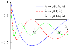
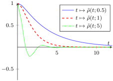
Figure 2: Graphs for the function $\tilde{\rho}$ for the value $b=2$. The non-monotonicity of the functions $t\mapsto\tilde{\rho}(t;\lambda)$ and $\lambda\mapsto\tilde{\rho}(t;\lambda)$ requires to compare the rates with the regularisation methods derived from the envelope.

To see that this solution gives rise to a regularisation method as introduced in Section 2, we first verify that the function $\lambda\mapsto\tilde{\rho}(t;\lambda)$, which corresponds to the error function $\tilde{r}_{\alpha}$ in Section 2, is non-negative and monotonically decreasing for sufficiently small values of $\lambda$ as required for $\tilde{r}_{\alpha}$ in Section 2 (ii).

Lemma 5.2.

The function $\lambda\mapsto\tilde{\rho}(t;\lambda)$ defined by Equation 5.2 is for every $t\in(0,\infty)$ non-negative and monotonically decreasing on the interval $(0,\frac{b^{2}}{4}+\frac{\pi^{2}}{4t^{2}})$.

Proof:

We proof this separately for $\lambda\in(0,\tfrac{b^{2}}{4})$ and for $\lambda\in(\frac{b^{2}}{4},\frac{b^{2}}{4}+\frac{\pi^{2}}{4t^{2}})$.

• We remark that the function

  $$g_{\tau}\colon(0,\infty)\to\mathds{R},\;g_{\tau}(\beta)=\cosh(\beta\tau)+\frac{\sinh(\beta\tau)}{\beta},$$

  is non-negative and fulfils for arbitrary $\tau>0$ that

  $$g_{\tau}^{\prime}(\beta)=\tau\sinh(\beta\tau)+\frac{\tau\cosh(\beta\tau)}{\beta}-\frac{\sinh(\beta\tau)}{\beta^{2}}=\tau\sinh(\beta\tau)+\frac{\cosh(\beta\tau)}{\beta^{2}}(\beta\tau-\tanh(\beta\tau))\geq 0,$$

  since $\tanh(z)\leq z$ for all $z\geq 0$. Thus, writing the function $\tilde{\rho}$ for $\lambda\in(0,\frac{b^{2}}{4})$ with the function $\beta_{-}$ given by Equation 5.3 in the form

  $$\tilde{\rho}(t;\lambda)=\mathrm{e}^{-\frac{bt}{2}}g_{\frac{bt}{2}}(\beta_{-}(\lambda)),$$

  we find that

  $$\partial_{\lambda}\tilde{\rho}(t;\lambda)=\mathrm{e}^{-\frac{bt}{2}}g_{\frac{bt}{2}}^{\prime}(\beta_{-}(\lambda))\beta_{-}^{\prime}(\lambda)\leq 0,$$

  since $\beta_{-}^{\prime}(\lambda)=-\frac{2}{b^{2}\beta_{-}(\lambda)}\leq 0$. Therefore, the function $\lambda\mapsto\tilde{\rho}(t;\lambda)$ is non-negative and monotonically decreasing on $(0,\frac{b^{2}}{4})$.

• Similarly, we consider for $\lambda\in(\frac{b^{2}}{4},\infty)$ the function

  $$G_{\tau}\colon(0,\infty)\to\mathds{R},\;G_{\tau}(\beta)=\cos(\beta\tau)+\frac{\sin(\beta\tau)}{\beta},$$

  for arbitrary $\tau>0$. Since $\lim_{\beta\to 0}G_{\tau}(\beta)=1+\tau>0$ and since the smallest zero $\beta_{\tau}$ of $G_{\tau}$ is the smallest non-negative solution of the equation $\tan(\beta\tau)=-\beta$, implying that $\beta_{\tau}\tau\in(\frac{\pi}{2},\pi)$, we have that $G_{\tau}(\beta)\geq 0$ for all $\beta\in(0,\frac{\pi}{2\tau})\subset(0,\beta_{\tau})$.

  Moreover, the derivative of $G_{\tau}$ satisfies for every $\beta\in(0,\tfrac{\pi}{2\tau})$ that

  $$G_{\tau}^{\prime}(\beta)=-\tau\sin(\beta\tau)+\frac{\tau\cos(\beta\tau)}{\beta}-\frac{\sin(\beta\tau)}{\beta^{2}}=-\frac{\cos(\beta\tau)}{\beta^{2}}\left((\beta^{2}\tau+1)\tan(\beta\tau)-\beta\tau\right)\leq 0,$$

  since $\tan(z)\geq z$ for every $z\geq 0$. Therefore, we find for the function $\tilde{\rho}$ on the domain $(0,\infty)\times(\frac{b^{2}}{4},\infty)$, where it has the form

  $$\tilde{\rho}(t;\lambda)=\mathrm{e}^{-\frac{bt}{2}}G_{\frac{bt}{2}}(\beta_{+}(\lambda))$$

  with $\beta_{+}$ given by Equation 5.3, that

  $$\tilde{\rho}(t;\lambda)\geq 0\text{ and }\partial_{\lambda}\tilde{\rho}(t;\lambda)=\mathrm{e}^{-\frac{bt}{2}}G_{\frac{bt}{2}}^{\prime}(\beta_{+}(\lambda))\beta_{+}^{\prime}(\lambda)\leq 0\text{ for }\beta_{+}(\lambda)<\frac{\pi}{bt},\text{ that is, for }\lambda<\frac{b^{2}}{4}+\frac{\pi^{2}}{4t^{2}},$$

  since $\beta_{+}^{\prime}(\lambda)=\frac{2}{b^{2}\beta_{+}(\lambda)}\geq 0$.

Because $\tilde{\rho}$ is continuous, this implies that $\lambda\mapsto\tilde{\rho}(t;\lambda)$ is for every $t\in(0,\infty)$ non-negative and monotonically decreasing on $(0,\frac{b^{2}}{4}+\frac{\pi^{2}}{4t^{2}})$. $\square$

In a next step, we introduce the function $\tilde{P}(t;\cdot)$ as a correspondence to the upper bound $\tilde{R}_{\alpha}$ and show that it fulfils the properties necessary for Section 2 (iii).

Lemma 5.3.

We define the function

$$\tilde{P}(t;\lambda)=\begin{cases}\mathrm{e}^{-\frac{bt}{2}}\left(\cosh\left(\beta_{-}(\lambda)\frac{bt}{2}\right)+\frac{1}{\beta_{-}(\lambda)}\sinh\left(\beta_{-}(\lambda)\frac{bt}{2}\right)\right)&\text{if}\;\lambda\in(0,\frac{b^{2}}{4}),\\ \mathrm{e}^{-\frac{bt}{2}}(1+\frac{bt}{2})&\text{if}\;\lambda\in[\frac{b^{2}}{4},\infty),\end{cases}$$ (5.5)

where the function $\beta_{-}$ shall be given by Equation 5.3.

Then, $\tilde{P}$ is an upper bound for the absolute value of the function $\tilde{\rho}$ defined by Equation 5.2: $\tilde{P}\geq|\tilde{\rho}|$.

Proof:

Since $\tilde{\rho}(t;\lambda)=\tilde{P}(t;\lambda)$ for $\lambda\leq\frac{b^{2}}{4}$ for every $t>0$, we only need to consider the case $\lambda>\frac{b^{2}}{4}$. Using that $\left|\cos(z)\right|\leq 1$ and $\left|\sin(z)\right|\leq|z|$ for all $z\in\mathds{R}$, we find with $\beta_{+}$ as in Equation 5.3 for every $\lambda>\frac{b^{2}}{4}$ and every $t>0$ that

$$|\tilde{\rho}(t;\lambda)|=\mathrm{e}^{-\frac{bt}{2}}\left|\cos\left(\beta_{+}(\lambda)\frac{bt}{2}\right)+\frac{1}{\beta_{+}(\lambda)}\sin\left(\beta_{+}(\lambda)\frac{bt}{2}\right)\right|\leq\mathrm{e}^{-\frac{bt}{2}}\left(1+\frac{bt}{2}\right)=\tilde{P}(t;\lambda).$$

$\square$

Lemma 5.4.

Let $\tilde{P}$ be given by Equation 5.5. Then, $\lambda\mapsto\tilde{P}(t;\lambda)$ is monotonically decreasing and $t\mapsto\tilde{P}(t;\lambda)$ is strictly decreasing.

Proof:

For the derivative of $\tilde{P}$ with respect to $t$, we get

$$\partial_{t}\tilde{P}(t;\lambda)=\begin{cases}\frac{b}{2}\mathrm{e}^{-\frac{bt}{2}}\left(\beta_{-}(\lambda)-\frac{1}{\beta_{-}(\lambda)}\right)\sinh\left(\beta_{-}(\lambda)\frac{bt}{2}\right)&\text{if }\lambda\in(0,\frac{b^{2}}{4}),\\ -\frac{b^{2}t}{4}\mathrm{e}^{-\frac{bt}{2}}&\text{if }\lambda\in[\frac{b^{2}}{4},\infty),\end{cases}$$

with $\beta_{-}$ defined in Equation 5.3; and since $\beta_{-}(\lambda)\in(0,1)$ for every $\lambda\in(0,\frac{b^{2}}{4})$, we thus have $\partial_{t}\tilde{P}(t;\lambda)<0$ for every $t>0$ and every $\lambda>0$.

Since $\tilde{P}(t;\lambda)=\tilde{\rho}(t;\lambda)$ for $\lambda\in(0,\frac{b^{2}}{4}]$, where $\tilde{\rho}$ denotes the solution of Equation 5.1, given by Equation 5.2, we already know from Lemma 5.2 that $\lambda\mapsto\tilde{P}(t;\lambda)$ is monotonically decreasing on $(0,\frac{b^{2}}{4}]$. And since $\lambda\mapsto\tilde{P}(t;\lambda)$ is constant on $[\frac{b^{2}}{4},\infty)$, it is monotonically decreasing on $(0,\infty)$. $\square$

To verify later the compatibility of the convergence rate functions $\varphi^{\mathrm{H}}_{\mu}$ and $\varphi^{\mathrm{L}}_{\mu}$ introduced in Equation 2.11 and Equation 2.12, we derive here an appropriate upper bound for $\tilde{P}$.

Lemma 5.5.

We have for every $\Lambda>0$ that the function $\tilde{P}$ defined in Equation 5.5 can be bounded from above by

$$\tilde{P}(t;\lambda)\leq\Psi_{\Lambda}(\lambda t)\text{ for all }t>0,\;\lambda\in(0,\Lambda],$$

where

$$\Psi_{\Lambda}(z)=\max\left\{2\mathrm{e}^{-\frac{z}{b}},\mathrm{e}^{-\frac{bz}{2\Lambda}}\left(1+\frac{bz}{2\Lambda}\right)\right\}.$$ (5.6)

Proof:

We consider the two cases $\lambda\in(0,\frac{b^{2}}{4})$ and $\lambda\in[\frac{b^{2}}{4},\Lambda]$ separately.

• For $\lambda\in(0,\frac{b^{2}}{4})$, we use the two inequalities $\cosh(z)\leq\mathrm{e}^{z}$ and $\frac{\sinh(z)}{z}\leq\mathrm{e}^{z}$ for all $z\geq 0$, where the latter follows from the fact that $f(z)=2z\mathrm{e}^{z}(\mathrm{e}^{z}-\frac{\sinh(z)}{z})=(2z-1)\mathrm{e}^{2z}+1$ is because of $f^{\prime}(z)=4z\mathrm{e}^{2z}\geq 0$ monotonically increasing on $[0,\infty)$ and thus fulfils $f(z)\geq f(0)=0$ for every $z\geq 0$. With this, we find from Equation 5.5 that

  $$\tilde{P}(t;\lambda)\leq 2\exp\left(\left(\sqrt{1-\frac{4\lambda}{b^{2}}}-1\right)\frac{bt}{2}\right).$$

  Since $\sqrt{1-z}\leq 1-\frac{z}{2}$ for all $z\in(0,1)$, we then obtain

  $$\tilde{P}(t;\lambda)\leq 2\mathrm{e}^{-\frac{\lambda t}{b}}\text{ for every }t>0,\;\lambda\in(0,\tfrac{b^{2}}{4}).$$

• For $\lambda\in[\frac{b^{2}}{4},\Lambda]$, we use that $t\mapsto\tilde{P}(t;\lambda)$ is according to Lemma 5.4 for every $\lambda\in(0,\infty)$ monotonically decreasing and obtain from Equation 5.5 that

  $$\tilde{P}(t;\lambda)\leq\tilde{P}\left(\frac{\lambda t}{\Lambda};\lambda\right)=\mathrm{e}^{-\frac{b\lambda t}{2\Lambda}}\left(1+\frac{b\lambda t}{2\Lambda}\right)\text{ for every }t>0.$$

$\square$

Next, we give an upper bound for the function $\rho$, $\rho(t;\lambda)\coloneqq\frac{1}{\lambda}(1-\tilde{\rho}(t;\lambda))$, which allows us to verify the property in Section 2 (i) for the corresponding generator $(r_{\alpha})_{\alpha>0}$ of the regularisation method.

Lemma 5.6.

Let $\tilde{\rho}$ be given by Equation 5.2. Then, there exists a constant $\sigma_{1}\in(0,1)$ such that

$$\frac{1}{\lambda}(1-\tilde{\rho}(t;\lambda))\leq\sigma_{1}{\sqrt{\frac{2t}{b\lambda}}}\text{ for all }t>0,\;\lambda>0.$$

Proof:

We consider the two cases for $\lambda\in(0,\frac{b^{2}}{4})$ and $\lambda\in(\frac{b^{2}}{4},\infty)$ separately. The estimate for $\lambda=\frac{b^{2}}{4}$ then follows directly from the fact that the function $\lambda\mapsto\tilde{\rho}(t;\lambda)$ is continuous for every $t\in[0,\infty)$.

• For $\lambda\in(0,\frac{b^{2}}{4})$, we use that $\cosh(z)=\mathrm{e}^{z}-\sinh(z)$ for every $z\in\mathds{R}$ and obtain with the function $\beta_{-}$ from Equation 5.3 that

  $$\frac{1}{\lambda}(1-\tilde{\rho}(t;\lambda))=\frac{1}{\lambda}\left(1-\mathrm{e}^{-(1-\beta_{-}(\lambda))\frac{bt}{2}}-\left(\frac{1}{\beta_{-}(\lambda)}-1\right)\mathrm{e}^{-\frac{bt}{2}}\sinh(\beta_{-}(\lambda)\tfrac{bt}{2})\right).$$

  Since $\beta_{-}(\lambda)\in(0,1)$, we can therefore estimate this with the help of Lemma 4.2 by

  $$\frac{1}{\lambda}(1-\tilde{\rho}(t;\lambda))\leq\frac{1}{\lambda}\left(1-\mathrm{e}^{-(1-\beta_{-}(\lambda))\frac{bt}{2}}\right)\leq\frac{\sigma_{0}}{\lambda}\sqrt{1-\beta_{-}(\lambda)}\sqrt{\frac{bt}{2}},$$

  where $\sigma_{0}\in(0,1)$ is the constant found in Lemma 4.2. Since $\lambda=\frac{b^{2}}{4}(1-\beta_{-}^{2}(\lambda))$, this means

  $$\frac{1}{\lambda}(1-\tilde{\rho}(t;\lambda))\leq\frac{\sigma_{0}}{\sqrt{1+\beta_{-}(\lambda)}}\sqrt{\frac{2t}{b\lambda}}\leq\sigma_{0}\sqrt{\frac{2t}{b\lambda}}.$$

• For $\lambda\in(\frac{b^{2}}{4},\infty)$, we remark that

  $$\partial_{t}\tilde{\rho}(t;\lambda)=-\frac{b}{2}\left(\beta_{+}(\lambda)+\frac{1}{\beta_{+}(\lambda)}\right)\mathrm{e}^{-\frac{bt}{2}}\sin\left(\beta_{+}(\lambda)\frac{bt}{2}\right),$$

  where $\beta_{+}$ is given by Equation 5.3. Since the function $[0,\infty)\to\mathds{R}$, $z\mapsto(\mathrm{e}^{-z}\sin(az))^{2}$, $a>0$, attains its maximal value at its smallest non-negative critical point $z=\frac{1}{a}\arctan(a)$, we have that

  $$\left|\partial_{t}\tilde{\rho}(t;\lambda)\right|\leq\frac{b}{2}\left(\beta_{+}(\lambda)+\frac{1}{\beta_{+}(\lambda)}\right)\mathrm{e}^{-\frac{\arctan(\beta_{+}(\lambda))}{\beta_{+}(\lambda)}}\left|\sin(\arctan(\beta_{+}(\lambda)))\right|.$$

  Using that $\sin(z)=\frac{\tan(z)}{\sqrt{1+\tan^{2}(z)}}$ for all $z\in(-\frac{\pi}{2},\frac{\pi}{2})$, this reads

  $$\left|\partial_{t}\tilde{\rho}(t;\lambda)\right|\leq\frac{b}{2}\sqrt{1+\beta_{+}^{2}(\lambda)}\,\mathrm{e}^{-\frac{\arctan(\beta_{+}(\lambda))}{\beta_{+}(\lambda)}}.$$ (5.7)

  We further realise that the function $f\colon(0,\infty)\to\mathds{R}$, $f(z)=\frac{1}{\sqrt{1+z^{2}}}\mathrm{e}^{-\frac{\arctan(z)}{z}}$, is monotonically decreasing because of

  $$f^{\prime}(z) =-\frac{1}{\sqrt{1+z^{2}}}\mathrm{e}^{-\frac{\arctan(z)}{z}}\left(\frac{z}{1+z^{2}}+\frac{1}{z(1+z^{2})}-\frac{\arctan(z)}{z^{2}}\right)$$

  $$=-\frac{1}{z^{2}\sqrt{1+z^{2}}}\mathrm{e}^{-\frac{\arctan(z)}{z}}(z-\arctan(z))\leq 0.$$

  Thus, $f(z)\leq\lim_{z\to 0}f(z)=\mathrm{e}^{-1}$ and Equation 5.7 therefore implies that

  $$\left|\partial_{t}\tilde{\rho}(t;\lambda)\right|\leq\frac{b}{2\mathrm{e}}(1+\beta_{+}^{2}(\lambda)).$$

  With $\frac{4}{b^{2}}\lambda=(1+\beta_{+}^{2}(\lambda))$, the mean value theorem therefore gives us

  $$\frac{1}{\lambda}(1-\tilde{\rho}(t;\lambda))=\frac{1}{\lambda}(\tilde{\rho}(0;\lambda)-\tilde{\rho}(t;\lambda))\leq\frac{2t}{\mathrm{e}b}\text{ for all }t>0.$$

  Since we know from Lemma 5.3 and Lemma 5.4 that we can estimate $\tilde{\rho}$ with the function $\tilde{P}$ from Equation 5.5 by

  $$|\tilde{\rho}(t;\lambda)|\leq\tilde{P}(t;\lambda)\leq\tilde{P}(0;\lambda)=1,$$ (5.8)

  we find by using the estimate $\min\{a,b\}\leq\min\{\sqrt{a},\sqrt{b}\}\max\{\sqrt{a},\sqrt{b}\}=\sqrt{ab}$ for all $a,b>0$ that

  $$\frac{1}{\lambda}(1-\tilde{\rho}(t;\lambda))\leq\min\left\{\frac{2}{\lambda},\frac{2t}{\mathrm{e}b}\right\}\leq\sqrt{\frac{2}{\mathrm{e}}}\sqrt{\frac{2t}{b\lambda}}\text{ for all }t>0.$$

$\square$

Finally, we can put together all the estimates to obtain a regularisation method corresponding to the solution $\xi$ of the heavy ball equation, Equation 1.4.

Proposition .

Let $\tilde{\rho}$ be the solution of Equation 5.1. Then, the functions $(r_{\alpha})_{\alpha>0}$,

$$r_{\alpha}(\lambda)\coloneqq\frac{1}{\lambda}(1-\tilde{\rho}(\tfrac{b}{2\alpha};\lambda)),$$ (5.9)

define a regularisation method in the sense of Section 2.

Proof:

We verify the four conditions in Section 2.

1. We have already seen in Equation 5.8 that $|\tilde{\rho}(t;\lambda)|\leq 1$ and thus $r_{\alpha}(\lambda)\leq\frac{2}{\lambda}$ for every $\lambda>0$.

   Moreover, Lemma 5.6 implies that there exists a parameter $\sigma_{1}\in(0,1)$ such that

   $$r_{\alpha}(\lambda)=\frac{1}{\lambda}(1-\tilde{\rho}(\tfrac{b}{2\alpha};\lambda))\leq\frac{\sigma_{1}}{\sqrt{\alpha\lambda}},$$

   which is Equation 2.1.

2. The corresponding error function

   $$\tilde{r}_{\alpha}\colon(0,\infty)\to[-1,1],\;\tilde{r}_{\alpha}(\lambda)=\tilde{\rho}(\tfrac{b}{2\alpha};\lambda),$$

   is according to Lemma 5.2 non-negative and monotonically decreasing on $(0,\frac{b^{2}}{4}+\frac{\pi^{2}\alpha^{2}}{b^{2}})$. Using that $a^{2}+b^{2}\geq 2ab$ for all $a,b\in\mathds{R}$, we find that

   $$\frac{b^{2}}{4}+\frac{\pi^{2}\alpha^{2}}{b^{2}}\geq 2\sqrt{\frac{\pi^{2}\alpha^{2}}{b^{2}}\,\frac{b^{2}}{4}}=\pi\alpha>\alpha,$$

   which implies that $\tilde{r}_{\alpha}$ is for every $\alpha>0$ non-negative and monotonically decreasing on $(0,\alpha)$.

3. Choosing

   $$\tilde{R}_{\alpha}(\lambda)\coloneqq\tilde{P}(\tfrac{b}{2\alpha};\lambda)$$ (5.10)

   with the function $\tilde{P}$ from Equation 5.5, we know from Lemma 5.3 that $\tilde{R}_{\alpha}(\lambda)\geq\left|\tilde{r}_{\alpha}(\lambda)\right|$ holds for all $\lambda>0$ and $\alpha>0$. Moreover, Lemma 5.4 tells us that $\tilde{R}_{\alpha}$ is for every $\alpha>0$ monotonically decreasing and that $\alpha\mapsto\tilde{R}_{\alpha}(\alpha;\lambda)$ is for every $\lambda>0$ monotonically increasing.

4. To estimate the values $\tilde{R}_{\alpha}(\alpha)$ for $\alpha$ in a neighbourhood of zero, we calculate the limit

   $$\lim_{\alpha\to 0}\tilde{R}_{\alpha}(\alpha)=\lim_{\alpha\to 0}\tilde{P}(\tfrac{b}{2\alpha};\alpha))=\lim_{\alpha\to 0}\mathrm{e}^{-\frac{b^{2}}{4\alpha}}\left(\cosh\left(\beta_{-}(\alpha)\frac{b^{2}}{4\alpha}\right)+\frac{1}{\beta_{-}(\alpha)}\sinh\left(\beta_{-}(\alpha)\frac{b^{2}}{4\alpha}\right)\right),$$

   where $\beta_{-}$ is given by Equation 5.3. Setting $\tilde{\alpha}=\frac{4\alpha}{b^{2}}$ and using that then $\beta_{-}(\alpha)=\sqrt{1-\frac{4\alpha}{b^{2}}}=\sqrt{1-\tilde{\alpha}}$, we get that

   $$\lim_{\alpha\to 0}\tilde{R}_{\alpha}(\alpha) =\lim_{\tilde{\alpha}\to 0}\mathrm{e}^{-\frac{1}{\tilde{\alpha}}}\left(\cosh\left(\frac{\sqrt{1-\tilde{\alpha}}}{\tilde{\alpha}}\right)+\frac{1}{\sqrt{1-\tilde{\alpha}}}\sinh\left(\frac{\sqrt{1-\tilde{\alpha}}}{\tilde{\alpha}}\right)\right)$$

   $$=\lim_{\tilde{\alpha}\to 0}\frac{1}{2}\left(1+\frac{1}{\sqrt{1-\tilde{\alpha}}}\right)\mathrm{e}^{\frac{\sqrt{1-\tilde{\alpha}}-1}{\tilde{\alpha}}}=\mathrm{e}^{-\frac{1}{2}}<1.$$

   Thus, there exists for an arbitrarily chosen $\tilde{\sigma}_{0}\in(\mathrm{e}^{-\frac{1}{2}},1)$ a parameter $\bar{\alpha}_{0}>0$ such that $\tilde{R}_{\alpha}(\alpha)\leq\tilde{\sigma}_{0}$ for every $\alpha\in(0,\bar{\alpha}_{0})$.

   Using further that $t\mapsto\tilde{P}(t;\lambda)$ is strictly decreasing, see Lemma 5.4, we have for every $\alpha>0$ that

   $$\tilde{R}_{\alpha}(\alpha)=\tilde{P}(\tfrac{b}{2\alpha};\alpha)<\tilde{P}(0;\alpha)=1.$$

   Thus, since $\alpha\mapsto\tilde{R}_{\alpha}(\alpha)$ is by definition of $\tilde{P}$ in Equation 5.5 continuous on $(0,\infty)$, we have for every $\bar{\alpha}>0$ that

   $$\sup_{\alpha\in(0,\bar{\alpha}]}\tilde{R}_{\alpha}(\alpha)=\max\bigg{\{}\sup_{\alpha\in(0,\bar{\alpha}_{0})}\tilde{R}_{\alpha}(\alpha),\sup_{\alpha\in[\bar{\alpha}_{0},\bar{\alpha}]}\tilde{R}_{\alpha}(\alpha)\bigg{\}}\leq\max\bigg{\{}\tilde{\sigma}_{0},\max_{\alpha\in[\bar{\alpha}_{0},\bar{\alpha}]}\tilde{R}_{\alpha}(\alpha)\bigg{\}}<1,$$

   which shows Section 2 (iv).

$\square$

To be able to apply Section 2.5 for the regularisation method generated by $(r_{\alpha})_{\alpha>0}$ from Equation 5.9 to the common convergence rates $\varphi^{\mathrm{H}}_{\mu}$ and $\varphi^{\mathrm{L}}_{\mu}$, it remains to show that they are compatible with $(r_{\alpha})_{\alpha>0}$.

Lemma 5.7.

The functions $\varphi^{\mathrm{H}}_{\mu}$ and $\varphi^{\mathrm{L}}_{\mu}$ defined in Section 2 are for all $\mu>0$ compatible with the regularisation method $(r_{\alpha})_{\alpha>0}$ defined by Equation 5.9 in the sense of Section 2.2.

Proof:

We know from Section 2.2 that we only need to prove the statement for $\varphi^{\mathrm{H}}_{\mu}$ for every $\mu>0$. The function $\tilde{R}_{\alpha}$ defined in Equation 5.10 fulfils according to Lemma 5.5 for arbitrary $\Lambda>0$ that

$$\tilde{R}_{\alpha}^{2}(\lambda)=\tilde{P}^{2}\left(\frac{b}{2\alpha};\lambda\right)\leq\Psi_{\Lambda}^{2}\left(\frac{b\lambda}{2\alpha}\right)\leq\Psi_{\Lambda}^{2}\left(\frac{b}{2}\left(\frac{\varphi^{\mathrm{H}}_{\mu}(\lambda)}{\varphi^{\mathrm{H}}_{\mu}(\alpha)}\right)^{\frac{1}{\mu}}\right)\text{ for every }\alpha>0,\;\lambda\in(0,\Lambda],$$

where $\Psi_{\Lambda}$ is given by Equation 5.6. Since $z\mapsto\Psi_{\Lambda}^{2}(\frac{b}{2}z^{\frac{1}{\mu}})$ is for every $\mu>0$ integrable, $\varphi^{\mathrm{H}}_{\mu}$ is compatible with $(r_{\alpha})_{\alpha>0}$. $\square$

We can therefore apply Section 2.5 to the regularisation method induced by Equation 1.4, which is the regularisation method generated by the functions $(r_{\alpha})_{\alpha>0}$ defined in Equation 5.9, and the convergence rate functions $\varphi^{\mathrm{H}}_{\mu}$ or $\varphi^{\mathrm{L}}_{\mu}$ for arbitrary $\mu>0$. Thus, although the functions $t\mapsto\tilde{\rho}(t;\lambda)$ and $\lambda\mapsto\tilde{\rho}(t;\lambda)$ are not monotonic, we obtain optimal convergence rates of the regularisation method under variational source conditions such as in Equation 2.28.

If we formulate it with the stronger standard source condition, see Section 2.5, we can reproduce a result similar to [33, Theorem 5.1].

Corollary .

Let $y\in\mathcal{R}(L)$ be given such that the corresponding minimum norm solution $x^{\dagger}\in\mathcal{X}$, fulfilling $Lx^{\dagger}=y$ and $\|x^{\dagger}\|=\inf\{\left\|x\right\|\mid Lx=y\}$, satisfies for some $\mu>0$ the source condition

$$x^{\dagger}\in\mathcal{R}\big{(}(L^{*}L)^{\frac{\mu}{2}}\big{)}.$$

Then, if $\xi$ is the solution of the initial value problem in Equation 1.4,

1. there exists a constant $C_{1}>0$ such that

   $$\left\|\xi(t;y)-x^{\dagger}\right\|^{2}\leq C_{1}t^{-\mu}\text{ for all }t>0;$$

2. there exists a constant $C_{2}>0$ such that

   $$\inf_{t>0}\left\|\xi(t;\tilde{y})-x^{\dagger}\right\|^{2}\leq C_{2}\left\|\tilde{y}-y\right\|^{\frac{2\mu}{\mu+1}}\text{ for all }\tilde{y}\in\mathcal{Y};$$

   and

3. there exists a constant $C_{3}>0$ such that

   $$\left\|L\xi(t;y)-y\right\|^{2}\leq C_{3}t^{-\mu-1}\text{ for all }t>0.$$

Proof:

The proof follows exactly the lines of the proof of Section 4, where the compatibility of $\varphi^{\mathrm{H}}_{\mu}$ is shown in Lemma 5.7 and we have here the slightly different scaling

$$x_{\alpha}(\tilde{y})=r_{\alpha}(L^{*}L)L^{*}\tilde{y}=\int_{(0,\left\|L\right\|^{2}]}\frac{1-\tilde{\rho}(\tfrac{b}{2\alpha};\lambda)}{\lambda}\,\mathrm{d}\mathbf{E}_{\lambda}L^{*}\tilde{y}=\xi(\tfrac{b}{2\alpha};\tilde{y})$$

between the regularised solution $x_{\alpha}$, defined in Equation 2.3 with the regularisation method $(r_{\alpha})_{\alpha>0}$ from Equation 5.9, and the solutions $\xi$ of Equation 1.4 and $\tilde{\rho}$ of Equation 5.1; which however does not cause a change in the order of the convergence rates. $\square$

6. The Vanishing Viscosity Flow

We consider now the dynamical method Equation 1.2 for $N=2$ with the variable coefficient $a_{1}(t)=\frac{b}{t}$ for some parameter $b>0$, that is, Equation 1.5. According to Section 3, the solution of Equation 1.5 is defined via the spectral integral in Equation 3.4 of $\rho(t;\lambda)=\frac{1-\tilde{\rho}(t;\lambda)}{\lambda}$, where $\tilde{\rho}$ solves for every $\lambda\in(0,\infty)$ the initial value problem

$$\partial_{tt}\tilde{\rho}(t;\lambda)+\frac{b}{t}\partial_{t}\tilde{\rho}(t;\lambda)+\lambda\tilde{\rho}(t;\lambda) =0\text{ for all }t\in\left(0,\infty\right),$$ (6.1)

$$\partial_{t}\tilde{\rho}(0;\lambda) =0,$$

$$\tilde{\rho}(0;\lambda) =1.$$

As already noted in [29, Section 3.2], we obtain a closed form in terms of Bessel functions for the solution of Equation 6.1.

Lemma 6.1.

Let $b,\lambda>0$. Then Equation 6.1 has the unique solution

$$\tilde{\rho}(t;\lambda)=u(t\sqrt{\lambda})\text{ with }u(\tau)=\left(\frac{2}{\tau}\right)^{\frac{1}{2}(b-1)}\Gamma(\tfrac{1}{2}(b+1))J_{\frac{1}{2}(b-1)}(\tau),$$ (6.2)

where $\Gamma$ is the gamma function and $J_{\nu}$ denotes the Bessel function of first kind of order $\nu\in\mathds{R}$. See Figure 3 for a sketch of the graph of the function $u$.

Proof:

We rescale Equation 6.1 by switching to the function

$$v\colon[0,\infty)\times(0,\|L\|^{2}]\to\mathds{R},\;v(\tau;\lambda)=\tau^{\kappa}\tilde{\rho}(\sigma_{\lambda}\tau;\lambda)$$ (6.3)

with some parameters $\sigma_{\lambda}\in(0,\infty)$ and $\kappa\in\mathds{R}$. The function $v$ thus has the derivatives

$$\partial_{\tau}v(\tau;\lambda)=\sigma_{\lambda}\tau^{\kappa}\partial_{t}\tilde{\rho}(\sigma_{\lambda}\tau;\lambda)+\kappa\tau^{\kappa-1}\tilde{\rho}(\sigma_{\lambda}\tau;\lambda)$$ (6.4)

and

$$\partial_{\tau\tau}v(\tau;\lambda)=\sigma_{\lambda}^{2}\tau^{\kappa}\partial_{tt}\tilde{\rho}(\sigma_{\lambda}\tau;\lambda)+2\sigma_{\lambda}\kappa\tau^{\kappa-1}\partial_{t}\tilde{\rho}(\sigma_{\lambda}\tau;\lambda)+\kappa(\kappa-1)\tau^{\kappa-2}\tilde{\rho}(\sigma_{\lambda}\tau;\lambda).$$

We use Equation 6.1 to replace the second derivative of $\tilde{\rho}$ and obtain

$$\partial_{\tau\tau}v(\tau;\lambda)=\sigma_{\lambda}(2\kappa-b)\tau^{\kappa-1}\partial_{t}\tilde{\rho}(\sigma_{\lambda}\tau;\lambda)+(\kappa(\kappa-1)-\lambda\sigma_{\lambda}^{2}\tau^{2})\tau^{\kappa-2}\tilde{\rho}(\sigma_{\lambda}\tau;\lambda),$$

which, after writing $\partial_{t}\tilde{\rho}$ and $\tilde{\rho}$ via Equation 6.4 and Equation 6.3 in terms of the function $v$, becomes the differential equation

$$\tau^{2}\partial_{\tau\tau}v(\tau;\lambda)+(b-2\kappa)\tau\partial_{\tau}v(\tau;\lambda)+(\lambda\sigma_{\lambda}^{2}\tau^{2}-\kappa(\kappa-1)-\kappa(b-2\kappa))v(\tau;\lambda)=0$$

for the function $v$. Choosing now $\kappa=\frac{1}{2}(b-1)$, so that $b-2\kappa=1$, and $\sigma_{\lambda}=\frac{1}{\sqrt{\lambda}}$, we end up with Bessel’s differential equation

$$\tau^{2}\partial_{\tau\tau}v(\tau;\lambda)+\tau\partial_{\tau}v(\tau;\lambda)+(\tau^{2}-\kappa^{2})v(\tau;\lambda)=0,$$

for which every solution can be written as

$$v(\tau;\lambda)=\begin{cases}C_{1,\kappa}J_{|\kappa|}(\tau)+C_{2,\kappa}Y_{|\kappa|}(\tau),&\kappa\in\mathds{Z},\\ C_{1,\kappa}J_{|\kappa|}(\tau)+C_{2,\kappa}J_{-|\kappa|}(\tau),&\kappa\in\mathds{R}\setminus\mathds{Z},\end{cases}$$

for some constants $C_{1,\kappa},C_{2,\kappa}\in\mathds{R}$, where $J_{\nu}$ and $Y_{\nu}$ denote the Bessel functions of first and second kind of order $\nu\in\mathds{R}$, respectively; see, for example, [1, Chapter 9.1].

We can therefore write the solution $\tilde{\rho}$ as

$$\tilde{\rho}(t;\lambda)=\begin{cases}C_{1,\kappa}(t\sqrt{\lambda})^{-\kappa}J_{|\kappa|}(t\sqrt{\lambda})+C_{2,\kappa}(t\sqrt{\lambda})^{-\kappa}Y_{|\kappa|}(t\sqrt{\lambda}),&\kappa\in\mathds{Z},\\ C_{1,\kappa}(t\sqrt{\lambda})^{-\kappa}J_{|\kappa|}(t\sqrt{\lambda})+C_{2,\kappa}(t\sqrt{\lambda})^{-\kappa}J_{-|\kappa|}(t\sqrt{\lambda}),&\kappa\in\mathds{R}\setminus\mathds{Z}.\end{cases}$$ (6.5)

To determine the constants $C_{1,\kappa}$ and $C_{2,\kappa}$ from the initial conditions, we remark that the Bessel functions have for all $\kappa\in\mathds{R}\setminus(-\mathds{N})$ and all $n\in\mathds{N}$ asymptotically for $\tau\to 0$ the behaviour

$$\tau^{-\kappa}J_{\kappa}(\tau)=\frac{1}{2^{\kappa}\Gamma(\kappa+1)}+\mathcal{O}(\tau^{2}),\;\lim_{\tau\to 0}\tau^{n}Y_{n}(\tau)=-\frac{2^{n}(n-1)!}{\pi},\text{ and }\lim_{\tau\to 0}\frac{Y_{0}(\tau)}{\log(\tau)}=\frac{2}{\pi},$$ (6.6)

see, for example, [1, Formulae 9.1.10 and 9.1.11].

We consider the cases $\kappa\geq 0$ and $\kappa\in(-\frac{1}{2},0)$ separately.

• In particular, the relations in Equation 6.6 imply that, for the last terms in Equation 6.5, we have with $\tau=t\sqrt{\lambda}$ asymptotically for $\tau\to 0$

  • for $\kappa=0$:

    $$C_{2,0}Y_{0}(\tau)=\frac{2}{\pi}C_{2,0}\mathcal{O}(\log(\tau))$$

    because of the third relation in Equation 6.6;

  • for $\kappa\in\mathds{N}$:

    $$C_{2,\kappa}\tau^{-\kappa}Y_{\kappa}(\tau)=C_{2,\kappa}\tau^{-2\kappa}(\tau^{\kappa}Y_{\kappa}(\tau))=C_{2,\kappa}\left(-\frac{2^{\kappa}(\kappa-1)!}{\pi}+o(1)\right)\tau^{-2\kappa}$$

    because of the second relation in Equation 6.6; and

  • for $\kappa\in(0,\infty)\setminus\mathds{N}$:

    $$C_{2,\kappa}\tau^{-\kappa}J_{-\kappa}(\tau)=C_{2,\kappa}\tau^{-2\kappa}(\tau^{\kappa}J_{-\kappa}(\tau))=C_{2,\kappa}\left(\frac{2^{\kappa}}{\Gamma(1-\kappa)}+\mathcal{O}(\tau^{2})\right)\tau^{-2\kappa}$$

    because of the first relation in Equation 6.6.

  Thus, the last terms in Equation 6.5 diverge for every $\kappa\geq 0$ as $t\to 0$.

  Since the first terms in Equation 6.5 converge according to the first relation in Equation 6.6 for $t\to 0$, the initial condition $\tilde{\rho}(0;\lambda)=1$ can only be fulfilled if the coefficients $C_{2,\kappa}$, $\kappa\geq 0$, in front of the singular terms are all zero so that we have

  $$\tilde{\rho}(t;\lambda)=C_{1,\kappa}(t\sqrt{\lambda})^{-\kappa}J_{\kappa}(t\sqrt{\lambda})\text{ for all }\kappa\geq 0.$$

  Furthermore, the initial condition $\tilde{\rho}(0;\lambda)=1$ implies according to the first relation in Equation 6.6 that

  $$C_{1,\kappa}=2^{\kappa}\Gamma(\kappa+1)\text{ for all }\kappa\geq 0,$$

  which gives the representation of Equation 6.2 for the solution $\tilde{\rho}$.

  It remains to check that also the initial condition $\partial_{t}\tilde{\rho}(0;\lambda)=0$ is for all $\kappa\geq 0$ fulfilled, which again follows directly from the first relation in Equation 6.6:

  $$\partial_{t}\tilde{\rho}(0;\lambda)=\lim_{t\to 0}\frac{1}{t}\left(2^{\kappa}\Gamma(\kappa+1)(t\sqrt{\lambda})^{-\kappa}J_{\kappa}(t\sqrt{\lambda})-1\right)=0\text{ for all }\kappa\geq 0.$$

• For $\kappa\in(-\frac{1}{2},0)$, we have that the first term in $\tilde{\rho}(t;\lambda)$ converges for $t\to 0$ to $0$ because of

  $$C_{1,\kappa}(t\sqrt{\lambda})^{|\kappa|}J_{|\kappa|}(t\sqrt{\lambda})=C_{1,\kappa}(t\sqrt{\lambda})^{2|\kappa|}\left(\frac{1}{2^{|\kappa|}\Gamma(|\kappa|+1)}+\mathcal{O}(t^{2})\right),$$

  which follows from the first relation of Equation 6.6. Therefore, the initial condition $\tilde{\rho}(0;\lambda)=1$ requires that

  $$1=\tilde{\rho}(0;\lambda)=C_{2,\kappa}\lim_{t\to 0}(t\sqrt{\lambda})^{|\kappa|}J_{-|\kappa|}(t\sqrt{\lambda})\text{ for all }\kappa\in(-\tfrac{1}{2},0),$$

  from which we get with the first property in Equation 6.6 that

  $$C_{2,\kappa}=2^{\kappa}\Gamma(\kappa+1).$$

  To determine the coefficient $C_{1,\kappa}$, we remark that the first identity in Equation 6.6 then gives us for $t\to 0$ the asymptotic behaviour

  $$\tilde{\rho}(t;\lambda)=1+C_{1,\kappa}\frac{(t\sqrt{\lambda})^{2|\kappa|}}{2^{|\kappa|}\Gamma(|\kappa|+1)}+\mathcal{O}(t^{2}).$$

  Therefore, we have for the first derivative at $t=0$ the expression

  $$\partial_{t}\tilde{\rho}(0;\lambda)=\lim_{t\to 0}C_{1,\kappa}\frac{2|\kappa|\lambda^{|\kappa|}}{2^{|\kappa|}\Gamma(|\kappa|+1)}\,\frac{1}{t^{1-2|\kappa|}}.$$

  To satisfy the initial condition $\partial_{t}\tilde{\rho}(0;\lambda)=0$, we thus have to choose $C_{1,\kappa}=0$ for $\kappa\in(-\frac{1}{2},0)$, which leaves us again with Equation 6.2.

$\square$

Figure 3: Graph of the function $u$, defined in Equation 6.2, which gives the solution $\tilde{\rho}$ of Equation 6.1 via $\tilde{\rho}(t;\lambda)=u(t\sqrt{\lambda})$. As in the heavy ball method, the function $\tilde{\rho}$ is not monotonic (in either component) so that we used the envelope of the regularisation method to obtain the optimal convergence rates.

Corollary .

The unique solution $\xi\colon[0,\infty)\times\mathcal{Y}\to\mathds{R}$ of the vanishing viscosity flow, Equation 1.5, which is twice continuously differentiable with respect to $t$ is given by

$$\xi(t;\tilde{y})=\int_{(0,\left\|L\right\|^{2}]}\frac{1-u(t\sqrt{\lambda})}{\lambda}\,\mathrm{d}\mathbf{E}_{\lambda}L^{*}\tilde{y}$$

where the function $u$ is defined by Equation 6.2.

Proof:

We have already seen in Lemma 6.1 that Equation 6.1 has the unique solution $\tilde{\rho}$ given by $\tilde{\rho}(t;\lambda)=u(t\sqrt{\lambda})$. To apply Section 3, it is thus enough to show that $\tilde{\rho}$ is smooth.

Since the function $u$ has the representation

$$u(\tau)=v(\tau^{2})\text{ with }v(\tilde{\tau})=\Gamma(\tfrac{1}{2}(b+1))\sum_{k=0}^{\infty}\frac{(-\frac{1}{4}\tilde{\tau})^{k}}{k!\Gamma(\frac{1}{2}(b+1)+k)},$$

see, for example, [1, Formula 9.1.10], the solution $\tilde{\rho}\colon[0,\infty)\times[0,\infty)\to\mathds{R}$ given by Equation 6.2 is of the form $\tilde{\rho}(t;\lambda)=u(t\sqrt{\lambda})=v(\lambda t^{2})$ and is therefore seen to be smooth. Therefore, Section 3 yields the claim. $\square$

Again, we want to determine a corresponding regularisation method. We start by showing that the function $\lambda\mapsto\tilde{\rho}(t;\lambda)$, which corresponds to the error function $\tilde{r}_{\alpha}$ of the regularisation method, is non-negative and monotonically decreasing for sufficiently small values $\lambda$ as required for $\tilde{r}_{\alpha}$ in Section 2 (ii).

Lemma 6.2.

Let $j_{\kappa,1}\in(0,\infty)$ denote the first positive zero of the Bessel function $J_{\kappa}$. Then, the solution $\tilde{\rho}$ given in Equation 6.2 fulfils

• for every $\lambda>0$ that the function $t\mapsto\tilde{\rho}(t;\lambda)$ is strictly decreasing on the interval $(0,\frac{1}{\sqrt{\lambda}}j_{\frac{1}{2}(b-1),1})$ and

• for every $t>0$ that the function $\lambda\mapsto\tilde{\rho}(t;\lambda)$ is strictly decreasing on the interval $(0,\frac{1}{t^{2}}j_{\frac{1}{2}(b-1),1}^{2})$.

Proof:

Since we can write $\tilde{\rho}$ in the form $\tilde{\rho}(t;\lambda)=u(t\sqrt{\lambda})$, see Equation 6.2, it is enough to show that

$$u^{\prime}(\tau)<0\text{ for }\tau\in(0,j_{\frac{1}{2}(b-1),1}).$$

This property of $u$ follows directly from the representation of the Bessel functions $J_{\kappa}$, $\kappa\in(-\frac{1}{2},\infty)$, as an infinite product, see, for example, [1, Formula 9.5.10]:

$$J_{\kappa}(\tau)=\frac{\tau^{\kappa}}{2^{\kappa}\Gamma(\kappa+1)}\prod_{\ell=1}^{\infty}\left(1-\frac{\tau^{2}}{j_{\kappa,\ell}^{2}}\right),$$

where $j_{\kappa,\ell}$ denotes the $\ell$th positive zero (sorted in increasing order) of $J_{\kappa}$; since this gives

$$u(\tau)=\prod_{\ell=1}^{\infty}\left(1-\frac{\tau^{2}}{j_{\frac{1}{2}(b-1),\ell}^{2}}\right),$$

which is for $\tau\in(0,j_{\frac{1}{2}(b-1),1})$ a product of only positive factors. Therefore, we have

$$u^{\prime}(\tau)=-2\tau\sum_{\ell=1}^{\infty}\left[j_{\frac{1}{2}(b-1),\ell}^{-2}\prod_{\tilde{\ell}\in\mathds{N}\setminus\{\ell\}}\left(1-\frac{\tau^{2}}{j_{\frac{1}{2}(b-1),\tilde{\ell}}^{2}}\right)\right]<0\text{ for all }\tau\in(0,j_{\frac{1}{2}(b-1),1}).$$

$\square$

Furthermore, we can construct an upper bound $\tilde{P}(t;\lambda)=U(t\sqrt{\lambda})$ of $|\tilde{\rho}(t;\lambda)|$, which corresponds to the envelope value $\tilde{R}_{\alpha}(\lambda)$, such that $\tilde{P}(t;\cdot)$ is monotonically decreasing. This will give us the condition of Section 2 (iii) for the function $\tilde{R}_{\alpha}$. The additionally derived explicit upper bound for $U$ helps us to show the compatibility of the convergence rate functions $\varphi^{\mathrm{H}}_{\mu}$ and $\varphi^{\mathrm{L}}_{\mu}$.

Lemma 6.3.

Let $\tilde{\rho}$ be the solution of Equation 6.1 given by Equation 6.2. Then, there exist a constant $C>0$ and a continuous, monotonically decreasing function $U\colon[0,\infty)\to[0,1]$ so that

• $|\tilde{\rho}(t;\lambda)|\leq U(t\sqrt{\lambda})$ for every $t\geq 0$, $\lambda>0$,

• $U(\tau)<1$ for all $\tau>0$, and

• $U(\tau)\leq C\tau^{-\frac{b}{2}}$ for all $\tau>0$.

Proof:

We use again the function $u$ defined in Equation 6.2 which satisfies $\tilde{\rho}(t;\lambda)=u(t\sqrt{\lambda})$. Then, we remark that the energy

$$E(\tau)\coloneqq{u^{\prime}}^{2}(\tau)+u^{2}(\tau),\;\tau\geq 0,$$

fulfils (using Equation 6.1 with $\lambda=1$, $t=\tau$ and $u(\tau)=\tilde{\rho}(\tau;1)$)

$$E^{\prime}(\tau)=2u^{\prime}(\tau)\left(u^{\prime\prime}(\tau)+u(\tau)\right)=-\frac{b}{\tau}{u^{\prime}}^{2}(\tau)\leq 0.$$

Since we know from Lemma 6.2 that $u^{\prime}(\tau)=\partial_{t}\tilde{\rho}(\tau;1)<0$ for $\tau\in(0,j_{\frac{1}{2}(b-1),1})$, we have that $E$ is strictly decreasing on $(0,j_{\frac{1}{2}(b-1),1})$ so that $E(j_{\frac{1}{2}(b-1),1})<E(0)$. For $\tau\geq j_{\frac{1}{2}(b-1),1}$, we can therefore estimate $u$ by

$$u^{2}(\tau)\leq E(\tau)\leq E(j_{\frac{1}{2}(b-1),1})<E(0)=1.$$

Thus, $u$ is monotonically decreasing on $(0,j_{\frac{1}{2}(b-1),1})$ and uniformly bounded by $E(j_{\frac{1}{2}(b-1),1})<1$ on $[j_{\frac{1}{2}(b-1),1},\infty)$. Therefore, we can find a monotonically decreasing function $\tilde{U}\colon[0,\infty)\to[0,1]$ with

$$u(\tau)\leq\tilde{U}(\tau)<1\text{ for every }\tau>0.$$

Since it follows from [1, Formula 9.2.1] that there exists a constant $c>0$ such that

$$|J_{\frac{1}{2}(b-1)}(\tau)|\leq c\tau^{-\frac{1}{2}}\text{ for all }\tau>0,$$

which implies according to Equation 6.2 with $C=2^{\frac{1}{2}(b-1)}\Gamma(\frac{1}{2}(b+1))c$ the upper bound

$$|u(\tau)|\leq C\tau^{-\frac{b}{2}}\text{ for all }\tau>0,$$

the function $U$ defined by $U(\tau)=\min\{\tilde{U}(\tau),C\tau^{-\frac{b}{2}}\}$ satisfies all the properties. $\square$

To verify the condition in Section 2 (i) for $r_{\alpha}$, we establish here the corresponding lower bound for the function $\tilde{\rho}$.

Lemma 6.4.

Let $\tilde{\rho}$ be the solution of Equation 6.1 given by Equation 6.2. Then, there exists a constant $\tau_{b}\in(0,j_{\frac{1}{2}(b-1),1}]$ such that

$$\tilde{\rho}(t;\lambda)\geq 1-\frac{t\sqrt{\lambda}}{2\tau_{b}}\text{ for all }t\geq 0,\;\lambda>0.$$ (6.7)

Proof:

We define $u$ again by Equation 6.2 and choose some arbitrary $c>0$. Then, the initial conditions $u(0)=1$ and $u^{\prime}(0)=0$ imply that we find a $\bar{\tau}>0$ such that $u(\tau)\geq 1-c\tau$ for all $\tau\in[0,\bar{\tau}]$. Setting now $\tau_{b}\coloneqq\min\{\frac{1}{2c},\frac{\bar{\tau}}{4},j_{\frac{1}{2}(b-1),1}\}$, we have by construction

$$u(\tau)\geq 1-c\tau\geq 1-\frac{\tau}{2\tau_{b}}\text{ for all }\tau\in[0,\bar{\tau}].$$

Moreover, the uniform bound $\left|u(\tau)\right|<1$ for all $\tau>0$, shown in Lemma 6.3, implies that

$$u(\tau)>-1\geq 1-\frac{2}{\bar{\tau}}\tau\geq 1-\frac{\tau}{2\tau_{b}}\text{ for all }\tau\in[\bar{\tau},\infty).$$

Thus, $\tilde{\rho}(t;\lambda)=u(t\sqrt{\lambda})$ yields the claim. $\square$

These estimates for $\tilde{\rho}$ suffice now to show that the functions $r_{\alpha}$ defined by Equation 6.8 generate the regularisation method corresponding to the solution $\xi$ of Equation 1.5.

Proposition .

Let $\tilde{\rho}$ be the solution of Equation 6.1 given by Equation 6.2, $\tau_{b}$ be the constant defined in Lemma 6.4, and set

$$r_{\alpha}(\lambda)\coloneqq\frac{1}{\lambda}\left(1-\tilde{\rho}\left(\frac{\tau_{b}}{\sqrt{\alpha}};\lambda\right)\right).$$ (6.8)

Then, $(r_{\alpha})_{\alpha>0}$ generates a regularisation method in the sense of Section 2.

Proof:

We verify the four conditions in Section 2.

1. We know from Lemma 6.3 that $|\tilde{\rho}|\leq 1$, and thus it follows that

   $$r_{\alpha}(\lambda)\leq\frac{2}{\lambda}.$$

   Moreover, it follows from Equation 6.7 that

   $$r_{\alpha}(\lambda)=\frac{1}{\lambda}\left(1-\tilde{\rho}\left(\frac{\tau_{b}}{\sqrt{\alpha}};\lambda\right)\right)\leq\frac{1}{2\sqrt{\alpha\lambda}}.$$

2. The error function $\tilde{r}_{\alpha}$ corresponding to the generator $r_{\alpha}$ is given by

   $$\tilde{r}_{\alpha}(\lambda)=\tilde{\rho}\left(\frac{\tau_{b}}{\sqrt{\alpha}};\lambda\right),$$

   which is a monotonically decreasing function on $(0,\frac{1}{\tau_{b}^{2}}j_{\frac{1}{2}(b-1),1}^{2}\alpha)$ according to Lemma 6.2. Since we have chosen $\tau_{b}\in(0,j_{\frac{1}{2}(b-1),1}]$, see Lemma 6.4, this in particular shows that $\tilde{r}_{\alpha}$ is monotonically decreasing on $(0,\alpha)$.

3. Let $U$ be the function constructed in Lemma 6.3. We define

   $$\tilde{R}_{\alpha}(\lambda)\coloneqq U\left(\tau_{b}\sqrt{\frac{\lambda}{\alpha}}\right).$$ (6.9)

   Then, we have by Lemma 6.3 that $\lambda\mapsto\tilde{R}_{\alpha}(\lambda)$ is monotonically decreasing, $\alpha\mapsto\tilde{R}_{\alpha}(\lambda)$ is continuous and monotonically increasing and $\tilde{R}_{\alpha}$ fulfils

   $$\tilde{r}_{\alpha}(\lambda)=\tilde{\rho}\left(\frac{\tau_{b}}{\sqrt{\alpha}};\lambda\right)\leq U\left(\tau_{b}\sqrt{\frac{\lambda}{\alpha}}\right)=\tilde{R}_{\alpha}(\lambda).$$

4. We have again by Lemma 6.3 that

   $$\tilde{R}_{\alpha}(\alpha)=U(\tau_{b})<1\text{ for all }\alpha>0.$$

$\square$

As before, we also verify that the classical convergence rate functions $\varphi^{\mathrm{H}}_{\mu}$ and $\varphi^{\mathrm{L}}_{\mu}$ are compatible with the regularisation method $(r_{\alpha})_{\alpha>0}$. In contrast to Showalter’s method and the heavy ball method, the compatibility for $\varphi^{\mathrm{H}}_{\mu}$ only holds up to a certain saturation value for the parameter $\mu$.

Lemma 6.5.

The functions $\varphi^{\mathrm{H}}_{\mu}$ for all $\mu\in(0,\frac{b}{2})$ and the functions $\varphi^{\mathrm{L}}_{\mu}$ for all $\mu>0$, as defined in Section 2, are compatible with the regularisation method $(r_{\alpha})_{\alpha>0}$ defined by Equation 6.8 in the sense of Section 2.2.

Proof:

As before, it is because of Section 2.2 enough to check this for the functions $\varphi^{\mathrm{H}}_{\mu}$, $\mu\in(0,\frac{b}{2})$. The function $\tilde{R}_{\alpha}$ defined in Equation 6.9 fulfils according to Lemma 6.3 that there exists a constant $C>0$ with

$$\tilde{R}_{\alpha}^{2}(\lambda)=U^{2}\left(\tau_{b}\sqrt{\frac{\lambda}{\alpha}}\right)\leq C^{2}\tau_{b}^{-b}\left(\frac{\lambda}{\alpha}\right)^{-\frac{b}{2}}\leq C^{2}\tau_{b}^{-b}\left(\frac{\varphi^{\mathrm{H}}_{\mu}(\lambda)}{\varphi^{\mathrm{H}}_{\mu}(\alpha)}\right)^{-\frac{b}{2\mu}},$$

which is Equation 2.16 with the compatibility function $F_{\mu}(z)=C^{2}\tau_{b}^{-b}z^{-\frac{b}{2\mu}}$. It remains to check that $F_{\mu}\colon[1,\infty)\to\mathds{R}$ is integrable, which is the case for $\mu<\frac{b}{2}$. $\square$

We can therefore apply Section 2.5 to the regularisation method generated by the functions $(r_{\alpha})_{\alpha>0}$ defined in Equation 6.8 and the convergence rates $\varphi^{\mathrm{H}}_{\mu}$, $\mu\in(0,\frac{b}{2})$, and $\varphi^{\mathrm{L}}_{\mu}$, $\mu>0$. By using that we have by construction $x_{\alpha}(\tilde{y})=\xi(\frac{\tau_{b}}{\sqrt{\alpha}};\tilde{y})$, see Equation 6.10 below, this gives us equivalent characterisations for convergence rates of the flow $\xi$ of Equation 1.5. As before for Showalter’s method and the heavy ball method, we formulate the resulting convergence rates under the stronger, but more commonly used standard source condition, see Section 2.5.

Corollary .

Let $y\in\mathcal{R}(L)$ be given such that the corresponding minimum norm solution $x^{\dagger}\in\mathcal{X}$, fulfilling $Lx^{\dagger}=y$ and $\|x^{\dagger}\|=\inf\{\left\|x\right\|\mid Lx=y\}$, satisfies for some $\mu\in(0,\frac{b}{2})$ the source condition

$$x^{\dagger}\in\mathcal{R}\big{(}(L^{*}L)^{\frac{\mu}{2}}\big{)}.$$

Then, if $\xi$ is the solution of the initial value problem in Equation 1.5,

1. there exists a constant $C_{1}>0$ such that

   $$\left\|\xi(t;y)-x^{\dagger}\right\|^{2}\leq\frac{C_{1}}{t^{2\mu}}\text{ for all }t>0;$$

2. there exists a constant $C_{2}>0$ such that

   $$\inf_{t>0}\left\|\xi(t;\tilde{y})-x^{\dagger}\right\|^{2}\leq C_{2}\left\|\tilde{y}-y\right\|^{\frac{2\mu}{\mu+1}}\text{ for all }\tilde{y}\in\mathcal{Y};$$

   and

3. if $\mu<\frac{b}{2}-1$, there exists a constant $C_{3}>0$ such that

   $$\left\|L\xi(t;y)-y\right\|^{2}\leq\frac{C_{3}}{t^{2(\mu+1)}}\text{ for all }t>0.$$

Proof:

The proof follows exactly the lines of the proof of Section 4, where the compatibility of $\varphi^{\mathrm{H}}_{\mu}$ is shown in Lemma 6.5 and we have the different scaling

$$x_{\alpha}(\tilde{y})=r_{\alpha}(L^{*}L)L^{*}\tilde{y}=\int_{(0,\left\|L\right\|^{2}]}\frac{1}{\lambda}\left(1-\tilde{\rho}\left(\frac{\tau_{b}}{\sqrt{\alpha}};\lambda\right)\right)\,\mathrm{d}\mathbf{E}_{\lambda}L^{*}\tilde{y}=\xi\left(\frac{\tau_{b}}{\sqrt{\alpha}};\tilde{y}\right)$$ (6.10)

between the regularised solution $x_{\alpha}$, defined in Equation 2.3 with the regularisation method $(r_{\alpha})_{\alpha>0}$ from Equation 6.8, and the solutions $\xi$ of Equation 1.5 and $\tilde{\rho}$ of Equation 6.1. Following Section 4 and using the notation $d$ from Equation 2.8 and $\tilde{d}$ from Equation 2.9 we get

1. in the case of exact data the convergence rates

   $$\left\|\xi(t;y)-x^{\dagger}\right\|^{2}=\left\|x_{\tau_{b}^{2}t^{-2}}(y)-x^{\dagger}\right\|^{2}=d\left(\frac{\tau_{b}^{2}}{t^{2}}\right)\text{ and }\left\|x_{\tau_{b}^{2}t^{-2}}(y)-x^{\dagger}\right\|^{2}\leq\frac{C_{d}\tau_{b}^{2\mu}}{t^{2\mu}}.$$

2. For perturbed data we get the convergence rate

   $$\inf_{t>0}\left\|\xi(t;\tilde{y})-x^{\dagger}\right\|^{2}=\inf_{\alpha>0}\left\|\xi\left(\frac{\tau_{b}}{\sqrt{\alpha}};\tilde{y}\right)-x^{\dagger}\right\|^{2}\leq\tilde{d}(\left\|\tilde{y}-y\right\|)\leq C_{\tilde{d}}\left\|\tilde{y}-y\right\|^{\frac{2\mu}{\mu+1}}.$$

3. Moreover, using that for $\mu<\frac{b}{2}-1$ also $\varphi^{\mathrm{H}}_{\mu+1}$ is compatible with $(r_{\alpha})_{\alpha>0}$, we get from Section 2.6 the convergence rate

   $$\left\|L\xi(t;y)-y\right\|^{2}=\left\|Lx_{\tau_{b}^{2}t^{-2}}(y)-y\right\|^{2}=q\left(\frac{\tau_{b}^{2}}{t^{2}}\right)\leq C\tau_{b}^{2(\mu+1)}t^{-2(\mu+1)}$$

   for the noise free residual error, where $q$ is defined in Equation 2.10.

$\square$

We end this section by a few remarks.

Remark (Comparison of Flows):

Comparing the results in Section 4, Section 5, and Section 6, we see that the three methods we have analysed, namely Showalter’s method, the heavy ball dynamics, and the vanishing viscosity flow, all give the same rate of convergence for noisy data with optimal stopping time. However, one should notice that their optimal stopping times are different. This is due to the acceleration property of the vanishing viscosity flow in comparison with the other two, which has been analysed in the literature.

Remark (Saturation of Viscosity Flow):

The vanishing viscosity flow suffers from a saturation effect for the convergence rate functions $\varphi^{\mathrm{H}}_{\mu}$ allowing only convergence rates up to certain values of $\mu$, which is not the case in the other two methods (because of their exponential decay of the error function at every fixed spectral value).

Remark (Comparison with literature):

Equation 6.1 has been investigated quite heavily in a more general context of non-smooth, convex functionals $\mathcal{J}$ and abstract ordinary differential equations of the form

$$\xi^{\prime\prime}(t)+\frac{b}{t}\xi^{\prime}(t)+\partial\mathcal{J}(\xi(t)) \ni 0\text{ for all }t\in\left(0,\infty\right),$$ (6.11)

$$\xi^{\prime}(0) =0,$$

$$\xi(0) =0,$$

see for instance [29, 5, 6, 7, 4]. Equation 6.11 corresponds to Equation 1.2 with $N=2$ and $a_{1}(t)=\frac{b}{t}$, $b>0$, for the particular energy functional $\mathcal{J}(x)=\frac{1}{2}\left\|Lx-y\right\|^{2}$.

The authors prove optimality of Equation 6.11, which, however, is a different term than in our paper:

1. In the above referenced paper optimality is considered with respect to all possible smooth and convex functionals $\mathcal{J}$, while in our work optimality is considered with respect to all possible variations of $y$ only. The papers [29, 7, 4] consider a finite dimensional setting where $\mathcal{J}$ maps a subset of a finite dimensional space $\mathds{R}^{d}$ into the extended reals.

2. The second difference in the optimality results is that we consider primarily optimal convergence rate of $\xi(t)-x^{\dagger}$ for $t\to\infty$ and not of $\mathcal{J}(\xi(t))\to\min_{x\in\mathcal{X}}\mathcal{J}(x)$, that is, we are considering rates in the domain of $L$, while in the referenced papers convergence in the image domain is considered. Consequently, we get rates for the residual squared (which is the rate of $J(\xi(t))$ in the referenced papers), which are based on optimal rates (in the sense of this paper) for $\xi(t)-x^{\dagger}\to 0$. The presented rates in the image domain are, however, not necessarily optimal.

Nevertheless, it is very interesting to note that the two cases $b\geq 3$ and $0<b<3$, referred to as heavy and low friction cases, do not result in a different analysis in our paper, compared to, for instance, [4]. This is of course not a contradiction, because we consider a different optimality terminology.

Conclusions

The paper shows that the dynamical flows provide optimal regularisation methods (in the sense explained in Section 2). We proved optimal convergence rates of the solutions of the flows to the minimum norm solution for $t\to\infty$ and we also provide convergence rates of the residuals of the regularised solutions.

We observed that the vanishing viscosity method, heavy ball dynamics, and Showalter’s method provide optimal reconstructions for different times. In fact, eventually, for a fair numerical comparison of the results of all three methods one should compare the results of Showalter’s method and the heavy ball dynamics, respectively, at time $t_{0}^{2}$ with the vanishing viscosity flow at time $t_{0}$.

Acknowledgements

• RB acknowledges support from the Austrian Science Fund (FWF) within the project I2419-N32 (Employing Recent Outcomes in Proximal Theory Outside the Comfort Zone).

• GD is funded by the Deutsche Forschungsgemeinschaft (DFG, German Research Foundation) under Germany’s Excellence Strategy “The Berlin Mathematics Research Center MATH” (EXC-2046/1, project ID: 390685689).

• PE and OS are supported by the Austrian Science Fund (FWF), with SFB F68, project F6804-N36 (Quantitative Coupled Physics Imaging) and project F6807-N36 (Tomography with Uncertainties).

• OS acknowledges support from the Austrian Science Fund (FWF) within the national research network Geometry and Simulation, project S11704 (Variational Methods for Imaging on Manifolds) and I3661-N27 (Novel Error Measures and Source Conditions of Regularization Methods for Inverse Problems).

References

References

- [1] M. Abramowitz and I.A. Stegun “Handbook of Mathematical Functions” New York: Dover, 1972
- [2] R.. Adams “Sobolev Spaces”, Pure and Applied Mathematics 65 New York: Academic Press, 1975
- [3] V. Albani, P. Elbau, M.. Hoop and O. Scherzer “Optimal Convergence Rates Results for Linear Inverse Problems in Hilbert Spaces” In Numerical Functional Analysis and Optimization 37.5, 2016, pp. 521–540 DOI: 10.1080/01630563.2016.1144070
- [4] V. Apidopoulos, J.-F. Aujol and C. Dossal “The Differential Inclusion Modeling FISTA Algorithm and Optimality of Convergence Rate in the Case ” In SIAM Journal on Optimization 28.1, 2018, pp. 551–574 DOI: 10.1137/17m1128642
- [5] H. Attouch, Z. Chbani, J. Peypouquet and P. Redont “Fast convergence of inertial dynamics and algorithms with asymptotic vanishing viscosity” In Mathematical Programming 168.1-2, 2018, pp. 123–175 DOI: 10.1007/s10107-016-0992-8
- [6] H. Attouch, Z. Chbani and H. Riahi “Combining fast inertial dynamics for convex optimization with Tikhonov regularization” In Journal of Mathematical Analysis and Applications 457.2, 2018, pp. 1065–1094 DOI: 10.1016/j.jmaa.2016.12.017
- [7] J.-F. Aujol, Ch. Dossal and A. Rondepierre “Optimal Convergence Rates for Nesterov Acceleration” In SIAM Journal on Optimization 29.4, 2019, pp. 3131–3153 DOI: 10.1137/18m1186757
- [8] R.. Boţ and E.. Csetnek “Second order forward-backward dynamical systems for monotone inclusion problems” In SIAM Journal on Control and Optimization 54.3, 2016, pp. 1423–1443 DOI: 10.1137/15M1012657
- [9] H .W. Engl, M. Hanke and A. Neubauer “Regularization of inverse problems”, Mathematics and its Applications 375 Dordrecht: Kluwer Academic Publishers Group, 1996
- [10] J. Flemming “Solution smoothness of ill-posed equations in Hilbert spaces: four concepts and their cross connections” In Applicable Analysis 91.5, 2011, pp. 1029–1044 DOI: 10.1080/00036811.2011.563736
- [11] J. Flemming and B. Hofmann “A New Approach to Source Conditions in Regularization with General Residual Term” In Numerical Functional Analysis and Optimization 31.3, 2010, pp. 245–284
- [12] J. Flemming, B. Hofmann and P. Mathé “Sharp converse results for the regularization error using distance functions” In Inverse Problems 27.2, 2011, pp. 025006 DOI: 10.1088/0266-5611/27/2/025006
- [13] C.. Groetsch “The Theory of Tikhonov Regularization for Fredholm Equations of the First Kind” Boston: Pitman, 1984
- [14] M. Hanke and O. Scherzer “Inverse problems light: numerical differentiation” In The American Mathematical Monthly 108.6, 2001, pp. 512–521 DOI: 10.2307/2695705
- [15] T. Hein and B. Hofmann “Approximate source conditions for nonlinear ill-posed problems—chances and limitations” In Inverse Problems 25.3, 2009, pp. 035003 DOI: 10.1088/0266-5611/25/3/035003
- [16] B. Hofmann and P. Mathé “Analysis of Profile Functions for General Linear Regularization Methods” In SIAM Journal on Numerical Analysis 45.3 SIAM, 2007, pp. 1122–1141 DOI: 10.1137/060654530
- [17] T. Hohage “Regularization of exponentially ill-posed problems” In Numerical Functional Analysis and Optimization 21.3-4, 2000, pp. 439–464 DOI: 10.1080/01630560008816965
- [18] S.. Krein “Linear Differential Equations in Banach Space”, Translations of Mathematical Monographs 29 Providence, Rhode Island: American Mathematical Society, 1972
- [19] P. Mathé and S.. Pereverzev “Geometry of linear ill-posed problems in variable Hilbert scales” In Inverse Problems 19.3, 2003, pp. 789–803 DOI: 10.1088/0266-5611/19/3/319
- [20] Yu.. Nesterov “A method for solving the convex programming problem with convergence rate ” In Doklady Akademii Nauk SSSR 269.3, 1983, pp. 543–547
- [21] A. Neubauer “On converse and saturation results for Tikhonov regularization of linear ill-posed problems” In SIAM Journal on Numerical Analysis 34.2 SIAM, 1997, pp. 517–527 DOI: 10.1137/S0036142993253928
- [22] B.. Poljak “Some methods of speeding up the convergence of iterative methods” In Zhurnal Vychislitelnoi Matematiki i Matematicheskoi Fiziki 4, 1964, pp. 791–803
- [23] W. Rudin “Principles of Mathematical Analysis” New York: McGraw-Hill, 1976
- [24] W. Rudin “Real and Complex Analysis” New York: McGraw-Hill, 1987
- [25] O. Scherzer “A posteriori error estimates for the solution of nonlinear ill-posed operator equations” In Nonlinear Analysis: Theory, Methods & Applications 45.4, 2001, pp. 459–481 DOI: 10.1016/S0362-546X(99)00413-7
- [26] O. Scherzer et al. “Variational methods in imaging”, Applied Mathematical Sciences 167 New York: Springer, 2009 DOI: 10.1007/978-0-387-69277-7
- [27] D. Showalter “Representation and computation of the pseudoinverse” In Proceedings of the American Mathematical Society 18.4, 1967, pp. 584–586 DOI: 10.2307/2035419
- [28] D.. Showalter and A. Ben-Israel “Representation and computation of the generalized inverse of a bounded linear operator between Hilbert spaces” In Atti della Accademia Nazionale dei Lincei. Rendiconti. Classe di Scienze Fisiche, Matematiche e Naturali 48, 1970, pp. 184–194
- [29] W. Su, S. Boyd and E. Candès “A Differential Equation for Modeling Nesterov’s Accelerated Gradient Method: Theory and Insights” In Journal of Machine Learning Research (JMLR) 17.153, 2016, pp. 1–43 URL: http://jmlr.org/papers/v17/15-084.html
- [30] G. Vainikko “Solution Methods for Linear Ill-Posed Problems in Hilbert Spaces” Tartu, Estonia: Tartu State University, 1982
- [31] G.M. Vainikko and A.Y. Veretennikov “Iteration Procedures in Ill-Posed Problems” in Russian Moscow: Nauka, 1986
- [32] K. Yosida “Functional analysis” Reprint of the sixth (1980) edition, Classics in Mathematics Berlin: Springer-Verlag, 1995
- [33] Y. Zhang and B. Hofmann “On the second-order asymptotical regularization of linear ill-posed inverse problems” In Applicable Analysis 99.6, 2020, pp. 1000–1025 DOI: 10.1080/00036811.2018.1517412