Parton distribution functions from scalar light front parton gas model

Abstract

We model the structure of hadrons with a confined parton gas in light front kinematics. These partons are treated as classical spin zero particles confined inside the hadron with inter-parton collisions as their only interaction. The microcanonical dynamics ensemble is applied to obtain the phase space distribution of this thermodynamic system. We sample this phase space distribution using Monte Carlo algorithms to obtain the parton distribution functions in scenarios with $3,\,4$ and $5$ partons.

1 Introduction

The parton distribution functions (PDFs) describe the longitudinal momentum distribution of partons inside a hadron and are accessible, for example, through deep inelastic scattering experiments [1]. Recent global fits of the nucleon and the pion PDFs are available in Refs. [2, 3, 4]. Calculating the PDF requires the nonperturbative solutions of quantum chromodynamics (QCD). The dependence of PDFs on the factorization scale is given by the DGLAP equation [5, 6, 7]. Various nonperturbative approaches provide predictions for the PDFs at their corresponding scales [8, 9, 10, 11, 12, 13, 14, 15, 16, 17, 18, 19, 20]. While many statistical descriptions of the hadron PDFs for the nucleons and the pions are available in Refs. [21, 22, 23, 24, 25], in this article we propose a unique approach that relates the PDFs to the statistics of light front parton dynamics.

In the light front quantization approach for solving QCD bound state problems, the structure of a hadron is specified by the light front wavefunctions of its partons. Specifically, the PDFs can be calculated based on these wavefunctions [26]. For example, the heavy sea quark components of the nucleons can be accessed with the light front wavefunction beyond the leading Fock sector [27, 28]. In the basis light front quantization (BLFQ) appraoch, the light front wavefunction is solved from the eigienvalue problem of the light front Hamiltonian in a basis function representation [29]. Applying the BLFQ, the wavefunctions for the valence quarks of mesons have been obtained by Ref. [30, 31, 32, 33]. Calculations of the light front wavefunctions beyond the leading Fock sector are available, but require extra numerical efforts [34]. Simple model populations of Fock spaces have been considered without explicit interactions where basis space enumeration is feasible [29]. Here, we investigate model populations, i.e. the density of microstates, that include the role of kinetic energy and conserved multi-particle kinematics in the phase space distributions at a fixed value of the parton mass using the microcanonical ensemble.

PDFs calculable from the light front wavefunctions also yield the probability of finding a parton carrying a specific amount of the total momentum of the hadron. Such an interpretation motivates the formulation of parton dynamics in terms of probability distributions instead of amplitudes. This is analogous to the phase space formulation of non-relativistic quantum mechanics [35]. While certain limits of generalized parton distributions (GPDs) also yield probability interpretations [36], their relations to the phase space distribution of partons are beyond the scope of this article.

In our initial investigation of the light front parton gas model, the partons are treated as spin zero classical particles confined inside an isolated hadron. These partons reach thermal equilibrium through elastic collisions with each other. The Hamiltonian of the thermal system is thus given by the light front kinetic energy. The system has a fixed particle number with conserved total light front 3-momentum. With less than a dozen partons, the phase space density of such a system is conveniently given by the microcanonical molecular dynamics ensemble [37, 38]. The PDFs are then obtained through the marginalization of the phase space distributions specified by the ensemble, during which both analytic integrals and the Gibbs sampling algorithm can be applied [39].

Statistical quantum field theories can be formulated in the grand-canonical ensemble with light front quantization conditions [40, 41, 42, 43, 44]. While in our model that is based on the light front Hamiltonian of classical particles, the microcanonical ensemble gives the joint probability distribution of the phase space variables for all partons. Our model could provide insights into not only the transverse momentum distributions of partons accessible through semi-inclusive deep inelastic scattering [45], but also the experimentally observable multi-parton correlations [46]. For massless partons, our model can be adapted to simulate the gluon distribution in the small-$x$ region [47, 48, 49, 50]. Additionally, our statistical description has the advantage to bridge thermodynamic properties of hardons through their parton distributions as functions of light front kinematic variables.

This article is organized as follows. Following this introduction, Sec. 2 defines the light front parton gas model with its phase space distribution given by the microcanonical molecular dynamics ensemble. We present the single-particle longitudinal momentum fraction distribution in Sec. 3 as our modeling of the PDF. The summary and concluding remarks are given in Sec. 4.

2 The microcanonical molecular dynamics ensemble description of the light front parton gas

In quantum field theory, the light front quantization condition is specified at a fixed light front time $x^{+}=x^{0}+x^{3}$. The longitudinal spatial coordinate is given by $x^{-}=x^{0}-x^{3}$, orthogonal to $x^{+}$. The conjugate momenta of $x^{+}$ and $x^{-}$ are $p^{-}=p^{0}-p^{3}$ and $p^{+}=p^{0}+p^{3}$, respectively [26]. In the initial investigation of the light front parton gas model, we ignore statistics and dynamics due to particle spin. Furthermore, we ignore quantum field theory effects and arrive at a parton model whose dynamics is given by classical mechanics. Particle creation and annihilation are also disabled, resulting in the systems with a fixed number of partons.

Let us consider the parton gas system whose Hamiltonian consists of the light front kinetic energy for non-interacting scalar partons:

$$P^{-}(\mathbf{q},\mathbf{p})=\sum_{j=1}^{N}\dfrac{\overrightarrow{p}^{\perp 2}_{j}+m^{2}}{p_{j}^{+}}.$$ (1)

Here $\overrightarrow{p}^{\perp}_{j}$ and $p_{j}^{+}$ are the transverse momentum and the longitudinal momentum of the $j$-th parton. The $\mathbf{p}$ represents all of the $3N$ momentum variables. Notice that all $p_{j}^{+}$ are positive definite. Although there is no coordinate space interaction in Eq. (1), we use $\mathbf{q}$ to represent the coordinates of the partons. For simplicity, all partons are of the same mass.

We are interested in the structure of an isolated hadron. Therefore the system of partons is not in thermal contact with a reservoir, nor does it exchange particles with another hadron. We also assume that partons reach thermal equilibrium before the hadron decays. Then the phase space distribution of the partons is given by the microcanonical ensemble.

Since there is no interaction in coordinate space, the confinement of partons inside the hadron is naively implemented by the finite supports of the coordinate space integrals. With appropriate boundary conditions, the classical system whose dynamics is specified by Eq. (1) conserves the total light front $3$-momentum. In this case, the microcanonical ensemble is further constrained into the microcanonical molecular dynamics ensemble [37, 38], with its phase space distribution given by

$$\rho\left(E,V,N,\mathbf{P};\mathbf{q},\mathbf{p}\right)=\dfrac{1}{\Omega(E,V,N,\mathbf{P})}\delta\left(E-P^{-}\left(\mathbf{q},\mathbf{p}\right)\right)\delta\left(\mathbf{P}-\sum_{j=1}^{N}\mathbf{p}_{j}\right).$$ (2)

The phase space distribution given by the molecular dynamics microcanonical ensemble corresponds to the ergodic averaging of molecular dynamics simulations. The partition function $\Omega(E,V,N,\mathbf{P})$ normalizes the phase space distribution through its definition:

$$\Omega(E,V,N,\mathbf{P})=\int d^{3N}\mathbf{q}\int d^{3N}\mathbf{p}\,\rho\left(E,V,N,\mathbf{P};\mathbf{q},\mathbf{p}\right).$$ (3)

Corrections from the phase space volume may be required to calculate the correct entropy of the system from the partition function [38]. In Eq. (2), the first delta function confines the system to a specific total energy $E$. The second delta function defined as

$$\delta\left(\mathbf{P}-\sum_{j=1}^{N}\mathbf{p}_{j}\right)=\delta\left(P^{+}-\sum_{j=1}^{N}p_{j}^{+}\right)\delta\left(\overrightarrow{P}^{\perp}-\sum_{j=1}^{N}\overrightarrow{p}^{\perp}_{j}\right)$$ (4)

ensures the conservation of the total light front $3$-momentum of the system.

The microcanonical molecular dynamics ensemble having fixed energy $E$, volume $V$, particle number $N$ and total momentum $\mathbf{P}$, is therefore also called the EVNP ensemble. Notice that because of Eq. (4), the number of degrees of freedom for the momentum variables is reduced from $3N-1$ in the microcanonical ensemble to $3N-4$ in the EVNP ensemble. With $\Omega(E,V,N,\mathbf{P})$ given by Eq. (3), one can define entropy, temperature, pressure, chemical potential and other thermodynamic quantities [38].

After specifying the light front Hamiltonian $P^{-}(\mathbf{q},\mathbf{p})$, the single-particle momentum distribution can be defined as the marginal distribution of Eq. (2):

$$\omega_{\alpha}\left(p^{+},\overrightarrow{p}^{\perp}\right)=\int d^{3N}\mathbf{q}\left(\prod_{a=1,a\neq\alpha}^{N}\int d\,\mathbf{p}_{a}\right)\,\rho(E,V,N,\mathbf{P};\mathbf{q},\mathbf{p}).$$ (5)

Because all of the $N$ partons are identical, they share the same distribution $\omega_{\alpha}$. One could further marginalize Eq. (5), leaving only the momentum components of interest.

We then proceed to the simplification of $\rho(\mathbf{q},\mathbf{p})$ with the light front kinetic energy written in Eq. (1). For a system with fixed total light front $3$-momentum, it is convenient to define longitudinal momentum fractions and relative transverse momenta. They are related to the single-particle momentum and system total momentum through

$$\begin{cases}x_{j}=p_{j}^{+}/P^{+}\\[2.84526pt] \overrightarrow{\kappa}_{j}^{\perp}=\overrightarrow{p}_{j}^{\perp}-x_{j}\overrightarrow{P}^{\perp}\end{cases},$$ (6)

where $P^{+}=\sum_{j=1}^{N}p_{j}^{+}$ and $\overrightarrow{P}^{\perp}=\sum_{j=1}^{N}\overrightarrow{p}_{j}^{\perp}$ are the total momenta. The Jacobian due to Eq. (6) is given by

$$d^{3N}\mathbf{p}=(P^{+})^{N}d^{N}x\,d^{2N}\mathbf{\kappa}^{\perp}=(P^{+})^{N}\left(\prod_{j=1}^{N}dx_{j}\,d\overrightarrow{\kappa}_{j}^{\perp}\right).$$ (7)

With these relative momentum variables, the Hamiltonian in Eq. (1) can be written as

$$P^{-}=\dfrac{1}{P^{+}}\left(\overrightarrow{P}^{\perp 2}+\sum_{j=1}^{N}\dfrac{\overrightarrow{\kappa}^{\perp 2}_{j}+m^{2}}{x_{j}}\right).$$ (8)

Meanwhile, the conservation of the light front $3$-momentum in the form of Eq. (4) becomes

$$\delta\left(\mathbf{P}-\sum_{j=1}^{N}\mathbf{p}_{j}\right)=\dfrac{1}{P^{+}}\delta\left(1-\sum_{j=1}^{N}x_{j}\right)\delta\left(\sum_{j=1}^{N}\overrightarrow{\kappa}^{\perp}_{j}\right).$$ (9)

Substituting Eqs. (8, 9) into Eq. (2) produces

$$\rho=\dfrac{1}{\Omega(E,V,N,\mathbf{P})}\,\delta\left(\left(P^{+}E-\overrightarrow{P}^{\perp 2}\right)-\sum_{j=1}^{N}\dfrac{\overrightarrow{\kappa}^{\perp}_{j}+m^{2}}{x_{j}}\right)\delta\left(1-\sum_{j=1}^{N}x_{j}\right)\delta\left(\sum_{j=1}^{N}\overrightarrow{\kappa}^{\perp}_{j}\right).$$ (10)

Equation (10) is the phase space distribution of the light front parton gas model written in the longitudinal momentum fractions and the relative transverse momenta.

For numerical evaluations of the phase space distribution, the delta functions in Eq. (10) can be eliminated after integrating on a subset of the phase space variables. Explicitly as one example, we integrate over coordinates $\mathbf{q}$ and the light front $3$-momenta of the $N$-th parton to obtain

$$\int d^{3N}\mathbf{q}\int dp_{N}^{+}\int d\overrightarrow{p}^{\perp}_{N}\,\rho(\mathbf{q},\mathbf{p})=\dfrac{V^{3N}P^{+}}{\Omega(E,V,N,\mathbf{P})}\delta\left(u-\sum_{j=1}^{N-1}\dfrac{\overrightarrow{\kappa}^{\perp 2}_{j}+m^{2}}{x_{j}}-\dfrac{\left(\sum_{j=1}^{N-1}\overrightarrow{\kappa}^{\perp}_{j}\right)^{2}+m^{2}}{1-\sum_{j=1}^{N-1}x_{j}}\right),$$ (11)

with $u=P^{+}E-\overrightarrow{P}^{\perp 2}$ being the thermal energy available to the light front kinematics of relative parton motion. In the absence of coordinate space interactions, the coordinate space integrals are trivially related to the volume of the hadron $V=\frac{1}{2}\int dx^{-}\int d\overrightarrow{x}^{\perp}$. The delta function in Eq. (11) corresponds to roots of a quadratic function on $x_{N-1}$. Explicitly, we obtain

$$\quad\int d^{3N}\mathbf{q}\int dp_{N}^{+}\int d\overrightarrow{p}^{\perp}_{N}\int dp_{N-1}^{+}\,\rho(\mathbf{q},\mathbf{p})$$

$$=\dfrac{V^{3N}(P^{+})^{2}}{\Omega(E,V,N,\mathbf{P})}\int_{0}^{1}dx_{N-1}\dfrac{\delta\left(x_{N-1}-x_{+}\right)+\delta\left(x_{N-1}-x_{-}\right)}{\Bigg{|}\dfrac{\overrightarrow{\kappa}^{\perp 2}_{N-1}+m^{2}}{x_{N-1}^{2}}-\dfrac{\left(\sum_{j=1}^{N-1}\overrightarrow{\kappa}^{\perp}_{j}\right)^{2}+m^{2}}{\beta_{N-1}^{2}}\Bigg{|}}\theta(\eta^{2}-4\alpha_{N-1}\beta_{N-2}),$$ (12)

with

$$x_{\pm} =(\eta\pm\zeta)/2,$$ (13a)

$$\eta =\beta_{N-2}+\alpha_{N-1}-\alpha_{N},$$ (13b)

$$\zeta =\sqrt{\eta^{2}-4\alpha_{N-1}\beta_{N-2}}.$$ (13c)

Here for the notation convenience, we have defined dimensionless quantities $\alpha_{j}$ and $\beta_{j}$ as

$$\alpha_{j} =\dfrac{\overrightarrow{\kappa}^{\perp 2}_{j}+m^{2}}{u-\sum_{i=1}^{j}\dfrac{\overrightarrow{\kappa}^{\perp 2}_{i}+m^{2}}{x_{i}}},$$ (14a)

$$\beta_{j} =1-\sum_{i=1}^{j}x_{i}.$$ (14b)

Equation (12) is the starting point for the marginalization of $\rho(\mathbf{q},\mathbf{p})$ using quadrature.

3 Marginalization of the phase space distribution

3.1 Analytic reduction of transverse momentum integrals

In the scenario where only distributions of the longitudinal momentum fractions are of interest, the marginalization of the phase space distribution by $\mathbf{p}^{\perp}$ integrals can be evaluated analytically. Let us start with the definition of the joint longitudinal momentum fraction distribution of all partons:

$$\omega(E,V,N,\mathbf{P};\mathbf{x})=(P^{+})^{N}\int d^{2N}\mathbf{p}^{\perp}\int d^{3N}\mathbf{q}\,\rho(E,V,N,\mathbf{P};\mathbf{q},\mathbf{p}).$$ (15)

In the light front parton gas model, we have $\rho(E,V,N,\mathbf{P};\mathbf{q},\mathbf{p})$ given by Eq. (10). In such a scenario Eq. (15) becomes

$$\omega(E,V,N,\mathbf{P};\mathbf{x})=\dfrac{(P^{+}V)^{N}}{\Omega(E,V,N,\mathbf{P})}\int d^{2N}\kappa^{\perp}\,\delta\left(u-\sum_{j=1}^{N}\dfrac{\overrightarrow{\kappa}^{\perp 2}_{j}+m^{2}}{x_{j}}\right)\delta\left(1-\sum_{j=1}^{N}x_{j}\right)\delta\left(\sum_{j=1}^{N}\overrightarrow{\kappa}^{\perp}_{j}\right).$$ (16)

We then consider the following substitution of integral variables:

$$\overrightarrow{\kappa}^{\perp}_{j}=\sqrt{x_{j}}\overrightarrow{l}^{\perp}_{j}.$$ (17)

The change in the integral measure due to Eq. (17) is

$$\int d^{2N}\kappa^{\perp}=\left(\prod_{j=1}^{N}x_{j}\right)\int d^{2N}l^{\perp}.$$ (18)

Equation (16) then becomes

$$\omega(E,V,N,\mathbf{P};\mathbf{x}) =\dfrac{(P^{+}V)^{N}}{\Omega(E,V,N,\mathbf{P})}\left(\prod_{j=1}^{N}x_{j}\right)\,\delta\left(1-\sum_{j=1}^{N}x_{j}\right)$$

$$\quad\times\int d^{2N}l^{\perp}\,\delta\left(\tilde{u}(\mathbf{x})-\sum_{j=1}^{N}\overrightarrow{l}^{\perp 2}_{j}\right)\delta\left(\sum_{j=1}^{N}\sqrt{x_{j}}\overrightarrow{l}^{\perp}_{j}\right),$$ (19)

with

$$\tilde{u}(\mathbf{x})=u-\sum_{i=1}^{N}m^{2}/x_{j}.$$ (20)

If we define $\xi_{j}=\sqrt{x_{j}}$ as a vector in $N$-dimensional Euclidean space, the third delta function in Eq. (19) can be viewed as that of inner products. Notice that $\xi_{j}$ is a unit vector due to the first delta function in Eq. (19). Subsequently, transverse integrals in Eq. (19) can be evaluated exactly in the hyperspherical coordinates. As a result, we obtain

$$\omega(E,V,N,\mathbf{P};\mathbf{x})=\dfrac{1}{\Phi(E,V,N,\mathbf{P})}\left(\prod_{j=1}^{N}x_{j}\right)\,\delta\left(1-\sum_{j=1}^{N}x_{j}\right)[\tilde{u}(\mathbf{x})]^{N-2}\,\theta(\tilde{u}(\mathbf{x})),$$ (21)

with $\Phi(E,V,N,\mathbf{P})$ ensuring the unit normalization of $\omega(E,V,N,\mathbf{P};\mathbf{x})$ by

$$\Phi(E,V,N,\mathbf{P})=\int d^{N}x\left(\prod_{j=1}^{N}x_{j}\right)\delta\left(1-\sum_{j=1}^{N}x_{j}\right)[\tilde{u}(\mathbf{x})]^{N-2}\,\theta(\tilde{u}(\mathbf{x}))$$ (22)

Equation (21) is the analytic expression for the joint longitudinal momentum fraction distribution of the light front parton gas model. Since we do not discuss the entropy of the parton gas system, the relation between $\Phi(E,V,N,\mathbf{P})$ and the partition function $\Omega(E,V,N,\mathbf{P})$ is omitted.

3.2 Single-parton longitudinal momentum fraction distribution

In the light front parton gas model, the probability of finding a parton with longitudinal momentum fraction $x$ is given by the marginalization of the phase space distribution in Eq. (10). Explicitly, the single-particle longitudinal moment fraction distribution is defined as

$$\omega_{x}(E,V,N,\mathbf{P};x_{1})=(P^{+})^{N}\int d\overrightarrow{\kappa}^{\perp}_{1}\left(\prod_{j=2}^{N}\int dx_{j}\int d\overrightarrow{\kappa}_{j}^{\perp}\right)\int d^{3N}\mathbf{q}\,\rho(E,V,N,\mathbf{P};\mathbf{q},\mathbf{p}).$$ (23)

Because the partons in our model are identical, it does not matter which $x_{j}$ is omitted by the integrals in Eq. (23). Therefore we choose $x_{1}$ as the default variable of $\omega_{x}$. Equation (23) can be interpreted as the definition of the PDF in our model.

Specifically for a two-parton system, only the relative transverse momentum needs to be integrated in Eq. (23). Explicitly, we have

$$\omega_{x}(E,V,2,\mathbf{P};x)=\dfrac{6\,x(1-x)\,\theta\left(u-4m^{2}\right)}{\left(1+\dfrac{2m^{2}}{u}\right)\sqrt{1-\dfrac{4m^{2}}{u}}}\,\theta\left(x-\dfrac{1}{2}+\sqrt{\dfrac{1}{4}-\dfrac{m^{2}}{u}}\right)\,\theta\left(\dfrac{1}{2}+\sqrt{\dfrac{1}{4}-\dfrac{m^{2}}{u}}-x\right),$$ (24)

where the dependences on $E$ and $\mathbf{P}$ come through $u=P^{+}E-\overrightarrow{P}^{\perp 2}$. The distribution $\omega_{x}$ in Eq. (24) is independent of the volume because the coordinate space integrals factor out, which is true in the absence of coordinate space interactions. The theta function in Eq. (24) reflects that the Hamiltonian defined by Eq. (8) is positive definite. Since the minimum contribution to $P^{-}$ from the transverse momentum $\overrightarrow{\kappa}^{\perp}$ is zero, the available thermal energy $u$ needs to be greater than the longitudinal part of the kinetic energy. In the limit of $u\rightarrow 4m^{2}$, Eq. (24) becomes $\omega_{x}=\delta(x-1/2)$. In this limit, there is no relative parton motion. While in the limit where $u\gg 4m^{4}$, the $\omega_{x}$ in Eq. (24) is reduced to ${\omega_{x}=6\,x(1-x)}$. This corresponds to either massless partons or extremely high thermal energy.

Aside from the marginalization of $\rho(\mathbf{q},\mathbf{p})$ directly using Eq. (23), the longitudinal momentum fraction distribution for a single parton can also be calculated by marginalizing the joint distribution given by Eq. (21). Specifically, the single-particle $x$-distribution is alternatively defined as

$$\omega_{x}(E,V,N,\mathbf{P};x_{1})=\left(\prod_{j=2}^{N}\int dx_{j}\right)\omega(E,V,N,\mathbf{P};\mathbf{x}).$$ (25)

The definition of $\omega_{x}$ by Eq. (25) is in agreement with Eq. (23).

Specifically in the massless limit, the $\tilde{u}$ defined by Eq. (20) is independent of $x$, reducing to $u=P^{+}E-\overrightarrow{P}^{\perp 2}$. In this limit there is no scale for the relative motion of the partons, resulting in $\omega_{x}$ only depending on the particle number $N$. Using induction one can demonstrate that

$$\omega_{x}(E,V,N,\mathbf{P};x)=(2N-2)(2N-1)\,x(1-x)^{2N-3}\,\theta\left(P^{+}E-\overrightarrow{P}^{\perp 2}\right).$$ (26)

Equation (26) gives the $\omega_{x}$ of the massless light front parton gas model.

With three massive partons, we calculate the single-particle longitudinal momentum fraction distribution by marginalizing Eq. (21). Specifically, we apply the variable transforms $\xi=x_{2}+x_{3}$ and $\eta=x_{2}x_{3}$ such that

$$\int_{0}^{1-x_{1}}dx_{x}\int_{0}^{1-x_{1}-x_{2}}dx_{3}\,\theta(\tilde{u})=\int_{0}^{1-x_{1}}d\xi\int_{\frac{x_{1}(1-x_{1})}{ux_{1}-1}}^{\frac{(1-x_{1})^{2}}{4}}d\eta\,\dfrac{\theta(\xi^{2}-4\eta)}{\sqrt{\xi^{2}-4\eta}}.$$

In the units where $m=1$, the single-particle $x$-distribution becomes

$$\omega_{x}(x) =\dfrac{\left[(1-x)(x_{+}-x)(x-x_{-})\right]^{3/2}}{\phi(u)\,\sqrt{ux-1}}\theta(u-9)\theta(x-x_{-})\theta(x_{+}-x)$$ (27)

with

$$x_{\pm}=\dfrac{u-3\pm\sqrt{(u-9)(u-1)}}{2u}.$$ (28)

The normalization $\phi(u)$ is defined as

$$\phi(u) =\int_{x_{-}}^{x^{+}}dx\,\dfrac{\left[(1-x)(x_{+}-x)(x-x_{-})\right]^{3/2}}{\sqrt{ux-1}}.$$ (29)

Again, the theta functions in Eq. (27) reflect the positive definiteness of the Hamiltonian. One can verify that in the limit of $u\rightarrow+\infty$, Eq. (27) is reduced to Eq. (26) with $N=3$.

3.3 Quadrature marginalization of the phase space distribution

When the partons are massive, the mass of the partons sets the scale of the phase space distribution. Therefore we choose $m=1$ as the default unit. The marginalized distribution $\omega_{x}$ with $N=2$ is already given by Eq. (24). In the case where $N\geq 3$, we substitute Eq. (12) into Eq. (23) and obtain

$$\quad\omega_{x}(E,V,N,\mathbf{P};x_{1})$$

$$=\dfrac{V^{3N}(P^{+})^{N}}{\Omega(E,V,N,\mathbf{P})}\left(\prod_{j=1}^{N-1}\int d\overrightarrow{\kappa}_{j}^{\perp}\right)\left(\prod_{i=2}^{N-1}\int dx_{i}\right)_{\mathbf{x}\in D(x)}$$

$$\quad\times\dfrac{\delta\left(x_{N-1}-x_{+}\right)+\delta\left(x_{N-1}-x_{-}\right)}{\Bigg{|}\dfrac{\overrightarrow{\kappa}^{\perp 2}_{N-1}+m^{2}}{x_{N-1}^{2}}-\dfrac{\left(\sum_{j=1}^{N-1}\overrightarrow{\kappa}^{\perp}_{j}\right)^{2}+m^{2}}{\beta_{N-1}^{2}}\Bigg{|}}\theta(\eta^{2}-4\alpha_{N-1}\beta_{N-2}),$$ (30)

with $x_{\pm}$, $\eta$, $\alpha_{j}$, and $\beta_{j}$ defined by Eqs. (13, 14). The subscript condition of the longitudinal momentum fraction integrals is given explicitly by

$$\mathbf{x}\in D(x)=\bigg{\{}x_{j}~{}(~{}\mathrm{for}~{}2\leq j\leq N-1~{})\,\bigg{|}\,x_{j}\in(0,1)\quad\mathrm{and}\quad\sum_{j=2}^{N-1}x_{j}\leq 1-x_{1}\bigg{\}},$$ (31)

which ensures that all $p_{j}^{+}$ are positive definite as required by the light front kinematics.

Equation (30) is the expression of the single-particle longitudinal momentum fraction distribution from the light front parton gas model alternative to Eq. (25). After eliminating the $x_{N-1}$ integral using the delta functions in Eq. (30), the number of dimensions for remaining integrals is $3N-5$. This agrees with the number of momentum space dimensions $3N$ subtracting the conservation of light front $3$-momentum, one conservation of energy, and one remaining variable after marginalization.

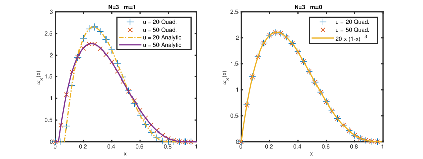
Figure 1: The single-particle longitudinal momentum fraction distribution from the light front parton gas model with $3$ partons. On the left panel, the partons are massive, with the available thermal energy $u$ measured in the unit of $m^{2}$. The blue stars and red crosses correspond to quadratures of Eq. (30) at $u=20\,m^{2}$ and $u=50\,m^{2}$ respectively. The yellow dot-dashed line and the purple solid line are the results from the analytic expression given by Eq. (27) at the corresponding $u$. On the right panel, the partons are massless. Therefore the available thermal energy is the only scale. Discrete points are results from quadrature using Eq. (30) at $u=20$ and $50$. The $\omega_{x}$ obtained from quadrature are independent of $u$. They agree with the analytic result $20\,x(1-x)^{3}$ within numerical errors.

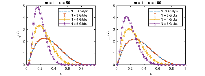
Figure 2: The single-particle longitudinal momentum fraction distribution from the massive light front parton gas model. The left panel shows results with $u=50\,m^{2}$. The right panel shows results with $u=100\,m^{2}$. The blue dot-dashed lines are the analytic results with $N=3$ using Eq. (27). The red, yellow, and purple points with error bars for the deviations correspond to the marginalization of the joint distribution in Eq. (21) using Gibbs sampling with $N=3,\,4$ and $5$ respectively. The means (points) and deviations (error bars) are calculated from $16$ independent samples for each combination of $N$ and $u$.

We then evaluate Eq. (30) with $N=3$ numerically using quadrature in the units where $m=1$. Since each kinematic term in the Hamiltonian given by Eq. (1) is positive definite, for any component of the transverse momentum being integrated we have a natural cutoff $\kappa_{j,\,x/y}<\max\{\sqrt{x_{j}u-m^{2}}\}=\sqrt{u-m^{2}}=\lambda$, where $\kappa_{j,\,x/y}$ stands for either the $x$- or the $y$-component of $\overrightarrow{\kappa}^{\perp}_{j}$. We sample transverse momentum components over the range from $-\lambda$ to $\lambda$ by the Simpson’s rule after the variable transform $\kappa_{j}=\lambda\,\mathrm{arctanh}\,(\phi_{j})$. For the numerical result to be accurate within $1\%$ from the analytic result, we allocate $99$ equally spaced quadrature points for each component of $\phi_{j}$ in the calculation with massive partons. While for massless partons, the same number is increased to $199$. The resulting $\omega_{x}$ at $u=20\,m^{2}$ and $u=50\,m^{2}$ are presented on the left panel of Fig. 1. For the massless partons, the numerical result for $\omega_{x}$ is shown on the right panel of Fig. 1. Both numerical results are in agreement with the analytic expressions given by Eqs. (26, 27). Therefore with quadrature in the specific case of $N=3$, we have tested the analytic reduction of the transverse integrals in Subsection 3.1. In the case of $N>3$, the support of $x_{j}$ integrals in Eq. (30) is specified by Eq. (31). For massive partons, the point $x_{j}=0$ is cut off by the energy delta function in Eq. (10). For massless partons, the point $x_{j}=0$ is singular, but measures zero after integration.

3.4 Gibbs sampling

With more than $3$ massive partons, we do not have an analytic expression for the single-particle distribution $\omega_{x}(x)$. Instead, we apply Markov Chain Monte Carlo algorithm to draw discretized samples of the joint distribution $\omega(E,V,N,\mathbf{P};\mathbf{x})$ given by Eq. (21). Because the number of independent momentum fractions in Eq. (21) is $N-1$, each sample of the joint distribution is represented by a $(N-1)$-dimensional random vector $x_{j}^{\lambda}$. Here the subscript $j\in\{1,\,2,\,\dots,\,N-1\}$ represents the vector index. While the sample point index is denoted by the superscript $\lambda\in\{1,\,2,\,\dots,\,S\}$, with $S$ being the sample size.

We apply the multi-stage Gibbs sampling to obtain samples of the joint distribution in Eq. (21), where one stochastic step only generates one component of the random vector [39]. Specifically for each update of the variable $x^{\lambda}_{j}$, we apply the Metropolis-Hastings algorithm with the acceptance probability given by

$$\rho_{\mathrm{MH}}(x_{j}^{\lambda},X_{j}^{\lambda+1})=\min\bigg{\{}1,\,\dfrac{f(X_{j}^{\lambda+1})}{f(x_{j}^{\lambda})}\dfrac{q(x_{j}^{\lambda}|X_{j}^{\lambda+1})}{q(X_{j}^{\lambda+1}|x_{j}^{\lambda})}\bigg{\}},$$ (32)

where the objective density $f$ is specified by the conditional distribution

$$\quad f(x_{j}^{\lambda}|x_{1}^{\lambda+1},x_{2}^{\lambda+1},\dots,x_{j-1}^{\lambda+1},x_{j+1}^{\lambda},\dots,x_{N-1}^{\lambda})$$

$$\propto\omega(E,V,N,\mathbf{P};x_{1}^{\lambda+1},x_{2}^{\lambda+1},\dots,x_{j-1}^{\lambda+1},x_{j}^{\lambda},x_{j+1}^{\lambda},\dots,x_{N-1}^{\lambda},x_{N})$$ (33)

with $x_{N}=1-\left(x_{1}^{\lambda+1}+x_{2}^{\lambda+1}+\dots+x_{j-1}^{\lambda+1}+x_{j}^{\lambda}+x_{j+1}^{\lambda}+\dots+x_{N-1}^{\lambda}\right)$. The function $\omega$ is given by Eq. (21) with the delta function factored out. The instrumental probability distribution $q(x|y)$ is the normal distribution with zero mean and an adjustable variance $a$:

$$q(x|y)=\dfrac{1}{\sqrt{2\pi a^{2}}}\exp\left[-\dfrac{(x-y)^{2}}{2a^{2}}\right].$$ (34)

Since $\rho(x|y)$ given by Eq. (34) is symmetric with respect to $x\leftrightarrow y$, Eq. (32) is simplified into $\rho_{\mathrm{MH}}(x_{j}^{\lambda},X_{j}^{\lambda+1})=\min\big{\{}1,\,f(X_{j}^{\lambda+1})/f(x_{j}^{\lambda})\big{\}}$. We then assign $x_{j}^{\lambda+1}=X_{j}^{\lambda+1}$ with probability of $\rho_{\mathrm{MH}}(x_{j}^{\lambda},X_{j}^{\lambda+1})$. Otherwise $x_{j}^{\lambda+1}=x_{j}^{\lambda}$. Such a procedure is repeated from $j=1$ to $j=N-1$ in order to produce one sample point for the random vector $x_{j}$.

For each sample, we choose $a=0.1$ and reach a sample size of $10^{6}$, after discarding the first $10^{5}$ sample points. The single-particle distribution $\omega_{x}(x)$ is obtained by directly binning and normalizing the sample with respect to a specific $x_{j}$. We then calculate the means and standard deviations of each bin in $\omega_{x}(x)$ as a histogram from $16$ independent samples. After normalization, the results are shown in Fig. 2. For $N=3$, they are in agreement with the analytic expression in Eq. (27). With fixed thermal energy, the distribution is shifted toward smaller $x$ with larger $N$. This is understood as $x_{j}=1/N$ is the most probable fraction in the joint $x$-distribution. The mean momentum fraction carried by a single parton is also $1/N$, which could be verified through $\int_{0}^{1}dx\,x\,\omega_{x}(E,V,N,\mathbf{P},x)=1/N$. With fixed $N$, the distribution becomes broader with higher thermal energy, as the support of the joint $x$-distribution increases.

4 Summary and conclusion

In this article, we proposed the light front parton gas model as a framework to help understand the distribution of the longitudinal momentum fractions of the partons inside a hadron based on light front kinematics and momentum conservation. Specifically within our model, the partons were treated as classical particles whose phase space distributions were given by the light front generalization of the microcanonical molecular dynamics ensemble.

We defined the longitudinal momentum fraction distributions as the marginalization of the phase space distribution. We also derived the joint longitudinal momentum fraction distribution through the analytic reduction of the transverse momentum integrals. This resulted in the explicit expressions of of the single-particle $x$-distribution for massless partons and $N=3$ massive partons. With specific choices of the parton number and available thermal energy, we calculated the single-particle momentum fraction distribution using quadrature. With Gibbs sampling, we drew samples of the joint longitudinal momentum fraction distribution for massive partons. Based on these samples, we computed the $\omega_{x}(E,V,N,\mathbf{P};x)$ as histograms for $N=3,\,4$ and $5$.

This article serves as the initial investigation of a light front parton gas model. Therefore we did not relate results presented in this article with experimental hadron PDFs. In future work, we expect to expand the current model to include spin and flavor to form a mixed system of massive quarks and massless gluons. We also plan to allow parton creation and annihilation that convert between quark-antiquark pairs and gluons, resulting in a microcanonical ensemble with variable particle numbers.

References

- [1] A. M. Cooper-Sarkar, R. C. E. Devenish, and A. De Roeck, “Structure functions of the nucleon and their interpretation,” Int. J. Mod. Phys. A13 (1998) 3385–3586, arXiv:hep-ph/9712301 [hep-ph].
- [2] A. Accardi, L. T. Brady, W. Melnitchouk, J. F. Owens, and N. Sato, “Constraints on large- parton distributions from new weak boson production and deep-inelastic scattering data,” Phys. Rev. D93 no. 11, (2016) 114017, arXiv:1602.03154 [hep-ph].
- [3] NNPDF Collaboration, R. D. Ball et al., “Parton distributions from high-precision collider data,” Eur. Phys. J. C77 no. 10, (2017) 663, arXiv:1706.00428 [hep-ph].
- [4] P. C. Barry, N. Sato, W. Melnitchouk, and C.-R. Ji, “First Monte Carlo Global QCD Analysis of Pion Parton Distributions,” Phys. Rev. Lett. 121 no. 15, (2018) 152001, arXiv:1804.01965 [hep-ph].
- [5] Y. L. Dokshitzer, “Calculation of the Structure Functions for Deep Inelastic Scattering and e+ e- Annihilation by Perturbation Theory in Quantum Chromodynamics.,” Sov. Phys. JETP 46 (1977) 641–653. [Zh. Eksp. Teor. Fiz.73,1216(1977)].
- [6] V. N. Gribov and L. N. Lipatov, “Deep inelastic e p scattering in perturbation theory,” Sov. J. Nucl. Phys. 15 (1972) 438–450. [Yad. Fiz.15,781(1972)].
- [7] G. Altarelli and G. Parisi, “Asymptotic Freedom in Parton Language,” Nucl. Phys. B126 (1977) 298–318.
- [8] F. M. Steffens and A. W. Thomas, “A Study of quark / parton distributions in a simple quark model,” Nucl. Phys. A568 (1994) 798–808.
- [9] F. M. Steffens and A. W. Thomas, “A Study of structure functions for the bag beyond leading order,” Prog. Theor. Phys. Suppl. 120 (1995) 145–156, arXiv:hep-ph/9509244 [hep-ph].
- [10] D. Diakonov, V. Petrov, P. Pobylitsa, M. V. Polyakov, and C. Weiss, “Nucleon parton distributions at low normalization point in the large N(c) limit,” Nucl. Phys. B480 (1996) 341–380, arXiv:hep-ph/9606314 [hep-ph].
- [11] D. Diakonov, V. Yu. Petrov, P. V. Pobylitsa, M. V. Polyakov, and C. Weiss, “Unpolarized and polarized quark distributions in the large N(c) limit,” Phys. Rev. D56 (1997) 4069–4083, arXiv:hep-ph/9703420 [hep-ph].
- [12] L. Mankiewicz and T. Weigl, “Physically motivated approximation to a parton distribution function in QCD,” Phys. Lett. B380 (1996) 134–140, arXiv:hep-ph/9604382 [hep-ph].
- [13] T. Weigl and L. Mankiewicz, “Combining lattice QCD results with Regge phenomenology in a description of quark distribution functions,” Phys. Lett. B389 (1996) 334–340, arXiv:hep-ph/9610205 [hep-ph].
- [14] W. Detmold, W. Melnitchouk, and A. W. Thomas, “Parton distributions from lattice QCD,” Eur. Phys. J.direct 3 no. 1, (2001) 13, arXiv:hep-lat/0108002 [hep-lat].
- [15] J.-W. Chen, L. Jin, H.-W. Lin, A. Schäfer, P. Sun, Y.-B. Yang, J.-H. Zhang, R. Zhang, and Y. Zhao, “Kaon Distribution Amplitude from Lattice QCD and the Flavor SU(3) Symmetry,” arXiv:1712.10025 [hep-ph].
- [16] K. Orginos, A. Radyushkin, J. Karpie, and S. Zafeiropoulos, “Lattice QCD exploration of parton pseudo-distribution functions,” Phys. Rev. D96 no. 9, (2017) 094503, arXiv:1706.05373 [hep-ph].
- [17] J.-W. Chen, L. Jin, H.-W. Lin, Y.-S. Liu, Y.-B. Yang, J.-H. Zhang, and Y. Zhao, “Lattice Calculation of Parton Distribution Function from LaMET at Physical Pion Mass with Large Nucleon Momentum,” arXiv:1803.04393 [hep-lat].
- [18] H.-W. Lin, J.-W. Chen, L. Jin, Y.-S. Liu, Y.-B. Yang, J.-H. Zhang, and Y. Zhao, “Spin-Dependent Parton Distribution Function with Large Momentum at Physical Pion Mass,” arXiv:1807.07431 [hep-lat].
- [19] Y.-S. Liu, J.-W. Chen, L. Jin, H.-W. Lin, Y.-B. Yang, J.-H. Zhang, and Y. Zhao, “Unpolarized quark distribution from lattice QCD: A systematic analysis of renormalization and matching,” arXiv:1807.06566 [hep-lat].
- [20] T. Izubuchi, X. Ji, L. Jin, I. W. Stewart, and Y. Zhao, “Factorization Theorem Relating Euclidean and Light-Cone Parton Distributions,” Phys. Rev. D98 no. 5, (2018) 056004, arXiv:1801.03917 [hep-ph].
- [21] G. Mangano, G. Miele, and G. Migliore, “Quantum statistics and Altarelli-Parisi evolution equations,” Nuovo Cim. A108 (1995) 867–882, arXiv:hep-ph/9510430 [hep-ph].
- [22] R. S. Bhalerao, “Statistical model for the nucleon structure functions,” Phys. Lett. B380 no. 1-2, (1996) 1–6, arXiv:hep-ph/9607315 [hep-ph]. [Erratum: Phys. Lett.B387,no.4,881(1996)].
- [23] C. Bourrely, J. Soffer, and F. Buccella, “A Statistical approach for polarized parton distributions,” Eur. Phys. J. C23 (2002) 487–501, arXiv:hep-ph/0109160 [hep-ph].
- [24] C. Bourrely and J. Soffer, “New developments in the statistical approach of parton distributions: tests and predictions up to LHC energies,” Nucl. Phys. A941 (2015) 307–334, arXiv:1502.02517 [hep-ph].
- [25] C. Bourrely and J. Soffer, “Statistical approach of pion parton distributions from Drell-Yan process,” ArXiv e-prints (Feb., 2018) , arXiv:1802.03153 [hep-ph].
- [26] S. J. Brodsky, H.-C. Pauli, and S. S. Pinsky, “Quantum chromodynamics and other field theories on the light cone,” Phys. Rept. 301 (1998) 299–486, arXiv:hep-ph/9705477 [hep-ph].
- [27] S. J. Brodsky, P. Hoyer, C. Peterson, and N. Sakai, “The Intrinsic Charm of the Proton,” Phys. Lett. 93B (1980) 451–455.
- [28] S. J. Brodsky, C. Peterson, and N. Sakai, “Intrinsic Heavy Quark States,” Phys. Rev. D23 (1981) 2745.
- [29] J. P. Vary, H. Honkanen, J. Li, P. Maris, S. J. Brodsky, A. Harindranath, G. F. de Teramond, P. Sternberg, E. G. Ng, and C. Yang, “Hamiltonian light-front field theory in a basis function approach,” Phys. Rev. C81 (2010) 035205, arXiv:0905.1411 [nucl-th].
- [30] Y. Li, P. Maris, X. Zhao, and J. P. Vary, “Heavy Quarkonium in a Holographic Basis,” Phys. Lett. B758 (2016) 118–124, arXiv:1509.07212 [hep-ph].
- [31] Y. Li, P. Maris, and J. P. Vary, “Quarkonium as a relativistic bound state on the light front,” Phys. Rev. D96 no. 1, (2017) 016022, arXiv:1704.06968 [hep-ph].
- [32] S. Tang, Y. Li, P. Maris, and J. P. Vary, “ mesons and their properties on the light front,” arXiv:1810.05971 [nucl-th].
- [33] S. Jia and J. P. Vary, “Basis light front quantization for the charged light mesons with color singlet Nambu-Jona-Lasinio interactions,” arXiv:1811.08512 [nucl-th].
- [34] J. P. Vary et al., “Hadron Spectra, Decays and Scattering Properties Within Basis Light Front Quantization,” Few Body Syst. 59 no. 4, (2018) 56, arXiv:1804.07865 [nucl-th].
- [35] J. E. Moyal, “Quantum mechanics as a statistical theory,” Proc. Cambridge Phil. Soc. 45 (1949) 99–124.
- [36] A. V. Belitsky and A. V. Radyushkin, “Unraveling hadron structure with generalized parton distributions,” Phys. Rept. 418 (2005) 1–387, arXiv:hep-ph/0504030 [hep-ph].
- [37] F. Lado, “Some topics in the molecular dynamics ensemble,” The Journal of Chemical Physics 75 no. 11, (1981) 5461–5463, https://doi.org/10.1063/1.441948.
- [38] F. Román, A. González, J. White, and S. Velasco, “On the calculation of the single-particle momentum and energy distributions for a hard-core fluid in the microcanonical molecular dynamics ensemble,” Physica A: Statistical Mechanics and its Applications 234 no. 1, (1996) 53 – 75.
- [39] C. Robert and G. Casella, Monte Carlo Statistical Methods. Springer texts in statistics. Springer, 1999.
- [40] J. Raufeisen and S. J. Brodsky, “Statistical physics and light-front quantization,” Phys. Rev. D70 (2004) 085017, arXiv:hep-th/0408108 [hep-th].
- [41] M. Beyer, S. Mattiello, T. Frederico, and H. J. Weber, “Light-front field theory of quark matter at finite temperature in the Nambu-Jona-Lasinio model,” J. Phys. G31 (2005) 21–27.
- [42] S. Strauss and M. Beyer, “Light front QED(1+1) at finite temperature,” Phys. Rev. Lett. 101 (2008) 100402, arXiv:0805.3147 [hep-th].
- [43] J. Raufeisen and S. J. Brodsky, “Finite-temperature field theory on the light front,” Few Body Syst. 36 (2005) 225–230, arXiv:hep-th/0409157 [hep-th].
- [44] J. Raufeisen, “Statistical physics on the light-front,” AIP Conf. Proc. 775 (2005) 202–211. [,202(2005)].
- [45] X.-d. Ji, J.-p. Ma, and F. Yuan, “QCD factorization for semi-inclusive deep-inelastic scattering at low transverse momentum,” Phys. Rev. D71 (2005) 034005, arXiv:hep-ph/0404183 [hep-ph].
- [46] B. Blok and M. Strikman, “Multiparton pp and pA Collisions: From Geometry to Parton–Parton Correlations,” Adv. Ser. Direct. High Energy Phys. 29 (2018) 63–99, arXiv:1709.00334 [hep-ph].
- [47] J. Jalilian-Marian, A. Kovner, L. D. McLerran, and H. Weigert, “The Intrinsic glue distribution at very small x,” Phys. Rev. D55 (1997) 5414–5428, arXiv:hep-ph/9606337 [hep-ph].
- [48] K. J. Golec-Biernat and M. Wusthoff, “Saturation effects in deep inelastic scattering at low Q**2 and its implications on diffraction,” Phys. Rev. D59 (1998) 014017, arXiv:hep-ph/9807513 [hep-ph].
- [49] K. J. Golec-Biernat and M. Wusthoff, “Saturation in diffractive deep inelastic scattering,” Phys. Rev. D60 (1999) 114023, arXiv:hep-ph/9903358 [hep-ph].
- [50] F. Gelis, E. Iancu, J. Jalilian-Marian, and R. Venugopalan, “The Color Glass Condensate,” Ann. Rev. Nucl. Part. Sci. 60 (2010) 463–489, arXiv:1002.0333 [hep-ph].