Constraining Non-local Gravity by S2 star orbits

Abstract

Non-local theories of gravity have recently gained a lot of interest because they can suitably represent the behavior of gravitational interaction in the ultraviolet regime. Furthermore, at infrared scales, they give rise to notable cosmological effects which could be important to describe the dark energy behavior. In particular, exponential forms of the distortion function seem particularly useful for this purpose. Using Noether Symmetries, it can be shown that the only non-trivial form of the distortion function is the exponential one, which is working not only for cosmological mini-superspaces, but also in a spherically symmetric spacetime. Taking this result into account, we study the weak field approximation of this type of non-local gravity, and comparing with the orbits of S2 star around the Galactic center (NTT/VLT data), we set constraints on the parameters of the theory. Non-local effects do not play a significant role on the orbits of S2 stars around Sgr A*, but give richer phenomenology at cosmological scales than the $\Lambda$CDM model. Also, we show that non-local gravity model gives better agreement between theory and astronomical observations than Keplerian orbits.

I Introduction

It is well established that General Relativity (GR), together with the associated concordance model in cosmology, $\Lambda$CDM, are the most successful explanations for gravitational and cosmological effects in the Universe. They have both passed the observational tests with flying colors. Cosmic Microwave Background Radiation, supernovae type Ia, large scale structures, as well as Solar System experiments and galactic rotation curves are some of these tests. However, the inability to find a convincing explanation for the accelerated expansion of the Universe, the huge discrepancy between the theoretical and observed values of the cosmological constant at early and late times, the fact that no particle candidate for dark matter has been observed at fundamental scales, together with the failure to confirm the existence of supersymmetry at TeV scales, led the scientists to pursue alternative explanations for the gravitational interaction.

The list of modifications is huge; from adding new fields, e.g. scalar-tensor, galileons, Kinetic Gravity Braiding (KGB), quintessence, Tensor-vector-scalar gravity (TeVeS), massive gravity, bi-gravity and more, to higher-order theories, e.g. $f(R)$, $f(\mathcal{G})$, conformal gravity, to higher dimensional theories, e.g. Kaluza-Klein, Dvali-Gabadadze-Porrati (DGP), Randal-Sundrum, as well as to emergent approaches, such as Causal Dynamical Triangulation (CDT) or entropic gravity. For more details, the interested reader is refereed to the exhausting literature Curvature ; capo11a ; clif12 ; Nojiri:2010wj ; Nojiri:2017ncd .

Among all the above, more than a decade ago, a non-local modification at infrared scales was proposed Deser:2007jk to explain the late-time acceleration of the universe. Non-localities usually appear naturally in quantum loop corrections, as well as when one considers the effective action approach to sting/M-theory. It has also been proposed Donoghue:1994dn ; Giddings:2006sj that such terms could be considered as solution to the black hole information paradox.

During this decade many attempts have been done in the literature to study non-localities in various contexts univ4 ; modesto1 ; modesto2 ; st1 ; st2 ; loop ; jm . Bouncing solutions in the string theory framework are discussed in Arefeva:2007wvo , while in Arefeva:2007xdy they present phantom dark energy solutions to explain the accelerated expansion of the Universe. Non-Gaussianities during inflation are studied in Barnaby:2008fk . Apart from the ultraviolet scales, a lot of progress has been done in the infrared scales too. Unification of inflation with late-time acceleration, as well as, the dynamics of a local form of the theory have been studied in Nojiri:2007uq ; Jhingan:2008ym . In Deser:2013uya , they prove that non-local gravities are ghost-free and stable and that they do not alter the predictions of GR for gravitationally bound systems. Last but not least, in Deffayet:2009ca , they try to fix the functional form of the distortion function, while in Koivisto:2008dh ; Koivisto:2008xfa they study the dynamics of the theory and its Newtonian limit. For a detailed review on the topic, we refer to Barvinsky:2014lja .

In parallel, symmetries always played a significant role in field theories. It would be thus very desired, if not necessary, if any new proposed theory is invariant under specific transformations. It has been proposed Cimento ; Gaetano ; Sergey ; Dialektopoulos:2018qoe ; Tsamparlis:2018nyo , that the Noether Symmetry Approach could be used as a selective criterion for gravitational models that are invariant under point transformations. It has been successfully studied in the literature numerous times Bahamonde:2017sdo ; Capozziello:2016eaz ; Capozziello:2018gms ; Bahamonde:2018zcq ; Bahamonde:2018ibz ; Karpathopoulos:2017ebb ; Paliathanasis:2017kzv ; Dimakis:2017kwx ; Paliathanasis:2014iva ; Basilakos:2013rua . It turns out that, apart from selecting theories of gravity, Noether symmetries of dynamical systems can help us calculate the invariant functions and use them to reduce the dynamics of the system and find analytical solutions.

In this paper, we consider the non-local theory proposed by Deser and Woodard but in its local representation. We apply the Noether Symmetry Approach in a spherically symmetric spacetime and find those functional forms of the distortion function, that keep the point-like Lagrangian invariant. Similar analysis in the cosmological minisuperspace Bahamonde:2017sdo has shown that the only possible forms are the linear and the exponential ones. The results included here are in complete agreement with those in cosmology. The linear form has been suggested Wetterich:1997bz to cure the unboundedness of the Euclidean gravity action, while the exponential Nojiri:2017ncd to explain the late-time acceleration, to unify the inflation era with the current one and more. However, up to now, they were both chosen by hand to explain phenomenology, while in Bahamonde:2017sdo and also here, the form of the non-local modification is chosen from first principles, that is the existence of the Noether symmetry.

Furthermore, we find the weak field limit of the theory with the exponential coupling and we also calculate the Post-Newtonian (PN) terms up to $g_{00}\sim\mathcal{O}(6)$. The local representation of this non-local model can be formulated as a biscalar-tensor theory. However, one of the two scalar fields is not dynamical. In the PN analysis, two new length scales arise, however, only one of them is physical; the other one belongs to the auxiliary degree of freedom introduced to localize the original action.

Finally, we consider the orbits of S2 star around the Galactic center and, by comparing the PN terms of our theory with observations, we are able to set some bounds on the above dynamical length scale. S-stars are the bright stars which move around the centre of our Galaxy ghez00 ; scho02 ; ghez08 ; gill09a ; gill09b ; genz10 ; gill12 ; meye12 ; gill17 ; hees17 ; chu17 where the compact radio source Sagittarius A* (or Sgr A*) is located. For one of them, called S2, a deviation from its Keplerian orbit was observed gill09a ; meye12 ; gill17 ; boeh17 ; hees17 ; chu17 , but the community debates to integrate its motion in the framework of GR.

Obviously, the non-localities are not expected to contribute significantly at astrophysical and galactic scales, because otherwise they would have been observed. However, what we see is that our approach is consistent with the orbits of S2 star around Sgr A* and thus we extend its range of validity, which up to now was only at cosmological scales, to the astrophysical ones too.

The present paper is organized as follows: in Sec. II we sketch the theory of non-local gravity and it biscalar-tensor representation. In Sec. III we apply the Noether Symmetry Approach in a spherically symmetric spacetime and we find those theories that are invariant under point transformations. In Sec. IV we derive weak field limit of the exponential coupling, as well as Post-Newtonian corrections. In Sec. V we describe the simulations of stellar orbits in the gravitational potential and the fitting procedure. An extended discussion about our results, together with future perspectives are presented in Sec. VI. We draw conclusions in Sec. VII.

II Non-local Gravity

It has been more than a decade that Deser and Woodard Deser:2007jk proposed a non-local modification of the Einstein-Hilbert action, which has the following form

$$\mathcal{S}=\frac{1}{2\kappa^{2}}\int d^{4}x\sqrt{-g}\left[R\left(1+f(\square^{-1}R)\right)\right]\,,$$ (1)

where $R$ is the Ricci scalar and $f(\square^{-1}R)$ is an arbitrary function, called distortion function, of the non-local term $\square^{-1}R$, which is explicitly given by the retarder Green’s function

$$\mathcal{G}[f](x)=(\square^{-1}f)(x)=\int d^{4}x^{\prime}\sqrt{-g(x^{\prime})}f(x^{\prime})G(x,x^{\prime})\,.$$ (2)

Setting $f(\square^{-1}R)=0$, the above action is equivalent to the Einstein-Hilbert one. The non-locality is introduced by the inverse of the d’Alembert operator.

A local representation of (1) has been proposed in Nojiri:2007uq ; they introduce two auxiliary scalar fields $\phi$ and $\xi$ and they rewrite the action (1) as

$$\mathcal{S} =\frac{1}{2\kappa^{2}}\int d^{4}x\sqrt{-g}\left[R\left(1+f(\phi)\right)+\xi\left(\square\phi-R\right)\right]$$

$$=\frac{1}{2\kappa^{2}}\int d^{4}x\sqrt{-g}\left[R\left(1+f(\phi)-\xi\right)-\nabla^{\alpha}\xi\nabla_{\alpha}\phi\right]\,,$$ (3)

where we just integrated out a total derivative. By varying the action with respect to $\xi$ and $\phi$ respectively, we get

$$\square\phi =R\Rightarrow\phi=\square^{-1}R\,,$$ (4)

$$\square\xi =-R\frac{df}{d\phi}\,,$$ (5)

where the equation (4) is just a constraint to recover (1), but the equation (5) is a non-trivial dynamical equation for $\xi$. Moreover, variation of the action (3) with respect to the metric yields,

$$\Big{(}1 +f(\phi)-\xi\Big{)}G_{\mu\nu}+\frac{1}{2}g_{\mu\nu}\nabla^{\alpha}\xi\nabla_{\alpha}\phi=$$

$$= \kappa^{2}T_{\mu\nu}^{M}+\nabla_{\mu}\xi\nabla_{\nu}\phi+\left(\nabla_{\mu}\nabla_{\nu}-g_{\mu\nu}\square\right)\left(f(\phi)-\xi\right)\,.$$ (6)

Another interesting equation is the trace of (6) which, after the use of (4),(5), reads

$$\left(1+f(\phi)-\xi-6f^{\prime}(\phi)\right) R=$$

$$=-\kappa^{2}T^{M}+\nabla_{\alpha}\xi\nabla^{\alpha}\phi +3f^{\prime\prime}(\phi)\nabla_{\alpha}\phi\nabla^{\alpha}\phi\,.$$ (7)

In the next section, we will use the Noether Symmetry Approach to select the form of the theory, i.e. the distortion function, in order for it to be invariant under point transformations. As we will see only the linear and the exponential forms will survive; the only ones that were interesting in the literature up to now.

III Noether Symmetries in Non-local gravity

Noether symmetries of second order differential equations can be connected to the collinations of the underlying manifold where the motion occurs. Thus, they can be used as a geometric criterion to determine the symmetries of dynamical systems, find the associated invariant functions and use them to reduce the dynamics of the system in order to find exact solutions.

The Noether Symmetry Approach Cimento has been extensively used in the literature to study the symmetries of several modified theories of gravity. The method goes as follows: we select a symmetry for the background spacetime which, in our case, is spherically symmetric. The metric is given by the following line element

$$ds^{2}=e^{\nu(t,r)}dt^{2}-e^{\lambda(t,r)}dr^{2}-r^{2}d\Omega^{2}\,,$$ (8)

where $\nu(t,r)$ and $\lambda(t,r)$ are two arbitrary function which depend both on time $t$ and the radial coordinate $r$, since we do not know a priori if Birkhoff’s theorem holds in non-local gravity.

Then, we substitute the metric (8) into the Lagrangian density (3) and after integrating out all the total derivative terms, we obtain the point-like Lagrangian which, here, reads

$$\mathcal{L}= e^{-\frac{1}{2}(\lambda+\nu)}\Big{(}-e^{\nu}r^{2}\nu_{r}\phi_{r}f^{\prime}(\phi)+e^{\lambda}r^{2}\lambda_{t}\phi_{t}f^{\prime}(\phi)-$$

$$-2e^{\nu}f(\phi)\left(e^{\lambda}+r\lambda_{r}-1\right)-2e^{\lambda+\nu}+2e^{\nu}+e^{\nu}r^{2}\xi_{r}\phi_{r}+$$

$$+e^{\nu}r^{2}\nu_{r}\xi_{r}-e^{\lambda}r^{2}\xi_{t}\phi_{t}-e^{\lambda}r^{2}\lambda_{t}\xi_{t}+$$

$$+2e^{\nu}\xi\left(e^{\lambda}+r\lambda_{r}-1\right)-2e^{\nu}r\lambda_{r}\Big{)}\,,$$ (9)

where the subscript denotes differentiation with respect to the variable.

The Noether vector, or else the generator of the point transformations, takes the form

$$X= \xi^{t}(t,r,\nu,\lambda,\phi,\xi)\partial_{t}+\xi^{r}(t,r,\nu,\lambda,\phi,\xi)\partial_{r}+$$

$$+\eta^{\nu}(t,r,\nu,\lambda,\phi,\xi)\partial_{\nu}+\eta^{\lambda}(t,r,\nu,\lambda,\phi,\xi)\partial_{\lambda}+$$

$$+\eta^{\phi}(t,r,\nu,\lambda,\phi,\xi)\partial_{\phi}+\eta^{\xi}(t,r,\nu,\lambda,\phi,\xi)\partial_{\xi}\,.$$ (10)

and in order for the dynamical system described by (9) to have symmetries the following condition Dialektopoulos:2018qoe has to be satisfied

$$X^{[1]}\mathcal{L}+\mathcal{L}\left(\frac{d\xi^{t}}{dt}+\frac{d\xi^{r}}{dr}\right)=\frac{dh^{t}}{dt}+\frac{dh^{r}}{dr}\,,$$ (11)

where $h^{t}$ and $h^{r}$ are two arbitrary functions depending on $(t,r,\nu,\lambda,\phi,\xi)$. Expanding the above condition, we find a system of 75 equations with 9 unknown variables, i.e. 6 coefficients of the Noether vector $\{\xi^{t},\,\xi^{r},\,\eta^{\nu},\,\eta^{\lambda},\,\eta^{\phi},\,\eta^{\xi}\}$, 2 unknown functions in the right hand side of (11), $\{h^{t},\,h^{r}\}$ and the form of the distortion function $f(\phi)$. Solving the system we find two possible models that are invariant under point transformations, that is

$$f(\phi)=c_{4}+c_{3}\phi,\,\,\,\text{and}\,\,\,f(\phi)=c_{4}+\frac{c_{5}}{c_{1}}e^{c_{1}\phi}\,.$$ (12)

Their symmetries are given by the following vectors respectively

$$X=\left(c_{1}t+\xi^{t}(r)\right)\partial_{t}-2c_{1}\partial_{\nu} +\left(c_{2}+2c_{1}\right)\partial_{\phi}+$$

$$+\left(c_{3}(c_{2}+2c_{1})\right)\partial_{\xi}\,,$$ (13)

$$X=\left(c_{2}t+\xi^{t}(r)\right)\partial_{t}-\frac{c_{3}}{2}r \partial_{r}-\left(2c_{2}+c_{3}\right)\partial_{\nu}+c_{1}c_{3}\partial_{\phi}+$$

$$+\left(c_{3}(\xi-c_{4}-1)\right)\partial_{\xi},$$ (14)

and in both cases, the functions in the right hand side of (11) are arbitrary functions of $(t,r)$. The associated invariant function of each symmetry is given by

$$I=\left(\xi^{t}+\xi^{r}\right)\left(\dot{q}^{i}\frac{\partial\mathcal{L}}{\partial\dot{q}^{i}}-\mathcal{L}\right)-\eta^{i}\frac{\partial\mathcal{L}}{\partial q^{i}}+h^{t}+h^{r}\,,$$ (15)

where $q$ are the variables of the configuration space, which, in our case, is $\mathcal{Q}=\{\nu,\lambda,\phi,\xi\}$.

For the sake of completeness we have to say that, from the Noether vectors (13) and (14), one can construct the following Lagrange system

$$\frac{dt}{\xi^{t}}=\frac{dr}{\xi^{r}}=\frac{d\nu}{\eta^{\nu}}=\frac{d\lambda}{\eta^{\lambda}}=\frac{d\phi}{\eta^{\phi}}=\frac{d\xi}{\eta^{\xi}}\,,$$ (16)

solve for each variable and find the so-called $0^{\text{th}}$ order invariants. Substituting these in the Euler-Lagrange equations given by (9), one can reduce the dynamics of the system and find exact spherically symmetric solutions. However, the point of this paper is to use the above forms of the distortion function and to study its weak field limit. This is what we are going to do in the following section.

IV Weak field approximation

We consider the exponential form for the distortion function, given by (12), and we derive the non-local gravity potential in the weak field limit to test the orbit of the S2 star against it. Then, we compare the results with the set of S2 star orbit observations obtained by New Technology Telescope/Very Large Telescope (NTT/VLT). This study is a continuation of our previous studies where we considered various gravity models bork12 ; bork13 ; capo14 ; zakh14 ; bork16 ; bork16a ; capo17 ; zakh16 ; zakh18 .

It is well known from GR that, in order to recover the Newtonian potential for time-like particles we have to expand the $g_{00}$ component of the metric to $\Phi\sim\upsilon^{2}\sim\mathcal{O}(2)$, where $\Phi$ is the Newtonian potential and $\upsilon$ is the 3-velocity of a fluid element. If we want to study the PN limit we have to expand the components of the metric as

$$g_{00}\sim\mathcal{O}(6)\,,\,\,g_{0i}\sim\mathcal{O}(5)\,\,\text{and}\,\,g_{ij}\sim\mathcal{O}(4)\,.$$ (17)

Obviously, for the lowest order of the PN approximation we do not have to go up to $\mathcal{O}(6)$. However, as we would expect, two new length scales arise, which are related to the scalar degrees of freedom and thus we have to compute higher order corrections.

We want to study the behavior of the gravitational field generated by a point-like source and we consider that the metric is static and spherically symmetric. Before proceeding, it is worth to make the following comment; even though in principle, we do not expect that Birkhoff’s theorem is valid in non-local gravity, and that is the reason why, in order to derive the Noether symmetries, we considered a time-dependent line element, it is reasonable to believe that, as a first approximation in weak-field gravity, a static and spherically symmetric metric works as well. With this position, the metric assumes the form

$$ds^{2}=A(r)dt^{2}-B(r)dr^{2}-r^{2}d\Omega^{2}\,.$$ (18)

Although, we could take as fact that $B(r)=1/A(r)$, in alternative theories of gravity, this cannot be chosen a priori, since the existence of such solutions is not necessary.

Obviously, since the metric (18) depends only on the radial coordinate, the scalar fields inherit the isometries of the metric and thus we have $\phi=\phi(r)$ and $\xi=\xi(r)$. The expansion of the metric components, as well as the scalar fields, read

$$A(r) =1+\frac{1}{c^{2}}\Phi(r)^{(2)}+\frac{1}{c^{4}}\Phi(r)^{(4)}+\frac{1}{c^{6}}\Phi(r)^{(6)}+\mathcal{O}(8)\,,$$ (19a)

$$B(r) =1+\frac{1}{c^{2}}\Psi(r)^{(2)}+\frac{1}{c^{4}}\Psi(r)^{(4)}+\mathcal{O}(6)\,,$$ (19b)

$$\phi(r) =\phi_{0}+\frac{1}{c^{2}}\phi(r)^{(2)}+\frac{1}{c^{4}}\phi(r)^{(4)}+\frac{1}{c^{6}}\phi(r)^{(6)}+\mathcal{O}(8)\,,$$ (19c)

$$\xi(r) =\xi_{0}+\frac{1}{c^{2}}\xi(r)^{(2)}+\frac{1}{c^{4}}\xi(r)^{(4)}+\frac{1}{c^{6}}\xi(r)^{(6)}+\mathcal{O}(8)\,,$$ (19d)

where $\phi_{0}$ and $\xi_{0}$ are the constant background values of each field .

If we substitute the exponential form (12) for $f(\phi)$, i.e. $f=1+e^{\phi}$ , we get the following four equations: the $00-$ and $11-$ components of (6) and the two equations of the two scalar fields, (4) and (5) respectively

$$2B^{2}\left(-\xi+e^{\phi}+2\right)+rB^{\prime}\left(-2\xi-r\xi^{\prime}+re^{\phi}\phi^{\prime}+2e^{\phi}+4\right)-$$

$$-B\left(-2\xi+2\left(-r^{2}\xi^{\prime\prime}+r^{2}e^{\phi}\phi^{\prime\prime}+r^{2}e^{\phi}\left(\phi^{\prime}\right)^{2}+2re^{\phi}\phi^{\prime}+e^{\phi}+2\right)+r\xi^{\prime}\left(r\phi^{\prime}-4\right)\right)=0\,,$$ (20)

$$rA^{\prime}\left(-2\xi-r\xi^{\prime}+re^{\phi}\phi^{\prime}+2e^{\phi}+4\right)-$$

$$-A\left(2B\left(-\xi+e^{\phi}+2\right)+2\xi+r^{2}\xi^{\prime}\phi^{\prime}+4r\xi^{\prime}-4re^{\phi}\phi^{\prime}-2e^{\phi}-4\right)=0\,,$$ (21)

$$A^{2}\left(-4B^{2}e^{\phi}+rB^{\prime}\left(r\xi^{\prime}-4e^{\phi}\right)+B\left(-2r^{2}\xi^{\prime\prime}-4r\xi^{\prime}+4e^{\phi}\right)\right)+Br^{2}\left(-e^{\phi}\right)\left(A^{\prime}\right)^{2}+$$

$$+Ar\left(B\left(2re^{\phi}A^{\prime\prime}+A^{\prime}\left(4e^{\phi}-r\xi^{\prime}\right)\right)-re^{\phi}A^{\prime}B^{\prime}\right)=0\,,$$ (22)

$$A^{2}\left(-4B^{2}-rB^{\prime}\left(r\phi^{\prime}+4\right)+2B\left(r^{2}\phi^{\prime\prime}+2r\phi^{\prime}+2\right)\right)+B\left(-r^{2}\right)\left(A^{\prime}\right)^{2}+$$

$$+Ar\left(B\left(2rA^{\prime\prime}+A^{\prime}\left(r\phi^{\prime}+4\right)\right)-rA^{\prime}B^{\prime}\right)=0\,.$$ (23)

Plugging the perturbations (19a)-(19d) into the above Eqs. (IV)-(IV), we obtain three systems of four equations, one for each order, $\mathcal{O}(2),\,\mathcal{O}(4)$ and $\mathcal{O}(6)$. Since $B$ is calculated up to order $\mathcal{O}(4)$, in the last system, one of the equations will be a constraint to fix arbitrary integration constants. The solutions have the form

$$A(r)=1-\frac{2G_{N}M\phi_{c}}{c^{2}r}+\frac{G_{N}^{2}M^{2}}{c^{4}r^{2}}\left[\frac{14}{9}\phi_{c}^{2}+\frac{18r_{\xi}-11r_{\phi}}{6r_{\xi}r_{\phi}}r\right]-\frac{G_{N}^{3}M^{3}}{c^{6}r^{3}}\left[\frac{50r_{\xi}-7r_{\phi}}{12r_{\xi}r_{\phi}}\phi_{c}r+\frac{16\phi_{c}^{3}}{27}-\frac{r^{2}\left(2r_{\xi}^{2}-r_{\phi}^{2}\right)}{r_{\xi}^{2}r_{\phi}^{2}}\right]\,,$$ (24a)

$$B(r)=1+\frac{2G_{N}M\phi_{c}}{3c^{2}r}+\frac{G_{N}^{2}M^{2}}{c^{4}r^{2}}\left[\frac{2\phi_{c}^{2}}{9}+\left(\frac{3}{2r_{\xi}}-\frac{1}{r_{\phi}}\right)r\right]\,,$$ (24b)

$$\phi(r)=\frac{4G_{N}M\phi_{c}}{3c^{2}r}-\frac{G_{N}^{2}M^{2}}{c^{4}r^{2}}\left[\left(\frac{11}{6r_{\xi}}+\frac{1}{r_{\phi}}\right)r-\frac{2\phi_{c}^{2}}{9}\right]-\frac{G_{N}^{3}M^{3}}{c^{6}r^{3}}\left[\frac{r^{2}}{r_{\phi}^{2}}-\left(\frac{25}{12r_{\xi}}-\frac{7}{6r_{\phi}}\right)\phi_{c}r-\frac{4\phi_{c}^{3}}{81}\right]\,,$$ (24c)

$$\xi(r)=1+\frac{G_{N}^{2}M^{2}}{c^{4}r^{2}}\left[\frac{2\phi_{c}^{2}}{3}-\left(\frac{13}{6r_{\xi}}-\frac{1}{r_{\phi}}\right)r\right]+\frac{G_{N}^{3}M^{3}}{c^{6}r^{3}}\left[\frac{20\phi_{c}^{3}}{27}-\left(\frac{1}{r_{\xi}^{2}}-\frac{1}{r_{\phi}^{2}}\right)r^{2}-\left(\frac{131}{36r_{\xi}}+\frac{1}{6r_{\phi}}\right)\phi_{c}r\right]\,.$$ (24d)

Here $\phi_{c}$ is a dimensionless constant and thus the effective gravitational coupling is $G_{\text{eff}}=G_{N}\phi_{c}$. Moreover, we see that two new length scales arise in the $\mathcal{O}(4)$ order. These are related to the two scalar degrees of freedom, $\phi$ and $\xi$ and thus to the non-localities. They are denoted as $r_{\phi}$ and $r_{\xi}$ respectively.

V Simulated orbits of S2 star in Non-local gravity potential

In order to constrain the free parameters, $\phi_{c},\,r_{\phi}$ and $r_{\xi}$ we have to consider the orbit of S2 star around the Galactic centre and fit them to astronomic observations by NTT/VLT. To do this we will need from the previous results the gravitational potential of the $g_{00}$ component of the metric, i.e. $A(r)$, (24a). Following the expansion (19a), we identify

$$\Phi^{(2)}(r) =-\frac{2G_{N}M}{r}\phi_{c}\,,$$ (25)

$$\Phi^{(4)}(r) =\frac{G_{N}^{2}M^{2}}{r^{2}}\left[\frac{14}{9}\phi_{c}^{2}+\frac{18r_{\xi}-11r_{\phi}}{6r_{\xi}r_{\phi}}r\right]\,,$$ (26)

$$\Phi^{(6)}(r) =\frac{G_{N}^{3}M^{3}}{r^{3}}\left[\frac{7r_{\phi}-50r_{\xi}}{12r_{\xi}r_{\phi}}\phi_{c}r-\frac{16\phi_{c}^{3}}{27}+\frac{2r_{\xi}^{2}-r_{\phi}^{2}}{r_{\xi}^{2}r_{\phi}^{2}}r^{2}\right]$$ (27)

We want to determine the free parameters of the theory, $\phi_{c},\,r_{\phi}$ and $r_{\xi}$. We take specific values for $\phi_{c}$ = 1 (in order to obtain the Newtonian limit), and fix the parameter space of the other two.

Our aim is to determine these parameters using astrometric observations of S2 star orbit. In order to constrain parameters $r_{\phi}$ and $r_{\xi}$ by astronomical observations, we performed two-body simulations in non-local gravity potential

$$\mathbf{\dot{r}}=\mathbf{v},\hskip 14.22636pt\mu\mathbf{\ddot{r}}=-\triangledown{U_{NL}}\left(\mathbf{r}\right),$$ (28)

where $\mu={M\cdot m_{S}}/({M+m_{S}})$ is the reduced mass in the two-body problem.

The positions of the S2 star along its true orbit are calculated at the observed epochs using two-body simulations in the non-local gravity potential, assuming that distance to the S2 star is $d$ = 8.3 kpc and mass of central black hole $M_{BH}$=4.3 $\times 10^{6}M_{\odot}$ gill09b . In order to compare them with observed positions we have to calculate the corresponding apparent orbits ($x$, $y$) bork13 . The mass $M_{BH}$ of central object can be obtained independently using different observational techniques, such as e.g. virial analysis of the ionized gas in the central parsec lacy82 , $M-\sigma$ (mass - bulge velocity dispersion), the relationship for the Milky Way trem02 , or from orbits of S-stars gill09a ; gill09b . In the latter case, the mass of the SMBH was estimated using 2-body and N-body Keplerian and general relativistic orbit models (see gill17 ). Inspite the fact that relativistic 2-body models resulted with slightly bigger values for both $M_{BH}$ and $d$, it was not possible to obtain the stastistically significant difference between these estimates, nor to detect any of the leading-order relativistic effects gill17 . Similarly, it would be also the case with mass estimates obtained by our 2-body simulations in non-local gravity. Therefore, in our simulations we used the statistically most significant estimates obtained from combined Keplerian orbit fit of 17 S-stars, which were also in agreement with a corresponding results determined from the statistical cluster parallax (see gill17 ). Since our goal was not to make a new estimate of mass $M_{BH}$ using non-local gravity, but instead studying the possible deviations from Keplerian orbit of S2 star (which could indicate signatures for non-local gravity on these scales), we adopted the above estimates for the mass of central object ($M_{BH}=4.3\times 10^{6}M_{\odot}$), as well as the distance to the S2 star given by gill09a ; gill09b ($d$ = 8.3 kpc), and constrained only the remaining two free parameters of non-local gravity potential ($r_{\phi}$, $r_{\xi}$). One should also note that slightly different masses would effect the values of precession angle but not significantly.

We vary the parameters $r_{\phi}$ and $r_{\xi}$ over some intervals, and search for those solutions which for the simulated orbits in non-local gravity give at least the same ($\chi^{2}$ = 1.89) or better fits ($\chi^{2}<1.89$) than the Keplerian orbits.

We are simulating orbit of S2 star in the non-local gravity potential by numerical integration of equations of motion. We perform fitting using LMDIF1 routine from MINPACK-1 Fortran 77 library which solves the nonlinear least squares problems by a modification of Marquardt-Levenberg algorithm more80 ; bork13 , according to the following procedure:

1. We start the first iteration using a guess of initial position $(x_{0},y_{0})$ and velocity $(\dot{x}_{0},\dot{y}_{0})$ of S2 star in the orbital plane (true orbit) at the epoch of the first observation;

2. the true positions $(x_{i},y_{i})$ and velocities $(\dot{x}_{i},\dot{y}_{i})$ at all successive observed epochs are then calculated by numerical integration of equations of motion, and projected into the corresponding positions $(x_{i}^{c},y_{i}^{c})$ in the observed plane (apparent orbit);

3. in order to obtain discrepancy between the simulated and observed apparent orbit, we estimate the reduced $\chi^{2}$:

   $$\chi^{2}=\dfrac{1}{2N-\nu}{\sum\limits_{i=1}^{N}{\left[{{{\left({\dfrac{x_{i}^{o}-x_{i}^{c}}{\sigma_{xi}}}\right)}^{2}}+{{\left(\dfrac{y_{i}^{o}-y_{i}^{c}}{\sigma_{yi}}\right)}^{2}}}\right]}},$$ (29)

   where $(x_{i}^{o},y_{i}^{o})$ and $(x_{i}^{c},y_{i}^{c})$ are the corresponding observed and calculated apparent positions, $N$ is the number of observations, $\nu$ is number of initial conditions (in our case $\nu=4$), $\sigma_{xi}$ and $\sigma_{yi}$ are uncertainties of observed positions;

4. the new initial conditions are estimated by the fitting routine and the steps 2-3 are repeated until the fit is converging, i.e. until the minimum of reduced $\chi^{2}$ is achieved.

For more detailed description about fitting procedure and numerics see in papers more80 ; bork13 .

VI Results and Discussion

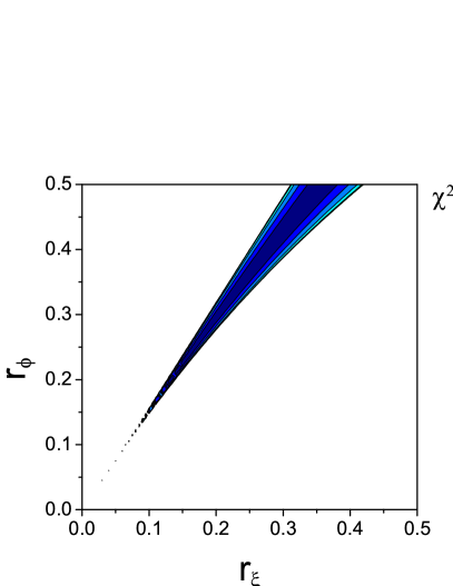
Figure 1: (Color online) The maps of the reduced $\chi^{2}$ over the $r_{\phi}-r_{\xi}$ parameter space (in $AU$) for all simulated orbits of S2 star which give at least the same or better fits than the Keplerian orbits ($\chi^{2}$ = 1.89). With a decreasing value of $\chi^{2}$ (better fit) colors in grey scale are darker. A few contours are presented for specific values of reduced $\chi^{2}$ given in the figure’s legend.

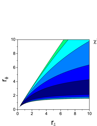
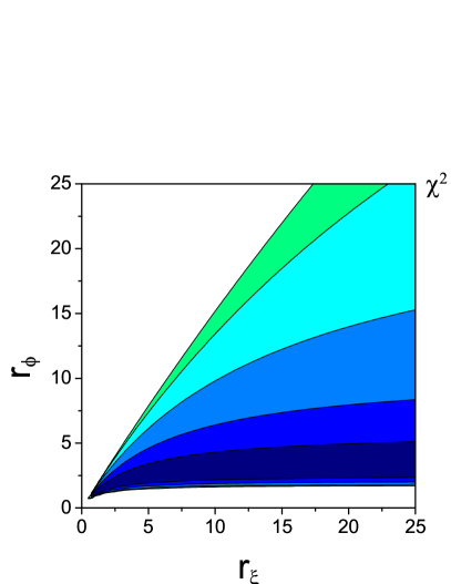
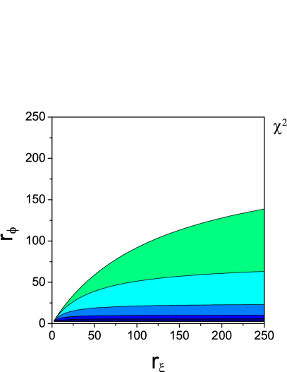
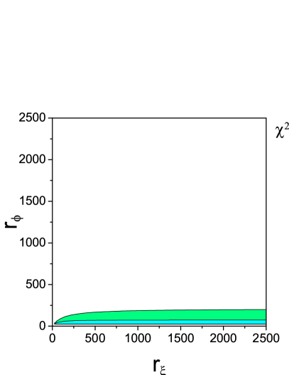
Figure 2: The same like figure 1, but for more extended region of $r_{\phi}-r_{\xi}$ parameter space.

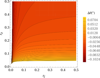
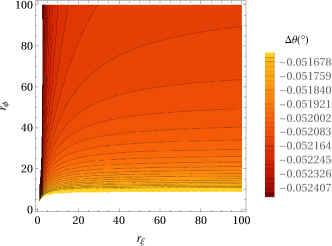
Figure 3: (Color online) The precession per orbital period for $r_{\phi}-r_{\xi}$ parameter space in the case of non-local modified gravity potential. With a decreasing value of angle of precession colors are darker.

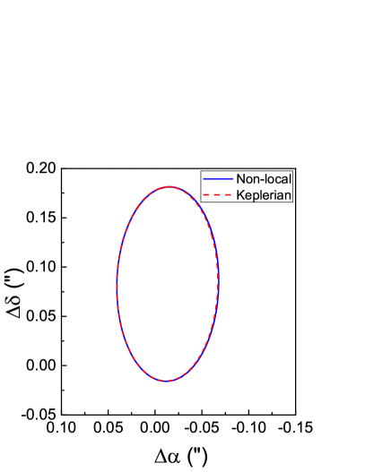
Figure 4: Comparisons between the orbit of S2 star in Newtonian gravity (red dashed line) and non-local gravity (blue solid line) in the observed plane, i.e. apparent orbit. Parameters of non-local gravity are $r_{\phi}$ = 1.2 AU and $r_{\xi}$ = 1.1 AU.

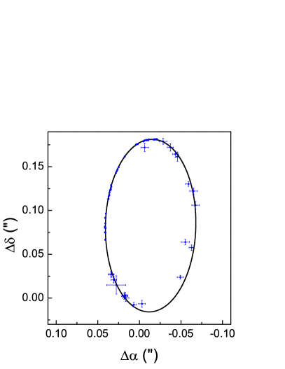
Figure 5: A fitted orbit in non-local gravity through the following (parameters $r_{\phi}$ = 1.2 AU and $r_{\xi}$ = 1.1 AU (($\chi^{2}$ = 1.72)) observations of S2 star (denoted by points with error bars) NTT/VLT (see figure 3 from gill09a ).

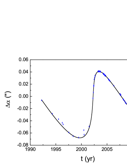
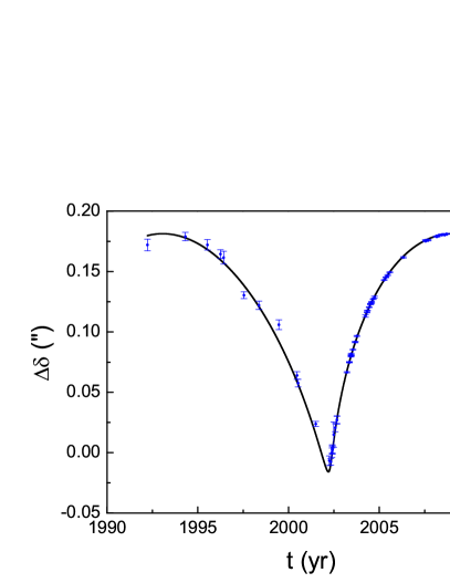
Figure 6: The comparisons between the observed (circles with error bars) and fitted (solid lines) coordinates of S2 star for $\Delta\alpha$ (left panel) and $\Delta\delta$ (right panel) in the case of NTT/VLT observations and non-local gravity potential (parameters $r_{\phi}$ = 1.2 AU and $r_{\xi}$ = 1.1 AU).

In Figs. 1 - 2 we presented the maps of the reduced $\chi^{2}$ over the $r_{\phi}-r_{\xi}$ parameter space for all simulated orbits of S2 star which give at least the same or better fits than the Keplerian orbits. The second term of the RHS in Eq. (27) has a inverse $r$ term, namely $r^{-2}\times r=r^{-1}$. This term can potentially make a large deviation from the Keplerian orbit. A point is that the coefficient of this term is proportional to $18r_{\xi}-11r_{\phi}$. Therefore, the (probably) dominant deviation vanishes (and the $\chi^{2}$ is thus small), if $r_{\phi}=(18/11)r_{\xi}$. This is exactly corresponding to the dark region (small $\chi^{2}$) in Figure 1. For more extended parameter space (see Figure 2), values of $\chi^{2}$ is almost nonsensitive on $r_{\xi}$ parameter.

As it can be seen from Fig. 1 - Fig. 2, the most probable value for the scale parameter $r_{\phi}$, in the case of NTT/VLT data set observations of S2 star, is $\approx$ 0.1 - 2.5 AU. Moreover, as we see it is not possible to obtain constraints for the second length scale, $r_{\xi}$. This is because this length scale is associated with one of the scalar fields which is not dynamical, but it only plays an auxiliary role to localize the original non-local Lagrangian. Thus, it is obvious that we cannot constrain it.

In order to calculate the orbital precession in non-local gravity, we assume that the weak field potential does not differ significantly from the Newtonian potential, i.e. the perturbing potential:

$$V(r)=U_{NL}-U_{N};\quad\text{ is small, where}\quad U_{N}=-\dfrac{GM}{r}.$$ (30)

The weak field potential of the non-local gravity reads

$$U_{NL}= -\frac{G_{N}M}{r}\phi_{c}\ +\frac{G_{N}^{2}M^{2}}{2c^{2}r^{2}}\left[\frac{14}{9}\phi_{c}^{2}+\frac{18r_{\xi}-11r_{\phi}}{6r_{\xi}r_{\phi}}r\right]$$

$$+\frac{G_{N}^{3}M^{3}}{2c^{4}r^{3}}\left[\frac{7r_{\phi}-50r_{\xi}}{12r_{\xi}r_{\phi}}\phi_{c}r-\frac{16\phi_{c}^{3}}{27}+\frac{2r_{\xi}^{2}-r_{\phi}^{2}}{r_{\xi}^{2}r_{\phi}^{2}}r^{2}\right]\,.$$ (31)

In Fig. 3 we presented precession per orbital period for $r_{\phi}-r_{\xi}$ parameter space in the case of non-local gravity potential. We can notice that for values $r_{\phi}$ less then about $\approx$ 0.2 AU precession is positive, and for bigger values is negative. We hope that future more precise astronomical data will help us to better constrain non-local gravity parameters.

The particular form of the chosen Lagrangian among the class of non-local theories of gravity induces the precession of S2 star orbit. Depending of the values of parameters in the $r_{\phi}-r_{\xi}$ parameter space, precession of S2 star orbit calculated in non-local gravity can have positive or negative sign, i.e. the same or the opposite direction with respect to GR. In both cases the pericenter shift per orbital revolution is on the same order of magnitude as in GR, which predicts that pericenter of S2 star should advance by $0^{\circ}.18$ per orbital revolution gill09b .

In Figs. 4-6, we use one of the values for best fit parameters: $r_{\phi}$ = 1.2 AU and $r_{\xi}$ = 1.1 AU. For this choice of best fit papameters the value $\chi^{2}$ = 1.72. From Figs. 1-2 it is obvious that there are infinity number of such parameters where agreement is better than in Keplerian case ($\chi^{2}$ = 1.89), i. e. it is not possible to obtain reliable constrains on the parameter $r_{\xi}$. From Fig. 3 (left panel) we can see that there are areas in the $r_{\phi}-r_{\xi}$ parameter space where precession of S2 star orbit calculated in non-local gravity can have positive or negative sign. In both cases of precession there are areas where agreement between non-local gravity and observation is better than in Keplerian case. It means that one can make even stringer constrains of parameters $r_{\phi}$ and $r_{\xi}$ by requiring that precession must has positive or negative direction (like in GR or oposite). However, current precision of astrometric observations is not precise enough to definitly resolve this issue, and thus we give our result without this constraint. We choose area in the $r_{\phi}-r_{\xi}$ parameter space where precession is negative (opposite of GR) because in that case agreement with observations is better($\chi^{2}$ = 1.72) than in case when precession is positive ($\chi^{2}$ = 1.78).

Comparison between the fitted orbit of S2 star in Newtonian gravity (red dashed line) and non-local gravity (blue solid line) in the observed plane is presented in Fig. 4. We can notice that difference between the orbit of S2 star in Keplerian case and in non-local gravity is very small.

In Fig. 5 the fitted orbit in non-local gravity through the NTT/VLT observations of S2 star (denoted by points with error bars) are presented. The comparisons between the observed (circles with error bars) and fitted (solid lines) $\Delta\alpha$ and $\Delta\delta$ coordinates of S2 star in the case of NTT/VLT observations and non-local gravity potential are given in Fig. 6. We can see that agreement between observed and fitted coordinates of S2 star is very good.

VII Conclusions

Non-local gravity theories are very well motivated from cosmology, since they give a good explanation in the late-time acceleration of the Universe, without invoking exotic forms of matter-energy. However, a theory of gravity should be valid at all scales and that is why we wanted to study such theories at smaller scales, i.e. astrophysical.

We considered a theory (1) proposed some years ago by Deser and Woodard [6], we “localized” it (3) as was proposed in [20] and we studied its invariance under point-transformations in a spherically symmetric spacetime. Surprisingly, we found that the forms of the distortion function that leave the action invariant are the same with those in a cosmological minisuperspace [31].

What we did next is, we selected the non-trivial form for the distortion function, i.e. the exponential $f(\phi)=1+e^{\phi}$, that reproduces also the correct cosmological dynamics and we studied its weak field limit. After verifying that an asymptotically flat background consists a solution to the theory (3) with constant scalar fields, we perturbed the Minkowski background to $1/c^{2}$ terms up to third order, i.e. (19a)-(19d). The solutions we found are the Eqs. (24a)-(24d) and as we see two new-length scales arose; one for each scalar field.

We would like to confront our results with reality and specifically to find constraints on the two new length scales. That is why, we compared our results with the orbits of S2 star around the Galactic Center. We obtained the values for $r_{\phi}$ and $r_{\xi}$ parameters showing that the S2 star orbit in non-local gravity fits better the astrometric data than Keplerian orbit. The most probable value for the scale parameter $r_{\phi}$ is approximately from 0.1 to 2.5 AU. It is not possible to obtain reliable constrains on the parameter $r_{\xi}$ of non-local gravity using only observed astrometric data for S2 star because this length scale is associated with one of the scalar fields which is not dynamical, but only plays an auxiliary role to localize the original non-local Lagrangian.

The precession of S2 star orbit in non-local gravity can have the same or the opposite direction with respect to GR, depending on the $r_{\phi}-r_{\xi}$ parameters, i.e. for values $r_{\phi}\lesssim 0.2$ AU, the precession is positive, and for bigger values is negative. The obtained orbital precession of the S2 star in non-local gravity is on the same order of magnitude as in GR; in the future, more precise astronomical data will help us better constrain the non-local gravity parameters. However, it is normal to believe that, non-local effects do not play a significant role at scales comparable to the S2 star orbit, i.e. astrophysical scales, but only at cosmological ones. There could be a screening effect, or a specific radius (maybe even given by the new length scale), after which non-local effects would start becoming significant.

The approach we are proposing can be used to constrain different modified gravity models from stellar orbits around Galactic centre (see also Ivan1 ; Ivan2 ; Ivan3 ; Ivan4 ; dela18 ).

- (1) S. Capozziello, Int. J. Mod. Phys. D 11 483 (2002).
- (2) S. Capozziello and M. de Laurentis, Phys. Rep. 509 167 (2011).
- (3) T. Clifton, P. G. Ferreira, A. Padilla, and C. Skordis, Phys. Rep. 513 1 (2012).
- (4) S. Nojiri and S. D. Odintsov, Phys. Rept. 505, 59 (2011).
- (5) S. Nojiri, S. D. Odintsov, and V. K. Oikonomou, Phys. Rept. 692, 1 (2017).
- (6) S. Deser and R. P. Woodard, Phys. Rev. Lett. 99, 111301 (2007).
- (7) J. F. Donoghue, Phys. Rev. D 50, 3874 (1994).
- (8) S. B. Giddings, Phys. Rev. D 74, 106005 (2006).
- (9) S. Das and E. C. Vagenas, Phys. Rev. Lett. 101, 221301 (2008).
- (10) L. Modesto and I.L. Shapiro, Phys. Lett. B 755, 279 (2016).
- (11) L. Modesto, Nucl. Phys. B 909, 584 (2016).
- (12) G. Calcagni and L. Modesto, J. Phys. A: Math. Theor. 47, 355402 (2014).
- (13) G. Calcagni and G. Nardelli, Phys. Rev. D 82, 123518 (2010).
- (14) S. A. Major and M. D. Seifert, Class. Quant. Grav. 19, 2211 (2002).
- (15) L. Modesto, J. W. Moffat and P. Nicolini, Phys. Lett. B 695, 397 (2011).
- (16) I. Y. Aref’eva, L. V. Joukovskaya, and S. Y. Vernov, JHEP 0707, 087 (2007).
- (17) I. Y. Aref’eva, L. V. Joukovskaya, and S. Y. Vernov, J. Phys. A 41, 304003 (2008).
- (18) N. Barnaby and J. M. Cline, J. Cosmol. Astropart. P. 0806, 030 (2008).
- (19) S. Jhingan, S. Nojiri, S. D. Odintsov, M. Sami, I. Thongkool, and S. Zerbini, Phys. Lett. B 663, 424 (2008).
- (20) S. Nojiri and S. D. Odintsov, Phys. Lett. B 659 821 (2008).
- (21) S. Deser and R. P. Woodard, J. Cosmol. Astropart. P. 1311, 036 (2013).
- (22) C. Deffayet and R. P. Woodard, J. Cosmol. Astropart. P. 0908, 023 (2009).
- (23) T. Koivisto, Phys. Rev. D 77, 123513 (2008).
- (24) T. S. Koivisto, Phys. Rev. D 78, 123505 (2008).
- (25) A. O. Barvinsky, Mod. Phys. Lett. A 30, no.03n04, 1540003 (2015).
- (26) S. Capozziello, R. De Ritis, C. Rubano and P. Scudellaro, Riv. Nuovo Cim. 19N4, 1 (1996).
- (27) S. Capozziello and G. Lambiase, Gen. Rel. Grav. 32, 673 (2000).
- (28) S. Capozziello, M. De Laurentis and S. D. Odintsov, Eur. Phys. J. C 72, 2068 (2012).
- (29) K. F. Dialektopoulos and S. Capozziello, Int. J. Geom. Meth. Mod. Phys. 15, no.supp01, 1840007 (2018).
- (30) M. Tsamparlis and A. Paliathanasis, Symmetry 10, no.7, 233 (2018).
- (31) S. Bahamonde, S. Capozziello, and K. F. Dialektopoulos, Eur. Phys. J. C 77, no.11, 722 (2017).
- (32) S. Capozziello, K. F. Dialektopoulos, and S. V. Sushkov, Eur. Phys. J. C 78, no.6, 447 (2018).
- (33) S. Capozziello, M. De Laurentis, and K. F. Dialektopoulos, Eur. Phys. J. C 76, no.11, 629 (2016).
- (34) S. Bahamonde, K. Bamba, and U. Camci, arXiv:1808.04328 [gr-qc].
- (35) S. Bahamonde, U. Camci, and S. Capozziello, arXiv:1807.02891 [gr-qc].
- (36) L. Karpathopoulos, A. Paliathanasis, and M. Tsamparlis, J. Math. Phys. 58, no.8, 082901 (2017).
- (37) A. Paliathanasis, M. Tsamparlis, and M. T. Mustafa, Commun. Nonlinear Sci. Numer. Simul. 55, 68 (2018).
- (38) N. Dimakis, A. Giacomini, S. Jamal, G. Leon, and A. Paliathanasis, Phys. Rev. D 95, no.6, 064031 (2017).
- (39) A. Paliathanasis, S. Basilakos, E. N. Saridakis, S. Capozziello, K. Atazadeh, F. Darabi, and M. Tsamparlis, Phys. Rev. D 89, 104042 (2014).
- (40) S. Basilakos, S. Capozziello, M. De Laurentis, A. Paliathanasis, and M. Tsamparlis, Phys. Rev. D 88, 103526 (2013).
- (41) C. Wetterich, Gen. Rel. Grav. 30, 159 (1998).
- (42) A. M. Ghez, M. Morris, E. E. Becklin, A. Tanner, and T. Kremenek, Nature 407, 349 (2000).
- (43) R. Schödel, T. Ott, R. Genzel, et al., Nature 419 694 (2002).
- (44) A. M. Ghez, S. Salim, N. N. Weinberg, J. R. Lu, T. Do, J. K. Dunn, K. Matthews, M. R. Morris, S. Yelda, E. E. Becklin, T. Kremenek, M. Milosavljević, and J. Naiman, Astrophys. J. 689, 1044 (2008).
- (45) S. Gillessen, F. Eisenhauer, S. Trippe, T. Alexander, R. Genzel, F. Martins, and T. Ott, Astrophys. J. 692, 1075 (2009).
- (46) R. Genzel, F. Eisenhauer, and S. Gillessen, Rev. Mod. Phys. 82, 3121 (2010).
- (47) S. Gillessen, R. Genzel, T. K. Fritz et al., Nature 481, 51 (2012).
- (48) S. Gillessen, F. Eisenhauer, T. K. Fritz, H. Bartko, K. Dodds-Eden, O. Pfuhl, T. Ott, and R. Genzel, Astrophys. J. 707, L114 (2009).
- (49) L. Meyer, A. M. Ghez, R. Schödel, et al., Science 338, 84 (2012).
- (50) S. Gillessen, P. M. Plewa, F. Eisenhauer et al., Astrophys. J. 837, 30 (2017).
- (51) A. Hees, T. Do, A. M. Ghez et al., Phys. Rev. Lett. 118, 211101 (2017).
- (52) D. S. Chu, T. Do, A. Hees et al., 2018, Astrophys. J. 854, 12 (2018).
- (53) A. Boehle, A. M. Ghez, R. Schödel, et al. et al., Astrophys. J. 830, 17 (2017).
- (54) D. Borka, P. Jovanović, V. Borka Jovanović, and A. F. Zakharov, Phys. Rev. D 85, 124004 (2012).
- (55) D. Borka, P. Jovanović, V. Borka Jovanović, A. F. Zakharov, J. Cosmol. Astropart. P. 11, 050-1 (2013).
- (56) S. Capozziello, D. Borka, P. Jovanović, V. Borka Jovanović, Phys. Rev. D 90, 044052-1 (2014).
- (57) A. F. Zakharov, D. Borka, V. Borka Jovanović, P. Jovanović, Adv. Space Res. 54, 1108 (2014).
- (58) D. Borka, S. Capozziello, P. Jovanović, V. Borka Jovanović, Astropart. Phys. 79, 41 (2016).
- (59) V. Borka Jovanović, S. Capozziello, P. Jovanović, D. Borka, Phys. Dark Universe 14, 73 (2016)a.
- (60) S. Capozziello, P. Jovanović, V. Borka Jovanović, D. Borka, J. Cosmol. Astropart. P. 06, 044 (2017).
- (61) A. F. Zakharov, P. Jovanović, D. Borka, V. Borka Jovanović, J. Cosmol. Astropart. P. 05, 045-1 (2016).
- (62) A. F. Zakharov, P. Jovanović, D. Borka, V. Borka Jovanović, J. Cosmol. Astropart. P. 04, 050-1 (2018).
- (63) J. J. Moré, B. S. Garbow, and K. E. Hillstrom, User Guide for MINPACK-1, Argonne National Laboratory Report ANL-80-74, Argonne, Ill. (1980).
- (64) M. De Laurentis, I. De Martino and R. Lazkoz, Eur. Phys. J. C 78, 916 (2018).
- (65) I. De Martino, R. Lazkoz and M. De Laurentis, Phys. Rev. D 97, 104067 (2018).
- (66) M. De Laurentis, I. De Martino and R. Lazkoz, Phys. Rev. D 97, 104068 (2018).
- (67) I. De Martino and M. De Laurentis, Phys. Lett. B 770, 440 (2017).
- (68) M. De Laurentis, Z. Younsi, O. Porth, Y. Mizuno, and L. Rezzolla, Phys. Rev. D 97 104024 (2018).
- (69) J. H. Lacy, C. H. Townes, D. J. Hollenbach, Astrophys. J. 262 120 (1982).
- (70) S. Tremaine et al. 2002, Astrophys. J. 574 740 (2002).