Adaptive algorithm for electronic structure calculations using reduction of Gaussian mixtures

Abstract.

We present a new adaptive method for electronic structure calculations based on novel fast algorithms for reduction of multivariate mixtures. In our calculations, spatial orbitals are maintained as Gaussian mixtures whose terms are selected in the process of solving equations.

Using a fixed basis leads to the so-called “basis error” since orbitals may not lie entirely within the linear span of the basis. To avoid such an error, multiresolution bases are used in adaptive algorithms so that basis functions are selected from a fixed collection of functions, large enough to approximate solutions within any user-selected accuracy.

Our new method achieves adaptivity without using a multiresolution basis. Instead, as part of an iteration to solve nonlinear equations, our algorithm selects the “best” subset of linearly independent terms of a Gaussian mixture from a collection that is much larger than any possible basis since the locations and shapes of the Gaussian terms are not fixed in advance. Approximating an orbital within a given accuracy, our algorithm yields significantly fewer terms than methods using multiresolution bases.

We demonstrate our approach by solving the Hartree-Fock equations for two diatomic molecules, $\mbox{HeH}^{+}$ and LiH, matching the accuracy previously obtained using multiwavelet bases.

.

1. Introduction

We present a new adaptive method for electronic structure calculations based on algorithms for reduction of multiresolution multivariate mixtures [12]. While we represent solutions using a linear combination of Gaussians (which has a long history in quantum chemistry), these Gaussians are not selected in advance to be used as an approximate basis but are generated in the process of solving equations. Thus, we avoid the so-called “basis error” usually associated with methods using Gaussians. Our approach can also be characterized as a “gridless” or a “meshfree” method.

Using Gaussians to find solutions of quantum chemistry problems has its origins in seminal papers [13, 24, 29] and is motivated by the fact that integrals involving these functions can be evaluated efficiently. In these early quantum chemistry papers the authors proposed to use linear combinations of Gaussians whose exponents and coefficients were found (or optimized) via Newton’s method in order to capture the correct behavior near the nuclear cusps and the correct rate of decay. However, this approach proved unsustainable as problems became larger. Instead, the construction of a basis for spatial orbitals has been performed off-line and the resulting sets of functions were then used as a fixed basis, leading to the so-called “basis error” if the actual solution is not well approximated within the linear span of such a basis.

The use of these Gaussian bases have revolutionized computational quantum chemistry in spite of the absence of a systematic way for controlling accuracy or providing guaranteed error bounds. In fact selecting an appropriate basis set became an art form requiring insight into the underlying solution. However, once a basis set is selected, the accuracy of the solution obtained using such a basis is ultimately limited. Since the equations being solved, e.g. the Hartree-Fock equations or the Kohn–Sham equations of density functional theory (DFT) (see e.g. [26]), only provide approximate solutions, the limitation in accuracy makes it difficult to separate the impact of using approximate equations from the approximate methods for solving them. For this reason, the use of adaptive methods to avoid the loss of accuracy caused by basis sets is highly desirable in this field.

The advent of multiresolution analysis (see e.g. [14, 3]) laid a conceptual foundation for adaptive methods but it took some time before practical adaptive algorithms were developed using multiwavelets [1]; see [19, 31, 32]. A central element for the success of the multiresolution algorithms can be traced to the fact that physically significant (integral) operators arising in problems of quantum chemistry are naturally represented by radial kernels, which, in turn, can be accurately approximated by a linear combination of Gaussians. The key advantage of using such approximations is that they yield a separated representation in which operators are efficiently applied one direction at a time. Without a separated representation, multiresolution operators would be too expensive to be practical in dimensions three and higher.

Multiresolution methods systematically refine basis functions (i.e., numerical grids) in the vicinity of the cusp-type singularities while using relatively few basis functions elsewhere. These methods have proven successful in efficiently computing highly accurate solutions, achieving guaranteed error bounds and eliminating the basis error. This approach has been implemented at ORNL in the software package MADNESS ( Multiresolution ADaptive Numerical Environment for Scientific Simulation, see [18]), which is now considered the most accurate approach in this field [20]. Wavelets are also used in BigDFT [16] (cf. a mixed-basis method using plane waves and atom-centered radial polynomials [25] and interlocking multi-center grids [27], as examples).

However, since wavelets (or multiwavelets) do not resemble the spatial orbitals, a large number of basis functions is needed to represent solutions, e.g. an individual orbital may require $\approx 2\cdot 10^{5}$ basis functions in three dimensions. Moreover, such local refinement schemes do not take advantage of the essential simplicity of the spatial orbitals far from the nuclei and require boundary conditions to limit the computational domain. While adaptive multiresolution methods are sufficiently fast to be used within one-particle theories of quantum chemistry, an advancement towards two particle theories or solving Schrödinger’s equation had a limited success due to computational costs (see e.g. [7, 8]).

Hence it is of interest to develop new adaptive schemes and compare them with MADNESS. As it was demonstrated in [4], it is possible to iteratively solve equations of quantum chemistry using new algorithms based on nonlinear approximation of functions to reduce the number of terms in intermediate representations (without resorting to Newton’s method). The results of this approach are presented in [4] and are based on using Slater-type orbitals.

In this paper we present a new adaptive method that uses linear combinations of Gaussians to represent the solutions. We demonstrate the new approach by solving the Hartree-Fock equations for $\mbox{HeH}^{+}$ and LiH so that we can compare the resulting representations with those in [19, 4]. As in [19, 4], we formulate the problem using integral equations and use a convergent iteration to solve them. In contrast to the above approaches, we use linear combinations of Gaussians to accurately approximate not only operators and potentials but also the functions on which they operate. As a result, all integrals can be computed explicitly and exactly by simply updating the parameters of the Gaussians involved. The computational effort thus moves from that of approximating and computing integrals to that of maintaining a reasonable number of terms in intermediate representations of solutions within the iterative scheme. Using our approach, computing a single integral (e.g. involving a Green’s function, potential and a wave function) can easily yield a Gaussian mixture with $\approx 10^{6}$ terms, most of which are linearly dependent (within a user-selected accuracy). We use the reduction algorithm from [12, Algorithm 1] to reduce the number of terms after each operation by finding the “best” linearly independent terms, thus maintaining a reasonably small number of them. This algorithm has computational complexity $\mathcal{O}\left(r^{2}N+p\left(d\right)rN\right)$, where $N$ is the original number of terms and $r$ is the number of so-called skeleton terms selected by the algorithm and $p\left(d\right)$ is the cost of computing the inner product between Gaussians as a function of dimension (in this paper $d=3$ and $p\left(d\right)$ is a small constant). There is no underlying grid to maintain (thus, “gridless” or “meshfree” method) and there is no need to impose boundary conditions to reduce the size of the computational domain as in [19].

Since we only present results using examples of two small molecules, it is natural to ask if our approach generalizes to large molecules. The obvious obstacle is the quadratic dependence of the reduction algorithm on the number of skeleton terms (clearly, the final number of terms to represent solutions for large molecules is expected to be large). The key to addressing this problem is to avoid the unnecessary application of the reduction algorithm to sets of functions that are obviously linearly independent. Algorithmically, it means splitting terms of a Gaussian mixture into groups that are likely to have linear dependence (and never perform a global reduction). This approach allows us to maintain a reasonable number of skeleton terms within each group. Moreover, the resulting reduction algorithm is trivially parallel since the reduction within each group is independent of other groups. We demonstrate subdivision into groups using both location and scale in our examples and show that the accuracy of the solution improves gradually due to a convergent iteration.

We also observe that the Hartree–Fock setup does not take into account the electron-electron cusps whereas it is well known that incorporating them significantly improves the accuracy of energy calculations. In our approach, it would be natural to introduce a linear combination of Gaussian geminals (originally proposed in the seminal papers [13, 29]). Using Gaussian geminals to improve accuracy has a long history in quantum chemistry (see [23, 2] on this topic and references therein). We note that incorporating geminal functional forms into the adaptive approach of this paper appears possible (but by no means trivial) since the reduction algorithm for multivariate mixtures discussed in [12] (and on which the approach of this paper is based) is applicable to much more general functions than those used in our two examples. We also note that a different approach to incorporate cusps and to address basis set error was recently proposed in [17] by using a range-separated DFT formulation. We plan to address adaptivity involving electron-electron interactions and to demonstrate our approach on large molecules elsewhere.

We start by briefly stating the Hartree–Fock equations in Section 2 and demonstrating that the functional form of our approximate solution, a Gaussian mixture, is maintained when solving the integral form of these equations via iteration (we note that the same reasoning applies to the Kohn-Sham equations). Then we briefly review approximations of operators and potentials that we use in Section 4. We then turn to the reduction algorithm in Section 3 and describe a subdivision scheme which is critical to the practical use of our approach. We present examples and comparisons in Section 4 and discuss the results in Section 5.

2. Solving the Hartree-Fock equations

We use an integral version of the Hartree–Fock equations (see e.g. [30]) and present these equations for the reader’s convenience in order to emphasize a combination of properties that make our approach possible. We note that our approach is equally applicable to the Kohn-Sham equations considered in [19]. Our method is based on computing orbitals as Gaussian mixtures and using the reduction algorithm in [12, Algorithm 1] to keep the number of terms under control.

Briefly, the occupied orbitals are the lowest $N$ eigenfunctions of the Hartree–Fock operator

(2.1) $$\mathcal{F}\phi_{j}\left(\mathbf{r}\right)=E_{j}\phi_{j}\left(\mathbf{r}\right),\ \ j=1,\dots N,$$

where $\mathcal{F}=-\frac{1}{2}\Delta+\mathcal{V}_{tot}$, $\mathcal{V}_{tot}=\mathcal{V}_{ext}+2\mathcal{J}-\mathcal{K}$. The eigenvalues $E_{j}<0$ are referred to as orbital energies and are negative for the occupied orbitals. The external potential $\mathcal{V}_{ext}$ accounts for attraction of electrons to the nuclei at locations $\mathbf{R}_{l}$, $l=1,\dots L$,

(2.2) $$\left(\mathcal{V}_{ext}\phi\right)\left(\mathbf{r}\right)=\left(\sum_{l=1}^{L}\frac{Z_{l}}{\left\|\mathbf{r}-\mathbf{R}_{l}\right\|}\right)\phi\left(\mathbf{r}\right),\,\,\,Z_{m}<0,$$

where $L$ is the number of nuclei, $Z_{m}$ is the charge of the $m$th nucleus and $\left\|\cdot\right\|$ is the standard Euclidean vector norm. The Coulomb operator $\mathcal{J}$ describes the potential created by orbitals $\phi_{i}\left(\mathbf{r}\right)$,

$$\left(\mathcal{J}\phi\right)\left(\mathbf{r}\right)=\phi\left(\mathbf{r}\right)\left(-4\pi\Delta^{-1}\left(\sum_{i=1}^{N}\left|\phi_{i}\left(\mathbf{r}\right)\right|^{2}\right)\right),$$

and the exchange operator $\mathcal{K}$ is defined as

$$\left(\mathcal{K}\phi\right)\left(\mathbf{r}\right)=\sum_{i=1}^{N}\phi_{i}\left(\mathbf{r}\right)\left(-4\pi\Delta^{-1}\left(\phi_{i}^{*}\phi\right)\right),$$

where $\phi^{*}$ indicates the complex conjugate of the function $\phi$. The orbitals are obtained solving the $N$ coupled equations (2.1) and the total energy, $E_{tot}$, is calculated by adding the nucleus–nucleus repulsion energies to the total electron energy

$$E_{tot}=\sum_{j=1}^{N}\left(E_{j}+\left\langle\left(-\frac{1}{2}\Delta+\mathcal{V}_{ext}\right)\phi_{j},\phi_{j}\right\rangle\right)+\sum_{k=1}^{L}\sum_{l>k}^{L}\frac{Z_{l}Z_{k}}{\left\|\boldsymbol{R}_{l}-\boldsymbol{R}_{k}\right\|}.$$

In order to obtain integral equations for (2.1), we follow [21, 22, 19, 4] and use that the operator $-\Delta+\mu^{2}$ has Green’s function

$$\mathcal{G}_{\mu}\left(\mathbf{r}-\mathbf{r}^{\prime}\right)=\frac{1}{4\pi}\frac{e^{-\mu\left\|\mathbf{r}-\mathbf{r}^{\prime}\right\|}}{\left\|\mathbf{r}-\mathbf{r}^{\prime}\right\|}.$$

That is,

$$\left(-\Delta+\mu^{2}\right)\mathcal{G}_{\mu}\left(\mathbf{r}-\mathbf{r}^{\prime}\right)=\delta\left(\mathbf{r}-\mathbf{r}^{\prime}\right).$$

Note that the kernel of $\Delta^{-1}$ in the equations above is

$$\mathcal{G}_{0}\left(\mathbf{r}-\mathbf{r}^{\prime}\right)=\frac{1}{4\pi}\frac{1}{\left\|\mathbf{r}-\mathbf{r}^{\prime}\right\|}$$

and that (2.1) is equivalent to

(2.3) $$\phi_{j}\left(\mathbf{r}\right)=-2\mathcal{G}_{\mu_{j}}*\left(\mathcal{V}_{tot}\phi_{j}\right)\left(\mathbf{r}\right),j=1,\dots,N,$$

where $\mu_{j}^{2}=-2E_{j}$. We solve (2.3) via an iteration in which $\mu_{j}$ are changing and approach $\sqrt{-2E_{j}}$. There are four observations (properties) that make our approach possible as follows.

1. The iteration to solve (2.3) is convergent (see additional comments below).

2. All potentials and Green’s functions can be accurately and efficiently approximated by linear combinations of Gaussians. This property of potentials and Green’s functions is the foundation of the approach in MADNESS, see e.g. [19, 18].

3. Since in our approach we represent orbitals $\phi_{j}$ via linear combinations of Gaussians and potentials and Green’s functions are approximated by linear combinations of Gaussians, all integrals are evaluated explicitly.

4. In order to keep the number of terms in the representations of the orbitals $\phi_{j}$ under control, the key tool in our approach is a reduction algorithm that selects a subset of the “best” linearly independent terms from a large number of terms which result from applying operators.

The integral form of the Kohn-Sham equations has the same properties (cf. [19], where properties 1 and 2 are essential) so that our approach can be used for these equations as well.

2.1. An iteration to solve integral equations

We solve (2.3) via the following iteration. We initialize using a collection of Gaussians centered inside the convex polyhedron defined by nuclear centers (see Remark 4).

Then, at step $m$, we first apply the operator $\mathcal{V}_{tot}^{\left(m\right)}$ to the current approximation of the orbitals and compute

(2.4) $$\begin{pmatrix}\mathcal{V}_{tot}^{\left(m\right)}\phi_{1}^{\left(m\right)}\\ \mathcal{V}_{tot}^{\left(m\right)}\phi_{2}^{\left(m\right)}\\ \vdots\\ \mathcal{V}_{tot}^{\left(m\right)}\phi_{N}^{\left(m\right)}\end{pmatrix} \leftarrow \begin{pmatrix}\left(\mathcal{V}_{ext}+2\mathcal{J}^{\left(m\right)}-\mathcal{K}^{\left(m\right)}\right)\phi_{1}^{\left(m\right)}\\ \left(\mathcal{V}_{ext}+2\mathcal{J}^{\left(m\right)}-\mathcal{K}^{\left(m\right)}\right)\phi_{2}^{\left(m\right)}\\ \vdots\\ \left(\mathcal{V}_{ext}+2\mathcal{J}^{\left(m\right)}-\mathcal{K}^{\left(m\right)}\right)\phi_{N}^{\left(m\right)}\end{pmatrix}$$

where

$$\left(\mathcal{V}_{ext}\phi_{j}^{\left(m\right)}\right)\left(\mathbf{r}\right)=\left(\sum_{l=1}^{L}\frac{Z_{l}}{\left\|\mathbf{r}-\mathbf{R}_{l}\right\|}\right)\phi_{j}^{\left(m\right)}\left(\mathbf{r}\right),$$

$$\left(\mathcal{J}^{\left(m\right)}\phi_{j}^{\left(m\right)}\right)\left(\mathbf{r}\right)=\phi_{j}^{\left(m\right)}\left(\mathbf{r}\right)\left(-4\pi\mathcal{G}_{0}*\left(\sum_{i=1}^{N}\left|\phi_{i}^{\left(m\right)}\left(\mathbf{r}\right)\right|^{2}\right)\right)$$

and

$$\left(\mathcal{K}^{\left(m\right)}\phi_{j}\right)\left(\mathbf{r}\right)=\sum_{i=1}^{N}\phi_{i}^{\left(m\right)}\left(\mathbf{r}\right)\left(-4\pi\mathcal{G}_{0}*\left(\phi_{i}^{\left(m\right)}\phi_{j}^{\left(m\right)}\right)\right)$$

(complex conjugation is removed noting that in our calculations orbitals are real). Next, we compute entries of the matrix

(2.5) $$H_{ij}^{\left(m\right)}=-\frac{1}{2}\langle\Delta\phi_{i}^{\left(m\right)},\phi_{j}^{\left(m\right)}\rangle+\langle\mathcal{V}_{tot}^{\left(m\right)}\phi_{i}^{\left(m\right)},\phi_{j}^{\left(m\right)}\rangle,\,\,\,\,i,j=1,\dots N,$$

and evaluate its eigenvalues, which we set to be approximations of the orbital energies $E_{i}^{\left(m\right)}$, $i=1,\dots N$. We then compute

(2.6) $$\mu_{i}^{\left(m\right)}=\sqrt{-2E_{i}^{\left(m\right)}}$$

and a new set of functions

(2.7) $$\begin{pmatrix}\tilde{\phi}_{1}^{\left(m+1\right)}\\ \tilde{\phi}_{2}^{\left(m+1\right)}\\ \vdots\\ \tilde{\phi}_{N}^{\left(m+1\right)}\end{pmatrix} \leftarrow-2 \begin{pmatrix}\mathcal{G}_{\mu_{1}^{\left(m\right)}}*\left(\mathcal{V}_{tot}^{\left(m\right)}\phi_{1}^{\left(m\right)}\right)\\ \mathcal{G}_{\mu_{2}^{\left(m\right)}}*\left(\mathcal{V}_{tot}^{\left(m\right)}\phi_{2}^{\left(m\right)}\right)\\ \vdots\\ \mathcal{G}_{\mu_{N}^{\left(m\right)}}*\left(\mathcal{V}_{tot}^{\left(m\right)}\phi_{N}^{\left(m\right)}\right)\end{pmatrix}.$$

Finally, we orthogonalize (and normalize) the resulting functions $\tilde{\phi}_{j}^{\left(m+1\right)}$, $j=1,\dots,N$, yielding the updated orbitals $\phi_{j}^{\left(m+1\right)}$, $j=1,\dots,N$.

We observe that as long as the Green’s functions, the Coulomb potentials and the orbitals are represented as Gaussian mixtures, then each operation described above maintains this form, i.e. the result is again a Gaussian mixture. However the number of terms grows rapidly and we show how to control the number of terms in Section 3.

Remark 1.

This iteration is known to be convergent for computing bound states (see discussion in [19]) although we are not aware of a rigorous mathematical proof of this fact. An argument can be made that if the potential $\mathcal{V}_{tot}$ is in the so-called Rollnik class (see [28]) then, for any fixed $-\mu_{i}^{2}<2E_{i}$, $i=1,\dots,N$, the norms of relevant operators are less than $1$. This makes this iteration a fixed point iteration. The nuclear Coulomb potentials in $\mathcal{V}_{ext}$ just miss being in the Rollnik class because of their slow decay away from the nuclei. However, any truncation of these potentials that is sufficient for computing the bound states (at an arbitrarily large distance from nuclei) puts them back into the Rollnik class. In this paper we simply accept the fact that the iteration is convergent. We do truncate the nuclear Coulomb potentials at infinity in our approximations (see below) as is done (explicitly or implicitly) in all numerical methods for computing bound states.

2.2. Accurate approximation of Green’s functions and potentials

We briefly recall the key approximation results in [9, 10] for the power functions $r^{-\alpha}$, $\alpha>0$, and the Green’s function for the non-oscillatory Helmholtz equations,

$$\mathcal{G}_{\mu}\left(r\right)=\frac{1}{\left(2\pi\right)^{3/2}}\left(\frac{\mu}{r}\right)^{1/2}K_{\frac{1}{2}}\left(\mu r\right)=\frac{1}{4\pi}\frac{e^{-\mu r}}{r},$$

where $K_{\frac{1}{2}}$ is the modified Bessel function of the second kind.

Theorem 2.

[10, Theorem 5] For any $\alpha>0$, $\delta>0$ and $1/e\geq\epsilon>0$, there exist a step size $h$ and integers $M$ and $N$ such that

$$\left|r^{-\alpha}-\mathcal{G}_{0}\left(r;M,N,h,\text{$\tau$}\right)\right|\leq r^{-\alpha}\epsilon,\ \ \ \mbox{for all}\ \delta\leq r\leq R,$$

where

(2.8) $$\mathcal{G}_{0}\left(r;M,N,h,\text{$\tau$}\right)=\frac{h}{\Gamma\left(\alpha/2\right)}\sum_{n=M+1}^{N}e^{\alpha\left(hn-\tau\right)/2}e^{-e^{hn-\tau}r^{2}},$$

and $\tau$ is any number $0\leq\tau<h$.

The error estimates are based on discretizing the integral

$$\frac{1}{r^{\alpha}}=\frac{1}{\Gamma\left(\frac{\alpha}{2}\right)}\int_{-\infty}^{\infty}e^{-r^{2}e^{t}+\frac{\alpha}{2}t}dt$$

using (an infinite) trapezoidal rule

(2.9) $$\frac{1}{\Gamma\left(\frac{\alpha}{2}\right)}\int_{-\infty}^{\infty}e^{-r^{2}e^{t}+\frac{\alpha}{2}t}dt\approx\frac{h}{\Gamma\left(\frac{\alpha}{2}\right)}\sum_{n\in\mathbb{Z}}e^{\alpha\left(hn-\tau\right)/2}e^{-e^{hn-\tau}r^{2}},$$

where the step size $h$ satisfies

$$h\leq\frac{2\pi}{\log 3+\frac{\alpha}{2}\log(\cos 1)^{-1}+\log\epsilon^{-1}}$$

and $\epsilon$ is any user-selected accuracy. The proof in [10, Theorem 5] allows one to shift the grid by any $\tau$, $0\leq\tau<h$.

For a given accuracy $\epsilon$, power $\alpha$ and a range of values $r$, the infinite sum (2.9) is then truncated due to the exponential or super-exponential decay of the integrand at $\pm\infty$, to yield a finite sum approximation in that range. The number of terms is estimated as

$$N-M\leq\frac{1}{10}(2\log\epsilon^{-1}+\log\alpha+2)(\log\delta^{-1}+\frac{1}{\alpha}\log\epsilon^{-1}+\log\log\epsilon^{-1}+\frac{3}{2}).$$

This approximation provides an analytic construction of a multiresolution, separated representation for the Poisson kernel and the Coulomb potential in any dimensions. In practice many terms with small exponents in (2.8) can be combined using [9, Section 6] to reduce the total number of terms further. In our examples we use the following approximation of the Poisson kernel and the Coulomb potential via a linear combination of $146$ Gaussians:

(2.10) $$\left|r^{-1}-\sum_{n=1}^{8}w_{n}e^{-\eta_{n}r^{2}}-\frac{h}{\Gamma\left(\frac{1}{2}\right)}\sum_{n=-51}^{87}e^{\left(hn-\tau\right)/2}e^{-e^{hn-\tau}r^{2}}\right|\leq r^{-1}\epsilon,\ \ \ \mbox{for all}\ 10^{-7}\leq r\leq 10^{5},$$

where $h=0.40994422603935795$, $\tau=0.192967891816239$, $\epsilon=10^{-10}$ and exponents $\eta_{n}$ and coefficients $w_{n}$ are given in Table 1.

$n$	$\eta_{n}$	$w_{n}$
1	$2.1073876854180\cdot 10^{-12}$	$3.2630674210379\cdot 10^{-6}$
2	$1.8365780986634\cdot 10^{-11}$	$3.1058837221013\cdot 10^{-6}$
3	$4.7777245228151\cdot 10^{-11}$	$2.8014247111005\cdot 10^{-6}$
4	$8.5624630300630\cdot 10^{-11}$	$2.5227064974618\cdot 10^{-6}$
5	$1.3289239111902\cdot 10^{-10}$	$2.7039982943831\cdot 10^{-6}$
6	$2.0054640049463\cdot 10^{-10}$	$3.2761422288967\cdot 10^{-6}$
7	$3.0217586807074\cdot 10^{-10}$	$4.0205002817225\cdot 10^{-6}$
8	$4.5529860118663\cdot 10^{-10}$	$4.9351231646262\cdot 10^{-6}$

Table 1. Exponents and weights for the first eight terms in (2.10).

A similar result holds for the Green’s function for the non-oscillatory Helmholtz equation,

(2.11) $$\mathcal{G}_{\mu}\left(r\right)=\frac{1}{4\pi}\frac{e^{-\mu r}}{r}=\left(4\pi\right)^{-\frac{3}{2}}\int_{-\infty}^{\infty}e^{-\frac{r^{2}e^{t}}{4}-\mu^{2}e^{-t}+\frac{t}{2}}dt,$$

where the integrand has a super-exponential decay at $\pm\infty$. An accurate and efficient approximation is obtained by discretizing this integral representation. We use

$$\mathcal{G}_{\mu}\left(r;M,N,h\right)=\left(4\pi\right)^{-3/2}h\sum_{l=M}^{N}e^{-\mu^{2}e^{-hl}+\frac{hl}{2}}e^{-\frac{\left\|\mathbf{r}\right\|^{2}e^{hl}}{4}}$$

where the step size $h$ is selected to achieve the desired accuracy $\epsilon$,

$$\left|\mathcal{G}_{\mu}\left(r\right)-\mathcal{G}_{\mu}\left(r;M,N,h\right)\right|\leq r^{-1}\epsilon,\ \ \ \mbox{for all}\ \delta\leq r\leq R.$$

Note that this integral is discretized for a range of the parameter $\mu$ so that only the weights (coefficients) change as we change $\mu$. In our examples we approximate the Green’s function $\mathcal{G}_{\mu}\left(r\right)$ (2.11) with

(2.12) $$\mathcal{G}_{\mu}\left(r;-20,120,0.38190954773869346734\right)$$

resulting in $\epsilon=10^{-10}$ for $r$ in the range $10^{-7}\leq r\leq 10^{5}$.

3. Reduction algorithm with subdivision of terms into groups

We approximate orbitals using Gaussian mixtures (cf. the multiwavelets in [19, 31, 32] and the Slater-type orbitals in [4]). While using a fixed basis set of Gaussians selected in advance has a long history in quantum chemistry, in contrast with previous methods we do not choose a set of Gaussians in advance (nor do we use a particular multiresolution basis of Gaussians although such an approach is possible using results in [11]). We allow the iterative algorithm for solving the equations in Section 2.1 to “select” the necessary basis functions. After each operation that yields a significant increase in the number of Gaussians, we prune the resulting Gaussian mixture by using the reduction algorithm in [12, Algorithm 1] that chooses the “best” linearly independent subset of terms, the so-called skeleton terms. By estimating the error of the solution, we terminate the iteration when the desired accuracy is achieved.

Conceptually our method is simpler and, also, less technical than either [19, 31, 32] or [4] and, as far as we know, is novel. Clearly, the key to enabling our approach is the reduction algorithm described and analyzed in [12]. This reduction algorithm has complexity $\mathcal{O}\left(r^{2}N+p\left(d\right)rN\right)$, where $N$ is the initial number of terms, $r$ is the number of skeleton terms and $p\left(d\right)$ is the cost of computing the inner product between the terms of a Gaussian mixture ($p\left(d\right)$ is a small constant in dimension $d=3$). If the number of skeleton terms, $r$, is small, the computational cost of the reduction algorithm is completely satisfactory. However, we cannot assume that the number of skeleton terms (which are used to represent orbitals) is small for a large molecule.

In this paper we introduce an important modification of the reduction algorithm to avoid an excessive computational cost due to the quadratic dependence on the number of skeleton terms. The modification stems from a simple observation that, if two sets of functions are known to be linearly independent in advance, an attempt to find skeleton terms is wasteful. In many applied problems a multivariate mixture with a large number of terms can be split into subgroups of terms so that each subgroup reflects the local behavior of the function. For example, it is well understood that orbitals have cusps at nuclear centers but otherwise are smooth functions (in fact it is this structure of solutions that underpins the success of multiresolution methods such as [19, 31, 32]). Well-localized terms associated with cusps decay rapidly away from a nuclear center so that these terms will be linearly independent (or even nearly orthogonal) from similar terms at other nuclear centers. This suggests an acceleration technique for the reduction algorithm based on a hierarchical subdivision of the terms of the mixture by scale and location. Given such a subdivision, reduction is performed only within a local group. In such an approach the reduction of terms within each group is independent from other groups and, thus, the computation is trivially parallel.

In [12] we consider Gaussian terms in the form of $L^{2}$-normalized multivariate normal distribution $N\left(\mathbf{x},\mathbf{s}_{k},\boldsymbol{\Sigma}_{k}\right)$,

$$g_{k}\left(\mathbf{x},\mathbf{s}_{k},\boldsymbol{\Sigma}_{k}\right) = \left(\det\left(4\pi\boldsymbol{\Sigma}_{k}\right)\right)^{\frac{1}{4}}N\left(\mathbf{x},\mathbf{s}_{k},\boldsymbol{\Sigma}_{k}\right)$$

$$= \frac{1}{\left(\det\left(\pi\boldsymbol{\Sigma}_{k}\right)\right)^{1/4}}\exp\left(-\frac{1}{2}\left(\mathbf{x}-\mathbf{s}_{k}\right)^{T}\boldsymbol{\Sigma}_{k}^{-1}\left(\mathbf{x}-\mathbf{s}_{k}\right)\right),$$

where the vector $\mathbf{s}_{k}$ defines its location and the symmetric positive definite matrix $\boldsymbol{\Sigma}_{k}$ controls it shape. In the setup of this paper, all matrices $\boldsymbol{\Sigma}_{k}$ are diagonal and, therefore, functions represented as Gaussian mixtures are in separated form (see [5, 6]). In fact, in our examples it is sufficient to use rotationally symmetric Gaussians so that their shape is controlled by a single scalar parameter.

We subdivide terms by grouping them by their scale (shape) and location. We consider a single (global) group of flat Gaussians. i.e. Gaussians that have a significant support around more than one nuclear center and control behavior of orbitals far away from nuclear centers. The rest of the terms we split into groups according to their proximity to nuclear centers using nuclear centers as “seeds” in a Voronoi-type decomposition: all terms are split into groups by their proximity to the nuclei, i.e. a term located at $\mathbf{s}_{k}$ belongs to a group associated with a given nucleus at location $\mathbf{R}_{l}$ if it is the closest to it among all other nuclei, i.e. $\left\|\mathbf{R}_{l}-\mathbf{s}_{k}\right\|\leq\min_{l^{\prime}}\left\|\mathbf{R}_{l^{\prime}}-\mathbf{s}_{k}\right\|$. Such subdivision ensures that the cost of reduction is proportional to the number of nuclei since the number of skeleton terms associated with each group is expected to be roughly the same given the structure of functions they represent. In our experiments we observed that the number of skeleton terms in these groups is still fairly large (e.g. several thousands terms) so further subdivision by scale and location is appropriate. Towards this end, we associate with each nucleus center and its group the distance $s_{l}^{\max}=\max_{k}\left\|\mathbf{R}_{l}-\mathbf{s}_{k}\right\|$ and subdivide each group further by considering two parameters: (i) the radial intervals $\left[\frac{m}{2^{j}}s_{l}^{\max},\frac{m+1}{2^{j}}s_{l}^{\max}\right]$, $m=0,1,\dots,2^{j}-1$ that restrict the locations of the terms; (ii) the ranges of exponents $\left[4^{-j-1}\sigma^{\mbox{far}},4^{-j}\sigma^{\mbox{far}}\right]$, where $\sigma^{\mbox{far}}$ is a parameter (see discussion below), identifying the shape of the terms. Within each radial interval $\left[\frac{m}{2^{j}}s_{l}^{\max},\frac{m+1}{2^{j}}s_{l}^{\max}\right]$, terms may have significantly different shapes determined by the shape matrices $\Sigma_{k}$ and, thus, cannot be linearly dependent. Effectively, it is a multiresolution subdivision strategy.

In the examples in Section 4, we initialize the spatial orbitals so that every term in the mixture has a diagonal shape matrix $\Sigma_{k}=\mbox{diag}\left(\sigma_{k},\dots,\sigma_{k}\right)=\sigma_{k}I$, where $I$ is the identity matrix. This forces all Gaussians involved in further computations to be rotationally symmetric, i.e. to have $\Sigma_{k}$ of the same structure. As already stated, we first identify a global group by considering all terms with $\sigma_{k}\in\left[\sigma^{\mbox{far}},\infty\right)$, where $\sigma^{\mbox{far}}>0$ is a parameter. Terms assigned in this group are significant in the vicinity of more than one nuclear center and capture the far-field behavior. The rest of the terms we divide into groups by their proximity to the nuclei and scale (shape). Within each group associated with nuclei $\mathbf{R}_{l}$, we identify a Gaussian term $g_{k}$ as a member of a subgroup, denoted by $G_{jm}^{l}$ if

$$\left\|\mathbf{s}_{k}-\mathbf{s}_{l}^{\mbox{max}}\right\|\in\left[\frac{m}{2^{j}}s_{l}^{\max},\frac{m+1}{2^{j}}s_{l}^{\max}\right]\ \ \mbox{and}\ \ \sigma_{k}\in\left[4^{-j-1}\sigma^{\mbox{far}},4^{-j}\sigma^{\mbox{far}}\right],$$

where $j=0,1,\dots,J$. The index $m$ controls the location and the index $j$ controls the scale (shape) of a term. The role of these parameters is similar to those labeling basis functions in Multiresolution Analysis (MRA).

Remark 3.

In general, subdivision into groups may differ in detail from the one we use for our examples in this paper. This depends on the type of functions we want to represent. In particular, the number of indices controlling location of terms (and, therefore, subgroups) can be larger than what we use in our examples (e.g. there could be three such indices).

We note that, for large $j$ and $m$, the corresponding group $G_{jm}^{l}$ consists of terms with a small essential support and located (relatively) far away from the nucleus center $\mathbf{R}_{l}$. Such terms (and, therefore, groups) are not needed to represent orbitals since orbitals have cusps only at the nuclei. To reduce the number of unnecessary groups, we do not maintain such groups.

In order to capture the cusp behavior, we introduce in the vicinity of nuclei an additional set of groups $G_{j,0}^{l}$, $j=J+1,\dots,\widetilde{J},$ so that $g_{k}\in G_{j,0}^{l}$ if

$$\left\|\mathbf{s}_{k}-\mathbf{s}_{l}^{\mbox{max}}\right\|\in\left[0,\frac{s_{l}^{\mbox{max}}}{2^{j}}\right]\ \ \mbox{and}\ \ \sigma_{k}\in\left[4^{-j-1}\sigma^{\mbox{far}},4^{-j}\sigma^{\mbox{far}}\right].$$

In our computation we ignore any terms that are not included in the groups $\left\{G_{jm}^{l}\right\}_{j=0,\dots,J}^{m=0,\dots,2^{j}-1}$ or $\left\{G_{j,0}^{l}\right\}_{j=J+1,\dots,\widetilde{J}}$ for all nucleus locations $\mathbf{R}_{l}$. Selecting $J=4$ and $\widetilde{J}=26$, the total number of groups (including the global group) is $107$. It is worth noting that, when reducing a Gaussian mixture according to the group subdivision, some of the groups might be empty.

To estimate how subdivision into groups speeds up computations, let us consider a multivariate mixture with $N$ terms where the number of linearly independent terms is $r$. Let us assume that we can subdivide these terms into $m$ groups with an equal number of terms (for simplicity of the estimate). We assume that the number of linearly independent terms in each group is then at most $r/k$, where $k>1$. The cost of performing the reduction algorithm for one group is then $\mathcal{O}\left(\left(\frac{r}{k}\right)^{2}\frac{N}{m}+p\left(d\right)\frac{r}{k}\frac{N}{m}\right)$ and, thus, the total cost to reduce all groups is $\mathcal{O}\left(\left(\frac{r}{k}\right)^{2}N+p\left(d\right)\frac{r}{k}N\right)$. Depending on $k$, we get a significant speed-up factor and note that the reduction of independent groups of terms is trivially parallel (a property that we did not use it in our computations). With the subdivision into groups described above, the number of groups is naturally proportional to the number of nuclear centers. Since the solution has a cusp at the nuclear center, we can consider $r/k$ to be a constant (i.e., each cusp locally requires roughly the same number of terms). Hence, the reduction algorithm with subdivision into groups is linear in the number of nuclear centers.

Remark 4.

By examining operators in (2.4)-(2.7), we observe that if we start an iteration with a Gaussian mixture with diagonal shape matrices $\Sigma_{k}$, then all resulting Gaussian mixtures involved in the computation will have diagonal shape matrices as well. Moreover, location of the terms is restricted to a box defined by positions of nuclei. We observe that, in (2.4)-(2.7), convolutions and multiplications produce new Gaussians (with different shifts and/or shape matrices). While convolution does not change the center of the resulting Gaussian terms, multiplication of two Gaussians generates a Gaussian centered at a different location. Specifically, we have for the product of two normal distributions

(3.2) $$N\left(\mathbf{x},\boldsymbol{\mu}_{1},\boldsymbol{\Sigma}_{1}\right)N\left(\mathbf{x},\boldsymbol{\mu}_{2},\boldsymbol{\Sigma}_{2}\right)=N\left(\boldsymbol{\mu}_{1},\boldsymbol{\mu}_{2},\boldsymbol{\Sigma}_{1}+\boldsymbol{\Sigma}_{2}\right)\cdot N\left(\mathbf{x},\boldsymbol{\mu}_{c},\left(\boldsymbol{\Sigma}_{1}^{-1}+\boldsymbol{\Sigma}_{2}^{-1}\right)^{-1}\right)$$

where

$$\boldsymbol{\mu}_{c}=\left(\boldsymbol{\Sigma}_{1}^{-1}+\boldsymbol{\Sigma}_{2}^{-1}\right)^{-1}\left(\boldsymbol{\Sigma}_{1}^{-1}\boldsymbol{\mu}_{1}+\boldsymbol{\Sigma}_{2}^{-1}\boldsymbol{\mu}_{2}\right).$$

If $\boldsymbol{\Sigma}_{1}=\mbox{diag}\left(\alpha_{1},\alpha_{2},\alpha_{3}\right)$, $\boldsymbol{\Sigma}_{2}=\mbox{diag}\left(\beta_{1},\beta_{2},\beta_{3}\right)$, $\boldsymbol{\mu}_{1}=\left(x_{1},x_{2},x_{3}\right)$ and $\boldsymbol{\mu}_{2}=\left(y_{1},y_{2},y_{3}\right)$, then we have

$$\boldsymbol{\mu}_{c}=\left(\frac{\beta_{1}}{\alpha_{1}+\beta_{1}}x_{1}+\frac{\alpha_{1}}{\alpha_{1}+\beta_{1}}y_{1},\frac{\beta_{2}}{\alpha_{2}+\beta_{2}}x_{2}+\frac{\alpha_{2}}{\alpha_{2}+\beta_{2}}y_{2},\frac{\beta_{3}}{\alpha_{3}+\beta_{3}}x_{3}+\frac{\alpha_{3}}{\alpha_{3}+\beta_{3}}y_{3}\right).$$

Hence, all three coordinates of the new center $\boldsymbol{\mu}_{c}$ are in between the corresponding coordinates of $\boldsymbol{\mu}_{1}$ and $\boldsymbol{\mu}_{2}$. This implies that all Gaussian terms resulting from iteration (2.4)-(2.7) will have their centers inside a box defined by the minimum and the maximum of individual coordinates of nuclear centers $\mathbf{R}_{l}$ in (2.2) (in fact, this result holds in any dimension). Moreover, if the Gaussians are rotationally invariant, then all terms will have their centers inside a convex polyhedron defined by the nuclear centers $\mathbf{R}_{l}$. We always initialize the iteration using Gaussians centered inside the convex polyhedron defined by the nuclear centers.

We note that the restricted location of terms of a Gaussian mixture in our approach cannot be achieved when using wavelet or multiwavelet bases, which force a computational box that is much larger than the box defined by nuclear centers.

4. Examples of computations for two small molecules

4.1. Helium Hydride, $\mbox{HeH}^{+}$

First we solve the Hartree–Fock equation for $\mbox{HeH}^{+}$

(4.1) $$\left(-\frac{1}{2}\Delta+\mathcal{V}_{ext}-4\pi\Delta^{-1}\left(\left|\phi\right|^{2}\right)\right)\phi=E\phi,$$

with the potential

$$\mathcal{V}_{ext}\left(\mathbf{r}\right)=\frac{Z_{1}}{\left\|\mathbf{r}-\mathbf{R}_{1}\right\|}+\frac{Z_{2}}{\left\|\mathbf{r}-\mathbf{R}_{2}\right\|}.$$

where $Z_{1}=-1$, $Z_{2}=-2$, $\mathbf{R}_{1}=\left(0,0,-0.7\right)$ and $\mathbf{R}_{2}=\left(0,0,0.7\right)$.

As described in Section 2.1, our basic approach involves recasting (4.1) as an integral equation which we solve iteratively. The iteration (see below) is convergent and, while the rate of convergence is slower than quadratic, it is sufficiently fast so that only a few dozen iterations are required (see discussion in [19] and references therein). We represent the spatial orbital $\phi\left(\mathbf{r}\right)$ as a Gaussian mixture

$$\phi\left(\mathbf{r}\right)=\sum_{k=1}^{K}c_{k}g_{k}\left(\mathbf{r},\mathbf{s}_{k},\boldsymbol{\Sigma}_{k}\right),\ \ \mathbf{r}\in\mathbb{R}^{3},$$

that is gradually constructed via iterations. In each step of the iterative solution, the number of terms in representing $\phi\left(\mathbf{r}\right)$ grows and we use [12, Algorithm 1] to control their number.

We approximate potentials $Z_{1}/\left\|\mathbf{r}-\mathbf{R}_{1}\right\|$ and $Z_{2}/\left\|\mathbf{r}-\mathbf{R}_{2}\right\|$ and the Poisson kernel using (2.10) and the Green’s function $\mathcal{G}_{\mu}\left(r\right)$ in (2.11) using (2.12).

For the reader’s convenience, we explicitly describe the iteration for solving (4.1) ,

(4.2) $$\mathcal{V}_{tot}^{\left(m\right)}\phi^{\left(m\right)} \leftarrow \left(\mathcal{V}_{ext}-4\pi\mathcal{G}_{0}*\left(\left|\phi^{\left(m\right)}\right|^{2}\right)\right)\phi^{\left(m\right)}$$

$$E^{\left(m\right)} \leftarrow \left\langle-\frac{1}{2}\Delta\phi^{\left(m\right)}+\mathcal{V}_{tot}^{\left(m\right)}\phi^{\left(m\right)},\phi^{\left(m\right)}\right\rangle,$$

$$\mu^{\left(m\right)} \leftarrow \sqrt{-2E^{\left(m\right)}},$$

$$\phi^{\left(m+1\right)} \leftarrow -2\mathcal{G}_{\mu^{\left(m\right)}}*\left(\mathcal{V}_{tot}^{\left(m\right)}\phi^{\left(m\right)}\right),$$

$$\phi^{\left(m+1\right)} \leftarrow \frac{\phi^{\left(m+1\right)}}{\left\|\phi^{\left(m+1\right)}\right\|_{2}},\ \ \ m=0,1,\cdots,$$

where $*$ denotes convolution.

To start the iteration, we use the single Gaussian

$$\phi^{\left(0\right)}\left(\mathbf{r}\right)=\pi^{-\frac{3}{4}}e^{-\frac{\left\|\mathbf{r}\right\|^{2}}{2}}.$$

We choose $\epsilon=10^{-6}$ as the error tolerance for the reduction of terms in each group and terminate the iteration if $\left|E^{\left(m\right)}-E^{\left(m-1\right)}\right|<4\times 10^{-6}$. After $20$ iterations we obtain the orbital energy $E=-1.6605545$ and the total energy $E_{tot}=-2.9325704$ . Using the MADNESS software [15] yields orbital energy $E=-1.66053903$ and total energy $-2.93256741$ so that, using these values as reference, our computations have absolute error $1.5\cdot 10^{-5}$ for the orbital energy and $3.0\cdot 10^{-6}$ for the total energy. As a result of the iteration, the total number of terms representing the orbital $\phi\left(\mathbf{r}\right)$ is $1563$. This number of terms is significantly smaller than the $\approx 2\cdot 10^{5}$ terms required when using multiwavelets [19, 31, 32] and a factor $\approx 2$ larger than that in [4], where the number of Slater-type orbitals is $637$. However, our approach is less technical than that in [4] and, for this reason, it is easier to extend it to deal with large molecules. In Table 2, we show the number of terms in the global group $N_{global}$, the number of non-empty groups $N_{groups}$ and the maximum $N_{max}$, minimum $N_{min}$ and average $N_{ave}$ number of terms in these non-empty groups in $\phi$ and $\mathcal{V}_{tot}\phi$ at the final step.

	$N_{global}$	$N_{groups}$	$N_{max}$	$N_{min}$	$N_{ave}$
$\phi$	$137$	$28$	$69$	$2$	$50.9$
$\mathcal{V}_{tot}\phi$	$137$	$70$	$70$	$4$	$32.8$

Table 2. The number of terms in the global group $N_{global}$, the number of non-empty groups $N_{groups}$ and the maximum $N_{max}$, minimum $N_{min}$ and average $N_{ave}$ number of terms in these non-empty groups in Gaussian mixtures representing $\phi$ and $\mathcal{V}_{tot}\phi$ at the final step.

In Figure 4.1, we display the spatial orbital $\phi\left(\mathbf{r}\right)$ on the line $\mathbf{r}=\left(0,0,x\right)$ connecting the two nuclei locations $\mathbf{R}_{1}$ and $\mathbf{R}_{2}$.

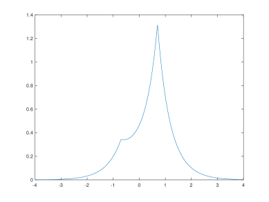
Figure 4.1. Plot of the spatial orbital $\phi\left(\mathbf{r}\right)$ for helium hydride $\mbox{HeH}^{+}$ on the line $\mathbf{r}=\left(0,0,x\right)$ connecting the two nuclear centers $\mathbf{R}_{1}=\left(0,0,-0.7\right)$ and $\mathbf{R}_{2}=\left(0,0,0.7\right)$.

4.2. Lithium Hydride, LiH

For our second example, we consider the Hartree-Fock equations for lithium hydride, LiH. The Hartree–Fock equations in this case are

(4.3) $$\mathcal{F}\phi_{j}\left(\mathbf{r}\right)=E_{j}\phi\left(\mathbf{r}\right),\ \ j=1,2,$$

where $\mathcal{F}=-\frac{1}{2}\Delta+\mathcal{V}_{ext}+2\mathcal{J}-\mathcal{K},$

$$\mathcal{J}\phi_{j}=\phi_{j}\left(-4\pi\Delta^{-1}\left(\left|\phi_{1}\right|^{2}+\left|\phi_{2}\right|^{2}\right)\right),$$

$$\mathcal{K}\phi_{j}=\phi_{1}\left(-4\pi\Delta^{-1}\left(\phi_{1}^{*}\phi_{j}\right)\right)+\phi_{2}\left(-4\pi\Delta^{-1}\left(\phi_{2}^{*}\phi_{j}\right)\right),$$

and

$$\mathcal{V}_{ext}\left(\mathbf{r}\right)=\frac{Z_{1}}{\left\|\mathbf{r}-\mathbf{R}_{1}\right\|}+\frac{Z_{2}}{\left\|\mathbf{r}-\mathbf{R}_{2}\right\|}.$$

For lithium hydride we have $Z_{1}=-3$, $Z_{2}=-1$ , $\mathbf{R}_{1}=\left(-3.15/2,0,0\right)$ and $\mathbf{R}_{2}=\left(3.15/2,0,0\right)$. We approximate potentials $Z_{1}/\left\|\mathbf{r}-\mathbf{R}_{1}\right\|$ and $Z_{2}/\left\|\mathbf{r}-\mathbf{R}_{2}\right\|$ and the Poisson kernel using (2.10) and the Green’s function $\mathcal{G}_{\mu}\left(r\right)$ in (2.11) using (2.12).

To solve (4.3), we initialize orbitals $\phi_{j}^{\left(0\right)}\left(\mathbf{r}\right),\ j=1,2$ as

$$\phi_{1}^{\left(0\right)}\left(\mathbf{r}\right)=e^{-\frac{\left\|\mathbf{r}-\mathbf{R}_{1}\right\|^{2}}{20}}\ \ \mbox{and}\ \ \phi_{2}^{\left(0\right)}\left(\mathbf{r}\right)=e^{-\frac{\left\|\mathbf{r}-\mathbf{R}_{2}\right\|^{2}}{20}}.$$

There are many possible initializations, e.g., we can use an approximation to $e^{-\left\|\mathbf{r}-\mathbf{R}_{1}\right\|}$ and $e^{-\left\|\mathbf{r}-\mathbf{R}_{2}\right\|}$ via Gaussian mixtures. Importantly, the initial approximation should be chosen so that the initial orbital energies are negative. After orthonormalizing the functions $\phi_{j}^{\left(0\right)}\left(\mathbf{r}\right)$, we compute the initial energies $E_{j}^{\left(0\right)}$ as the eigenvalues of the $2\times 2$ matrix defined in (2.5). We then set $\mu_{j}^{\left(0\right)},\ j=1,2$ using (2.6) and update the orbitals via (2.7).

Finally, when the desired accuracy is achieved, we compute the total energy $E_{tot}$ as

$$E_{tot}=\sum_{j=1}^{2}\left(E_{j}+\left\langle\left(-\frac{1}{2}\Delta+\mathcal{V}_{ext}\right)\phi_{j},\phi_{j}\right\rangle\right)+\frac{Z_{1}Z_{2}}{\left\|\boldsymbol{R}_{1}-\boldsymbol{R}_{2}\right\|}.$$

In this example, we choose an error tolerance of $\epsilon=10^{-6}$ for the reduction of terms in each group. We terminate the computation if $\left|E_{j}^{\left(m\right)}-E_{j}^{\left(m-1\right)}\right|<4\times 10^{-6}$ for $j=1,2$. After $28$ iterations, we arrived at the orbital energies $E_{1}=-2.451757267$ and $E_{2}=-0.297819313$ computed with absolute errors of $5.7\times 10^{-6}$ and $3.7\times 10^{-6}$, respectively, when compared with the reference energies $E_{1}=-2.451763$ and $E_{2}=-0.297823$ obtained using the MADNESS software. The computed total energy $E_{tot}=-7.9869324$ has an absolute error of $4.0\times 10^{-6}$ compared with the value $E_{tot}=-7.9869364$ evaluated in MADNESS. The total number of terms to represent orbitals $\phi_{1}\left(\mathbf{r}\right)$ and $\phi_{2}\left(\mathbf{r}\right)$ is $2185$ and $2569$. In Table 3, we show the number of terms in the global group $N_{global}$, the number of non-empty groups $N_{groups}$ and the maximum $N_{max}$, minimum $N_{min}$ and average $N_{ave}$ number of terms in the non-empty groups in the Gaussian mixture representations of $\phi_{1}$, $\phi_{2}$, $\mathcal{V}_{tot}\phi_{1}$ and $\mathcal{V}_{tot}\phi_{2}$ at the final step.

	$N_{global}$	$N_{group}$	$N_{max}$	$N_{min}$	$N_{ave}$
$\phi_{1}$	$218$	$26$	$108$	$1$	$75.7$
$\phi_{2}$	$217$	$31$	$107$	$1$	$75.9$
$\mathcal{V}_{tot}\phi_{1}$	$220$	$68$	$107$	$3$	$43.0$
$\mathcal{V}_{tot}\phi_{2}$	$215$	$69$	$107$	$4$	$46.2$

Table 3. The number of terms in the global group $N_{global}$ the number of non-empty groups $N_{group}$ and the maximum $N_{max}$, minimum $N_{min}$ and average $N_{ave}$ number of terms in these non-empty groups in $\phi_{1}$, $\phi_{2}$, $\mathcal{V}_{tot}\phi_{1}$ and $\mathcal{V}_{tot}\phi_{2}$ at the final step.

The resulting number of terms is again much smaller (about 100 times smaller) than that needed using MADNESS software and by a factor $\approx 2$ larger than that in [4], where the number of terms to represent the Slater-type orbitals is $1282$ and $1327$.

In Figure 4.2 we display the spatial orbitals $\phi_{1}\left(\mathbf{r}\right)$ and $\phi_{2}\left(\mathbf{r}\right)$ on the line $\mathbf{r}=\left(x,0,0\right)$ connecting the two nuclei locations $\mathbf{R}_{1}$ and $\mathbf{R}_{2}$.

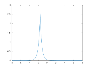
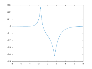
Figure 4.2. Plot of the spatial orbitals for lithium hydride, LiH, $\phi_{1}\left(\mathbf{r}\right)$ (left) and $\phi_{2}\left(\mathbf{r}\right)$ (right) on the line $\mathbf{r}=\left(x,0,0\right)$ connecting the two nucleus locations $\mathbf{R}_{1}=\left(-3.15/2,0,0\right)$ and $\mathbf{R}_{2}=\left(3.15/2,0,0\right)$.

Remark 5.

We implemented our code in Fortran90 and compiled it with the Intel Fortran Compiler version 19.0.1.144. All computations were performed on a single core (without any parallelization) of an Intel i7-6700 CPU at 3.4 GHz on a 64-bit Linux workstation with 64 GB of RAM. Currently it takes about $119$ seconds to solve the Hartree–Fock equations for $\mbox{HeH}^{+}$ and $999$ seconds to solve the equations for LiH. We made no attempt to optimize our implementation. While the reduction algorithm that splits Gaussian mixtures into groups (see Section 3) is trivially parallel, we did not take advantage of this property in the current version of our code. Since, for small molecules, the main cost is in reduction, we expect a speedup factor of about $20$, given the number of groups in Table 3. Such an acceleration factor should bring the timing close to that of MADNESS. We plan to do a careful speed comparison with existing methods separately.

Remark 6.

The reduction algorithm we used [12, Algorithm 1] is capable of achieving near full double precision accuracy if certain computations are carried out in quadruple precision. In addition to solving (4.1) and (4.3) using the reduction algorithm implemented in double precision and obtaining orbital energies $\approx 10^{-6}$, we continued iterations and switched to the reduction algorithm implemented in quadruple precision to improve the accuracy. We observed that, within several additional iterations, the orbital energies improved by gaining additional accurate digits. However, as pointed out in [12], the quadruple precision implementation is more than $10$ times slower than the double precision version (if the same accuracy is required). We do not include these results since, by modifying the reduction algorithm, it should be possible to avoid using quadruple precision. However, we note that, in most practical computations, an accuracy of $\approx 10^{-6}$ is typically sufficient.

5. Conclusions and further work

We presented a new adaptive algorithm for computing the electronic structure of molecules. Our approach is novel since we do not select a basis in advance and let the iteration for solving a system of integral equations identify the necessary functions to achieve a desired accuracy. The reduction algorithm developed in [12] selects the “best” subset of linearly independent terms after each operation that generates a large number of terms. These terms are Gaussians (identified by their parameters) and, since potentials and Green’s functions are also represented via Gaussian mixtures, all integrals are evaluated explicitly. Hence, in the algorithm, we only update the parameters of Gaussian mixtures.

We introduce in this paper a hierarchical subdivision of terms of Gaussian mixtures so that the computational cost of reduction is proportional to the number of nuclear centers. Although we did not implement a parallel version of our approach, it is clear that such an implementation will have a significant impact on the speed since reduction within each group of terms is independent of the other groups and computations are also mostly independent between orbitals.

We note that our method is less technical than that used in MADNESS (see [18]) and in [4] since our only tool is the reduction algorithm. We plan further work on our approach to verify its performance on large molecules.

References

- [1] B. Alpert. A class of bases in for the sparse representation of integral operators. SIAM J. Math. Anal, 24(1):246–262, 1993.
- [2] G. M. J. Barca and P-F. Loos. Three- and four-electron integrals involving gaussian geminals: fundamental integrals, upper bounds, and recurrence relations. The Journal of chemical physics, 147(2):024103, 2017.
- [3] G. Beylkin, R. Coifman, and V. Rokhlin. Fast wavelet transforms and numerical algorithms, I. Comm. Pure Appl. Math., 44(2):141–183, 1991. Yale Univ. Technical Report YALEU/DCS/RR-696, August 1989.
- [4] G. Beylkin and T. S. Haut. Nonlinear approximations for electronic structure calculations. Proc. R. Soc. A, 469(20130231), 2013.
- [5] G. Beylkin and M. J. Mohlenkamp. Numerical operator calculus in higher dimensions. Proc. Natl. Acad. Sci. USA, 99(16):10246–10251, August 2002.
- [6] G. Beylkin and M. J. Mohlenkamp. Algorithms for numerical analysis in high dimensions. SIAM J. Sci. Comput., 26(6):2133–2159, July 2005.
- [7] G. Beylkin, M. J. Mohlenkamp, and F. Pérez. Preliminary results on approximating a wavefunction as an unconstrained sum of Slater determinants. Proceedings in Applied Mathematics and Mechanics, 7(1):1010301–1010302, 2007.
- [8] G. Beylkin, M. J. Mohlenkamp, and F. Pérez. Approximating a wavefunction as an unconstrained sum of Slater determinants. Journal of Mathematical Physics, 49(3):032107, 2008.
- [9] G. Beylkin and L. Monzón. On approximation of functions by exponential sums. Appl. Comput. Harmon. Anal., 19(1):17–48, 2005.
- [10] G. Beylkin and L. Monzón. Approximation of functions by exponential sums revisited. Appl. Comput. Harmon. Anal., 28(2):131–149, 2010.
- [11] G. Beylkin, L. Monzón, and I. Satkauskas. On computing distributions of products of random variables via Gaussian multiresolution analysis. Appl. Comput. Harmon. Anal., 2017. see also arXiv:1611.08580.
- [12] G. Beylkin, L. Monzon, and X. Yang. Reduction of multivariate mixtures and its applications. J. Comp. Phys., 383:94–124, 2019. see also https://arxiv.org/abs/1806.03226.
- [13] S. F. Boys. The integral formulae for the variational solution of the molecular many-electron wave equations in terms of gaussian functions with direct electronic correlation. Proceedings of the Royal Society of London Series A- Mathematical and Physical Sciences, 258(1294):402, 1960.
- [14] I. Daubechies. Ten Lectures on Wavelets. CBMS-NSF Series in Applied Mathematics. SIAM, 1992.
- [15] G. Fann, R. Harrison, G. Beylkin, R. Hartman-Baker, J. Jia, W. A. Shelton, and S. Sugiki. MADNESS applied to density functional theory in chemistry and physics. J. of Physics, Conference Series, 78:012018, 2007. doi:10.1088/1742-6596/78/1/012018.
- [16] L. Genovese, A. Neelov, S. Goedecker, T. Deutsch, S.A. Ghasemi, A. Willand, D. Caliste, O. Zilberberg, M. Rayson, and A. Bergman. Daubechies wavelets as a basis set for density functional pseudopotential calculations. The Journal of chemical physics, 129(1):014109, 2008.
- [17] E. Giner, B. Pradines, A. Ferté, R. Assaraf, A. Savin, and J. Toulouse. Curing basis-set convergence of wave-function theory using density-functional theory: a systematically improvable approach. The Journal of chemical physics, 149(19):194301, 2018.
- [18] R. J. Harrison, G. Beylkin, F. A. Bischoff, J. A. Calvin, G. I. Fann, J. Fosso-Tande, D. Galindo, J.R Hammond, R. Hartman-Baker, J.C. Hill, J. Jia, J.S. S. Kottmann, M-J. Y. Ou, L.E. Ratcliff, M.G. Reuter, A.C. Richie-Halford, N.A. Romero, H. Sekino, W.A. Shelton, B.E. Sundahl, W.S. Thornton, E.F. Valeev, A. Vázquez-Mayagoitia, N. Vence, and Y. Yokoi. MADNESS: a multiresolution, adaptive numerical environment for scientific simulation. SIAM J. Sci. Comput., 38(5):S123–S142, 2016. see also arXiv preprint arXiv:1507.01888.
- [19] R.J. Harrison, G.I. Fann, T. Yanai, Z. Gan, and G. Beylkin. Multiresolution quantum chemistry: basic theory and initial applications. J. Chem. Phys., 121(23):11587–11598, 2004.
- [20] S. R. Jensen, S. Saha, J. A. Flores-Livas, W. Huhn, V. Blum, S. Goedecker, and Luca Frediani. The elephant in the room of density functional theory calculations. The Journal of Physical Chemistry Letters, 8(7):1449–1457, 2017.
- [21] M. H. Kalos. Monte Carlo calculations of the ground state of three- and four-body nuclei. Phys. Rev. (2), 128:1791–1795, 1962.
- [22] M. H. Kalos. Monte Carlo integration of the Schrödinger equation. Trans. New York Acad. Sci. (2), 26:497–504, 1963/1964.
- [23] A. Komornicki and H. F. King. A general formulation for the efficient evaluation of n-electron integrals over products of gaussian charge distributions with gaussian geminal functions. The Journal of chemical physics, 134(24):244115, 2011.
- [24] J.V.L. Longstaff and K. Singer. The use of gaussian (exponential quadratic) wave functions in molecular problems. ii. wave functions for the ground state of the hydrogen atom and of hydrogen molecule. Proc. R. Soc. London Ser. A-Math., 258(1294):421, 1960.
- [25] F. A. Pahl and N. C. Handy. Plane waves and radial polynomials: a new mixed basis. Molecular Physics, 100:3199–3224, 2002.
- [26] R. G. Parr and W. Yang. Density-Functional Theory of Atoms and Molecules. Number 16 in The International Series of monographs on Chemistry. Oxford Univ. Press, New york, 1989.
- [27] T. Shiozaki and S. Hirata. Grid-based numerical hartree-fock solutions of polyatomic molecules. Phys. Rev. A, 76:040503, Oct 2007.
- [28] B. Simon. Quantum mechanics for Hamiltonians defined as quadratic forms. Princeton University Press, 1971.
- [29] K. Singer. The use of gaussian (exponential quadratic) wave functions in molecular problems. i. General formulae for the evaluation of integrals. Proc. R. Soc. London Ser. A-Math., 258(1294):412, 1960.
- [30] A. Szabo and N. S. Ostlund. Modern Quantum Chemistry: Intro to Advanced Electronic Structure Theory. Dover publications, 1996.
- [31] T. Yanai, G.I. Fann, Z. Gan, R.J. Harrison, and G. Beylkin. Multiresolution quantum chemistry: Analytic derivatives for Hartree-Fock and density functional theory. J. Chem. Phys., 121(7):2866–2876, 2004.
- [32] T. Yanai, G.I. Fann, Z. Gan, R.J. Harrison, and G. Beylkin. Multiresolution quantum chemistry: Hartree-Fock exchange. J. Chem. Phys., 121(14):6680–6688, 2004.