On Radiation Reaction in Classical Electrodynamics

Abstract

The Lorentz-Abraham-Dirac equations (LAD) may be the most commonly accepted equation describing the motion of a classical charged particle in its electromagnetic field. However, it is well known that they bear several problems. In particular, almost all solutions are dynamically unstable, and therefore, highly questionable. As shown by Spohn et al., stable solutions to LAD can be approximated by means of singular perturbation theory in a certain regime and lead to the Landau-Lifshitz equation (LL). However, for two charges there are also counter-examples, in which all solutions to LAD are unstable. The question remains whether better equations of motion than LAD can be found to describe the dynamics of charges in the electromagnetic fields. In this paper we present an approach to derive such equations of motions, taking as input the Maxwell equations and a particular charge model only, similar to the model suggested by Dirac in his original derivation of LAD in 1938. We present a candidate for new equations of motion for the case of a single charge. Our approach is motivated by the observation that Dirac’s derivation relies on an unjustified application of Stokes’ theorem and an equally unjustified Taylor expansion of terms in his evolution equations. For this purpose, Dirac’s calculation is repeated using an extended charge model that does allow for the application of Stokes’ theorem and enables us to find an explicit equation of motion by adapting Parrott’s derivation, thus avoiding a Taylor expansion. The result are second order differential delay equations, which describe the radiation reaction force for the charge model at hand. Their informal Taylor expansion in the radius of the charge model used in the paper reveals again the famous triple dot term of LAD but provokes the mentioned dynamical instability by a mechanism we discuss and, as the derived equations of motion are explicit, is unnecessary.

I The Lorentz-Abraham-Dirac equation

Finding an equation of motion for a classical charged particle in its classical radiation field is a very old problem; see the exhaustive references in Rohrlich (2007); Lyle (2010); Spohn (2004); Penrose and Mermin (1990). Since point particles lead to divergences within classical electrodynamics, different remedies have been explored. One approach is to modify Maxwell’s equations as has been done by Born-Infeld Born and Infeld (1934) or Bopp-Podolsky Podolsky and Schwed (1948), see also Kiessling (2004, 2019) and other approaches such as Feynman (1948) and more recently Raju and Raju (2011). Another approach is to introduce an extended charge model as it has been done by Abraham M. (1906), Lorentz Lorentz (2007), and many others Caldirola (1956). Beside their tension with regard to Lorentz invariance, very early it was realized that such models introduce an electrodynamic inertial mass for which Dirac proposed his famous mass renormalization program to investigate the corresponding point charge limit Dirac (1938); see Gralla et al. (2009) for a recent approach in controlling such a point-charge limit. An entirely different approach was taken by Wheeler and Feynman Wheeler and Feynman (1945) who were able to derive an radiation reaction equation from an action-at-a-distance principle at the cost of introducing advanced and retarded delays in the equations of motion. Beside the problem of self-interaction, it is interesting to note that in the case of more than one interacting point-charges there are further difficulties connected to the emergence of singular fronts in the solutions to the Maxwell equations Deckert and Hartenstein (2016).

Although all these approaches are quite different, the Lorentz-Abraham-Dirac (LAD) equations of motion almost always appear as a limiting case. Hence, whatever the fundamental equations of motion for a classical charged particle in its radiation field are, the general consensus would likely be that a connection to the LAD equations should be possible in a certain limit. At this point it is interesting to note, as pointed out in Spohn (2004), that there is no experiment that could measure the radiative corrections to the corresponding charge trajectories introduced by any of the candidates of radiation reaction equations with sufficient precision even though, in a large regime, the phenomenon of radiation reaction is a purely classical effect. However, recently radiation reaction has attracted new attention Cole et al. (2018); Sheffer et al. (2018); Wistisen et al. (2018), which gives hope that accurate experimental data will be provided in the future. The LAD equations are given by

$$ma^{\alpha}=qF^{\alpha\beta}(z)\,u_{\beta}+\frac{2q^{2}}{3}\left(\frac{da}{d\tau}^{\alpha}+a^{\beta}a_{\beta}u^{\alpha}\right)\,,$$ (1)

where $z^{\alpha}(\tau)$, $u^{\alpha}(\tau)$, and $a^{\alpha}(\tau)$ denote the relativistic position, velocity, and acceleration four-vectors of the charge under examination, respectively, with $\tau$ being the world-line parameter, e.g., the proper time. Moreover, $m$ denotes its effective inertial mass, $q$ its charge, and $F^{\alpha\beta}$ is the field strength tensor of the electromagnetic fields of all other particles that may also include an additional external field. Throughout the paper we set the speed of light to $c=1$. Hence, the first expression on the right-hand side of (1) is the Lorentz force due to all other charges and the external field. The second expression on the right-hand side describes the so-called self-interaction, i.e., the interaction of the charge under consideration with its own radiation field. Since this term involves a third derivative of the world-line $z^{\alpha}(\tau)$ one also refers to it as radiation friction term. There is no straight forward way to arrive at expression (1). In Dirac’s paper Dirac (1938) it is the zero order term of the total self-force, i.e., the Lorentz force on the charge through its own Maxwell field, expanded in a Taylor series about the radius $\epsilon$ of the charge distribution. In Dirac computation, there is also a term of order $\epsilon^{-1}$. This term is proportional to the acceleration. It is usually brought to the left side of equation (1) and absorbed in the mass coefficient such that

$$\color[rgb]{.7,.2,.2}\color[rgb]{0,0,0}m_{\text{ren}}=m+\frac{q^{2}}{2\epsilon}\,,$$ (2)

where $m$ is the bare inertial mass of the charged particle and $m_{\text{ren}}$ the renormalized one. The usual argument in the text books is that the bare inertial mass and the inertial mass originating from the field energy, cannot be separated by any experiment and only their sum can be observed. While this is surely a sensible argument, it has to be emphasized that for $\epsilon$ smaller than the classical electron radius $e^{2}/(4\pi\epsilon_{0}m_{e}c^{2})$ the argument implies that the bare mass $m$ has to be negative in order to ensure that the electron attains the inertial mass known from experiments. It has been emphasized that this implication even holds true for any extended charge model and is not just an artifact of the limit $\epsilon\to 0$.

Although this renormalization procedure has been the reason for some concern it seems to be unavoidable if one is not willing to modify Maxwell equations or the Lorentz force and still wants to describe a relativistic particle as light and small as the electron seems to be. It is also important to note that there is no easy way out, e.g., by claiming that on such scales quantum electrodynamics (QED) would have to be invoked to describe the phenomenon of radiation reaction. First, QED has been plagued by exactly the same problem of infinities through self-interaction – there, called the ultraviolet divergence of the photon field, which has prevented the formulation of a mathematically well-defined Schrödinger-type equation for the dynamics ever since. And second, in a large regime the quantum corrections do not seem to play an important role. For ultra-strong electromagnetic backgrounds, however, observable signatures of the nonlinear quantum vacuum as well as a subtle interesting interplay with radiation reaction are to be expected King et al. (2014). Due to recent progress in technology (CALA, ELI) the correct formulation of both the classical and quantum dynamics of radiation reaction has regained high priority.

All higher order terms in $\epsilon$ in Dirac’s computation depend on assumptions about the geometry of the current distribution and usually are neglected by taking the limit $\epsilon\to 0$. By all means, it is justified to worry if taking the limit $\epsilon\rightarrow 0$ leads to a well-behaved equation of motion. Foremost, this limit is taken at a fixed instant in time only. However, to control the difference of potential solutions for varying $\epsilon$, bounds at least uniform on a time interval are required. Dirac himself pointed out that even for the case of a single particle in the absence of external fields there is but one physical sensible LAD solution, namely the straight line, while all other solutions describe charges that accelerate increasingly in time.

An example of how neglecting higher order terms in a Taylor series can lead to unstable solutions is given in chapter I.3 of this paper. One example for such a solution of (1) is

$$u^{\alpha}(\tau)=\begin{pmatrix}\cosh\left(e^{\frac{3m}{2q^{2}}\tau}\right)\\ 0\\ 0\\ \sinh\left(e^{\frac{3m}{2q^{2}}\tau}\right)\end{pmatrix}\,,$$ (3)

which are obviously highly questionable. They are referred to as run-away solutions. Believing in the physical relevance of the LAD equations implies finding a way to rule out run-away solutions. Since the LAD equations are third order equations, the initial value problem admits points from a nine-dimensional manifold, i.e., position, momentum, and acceleration three-vectors at one time instant. One approach is using singular perturbation theory in the leading part of the second term of (1) in the approximation of slowly varying external fields, which results in the Landau-Lifschitz (LL) equation; see Spohn (2004) for an extensive overview. In the perturbative regime and for the case of a single charge it can be shown that all stable solutions have initial values on a six-dimensional sub-manifold, i.e., comprising position and momentum three-vectors at an instant of time only from which the “correct” initial acceleration can in principle be computed. The stable solutions are the ones that are approximates by the LL equations; see Di Piazza (2008) for an exact solution. The LL equations are therefore dynamically well behaved and also useful for practical calculations in there range of validity. Strictly speaking, however, they are in character more an approximation rather than a fundamental equations. The strategy to simply select the “correct” initial acceleration fails in more complicated systems. This is shown by Eliezer Eliezer (1943) by giving a counter example. Eliezer considers two oppositely charged particles moving towards each other in a symmetric fashion and proves that for all initial accelerations, the particles turn around at some point before they collide and fly apart with ever increasing acceleration. His result implies that there exist cases in which the LAD equations do not seem to give a satisfactory answer. The example by Eliezer is elaborately discussed by Parrott in Parrott (2012). At the very least for those cases, new equations of motion are needed, but also in general, having access only to stable approximate solutions does not seem to be entirely satisfactory.

This present unsatisfactory situation is the main motivation for our work. We will reconsider Dirac’s and Parrot’s derivations of radiation reaction equations and by adapting and extending them propose new exact equations of motion, i.e., without making use of a Taylor expansion.

I.1 Dirac’s original derivation

To obtain “better” equations of motion, as compared to LAD, it is important to understand the shortcomings in their derivation. Dirac makes use of a point particle as the model of a charged particle. His approach has the advantage that he does not need to be concerned about the inner structure of the particle. The disadvantage, however, is that the Lorentz force cannot be used right away because the fields are singular in the vicinity of the point charge. Instead of using the Lorentz force to infer the equation of motion, Dirac uses the concept of energy-momentum conservation as a starting point since the change in momentum of the charge can be expressed by means of energy-momentum tensor

$$4\pi T^{\alpha\beta}=F^{\alpha\gamma}F_{\gamma}^{\beta}+\frac{1}{4}\eta^{\alpha\beta}F^{\gamma\delta}F_{\gamma\delta}\,.$$ (4)

In (4) the quantity $\eta^{\alpha\beta}$ is the metric tensor having the signature $\eta=\operatorname{diag}(1,-1,-1,-1)$. Now let $V(\tau_{1},\tau_{2})$ be a smooth space-time region, which encompasses an interval of the world-line of the charge given by $z^{\alpha}$ with the entry and exit space-time points $z^{\alpha}(\tau_{1})$ and $z^{\alpha}(\tau_{2})$, respectively. Dirac implicitly argues in the spirit of Stokes’ theorem that the volume integral over $V(\tau_{1},\tau_{2})$ of the divergence of $T^{\alpha\beta}$ equals the surface integral over the boundary $\partial V(\tau_{1},\tau_{2})$ of the energy-momentum flow out of the volume. Thus, we obtain

$$P^{\alpha}(\tau_{2})-P^{\alpha}(\tau_{1})=\int_{\tau_{1}}^{\tau_{2}}d\tau\,F^{\alpha}(z(\tau))$$

$$=\int_{\tau_{1}}^{\tau_{2}}d\tau\,qF^{\alpha\beta}(x)u_{\beta}(\tau)$$

$$=\int_{V(\tau_{1},\tau_{2})}d^{4}x\int d\tau\,qF^{\alpha\beta}(x)\,u_{\beta}(\tau)\,\delta^{4}(z^{\beta}(\tau)-x^{\beta})$$

$$=\int_{V(\tau_{1},\tau_{2})}d^{4}x\,F^{\alpha\beta}(x)\,j_{\beta}(x)$$

$$=-\int_{V(\tau_{1},\tau_{2})}d^{4}x\,\partial_{\beta}T^{\alpha\beta}(x)$$

$$=-\int_{\partial V(\tau_{1},\tau_{2})}d^{3}x_{\beta}\,T^{\alpha\beta}(x)\,,$$ (5)

where the difference $P^{\alpha}(\tau_{2})-P^{\alpha}(\tau_{1})$ in (I.1) is the total change of momentum of the point charge along the world-line $z^{\alpha}(\tau)$. The surface measure times the normal four-vector $n^{\beta}(x)$ on the boundary $\partial V(\tau_{1},\tau_{2})$ is denoted by $d^{3}x^{\beta}$. In (I.1) use has been made of the definition of the current density of a point particle

$$j^{\alpha}\left(x\right)=q\int d\tau\,u^{\alpha}(\tau)\,\delta^{4}\left(z^{\beta}(\tau)-x^{\beta}\right)\,.$$ (6)

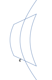
Figure 6: Dirac’s tube, it is defined by moving the length $\epsilon$ along the hyperplane of simultaneity in the rest frame in all directions between $\tau_{1}$ and $\tau_{2}$.

Unfortunately, Stokes’ theorem is not applicable in the context of the assumptions made by Dirac as the fields $F^{\alpha\beta}$ that enter $T^{\alpha\beta}$ are not smooth but singular on $V(\tau_{1},\tau_{2})$ due to the point charge model. As a matter of fact, neither the left- nor right-hand side of equation (I.1) is well-defined. In the expressions on the right-hand side, however, the field divergences appear only at the points where the particle enters and leaves the integration volume $V(\tau_{1},\tau_{2})$. In order to treat the integrations there Dirac introduced a cut-off to remove the divergent contributions. The definition and physical meaning of a cut-off is discussed in chapter I.2. Dirac argues that the shape of the integration volume does not influence the final result since the divergence of the energy-momentum tensor vanishes at points with no charge present. Hence, only the amount of the charge inside the volume matters and not its shape. However, we will see that this is not true for the point-charge model assumed by Dirac and that the shape of the volume actually matters at the points where the world-line penetrates the surface of the volume. Next, Dirac picks as the volume $V(\tau_{1},\tau_{2})$ a four dimensional tube consisting of the union of spheres with radii of the size of the cut-off parameter $\epsilon$ in each rest frame between the two fixed entry and exit space-time points at $z^{\alpha}(\tau_{1})$ and $z^{\alpha}(\tau_{2})$. Dirac’s tube is visualized in Fig. 6. Dirac divides the surface integration into two parts, an integration over the lateral surface of his tube and an integration over the caps. While Dirac presents an explicit calculation of the contribution of the lateral surface to the energy-momentum tensor, he is not performing the cap integrations, which would diverge for the point particle. Instead, he guesses that the cap integrals are equivalent to the kinetic term $ma^{\alpha}$. Dirac’s guess in fact implies a cut-off in the fields since the contribution of the cap integrals to the energy-momentum tensor is assumed to be zero. The remaining integral over the lateral surface of the tube is always close to the world-line. For the evaluation of the fields at the lateral surface of the tube Dirac needs the retarded proper time. An explicit expression of the latter, however, is generally not available. Hence, Dirac introduces a Taylor series in the cut-off parameter $\epsilon$ and assumes that all higher order terms of the latter only give negligible contributions to the dynamics provided the cut-off parameter is small enough. Dirac’s assumption, however, is unjustified as we will discuss later by means of a counter example. By differentiation of (I.1) with respect to $\tau_{2}$ Dirac obtains an expression for the Lorentz force at time $\tau_{2}$. To calculate the surface integrals implied in (I.1), Dirac determines the corresponding Liénard-Wiechert potentials and calculates the field-strength tensor. Finally, he computes the energy-momentum tensor and carries out the integrations as discussed. After all these steps and absorbing terms of the order $\epsilon^{-1}$ into the bare inertial mass according to (2), he arrives at (1).

These issues and how to circumvent them will be the content of the next sections. The outline of the paper is as follows. In chapter I.2 it is discussed that the assumption of a cut-off and the requirement of consistency with the Maxwell equations imply an extended charge model. In chapter I.3 it is shown that the Taylor series mentioned before cannot be used. In chapter I.4 the approach pursued by Parrott is discussed, which allows to avoid the Taylor series. In the same chapter a constraint that seems to be missing in Parrott’s calculation on the tube geometry is also discussed, which arises from the fact that the total self-force on the particle is given by integration over the Lorentz force density acting on the extended particle. This leads to the conclusion that the caps of the tube have to be hyperplanes of simultaneity in the co-moving reference frame of the charge. In chapter II an expression for the radiation reaction force is derived, which is the first main result of this paper. In chapter III new equations of motion and a discussion of the resulting radiation reaction force are given which represents the second main result of this work.

I.2 Interpretation of the cut-off

There is no obvious reason why the cap integrals of the energy-momentum tensor appearing in (I.1) at $\tau_{1}$ and $\tau_{2}$ with radius $\epsilon$ can be neglected. No matter how small $\epsilon$ is the corresponding integrals give infinite contributions, which in view of Stokes’ theorem also depend on the geometry of the corresponding cut-off (for $\epsilon\to 0$ also on the mode of convergence) and therefore cannot be ignored. In Dirac’s derivation the cap contributions are dropped, nevertheless. However, it is possible to give a reasonable interpretation of Dirac’s cut-off even without taking the limit. We note that the cap integrations at $\tau_{1}$ and $\tau_{2}$ correspond to integrations over spheres at $\tau_{1}$ and $\tau_{2}$. Obviously, the integrals over a sphere with radius $\epsilon$ can be ignored if and only if the value of the sum of the integrands for the spheres at $\tau_{1}$ and $\tau_{2}$ is zero. This is not the case for a point particle but it is certainly the case for a specific class of charge current distributions. The simplest example of such a distribution is one which has no fields inside of such a sphere. Thus, dropping the cap integrals in (I.1) implies that the original field strength tensor of a point charge is replaced by a field strength tensor which is zero inside a cut-off region and identical to the field strength tensor of the point particle outside of it. The corresponding distribution can be calculated with the help of Maxwell’s equations

$$\partial_{\alpha}F^{\alpha\beta}_{\epsilon}=4\pi j_{\epsilon}^{\beta}\,,$$ (7)

where $j^{\beta}_{\epsilon}$ is the new distribution due to the cut-off $\epsilon$. Stokes’ theorem shows that this distribution is located on the surface of the sphere. But it is not necessarily homogeneous and, hence, does not imply that the introduction of such a cut-off is nothing else than replacing the original point charge by an extended current distribution on a sphere and that taking the limit $\epsilon\to 0$ means shrinking the radius of the distribution down to zero. In contrast, the general situation is more subtle as even the limit $\epsilon\to 0$ involves a choice, i.e., the mode of convergence of the particularly chosen current model to the point-charge limit.

Throughout this work we will, however, keep $\epsilon>0$. Since the field strength tensor of such a current distribution is free of divergences, Stokes’ theorem can be applied in the argument in (I.1).

I.3 Taylor expanding in the cut-off

From the discussion in chapter I.2 we conclude that an extended current distribution has to be considered. We assume that the current distribution is spherical with the cut-off radius $\epsilon>0$. This choice implies that the radiation reaction force will then involve a delay due to the finite speed of light of the field propagating through the extended particle. This delay is a shared feature of all extended charge models as can be seen in Sommerfeld (1904), Caldirola (1956) or Levine et al. (1977).

It is shown in this paper that the radiation reaction force indeed leads to 2nd order delay-differential equations and that the third order derivative $da^{\alpha}/d\tau$ in (1) originates from a Taylor expansion in $\epsilon$ of the delayed radiation reaction force. As it is well-known Driver (1977); Raju and Raju (2011); Walther (2014), dropping all higher order terms in $\epsilon$ to obtain (1) can lead to a severe change in the corresponding space of solutions as can be demonstrated by the following simple example:

$$z(t)=z(t-\epsilon).$$ (8)

The solutions to (8) are obviously periodic functions with period length $\epsilon$. Taylor expanding informally the right-hand side of (8) up to 2nd order and truncating the rest gives

$$z(t)=z(t)-\epsilon\dot{z}(t)+\frac{\epsilon^{2}}{2}\ddot{z}(t)\,.$$ (9)

One solution of this equation is

$$z(t)=e^{\frac{2t}{\epsilon}}\,.$$ (10)

This is clearly no solution to the original equation (8). It exhibits a behavior much like the unstable solutions of the LAD equation, the so-called run-away solutions. The reason why a Taylor expansion of (8) in $\epsilon$ fails can be explained as follows. Although the right hand sides of the two equations (8) and (9) for comparable initial conditions and at a fixed instant in time differ only by a term of the order of $\epsilon^{3}$ the implication is not that also the two respective solutions remain close to each other for other times. For the latter one needs a uniform estimate of the difference of the respective right-hand sides of (8) and (9) on at least a time interval, e.g., in the spirit of Grönwall’s lemma.

For our simple example we can readily compute the contribution coming from the neglected higher-order terms. They are

$$\sum_{n=3}^{\infty}\frac{(-\epsilon)^{n}}{n!}z^{(n)}(t)=\left(e^{-2}-1\right)\,z(t)\,.$$ (11)

Thus, the smallness of higher-order terms does not directly depend on $\epsilon$ but on the norm of the corresponding solution $z(t)$. The latter will in general depend on $\epsilon$ but in a much more subtle way. Controlling it in $\epsilon$ therefore requires a careful mathematical analysis. It is not sufficient to simply control the right-hand side of (8) at one instant in time. The emergence of the run-away solutions as (10) after a Taylor expansion neglecting higher orders in our simple example shows that higher order terms in $\epsilon$ cannot be ignored in general.

The conclusion is that we have to repeat Dirac’s calculation taking the terms to all orders into account. This appears not to be feasible for the tube Dirac has chosen. However, the calculation can be carried out as outlined by Parrott Parrott (2012) for a tube suggested by Bhabha. In chapter I.4 the result of Parrott’s calculation and the need for modifications of the tube at the caps used in our paper are discussed.

I.4 Meaningful caps

In his book Parrott Parrott (2012) repeats Dirac’s calculation without the Taylor expansion that Dirac uses. We argue shortly why Parrott’s calculation still has to be modified in order to lead to a meaningful candidate for an equation of motion with radiation damping.

Parrott evaluates the time integral over the force in (I.1), which equals the time integral over the Lamor formula

$$\int^{\tau_{2}}_{\tau_{1}}d\tau\,F^{\alpha}(z(\tau))$$

$$=\int^{\tau_{2}}_{\tau_{1}}d\tau\,(2q^{2}/3)\,(a^{\beta}a_{\beta}\,u^{\alpha})(\tau)\,.$$ (12)

Parrott does not carry out the time derivative of the expression $\int^{\tau_{2}}_{\tau_{1}}d\tau\,F^{\alpha}(z(\tau))$ in (I.4), which cannot be computed for the tube used by Parrott. A valid force, as we argue, is however only obtained by performing the time derivative of $\int^{\tau_{2}}_{\tau_{1}}d\tau\,F^{\alpha}(z(\tau))$. As a consequence, Parrott’s result may not be interpreted easily as a force, which also manifests itself in the fact that the Lamor term is in general not orthogonal to the four-velocity. Instead, Parrott argues that the times $\tau_{1}$ and $\tau_{2}$ are somehow special. He requires that the accelerations at $\tau_{1}$ and $\tau_{2}$ are zero. According to him, this is a necessary condition if the result of the calculation must not depend on the form of the caps. As a consequence, the time derivative in Parrott’s case is only possible for time regions with zero acceleration, but for zero acceleration there is no radiation reaction force. Since for $a^{\alpha}(\tau_{1})=0$ and $a^{\alpha}(\tau_{2})=0$ one finds that

$$\int^{\tau_{2}}_{\tau_{1}}d\tau\frac{2q^{2}}{3}\frac{d}{d\tau}a^{\alpha}(\tau)=0$$ (13)

holds, Dirac’s and Parrott’s results agree when integrating Dirac’s force over time with the acceleration conditions above. Also Dirac’s result for the radiation reaction force depends on the choice of the caps since Stokes’ theorem cannot be applied the way Dirac argues as we have outlined in chapter I.1.

The problem with Stokes’ theorem can be illustrated nicely with the help of an analogy. Let us consider the example of a point charge resting at the origin of the coordinate system for which the fields are only the Coulomb fields.

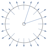
Figure 1: The left plot shows the flow of the Coulomb field of a resting point charge through a sphere respectively a spherical sector. The right plot shows the same situation for a charge corresponding to Coulomb fields with a cut-off at radius $\epsilon$, which implies a charge model of a hollow sphere of radius $\epsilon$ in the rest frame.

An integration of the flow of the electric field over the entire sphere around the origin gives $4\pi\,q$, where $q$ is the charge at the origin. On the other hand, an integration over a sector of the sphere gives $\Omega\,q$, where $\Omega$ is the solid angle of the spherical sector. The lateral walls of the spherical sector do not contribute since their normal vector is orthogonal to the electric field. According to Stokes’ theorem, as used in Dirac’s derivation, it is expected that volumes containing the same amount of charge yield the same surface integrals of the flow of the fields. Apparently, for a point charge on the surface the application of Stokes’ theorem does not yield unique results in contrast to what is expected. To proceed with the analogy we cut off the field the way Dirac does and as we have outlined in chapter I.2. According to (7) this implies that the point charge in its rest frame is replaced by a homogeneously charged hollow sphere with radius $\epsilon$. On its outside the hollow charge distribution generates the same fields as a point charge while there are no fields inside of it. For the hollow charge the integral over the entire sphere yields the total charge $4\pi\,q$ and the integral over a spherical sector the fraction $\Omega\,q$ as before. In contrast to the situation of a point charge the integration volumes now contain different amounts of charge in agreement with Stokes’ theorem as illustrated in Fig. 1. Apparently, the theorem of Stokes’ can be applied after the introduction of the cut-off. The implication is that the amount of charge contained in the tubes depends on the choice of the caps as is illustrated with the help of Fig. 2.

Now we try to determine which amount of charge the tube should contain.

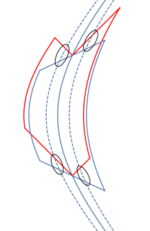
Figure 2: Due to the cut-off, the charge is distributed around the world-line given by the blue solid line. The distributed charge is represented by the dashed lines. Even though the red and the blue tubes start and end at the same points of the world-line they contain different amounts of charge as is highlighted by the circles. Note that the time axis is vertical and the space axis horizontal. Also note that for any given definition of the caps due to the theorem of Stokes the tube radius is irrelevant as long as it is at least equal or larger than $\epsilon$. In the paper we set the latter equal to $\epsilon$ contrary to the sketch in the figure since then the cap contributions are identical to zero.

Since we are dealing with an extended current distribution, (I.1) describes an integral over a force density which should be equal to the momentum difference $P^{\alpha}(\tau_{2})-P^{\alpha}(\tau_{1})$, where $P^{\alpha}(\tau)$ is the total momentum of the extended particle. Performing the derivative of the force integral in (I.1) with respect to $\tau_{2}$ leads to

$$\frac{dP^{\alpha}(\tau)}{d\tau}=F^{\alpha}(\tau)\,.$$ (14)

To obtain the correct total force $F^{\alpha}$ and total momentum $P^{\alpha}$ in (14) from the force and momentum densities in (I.1) the correct integration regions have to be used. To obtain them and hence the correct tube geometry, we consider the non-relativistic limit

$$\vec{P}(t)=\int_{V}d^{3}r\,\vec{p}\left(t,\vec{r}\right)\,,$$ (15)

where $\vec{p}\left(t,\vec{r}\right)$ is the momentum density. The naive relativistic generalization

$$P^{\alpha}(\tau)=\int dx_{1}\wedge dx_{2}\wedge dx_{3}\,p^{\alpha}(x^{\beta})$$ (16)

is not a Lorentz vector since the integration region, given by the three form $dx_{1}\wedge dx_{2}\wedge dx_{3}$, is not a Lorentz scalar. The reason for this is, that equal time surfaces get tilted under Lorentz transformations. To find a relativistic generalization an expression for the integration region is needed which is a Lorentz scalar and reduces to (16) in the co-moving coordinate frame in the non-relativistic limit. We consider the normal vector of the integration region in equation (16). Formally it can be obtained with the help of the Hodge dual and has the simple form $(1,0,0,0)$ corresponding to $dt$. Since $u^{\alpha}dx_{\alpha}$ is a Lorentz scalar, which reduces to $dt$ in the co-moving coordinate frame, a good candidate for the integration region is given by the Hodge dual of $-u^{\alpha}dx_{\alpha}$. This implies, that the integration in (I.1) should be performed over hyperplanes of simultaneity in the rest frame.

The time derivative in equation (14) can be interpreted as the limit $\tau_{1}\rightarrow\tau_{2}$. Since in this limit the tube is only allowed to contain charge located on a hyperplane of simultaneity in the rest frame at time $\tau_{2}$, the caps also have to be hyperplanes of simultaneity in their own rest frames, as can be seen in Fig. 3. By this line of reasoning we conclude that Dirac’s choice of the caps is the right one and Parrott’s extra condition $a^{\alpha}(\tau_{i})=0$ is not needed for Dirac’s and our caps.

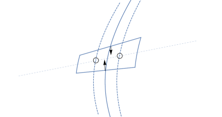
Figure 3: The current distribution is represented by the vertical dashed lines. After taking the limit represented by the arrows only charge on the hyperplane of simultaneity in the co-moving frame of reference represented by the horizontal dashed line must be contained inside the tube. This charge is marked by the two circles for better visibility. Hence, the caps are hyperplanes of simultaneity in the co-moving reference frame as can be seen from the plot.

In chapter II we explain how to construct a tube in such a way that both Parrott’s approach as well as Dirac’s caps can be used to give a consistent derivation of a meaningful force. It is worth mentioning that the results in the next chapters hold for any finite value of $\epsilon$ and that the limit $\epsilon\rightarrow 0$ is never required for explicit calculations.

II The radiation reaction force

In this chapter we present the first main result of the paper, which in part is based on Dirac’s and Parrot’s work but also goes beyond it by avoiding the issues discussed in Section I.1. We provide new force candidate for the dynamics describing a charge in its radiation field. The corresponding equations of motions will be formulated and discussed in the next Section III. For this purpose we go back to Dirac’s starting point given in (I.1), namely that the change in momentum of the charge $P_{\epsilon}(\tau)$ can be inferred from the energy-momentum flow of its field

$$\partial_{\tau}P^{\alpha}_{\epsilon}\left(\tau\right)=\partial_{\tau}\int_{\partial V(\tau_{1},\tau)}d^{3}x_{\beta}\,T_{\epsilon}^{\alpha\beta}(x)$$ (17)

Contrary to Dirac’s consideration, we read this equation in terms of our charge model defined by the $\epsilon$-dependent cut-off tube given in Figure 7. To emphasize this difference, we add to all entities such as the momentum and electromagnetic field derived from our charge model a subscript $\epsilon$, while those derived from the point-charge model will not carry this subscript.

The first goal is to compute the right-hand side of (17). This is carried out in Section II.1-V.2. The final result is given (38) below. In order to infer a dynamical system that couples the world-line $\tau\mapsto z^{\alpha}(\tau)$ to this computed momentum momentum in a self-consistent way, a relation between change of momentum and change of velocity $\dot{z}^{\alpha}(\tau)$ has to be establish. This final step is carried out in in Section III.

II.1 Light cone coordinates

To carry out the calculation, the explicit shape of $V(\tau_{1},\tau)$, the expression for $T^{\alpha\beta}(x)$, and normal vector $n_{\beta}(x)$, encoded in the surface measure $d^{3}x_{\beta}$, are needed. Instead of the usual Cartesian coordinates $x^{\alpha}=(t,x_{1},x_{2},x_{3})$ it is more convenient to employ the so-called light-cone coordinates $(\tau,r,\theta,\phi)$, which are introduced now. Given the space-time point $x^{\alpha}$ and a time-like world-line $z^{\alpha}$ of the charge there exists a unique proper time $\tau$, such that $z^{\alpha}(\tau)$ lies in the backward light-cone of $x^{\alpha}$, i.e., $\tau$ is the unique solution of

$$\left(x^{\alpha}-z^{\alpha}(\tau)\right)\,\left(x_{\alpha}-z_{\alpha}(\tau)\right)=0$$ (18)

satisfying $x^{0}\geq z^{0}(\tau)$. The so-called retarded proper time $\tau$ represents the first light-cone coordinate. The forward light cone of $z^{\alpha}(\tau)$ can be viewed as consisting of spheres with different radii. The radius $r$ of the sphere on which $x^{\alpha}$ lies is the second light-cone coordinate. Since the distances in time and in space of two points on the light cone for $c=1$ are equal, the coordinate $r$ can be calculated by taking the zero component of the four-vector $x^{\alpha}-z^{\alpha}(\tau)$ in the rest frame at the retarded proper time $\tau$. Since the four-velocity of the charge in the rest frame at the retarded proper time $\tau$ equals $u^{\alpha}(\tau)=(1,0,0,0)$ we obtain

$$r=\left(x^{\alpha}-z^{\alpha}(\tau)\right)\,u_{\alpha}(\tau)\,.$$ (19)

To parametrize the points on the sphere in the rest frame defined by $\tau$ and $r$ the spherical angles $\theta$ and $\phi$ are used, which represent the third and fourth light-cone coordinates.

The four-vector $x^{\alpha}-z^{\alpha}$ can now be split into space-like and time-like components

$$x^{\alpha}-z^{\alpha}(\tau)=r\,\left(u^{\alpha}(\tau)+w^{\alpha}(\tau)\right)\,,$$ (20)

where the time-like component in (20) is given by the four velocity $u^{\alpha}$ while the space-like component is given by the four-vector $w^{\alpha}$, which is always space-like, of length one, i.e. $w^{\alpha}\,w_{\alpha}=-1$, and orthogonal to the four velocity, i.e. $w^{\alpha}\,u_{\alpha}=0$. In the rest frame $w^{\alpha}(\tau)$ takes the form

$$w^{\alpha}(\theta,\phi)=\begin{pmatrix}0\\ \sin\theta\,\cos\phi\,\\ \sin\theta\,\sin\phi\,\\ \cos\theta\,\end{pmatrix}\,.$$ (21)

It is now possible to express $x^{\alpha}$ uniquely as a function of $\tau$, $r$, $\theta$, and $\phi$. We obtain

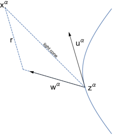
Figure 4: Representation of $z^{\alpha},u^{\alpha}$, $r$, and $w^{\alpha}$.

$$x^{\alpha}=z^{\alpha}(\tau)+r\,\left(u^{\alpha}(\tau)+w^{\alpha}\left(\tau,\theta,\phi\right)\right)\,.$$ (22)

Next, the new coordinates are used to parametrize the Liénard-Wiechert potential $A^{\alpha}$, the field strength tensor $F^{\alpha\beta}=\partial^{\alpha}A^{\beta}-\partial^{\beta}A^{\alpha}$, and the energy-momentum tensor $4\pi T^{\alpha\beta}=F^{\alpha\gamma}F_{\gamma}^{\beta}+\frac{1}{4}\eta^{\alpha\beta}F^{\gamma\delta}F_{\gamma\delta}$. Furthermore, the parameterizations of the tube $V(\tau_{1},\tau_{2})$ and its normal vector $n_{\beta}(x)$ are introduced .

From here on we will use the light-cone coordinates without further notice. For the sake of readability, we will suppress arguments of functions whenever there is no ambiguity. It is understood that fields are evaluated at $x^{\alpha}$, partial derivatives $\partial^{\alpha}$ are meant w.r.t. argument $x^{\alpha}$, and four-vectors derived from the world-line $z^{\alpha}$ of the charge are evaluated at $\tau$.

II.2 The energy-momentum tensor

The Liénard-Wiechert potential is given by

$$A^{\alpha}=q\frac{u^{\alpha}}{r}\,.$$ (23)

In several occasions, for example for the field strength tensor, the derivatives

$$\partial^{\alpha}A^{\beta}=q\left(\frac{a^{\beta}\partial^{\alpha}\tau}{r}-\frac{u^{\beta}\partial^{\alpha}r}{r^{2}}\right)$$ (24)

need to be calculated. Hence,

$$\partial^{\alpha}r=\partial^{\alpha}((x^{\beta}-z^{\beta})u_{\beta})$$

$$=u^{\alpha}+x^{\beta}a_{\beta}\partial^{\alpha}\tau-u^{\beta}u_{\beta}\partial^{\alpha}\tau-z^{\beta}a_{\beta}\partial^{\alpha}\tau$$ (25)

and $\partial^{\beta}\tau$ are needed. The defining relation of the retarded time $(x^{\alpha}-z^{\alpha})(x_{\alpha}-z_{\alpha})=0$ is employed to compute

$$\partial^{\beta}(x^{\alpha}x_{\alpha}-2x^{\alpha}z_{\alpha}+z^{\alpha}z_{\alpha})=0\,,$$ (26)

$$2x^{\beta}-2z^{\beta}-2x^{\alpha}u_{\alpha}\partial^{\beta}\tau+2z^{\alpha}u_{\alpha}\partial^{\beta}\tau=0\,,$$ (27)

$$\partial^{\beta}\tau=\frac{x^{\beta}-z^{\beta}}{(x^{\alpha}-z^{\alpha})u_{\alpha}}=\frac{x^{\beta}-z^{\beta}}{r}=u^{\beta}+w^{\beta}\,.$$ (28)

For the field strength tensor the abbreviation $a^{\alpha}_{\perp}=a^{\alpha}+a^{\beta}w_{\beta}w^{\alpha}$ is used, which is orthogonal to the vectors $u^{\alpha},w^{\alpha}$ implying $a^{\alpha}_{\perp}w_{\alpha}=0$ and $a^{\alpha}_{\perp}u_{\alpha}=0$. The field strength tensor $F^{\alpha\beta}=\partial^{\alpha}A^{\beta}-\partial^{\beta}A^{\alpha}$ is then given by

$$F^{\alpha\beta}= \frac{q}{r^{2}}(w^{\alpha}u^{\beta}-u^{\alpha}w^{\beta})$$ (29)

$$+\frac{q}{r}((u^{\alpha}+w^{\alpha})a^{\beta}_{\perp}-a^{\alpha}_{\perp}(u^{\beta}+w^{\beta}))\,.$$

The first line in (29) is the boosted Coulomb field contribution and the second the radiation field contribution. The associated energy-momentum tensor $4\pi T^{\alpha\beta}=F^{\alpha\gamma}F_{\gamma}^{\beta}+\frac{1}{4}\eta^{\alpha\beta}F^{\gamma\delta}F_{\gamma\delta}$ is given by

$$4\pi T^{\alpha\beta} =\frac{q^{2}}{r^{4}}(u^{\alpha}u^{\beta}-w^{\alpha}w^{\beta}-\frac{1}{2}\eta^{\alpha\beta})$$ (30)

$$+\frac{q^{2}}{r^{3}}(a_{\perp}^{\beta}(u^{\alpha}+w^{\alpha})+a_{\perp}^{\alpha}(u^{\beta}+w^{\beta}))$$

$$-\frac{q^{2}}{r^{2}}a_{\perp}^{\gamma}a_{\perp\gamma}(u^{\alpha}+w^{\alpha})(u^{\beta}+w^{\beta})\,.$$

The derivation of the expressions (22), (29), (30) and the coordinates can be found in Parrott (2012) or Rohrlich (2007).

II.3 Parametrization of the tube $V(\tau_{1},\tau_{2})$ in light cone coordinates

As an introduction we first review how Parrott and Dirac define their tubes. Both use an implicit definition over the lateral surface of their tubes.

The explicit expressions for those 3-dimensional lateral hyper-surfaces is given in terms of the coordinates $\tau,\theta$, and $\phi$, while $\tau_{1}\leq\tau\leq\tau_{2}$. Setting $r=\epsilon$ the lateral surface of Parrott’s tube is obtained

$$t^{\alpha}(\tau,\theta,\phi)=z^{\alpha}(\tau)+\epsilon(u^{\alpha}(\tau)+w^{\alpha}(\tau,\theta,\phi))\,,$$ (31)

which is one of the simplest and at first sight natural choices first employed by Bhabha. The big advantage is that in the limit $\tau_{1}\rightarrow\tau_{2}$ the retarded time $\tau$ for all points on this surface is the same. The disadvantage is that an integration over this area does not lead to a total force, as has been discussed in chapter I.4.

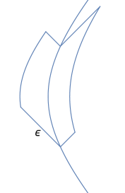
Figure 5: Parrott’s tube, it is defined by moving the length $\epsilon$ along the light cone in all directions between $\tau_{1}$ and $\tau_{2}$.

The lateral surface of Dirac’s tube is given by

$$t^{\alpha}(\tau,\theta,\phi)=z^{\alpha}(\tau)+\epsilon w^{\alpha}(\tau,\theta,\phi)\,.$$ (32)

One has to be careful with the meaning of the argument $\tau$ here, since the retarded time corresponding to some point $t^{\alpha}$ is not $\tau$. This is the case because this representation of the surface does not respect the usual form of light cone coordinates (22). The advantage is, however, that the caps are hyperplanes of simultaneity in the rest frames as necessary for the integration.

The choice of $V(\tau_{1},\tau_{2})$ used in our derivation originates from the ones of Dirac and Parrott. We now parametrize Dirac’s cap at $\tau_{1}$ in such a way that $\tau$ still is the retarded time. An arbitrary point $x^{\alpha}$ lies in the cap if and only if the vector $x^{\alpha}-z^{\alpha}(\tau_{1})$ is orthogonal to the normal vector of the cap. The normal vector is nothing else than $u^{\alpha}(\tau_{1})$. So we demand

$$(x^{\alpha}-z^{\alpha}(\tau_{1}))\,u_{\alpha}(\tau_{1})=0\,.$$ (33)

Next we use the light cone coordinates (22) for $x^{\alpha}$. We follow Parrott’s approach and treat the radius $r$ not as a coordinate but as some function of the coordinates $\tau$, $\theta$, and $\phi$. This leads to the equation

$$(z^{\alpha}+r(u^{\alpha}+w^{\alpha})-z^{\alpha}(\tau_{1}))u_{\alpha}(\tau_{1})=0$$ (34)

for $r$. The result is

$$r=\frac{(z^{\alpha}(\tau_{1})-z^{\alpha})u_{\alpha}(\tau_{1})}{(u^{\alpha}+w^{\alpha})u_{\alpha}(\tau_{1})}\,.$$ (35)

We now have the desired parametrization for the cap

$$c^{\alpha}(\tau,\theta,\phi)=z^{\alpha}+\frac{(z^{\alpha}(\tau_{1})-z^{\alpha})u_{\alpha}(\tau_{1})}{(u^{\alpha}+w^{\alpha})u_{\alpha}(\tau_{1})}(u^{\alpha}+w^{\alpha})\,,$$ (36)

where $\tau_{1}-\epsilon\leq\tau\leq\tau_{1}$. The next step is to find a tube which has such caps. The easiest way is to connect two caps by a smooth transformation. The boundary of the cap at $\tau_{1}$ is defined by $\tau=\tau_{1}-\epsilon$. By shifting $\tau_{1}$ to $\tau_{2}$ the desired hyper-surface is obtained. All that has to be done is to replace $\tau_{1}-\epsilon$ by $\tau$ in (36). With this replacement we get the equation for the tube surface

$$t^{\alpha}(\tau,\theta,\phi)=$$

$$z^{\alpha}+\frac{(z^{\alpha}(\tau+\epsilon)-z^{\alpha})u_{\alpha}(\tau+\epsilon)}{(u^{\alpha}+w^{\alpha})u_{\alpha}(\tau+\epsilon)}(u^{\alpha}+w^{\alpha})\,,$$ (37)

where now $\tau_{1}-\epsilon\leq\tau\leq\tau_{2}-\epsilon$ holds.

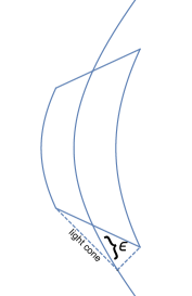
Figure 7: Our tube, it is defined first taking the cut between the hyperplane of simultaneity in the rest frame at $z^{\alpha}(\tau)$ and the forward light cone originating from $z^{\alpha}(\tau-\epsilon)$ and second taking the union of all those cuts between $\tau_{1}$ and $\tau_{2}$.

As a word of caution it has to be mentioned that the definition of the tube surface breaks down for to high accelerations. Hyperplanes of simultaneity in the rest frame at different times always intersect somewhere if the velocities are different at those times. It can happen that this intersection area is closer to the world-line than the radius $\epsilon$ if the acceleration is bigger than $1/\epsilon$ between these times. This is a general phenomenon in special relativity and not specific to our definitions.

The actual calculation of the energy-momentum flow through the tube (II.3) is rather long, so it is given in the appendix V. The flow is obtained by first evaluating an explicit expression for the normal vector on the tube (II.3) and second integrating the contraction of the energy-momentum tensor (30) and the normal vector over tube surface as in (I.1). The next chapter discusses the result of this calculation.

II.4 The new radiation reaction force

The radiation reaction force is given by

$$\partial_{\tau}P^{\alpha}_{\epsilon}(\tau)= -\frac{q^{2}}{6\left[\left(z^{\gamma}-z^{\gamma}(\tau-\epsilon)\right)\,u_{\gamma}\right]^{2}}$$ (38)

$$\left\{\left[u^{\alpha}-4u^{\alpha}(\tau-\epsilon)\,u^{\beta}u_{\beta}(\tau-\epsilon)\right]\right.$$

$$\left.\times\left[1-u^{\delta}u_{\delta}(\tau-\epsilon)+\left(z^{\rho}-z^{\rho}(\tau-\epsilon)\right)\,a_{\rho}\right]\right\}$$

$$-\frac{q^{2}}{6\left(z^{\gamma}-z^{\gamma}(\tau-\epsilon)\right)\,u_{\gamma}}$$

$$\left\{4u^{\alpha}(\tau-\epsilon)\left[a^{\tau}(\tau-\epsilon)\,u_{\tau}+u^{\zeta}(\tau-\epsilon)\,a_{\zeta}\right]\right.$$

$$\left.+4a^{\alpha}(\tau-\epsilon)\,u^{\vartheta}(\tau-\epsilon)\,u_{\vartheta}-a^{\alpha}\right\}$$

$$+\frac{2q^{2}}{3}\,a^{\varphi}(\tau-\epsilon)\,a_{\varphi}(\tau-\epsilon)\,u^{\alpha}(\tau-\epsilon)$$

$$=:L^{\alpha}_{\epsilon}(\tau) \,.$$ (39)

To our knowledge, $L^{\alpha}_{\epsilon}(\tau)$ is the first explicit expression for the radiation reaction force for an extended charged particle in contrast to the approximations in terms of Taylor series in $\epsilon$ which, as we have argued, can be a source dynamical instability.

Nevertheless, it is interesting to perform a Taylor expansion nonetheless in order to see if our expression, at least in lowest orders of $\epsilon$, agrees with the right-hand side of the LAD equation which as found in various computations in the classical literature.

To do this, we make use of $u^{\alpha}u_{\alpha}=1$, $a^{\alpha}u_{\alpha}=0$, and $\dot{a}^{\alpha}u_{\alpha}=-a^{\alpha}a_{\alpha}$. For the terms starting with the first fraction in (38), it is enough to examine the following bracket

$$1-u^{\delta}u_{\delta}(\tau-\epsilon)+(z^{\rho}-z^{\rho}(\tau-\epsilon))\,a_{\rho}=\mathcal{O}(\epsilon^{3})\,.$$ (40)

This fraction does not contribute in the limit $\epsilon\to 0$ term since the nominator is of order $\mathcal{O}(\epsilon^{2})$. The first bracket following the second fraction also does not contribute in this limit since

$$4u^{\alpha}(\tau-\epsilon)\left[a^{\tau}(\tau-\epsilon)\,u_{\tau}+u^{\zeta}(\tau-\epsilon)\,a_{\zeta}\right]=\mathcal{O}(\epsilon^{2})\,.$$ (41)

The remaining terms reduce to the well-known LAD force

$$(\ref{endgl})=- \frac{q^{2}}{6}\Big{(}\frac{4a^{\alpha}(\tau-\epsilon)u^{\vartheta}(\tau-\epsilon)\,u_{\vartheta}-a^{\alpha}}{\left(z^{\gamma}-z^{\gamma}(\tau-\epsilon)\right)\,u_{\gamma}}$$

$$\phantom{\frac{q^{2}}{6}\Big{(}}-4a^{\varphi}(\tau-\epsilon)a_{\varphi}(\tau-\epsilon)u^{\alpha}(\tau-\epsilon)\Big{)}$$

$$= -\frac{q^{2}}{2\epsilon}a^{\alpha}+\frac{2q^{2}}{3}(\dot{a}^{\alpha}+a^{\varphi}a_{\varphi}u^{\alpha})+\mathcal{O}(\epsilon)\,,$$ (42)

which requires a mass renormalization procedure to get rid of the first $O(\epsilon^{-1})$ term by absorbing it into the inertial mass. However, as argued above, this expansion in $\epsilon$ is not helpful for arriving at a sensible dynamics as it is the source of dynamical instabilities.

III Effective equations of motions

In this final chapter we draw from the previously establish result (38) which describes the change of total momentum of our charge distribution. In order to formulate a self-consistent dynamics we still need to establish a relation between this change of momentum and the corresponding change of velocity of the world-line $\tau\mapsto z^{\alpha}(\tau)$. Here, we face the problem that $P^{\alpha}_{\epsilon}(\tau)$ is the total change of momentum of the charge distribution defined by our $\epsilon$-depending tube, as given in Figure 7. In fact, at this point we would need to compute $j_{\epsilon}^{\alpha}(x)$ from (7) and establish the desired relation in view of Dirac’s argument (I.1) by

$$L^{\alpha}_{\epsilon}(\tau)=\partial_{\tau}P_{\epsilon}^{\alpha}(\tau)=\partial_{\tau}\int_{V(\tau_{1},\tau)}d^{4}x\,F^{\alpha\beta}_{\epsilon}(x){j_{\epsilon}}_{\beta}(x).$$ (43)

Note that for point-charges the right-hand side simply reduces to the well-known Lorentz force exerted by the electromagnetic field on the charge; see (I.1). In order to avoid this step we make the following model assumption:

$$P^{\alpha}_{\epsilon}(\tau)=m_{\epsilon}(\tau)\dot{z}^{\alpha}(\tau)$$ (44)

for $m_{\epsilon}(\tau)$ being a proportionality factor that for sake of generality may depend on $\tau$. At this point the explicit dependence on $\tau$ may appear strange, however, it will turn out that this additional degree of freedom will be helpful to arrive at a concept of total inertial mass taking account of the one that is effectively created by the back reaction of the electromagnetic field. By contracting the equality

$$L_{\epsilon}^{\alpha}(\tau)=\partial_{t}m_{\epsilon}(\tau)\dot{z}^{\alpha}(\tau)+m_{\epsilon}(\tau)\ddot{z}^{\alpha}(\tau)$$ (45)

with $\dot{z}_{\alpha}(\tau)$ and, exploiting $\dot{z}_{\alpha}(\tau)\,\dot{z}^{\alpha}(\tau)=1$ and $\dot{z}_{\alpha}(\tau)\,\ddot{z}^{\alpha}(\tau)=0$, we infer

$$\partial_{t}m_{\epsilon}(\tau)=L^{\alpha}_{\epsilon}(\tau)\dot{z}_{\alpha}(\tau)\,.$$ (46)

Defining the relativistic force

$$F_{\epsilon}^{\alpha}(\tau):=L^{\alpha}_{\epsilon}(\tau)-\dot{z}^{\alpha}L_{\epsilon}^{\beta}(\tau)\dot{z}_{\beta}(\tau)$$ (47)

that is four-orthogonal to $\dot{z}^{\alpha}(\tau)$, we arrive at the dynamical system

$$\frac{d}{d\tau}\begin{pmatrix}z^{\alpha}_{\epsilon}(\tau)\\ u^{\alpha}_{\epsilon}(\tau)\\ m_{\epsilon}(\tau)\end{pmatrix}=\begin{pmatrix}u^{\alpha}_{\epsilon}(\tau)\\ \frac{1}{m_{\epsilon}(\tau)}\,\left(F^{\alpha}_{\epsilon}[z](\tau)+F^{\alpha}_{\text{ext}}(\tau)\right)\\ {u_{\epsilon}}_{\alpha}(\tau)L^{\alpha}_{\epsilon}[z](\tau)\end{pmatrix}\,,$$ (48)

where for the discussion below we introduced an additional external force $F^{\alpha}_{\text{ext}}(\tau)$ acting on the charge that is four-orthogonal to $\dot{z}^{\alpha}(\tau)$. This system couples the world-line $\tau\mapsto z^{\alpha}(\tau)$ to the change of momentum computed in (38) caused by the electromagnetic field that, in turn, is produced by the charge itself. Here, the argument $[z]$ in square brackets is to remind us that these terms are functionals of the world-line $t\mapsto z^{\alpha}(\tau)$. In fact, inspecting the expression (38) reveals that the system (48) effectively turns out to be a system non-linear and neutral delay equations. The delay stems form the fact that the charge has the extension of our $\epsilon$ tube and the speed of light is finite and is therefore expected. Note that the initial value of the proportionality factor $m(0)$ is an additional degree of freedom. Based on the general theory of delay equations, it is to be expected that the initial values of this system are twice continuously differentiable trajectory strips $z^{\alpha}:[-\epsilon,0]\to\mathbb{R}^{4}$ together with the value $m_{\epsilon}(0)\in\mathbb{R}$.

To understand this system of equations (48) better, we consider the simple case of an external force $F^{\alpha}_{\text{ext}}$ that is tuned to force the charge into an uniform acceleration, say, along the $z$-coordinate for $\tau\in\Lambda$. If it was not for the expected radiation reaction force we are interested in, this setting could be thought of a charge in a constant electric field. Here, however, it is important to keep in mind that the considered external force also compensates possible friction, e.g., due to the radiation reaction, to keep the acceleration constant. In this case the world-line is given by

$$z^{\alpha}(\tau)=\frac{1}{g}\,\left(\sinh(g\tau),0,0,\cosh(g\tau)\right)\,,$$ (49)

where $g$ is the constant acceleration on the interval $\tau\in\Lambda$. The change in momentum due to the back reaction, computed from (38), has the correspondingly simple form

$$L_{\epsilon}^{\alpha}(\tau)=-\frac{q^{2}g}{2\sinh(g\epsilon)}\,a^{\alpha}(\tau)$$ (50)

for $\tau\in\Lambda$. In view of the equation of motion (48) we obtain $\dot{m}_{\epsilon}(\tau)=0$, and hence,

$$\left(m_{\epsilon}(0)+\frac{q^{2}g}{2\sinh(g\epsilon)}\right)a^{\alpha}(\tau)=F^{\alpha}_{\text{ext}}(\tau)\,,$$ (51)

which gives rise to the following total inertial mass when measured w.r.t. the external force:

$$m_{\text{tot}}=m_{\epsilon}(0)+\frac{q^{2}g}{2\sinh(g\epsilon)}\,.$$ (52)

Two properties of (52) can be observed: First, as in (42), the correction to the inertia originating from the electromagnetic field in leading order as $\epsilon\to 0$ equals $q^{2}/2\epsilon$:

$$m_{\text{tot}}=m_{\epsilon}(0)+\frac{q^{2}}{2\epsilon}-\frac{q^{2}g^{2}}{12}\,\epsilon+O(\epsilon^{2})\,.$$ (53)

And second, the higher-order corrections in (53) explicitly depend on the dynamics itself, in this case on the acceleration parameter $g$. To illustrate the dependence on the dynamics even more clearly, we consider eigentimes $0<\tau_{1}<\tau_{2}$ with $\tau_{2}-\tau_{1}>2\epsilon$ and define $\Lambda_{1}=[0,\tau_{1})$, $\Lambda=[\tau_{1},\tau_{2})$, and $\Lambda_{2}=[\tau_{2},+\infty)$. We assume that the external force $F^{\alpha}_{\text{ext}}$ is tuned such that the effective acceleration in $\Lambda_{1}\cup[\tau_{1},\tau_{1}+\epsilon)$ and $[\tau_{2}-\epsilon)\cup\Lambda_{2}$ is constant and equal to $g_{1}$ and $g_{2}$, respectively, where $g_{1}\neq g_{2}$. Furthermore, we assume that in the intermediate interval $[\tau_{1}+\epsilon,\tau_{2}-\epsilon)$ the acceleration of the charge changes smoothly from $g_{1}$ to $g_{2}$ obeying $\dot{m}_{\epsilon}(\tau)=0$ for $\tau\in\Lambda$. By virtue of (48) we observe that

$$z_{i}^{\alpha}(\tau) =\frac{1}{g_{i}}\,\left(\sinh(g_{i}\tau),0,0,\cosh(g_{i}\tau)\right)\quad\text{for }\tau\in\Lambda_{i}$$ (54)

solves (48) for $i=1,2$ which, by (52), implies that the corresponding total inertial mass $m_{\text{tot}}$ depends on the eigentime $\tau$, more precisely it holds

$$m_{\text{tot}}=m_{\epsilon}(0)+\begin{cases}\frac{q^{2}g_{1}}{2\sinh(g_{1}\epsilon)}\quad\text{for }\tau\in\Lambda_{1}\\ \frac{q^{2}g_{2}}{2\sinh(g_{2}\epsilon)}\quad\text{for }\tau\in\Lambda_{2}\end{cases}\,.$$ (55)

It is therefore to be expected that the total inertial mass is a dynamical quantity. The concept of a time-dependent total inertial mass is not new but also observed in other theories treating back-reaction, e.g., in Bopp-Podolski’s generalized electrodynamics Zayats (2014). For our system (48) the time-dependency is foremost due to the time-dependent shape of our $\epsilon$ tube.

IV Conclusion

Whether $\epsilon$ is kept finite or a limit $\epsilon\to 0$ is considered, in our approach the inertial mass is an emerging phenomenon that originates from the back reaction on the charge exerted by its own electromagnetic field. Thus, a general procedure is needed to gauge the inertial mass to the one observed in the experiment. In view of (53), the renormalization procedure $m_{\epsilon}(0)=m_{\text{exp}}-q^{2}/2\epsilon$ for $m_{\text{exp}}$ being the experimentally measured inertial mass, as also employed by Dirac, is appropriate as long as the time-dependent terms are subleading. However, we emphasize again that the higher-order terms in (53) may not simply be neglected in a limiting procedure $\epsilon\to 0$ as the Taylor expansion of solutions $z^{\alpha}(\tau)$ on the right-hand side of the equations of motion (48) cannot be controlled uniformly on time intervals. The neglect of higher-order terms may provoke the so-called runaway solutions as illustrated with the counter example given in Section I.3. The virtue of our approach is therefore that no Taylor expansion has been employed when formulating the law of motion (48). Instead we are left with an explicit expression (38) that can readily be studied analytically or numerically in various settings. One imminent question is whether the dynamical system (48) is stable and does in particular not lead to the notorious run-away solutions. A thorough analysis of this question is left for a forthcoming paper.

The only assumptions involved in the derivation of system (48) were:

1. Energy-momentum conservation between the kinetic and the field degrees of freedom as expressed in differential form in change of momentum as given by (43).

2. The special form of the $\epsilon$-tube that allowes the explicit evaluation of the integrals involved in computing the momentum change in Section V.2.

3. The assumption (44) that allows to relate the change of momentum to the change of velocity which is a pathology of the extended charge model.

While assumption 1. seems rather natural, assumption 2. arises out of the mathematical necessity to introduce a cut-off in the electromagnetic fields as the solutions of the Maxwell equations are ill-defined on the world-line for point-charges. Of course, in other settings, as the above mentioned generalized electrodynamics, this point can potentially be avoided at the cost of replacing Maxwell’s equations with a more regular version of the latter. This may be a valid approach but is not our focus here. Moreover, one may wonder, how much information of the particular shape of the employed $\epsilon$-tube enters the law of motion (48). In view of the Stoke’s theorem employed in the derivation of the momentum change, recall (I.1), only the geometric properties of the caps of the tube enter in expression (38). Assumption 3. is certainly the most ad hoc one. Indeed, a more subtle analysis of (43) is required to argue for the validity of the given approximation (44) in a certain regime. However, this goes beyond the scope of this work. Furthermore, the explicit form of the law of motion (48) allows the exploration of example settings, such as the synchrotron setting, in which a charge moves in a constant magnetic field perpendicular to the motion, for which already other approaches, such as the Landau-Lifschitz equations, make predictions. Based on an understanding in these settings, a sensible renormalisation procedure has to be developed. It is our hope that the additional degree of freedom in $m_{\epsilon}(\tau)$ can compensate the time-dependencies of our $\epsilon$-tube to some extend so that in a regime of sufficiently small $\epsilon$ the renormalised solutions to (48) become rather independent of the cut-off. Both of these open points will be addressed in a follow-up article which is in preparation.

V Appendix: Computation of the force

V.1 The normal vector on the tube

The direct way to calculate the normal vector $n^{\alpha}$ is to make use of the fact that there exists only one unit vector which is orthogonal to all the tangent vectors of the tube $t^{\alpha}$ up to the sign. The three tangent vectors are given by the derivatives of $t^{\alpha}$ with respect to $\tau$, $\theta$, and $\phi$. The contraction of those three vectors with the epsilon tensor gives a vector which is automatically orthogonal to the tangent vectors. In some sense the epsilon tensor is the generalization of the cross product to higher dimensions. In the language of differential geometry, the normal vector $n^{\alpha}$ is the hodge dual of the wedge product of the tangent vectors. It follows that the normal vector $n^{\alpha}$ is given by

$$n^{\alpha}=\epsilon^{\alpha\beta\gamma\delta}\,\partial_{\tau}t_{\beta}\,\partial_{\theta}t_{\gamma}\,\partial_{\phi}t_{\delta}\,.$$ (56)

Its length is the volume spanned by a unit normal vector and the three tangent vectors, which is nothing else than the Jacobian determinant. Hence, we do not even need to adjust it. The tangent vectors are

$$\partial_{\tau}t^{\alpha}=u^{\alpha}+\partial_{\tau}r(u^{\alpha}+w^{\alpha})+r(a^{\alpha}+\partial_{\tau}w^{\alpha})\,,$$ (57)

$$\partial_{\theta}t^{\alpha}=\partial_{\theta}r(u^{\alpha}+w^{\alpha})+r(\partial_{\theta}w^{\alpha})\,,$$ (58)

$$\partial_{\phi}t^{\alpha}=\partial_{\phi}r(u^{\alpha}+w^{\alpha})+r(\partial_{\phi}w^{\alpha})\,.$$ (59)

The derivatives of r are lengthy expressions. So it makes sense not to calculate a complete expression for the normal vector but instead state only its components in an useful orthonormal basis. For this basis we choose

$$u^{\alpha}\,,\quad w^{\alpha}\,,\quad\theta^{\alpha}=\partial_{\theta}w^{\alpha}\,,\quad\phi^{\alpha}=\frac{\partial_{\phi}w^{\alpha}}{\sin\theta}$$ (60)

and

$$n^{\alpha}=n^{\beta}u_{\beta}u^{\alpha}-n^{\beta}w_{\beta}w^{\alpha}$$

$$\hskip 56.9055pt-n^{\beta}\theta_{\beta}\theta^{\alpha}-n^{\beta}\phi_{\beta}\phi^{\alpha}\,.$$ (61)

We start with the term $n^{\beta}u_{\beta}$ on the right-hand side of (V.1) which yields

$$n_{\delta}u^{\delta} = \epsilon_{\alpha\beta\gamma\delta}\partial_{\tau}t^{\alpha}\partial_{\theta}t^{\beta}\partial_{\phi}t^{\gamma}u^{\delta}$$ (62)

$$= \begin{vmatrix}1+\partial_{\tau}r-ra^{\beta}w_{\beta}&\partial_{\theta}r&\partial_{\phi}r&1\\ \partial_{\tau}r-ra^{\beta}w_{\beta}&\partial_{\theta}r&\partial_{\phi}r&0\\ -ra^{\beta}\theta_{\beta}-r\partial_{\tau}w^{\beta}\theta_{\beta}&r&0&0\\ -ra^{\beta}\phi_{\beta}-r\partial_{\tau}w^{\beta}\phi_{\beta}&0&\sin\theta\,r&0\end{vmatrix}$$

$$= -(r^{2}\sin\theta\,(\partial_{\tau}r-ra^{\beta}w_{\beta})$$

$$+r^{2}\partial_{\phi}r(a^{\beta}\phi_{\beta}+\partial_{\tau}w^{\beta}\phi_{\beta})$$

$$+r^{2}\sin\theta\,\partial_{\theta}r(a^{\beta}\theta_{\beta}+\partial_{\tau}w^{\beta}\theta_{\beta}))\,,$$

where use has been made of $u^{\alpha}w_{\alpha}=0$ leading to $u^{\alpha}\partial_{\tau}w_{\alpha}=-a^{\alpha}w_{\alpha}$. To obtain the term $n^{\beta}w_{\beta}$ in (V.1) the $1$ showing up in the last column of the determinant in (62) has to shifted down by one row. This yields

$$n_{\alpha}w^{\alpha} = r^{2}\sin\theta\,(1+\partial_{\tau}r-ra^{\beta}w_{\beta})$$ (63)

$$+r^{2}\partial_{\phi}r(a^{\beta}\phi_{\beta}+\partial_{\tau}w^{\beta}\phi_{\beta})$$

$$+r^{2}\sin\theta\,\partial_{\theta}r(a^{\beta}\theta_{\beta}+\partial_{\tau}w^{\beta}\theta_{\beta})\,.$$

The contractions of $n_{\alpha}$ with $\theta^{\alpha}$ and $\phi^{\alpha}$ are obtained in the same way by shifting the $1$ further down. This gives

$$n_{\alpha}\theta^{\alpha}=-r\sin\theta\,\partial_{\theta}r\,,$$ (64)

$$n_{\alpha}\phi^{\alpha}=-r\partial_{\phi}r\,.$$ (65)

The derivatives of the radius in (II.3) are given by

$$\partial_{\tau}r = \Big{(}\big{[}(u^{\alpha}(\tau+\epsilon)-u^{\alpha})\,u_{\alpha}(\tau+\epsilon)$$ (66)

$$\hskip 28.45274pt+(z^{\alpha}(\tau+\epsilon)-z^{\alpha})\,a_{\alpha}(\tau+\epsilon)\big{]}$$

$$\hskip 85.35826pt\times\left(u^{\beta}+w^{\beta}\right)\,u_{\beta}(\tau+\epsilon)$$

$$-\left(z^{\beta}(\tau+\epsilon)-z^{\beta}\right)\,u_{\beta}(\tau+\epsilon)$$

$$\hskip 28.45274pt\times\big{[}\left(a^{\alpha}+\partial_{\tau}w^{\alpha}\right)\,u_{\alpha}(\tau+\epsilon)$$

$$\hskip 56.9055pt+\left(u^{\alpha}+w^{\alpha}\right)\,a_{\alpha}(\tau+\epsilon)\big{]}\Big{)}$$

$$/\big{[}\left(u^{\alpha}+w^{\alpha}\right)\,u_{\alpha}(\tau+\epsilon)\big{]}^{2}\,,$$

$$\partial_{\theta}r = -\left(z^{\alpha}(\tau+\epsilon)-z^{\alpha}\right)\,u_{\alpha}(\tau+\epsilon)$$ (67)

$$\hskip 28.45274pt\times\left[\partial_{\theta}w^{\beta}\,u_{\beta}(\tau+\epsilon)\right]$$

$$/\big{[}\left(u^{\alpha}+w^{\alpha}\right)\,u_{\alpha}(\tau+\epsilon)\big{]}^{2}\,,$$

$$\partial_{\phi}r = -\left(z^{\alpha}(\tau+\epsilon)-z^{\alpha}\right)\,u_{\alpha}(\tau+\epsilon)$$ (68)

$$\hskip 28.45274pt\times\left[\partial_{\phi}w^{\beta}\,u_{\beta}(\tau+\epsilon)\right]$$

$$/\big{[}(u^{\alpha}+w^{\alpha})\,u_{\alpha}(\tau+\epsilon)\big{]}^{2}\,.$$

Now the contraction of the energy-momentum tensor (30) with the normal vector $n^{\alpha}$ can be calculated. The corresponding calculations and integrations are carried out in the next section.

V.2 Computation of the change of the momentum

We start with (I.1) and the domain of (II.3) to obtain

$$\partial_{\tau}P^{\alpha}_{\epsilon}(\tau) = -\partial_{\tau}\int_{\partial V(\tau_{1},\tau)}d^{3}x_{\beta}T^{\alpha\beta}_{\epsilon}$$ (69)

$$= -\partial_{\tau}\int_{\tau_{1}-\epsilon}^{\tau-\epsilon}d\tau\int_{0}^{\pi}d\theta\int_{0}^{2\pi}d\phi\,n_{\beta}\,T^{\alpha\beta}\,.$$

In the following we also consider the integral domains given in (69) and suppress their reference in our notation. Due to the cut-off, the cap integrals vanish since $T^{\alpha\beta}_{\epsilon}=0$ within the tube and only the integral over the lateral surface of the tube remains, where $T^{\alpha\beta}_{\epsilon}=T^{\alpha\beta}$ holds. First the angle integration is performed and also a factor of $4\pi/q^{2}$ is introduced for convenience. To carry out the calculations, we make use of $\eta^{\alpha\beta}=u^{\alpha}u^{\beta}-w^{\alpha}w^{\beta}-\theta^{\alpha}\theta^{\beta}-\phi^{\alpha}\phi^{\beta}$ and (30) for $T^{\alpha\beta}$ and (62)-(65) for $n_{\beta}$. This leads to

$$\int d\theta d\phi\,n_{\beta}\,\frac{4\pi}{q^{2}}T^{\alpha\beta}$$

$$=\int d\theta d\phi\,n_{\beta}\,\Big{[}\frac{u^{\alpha}u^{\beta}-w^{\alpha}w^{\beta}+\theta^{\alpha}\theta^{\beta}+\phi^{\alpha}\phi^{\beta}}{2r^{4}}+\frac{a_{\perp}^{\beta}(u^{\alpha}+w^{\alpha})+a_{\perp}^{\alpha}(u^{\beta}+w^{\beta})}{r^{3}}-\frac{a_{\perp}^{\gamma}a_{\perp\gamma}\left(u^{\alpha}+w^{\alpha}\right)\left(u^{\beta}+w^{\beta}\right)}{r^{2}}\Big{]}$$

$$=\int\,d\theta d\phi\,\left(\overbrace{\frac{-u^{\alpha}\sin\theta\,}{2r^{2}}\partial_{\tau}r}^{i}-\overbrace{\frac{w^{\alpha}\sin\theta\,}{2r^{2}}\partial_{\tau}r}^{ii}+\overbrace{\frac{u^{\alpha}\sin\theta\,}{2r}a^{\beta}w_{\beta}}^{iii}+\overbrace{\frac{w^{\alpha}\sin\theta\,}{2r}a^{\beta}w_{\beta}}^{iv}-\overbrace{\frac{w^{\alpha}\sin\theta\,}{2r^{2}}}^{v}-\overbrace{\frac{u^{\alpha}}{2r^{2}}a^{\beta}\phi_{\beta}\partial_{\phi}r}^{via}\right.$$

$$\hskip 56.9055pt-\overbrace{\frac{u^{\alpha}\sin\theta\,}{2r^{2}}a^{\beta}\theta_{\beta}\partial_{\theta}r}^{vib}-\overbrace{\frac{w^{\alpha}}{2r^{2}}a^{\beta}\phi_{\beta}\partial_{\phi}r}^{viia}-\overbrace{\frac{w^{\alpha}\sin\theta\,}{2r^{2}}a^{\beta}\theta_{\beta}\partial_{\theta}r}^{viib}-\overbrace{\frac{u^{\alpha}}{2r^{2}}\partial_{\tau}w^{\beta}\phi_{\beta}\partial_{\phi}r}^{viiia}-\overbrace{\frac{u^{\alpha}\sin\theta\,}{2r^{2}}\partial_{\tau}w^{\beta}\theta_{\beta}\partial_{\theta}r}^{viiib}$$

$$\hskip 85.35826pt-\overbrace{\frac{w^{\alpha}}{2r^{2}}\partial_{\tau}w^{\beta}\phi_{\beta}\partial_{\phi}r}^{ixa}-\overbrace{\frac{w^{\alpha}\sin\theta\,}{2r^{2}}\partial_{\tau}w^{\beta}\theta_{\beta}\partial_{\theta}r}^{ixb}-\overbrace{\frac{\sin\theta\,\theta^{\alpha}}{2r^{3}}\partial_{\theta}r}^{xa}-\overbrace{\frac{\phi^{\alpha}}{2r^{3}}\partial_{\phi}r}^{xb}+\overbrace{\frac{\sin\theta\,a^{\alpha}_{\perp}}{r}}^{xi}$$

$$\left.\hskip 142.26378pt+\overbrace{\frac{\sin\theta\,(u^{\alpha}+w^{\alpha})}{r^{2}}a^{\beta}\theta_{\beta}\partial_{\theta}r}^{xiia}+\overbrace{\frac{u^{\alpha}+w^{\alpha}}{r^{2}}a^{\beta}\phi_{\beta}\partial_{\phi}r}^{xiib}-\overbrace{a_{\perp}^{\gamma}a_{\perp\gamma}(u^{\alpha}+w^{\alpha})\sin\theta}^{xiii}\right)\,.$$ (70)

As is seen from (V.2) only angle integrations remain to be carried out. Since the integral (V.2) is a Lorentz vector the integrations can be carried out in the rest frame. The original expressions are then obtained by transforming back to lab frame. It is worth noting that only the vectors $w^{\alpha}$, $\theta^{\alpha}$, and $\phi^{\alpha}$ depend on the angles $\theta$ and $\phi$. The quantities $\theta^{\alpha}$ and $\phi^{\alpha}$ only appear in the combination $\theta^{\alpha}\theta^{\beta}+\phi^{\alpha}\phi^{\beta}$. In the rest frame

$$\theta_{0}^{\alpha}\theta_{0}^{\beta}+\phi_{0}^{\alpha}\phi_{0}^{\beta}=m^{\alpha\beta}-w_{0}^{\alpha}w^{\beta}_{0}$$ (71)

holds, where

$$m^{\alpha\beta}=\begin{pmatrix}0&0&0&0\\ 0&1&0&0\\ 0&0&1&0\\ 0&0&0&1\\ \end{pmatrix}\,,\quad w^{\alpha}_{0}=\begin{pmatrix}0\\ \sin\theta\,\cos\phi\,\\ \sin\theta\,\sin\phi\,\\ \cos\theta\end{pmatrix}\,.$$ (72)

Making use of (71) and pulling angle independent terms out of the integrals in (V.2), all remaining terms are only integrals over powers of $w^{\alpha}_{0}$. The following integrals are needed:

$$\int d\theta d\phi\,\sin\theta=4\pi\,,$$ (73)

$$\int d\theta d\phi\,w_{0}^{\alpha}\sin\theta=0\,,$$ (74)

$$\int d\theta d\phi\,w_{0}^{\alpha}w_{0}^{\beta}\sin\theta=\frac{4\pi}{3}m^{\alpha\beta}\,,$$ (75)

$$\int d\theta d\phi\,w_{0}^{\alpha}w_{0}^{\beta}w_{0}^{\gamma}\sin\theta=0\,,$$ (76)

$$\int d\theta d\phi\,w_{0}^{\alpha}w_{0}^{\beta}w_{0}^{\gamma}w_{0}^{\delta}\sin\theta$$

$$=\frac{4\pi}{15}\left(m^{\alpha\beta}m^{\gamma\delta}+m^{\alpha\gamma}m^{\beta\delta}+m^{\alpha\delta}m^{\gamma\beta}\right)\,.$$ (77)

The transformation of $m^{\alpha\beta}$ back to the lab frame is what remains to be done. To determinate the necessary Lorentz matrix $\Lambda^{\alpha}_{\beta}$ we make use of

$$m^{\alpha\beta}=\delta^{\alpha}_{0}\delta^{\beta}_{0}-\eta^{\alpha\beta}$$ (78)

and $\Lambda^{\alpha}_{0}=\Lambda^{0}_{\alpha}=u^{\alpha}$. We obtain

$$\Lambda^{\alpha}_{\gamma}m^{\gamma\delta}\Lambda_{\delta}^{\beta}$$

$$=\Lambda^{\alpha}_{\gamma}\,\left(\delta^{\gamma}_{0}\delta^{\delta}_{0}-\eta^{\gamma\delta}\right)\,\Lambda_{\delta}^{\beta}$$

$$=u^{\alpha}u^{\beta}-\eta^{\alpha\beta}\,.$$ (79)

With the help of (73) to (77) and (V.2), the integrations $\framebox{i}-\framebox{xiii}$ in (V.2) are straight forward. We obtain for integral i

i $$= \int d\theta d\phi\,\frac{-\sin\theta\,u^{\alpha}}{2r^{2}}\,\partial_{\tau}r$$ (80)

$$= \int d\theta d\phi\,\frac{-\sin\theta\,u^{\alpha}}{2\left[(z^{\gamma}(\tau+\epsilon)-z^{\gamma})\,u_{\gamma}(\tau+\epsilon)\right]^{2}}$$

$$\left(\left[1-u^{\delta}u_{\delta}(\tau+\epsilon)+\left(z^{\mu}(\tau+\epsilon)-z^{\mu}\right)\,a_{\mu}(\tau+\epsilon)\right]\right.$$

$$\left(u^{\beta}+w^{\beta}\right)\,u_{\beta}(\tau+\epsilon)-\left(z^{\nu}(\tau+\epsilon)-z^{\nu}\right)\,u_{\nu}(\tau+\epsilon)\,$$

$$\left.\left[\left(a^{\lambda}+\partial_{\tau}w^{\lambda}\right)\,u_{\lambda}(\tau+\epsilon)+\left(u^{\kappa}+w^{\kappa}\right)\,a_{\kappa}(\tau+\epsilon)\right]\right)$$

$$= \frac{-2\pi u^{\alpha}}{\left[\left(z^{\gamma}(\tau+\epsilon)-z^{\gamma}\right)\,u_{\gamma}(\tau+\epsilon)\right]^{2}}$$

$$\left(\left[1-u^{\delta}u_{\delta}(\tau+\epsilon)+\left(z^{\mu}(\tau+\epsilon)-z^{\mu}\right)\,a_{\mu}(\tau+\epsilon)\right]\right.$$

$$u^{\beta}u_{\beta}(\tau+\epsilon)-\left(z^{\nu}(\tau+\epsilon)-z^{\nu}\right)\,u_{\nu}(\tau+\epsilon)$$

$$\left.\left[a^{\lambda}u_{\lambda}(\tau+\epsilon)+u^{\kappa}a_{\kappa}(\tau+\epsilon)\right]\right)\,.$$

For integral ii, we obtain

ii $$= \int d\theta d\phi\,\frac{-\sin\theta\,w^{\alpha}}{2r^{2}}\,\partial_{\tau}r$$ (81)

$$= \int d\theta d\phi\,\frac{-\sin\theta\,w^{\alpha}}{2\left[\left(z^{\gamma}(\tau+\epsilon)-z^{\gamma}\right)\,u_{\gamma}(\tau+\epsilon)\right]^{2}}$$

$$\left(\left[1-u^{\delta}u_{\delta}(\tau+\epsilon)+\left(z^{\mu}(\tau+\epsilon)-z^{\mu}\right)\,a_{\mu}(\tau+\epsilon)\right]\right.$$

$$\left(u^{\beta}+w^{\beta}\right)\,u_{\beta}(\tau+\epsilon)-\left(z^{\lambda}(\tau+\epsilon)-z^{\lambda}\right)\,u_{\lambda}(\tau+\epsilon)\,$$

$$\left.\left[\left(a^{\kappa}+\partial_{\tau}w^{\kappa}\right)\,u_{\kappa}(\tau+\epsilon)+\left(u^{\nu}+w^{\nu}\right)\,a_{\nu}(\tau+\epsilon)\right]\right)$$

$$= \frac{-2\pi}{3\left[\left(z^{\gamma}(\tau+\epsilon)-z^{\gamma}\right)\,u_{\gamma}(\tau+\epsilon)\right]^{2}}$$

$$\left(\vphantom{\Lambda^{\gamma}_{\delta}\,\Lambda^{\alpha}_{\mu}\,m^{\delta\mu}}\left[1-u^{\delta}u_{\delta}(\tau+\epsilon)+\left(z^{\mu}(\tau+\epsilon)-z^{\mu}\right)\,a_{\mu}(\tau+\epsilon)\right]\right.$$

$$\hskip 28.45274ptu_{\beta}(\tau+\epsilon)\,\left(u^{\alpha}u^{\beta}-\eta^{\alpha\beta}\right)$$

$$-\left(z^{\lambda}(\tau+\epsilon)-z^{\lambda}\right)\,u_{\lambda}(\tau+\epsilon)$$

$$\hskip 28.45274pt\left[a_{\nu}(\tau+\epsilon)\,\left(u^{\alpha}u^{\nu}-\eta^{\alpha\nu}\right)\right.$$

$$\left.\left.\hskip 56.9055pt+u_{\kappa}(\tau+\epsilon)\,\partial_{\tau}\Lambda^{\kappa}_{\rho}\,\Lambda^{\alpha}_{\chi}\,m^{\rho\chi}\right]\right)\,.$$

To simplify (81) further we need an expression for $\partial_{\tau}\Lambda^{\kappa}_{\rho}\,\Lambda^{\alpha}_{\chi}\,m^{\rho\chi}$. With the help of (78) for $m^{\alpha\beta}$ this yields $a^{\gamma}u^{\alpha}$ for the term that contains the two Kronecker deltas. To evaluate the term containing $\eta^{\alpha\beta}$ we go into the co-moving frame. The required Lorentz matrix is just a unit matrix while its derivative contains only accelerations in the time-space part as can be understood by considering the non-relativistic limit. We find

$$\partial_{\tau}\Lambda^{\gamma}_{\delta}\,\Lambda^{\alpha}_{\mu}\,\eta^{\delta\mu} = \begin{pmatrix}0&-a^{1}&-a^{2}&-a^{3}\\ a^{1}&0&0&0\\ a^{2}&0&0&0\\ a^{3}&0&0&0\\ \end{pmatrix}$$ (82)

$$= a^{\gamma}u^{\alpha}-a^{\alpha}u^{\gamma}\,.$$

We note that in the rest frame the well-know Thomas precession is absent. With both terms combined we get $\partial_{\tau}\Lambda^{\gamma}_{\delta}\,\Lambda^{\alpha}_{\mu}\,m^{\delta\mu}=u^{\gamma}a^{\alpha}$. For integral iii we obtain

iii $$= \int d\theta d\phi\,\frac{\sin\theta\,u^{\alpha}}{2r}a^{\beta}w_{\beta}$$ (83)

$$= \int d\theta d\phi\,\frac{\sin\theta\,u^{\alpha}\left(u^{\delta}+w^{\delta}\right)\,u_{\delta}(\tau+\epsilon)\,a^{\beta}w_{\beta}}{2\left(z^{\gamma}(\tau+\epsilon)-z^{\gamma}\right)\,u_{\gamma}(\tau+\epsilon)}$$

$$= \frac{2\pi u^{\alpha}\,u_{\delta}(\tau+\epsilon)\,a_{\beta}\left(u^{\beta}u^{\delta}-\eta^{\beta\delta}\right)}{3\left(z^{\gamma}(\tau+\epsilon)-z^{\gamma}\right)\,u_{\gamma}(\tau+\epsilon)}$$

$$= \frac{-2\pi u^{\alpha}\,u_{\delta}(\tau+\epsilon)\,a^{\delta}}{3\left(z^{\gamma}(\tau+\epsilon)-z^{\gamma}\right)\,u_{\gamma}(\tau+\epsilon)}\,,$$

while integral iv can be recast into

iv $$= \int d\theta d\phi\,\frac{\sin\theta\,w^{\alpha}}{2r}\,a^{\beta}w_{\beta}$$ (84)

$$= \int d\theta d\phi\,\frac{\sin\theta\,w^{\alpha}\left(u^{\delta}+w^{\delta}\right)\,u_{\delta}(\tau+\epsilon)\,a^{\beta}w_{\beta}}{2\left(z^{\gamma}(\tau+\epsilon)-z^{\gamma}\right)\,u_{\gamma}(\tau+\epsilon)}$$

$$= \frac{2\pi\,u^{\delta}u_{\delta}(\tau+\epsilon)\,a_{\beta}\left(u^{\alpha}u^{\beta}-\eta^{\alpha\beta}\right)}{3\left(z^{\gamma}(\tau+\epsilon)-z^{\gamma}\right)\,u_{\gamma}(\tau+\epsilon)}$$

$$= \frac{-2\pi\,a^{\alpha}\,u^{\delta}u_{\delta}(\tau+\epsilon)}{3\left(z^{\gamma}(\tau+\epsilon)-z^{\gamma}\right)\,u_{\gamma}(\tau+\epsilon)}\,.$$

Integrals v and via give

v $$= \int d\theta d\phi\,\frac{-\sin\theta\,w^{\alpha}}{2r^{2}}$$ (85)

$$= \int d\theta d\phi\,\frac{-\sin\theta\,w^{\alpha}\left[\left(u^{\beta}+w^{\beta}\right)\,u_{\beta}(\tau+\epsilon)\right]^{2}}{2\left[\left(z^{\gamma}(\tau+\epsilon)-z^{\gamma}\right)\,u_{\gamma}(\tau+\epsilon)\right]^{2}}$$

$$= \frac{-4\pi\,u^{\beta}u_{\beta}(\tau+\epsilon)\,u_{\delta}(\tau+\epsilon)\,\left(u^{\alpha}u^{\delta}-\eta^{\alpha\delta}\right)}{3\left[\left(z^{\gamma}(\tau+\epsilon)-z^{\gamma}\right)\,u_{\gamma}(\tau+\epsilon)\right]^{2}}$$

and

via $$= \int d\theta d\phi\,\frac{-u^{\alpha}}{2r^{2}}\,\partial_{\phi}r\,a^{\beta}\phi_{\beta}$$ (86)

$$= \int d\theta d\phi\,\frac{u^{\alpha}\sin\theta\,\phi^{\delta}\,u_{\delta}(\tau+\epsilon)\,a^{\beta}\phi_{\beta}}{2\left(z^{\gamma}(\tau+\epsilon)-z^{\gamma}\right)\,u_{\gamma}(\tau+\epsilon)}\,.$$

Integral vib can be evaluated similarly, only $\phi^{\alpha}$ and $\theta^{\alpha}$ are exchanged. Integrals via and vib yield together

$$\framebox{via}+\framebox{vib}$$ (87)

$$= \frac{u^{\alpha}\,u_{\delta}(\tau+\epsilon)\,a_{\beta}}{2\left(z^{\gamma}(\tau+\epsilon)-z^{\gamma}\right)\,u_{\gamma}(\tau+\epsilon)}$$

$$\left[4\pi\,\left(u^{\beta}u^{\delta}-\eta^{\beta\delta}\right)-\frac{4\pi}{3}\left(u^{\beta}u^{\delta}-\eta^{\beta\delta}\right)\right]$$

$$= \frac{-4\pi\,u^{\alpha}\,u_{\delta}(\tau+\epsilon)\,a^{\delta}}{3\left(z^{\gamma}(\tau+\epsilon)-z^{\gamma}\right)\,u_{\gamma}(\tau+\epsilon)}\,.$$

The result (87) can be obtained by pulling a common angle independent term in via and vib in front of the integrals. The remaining term $\phi^{\gamma}\phi^{\beta}+\theta^{\gamma}\theta^{\beta}$ has been replaced by $m^{\alpha\beta}-w^{\alpha}w^{\beta}$. After angle integration essentially only $m^{\alpha\beta}$ remains, which can be evaluated to $u^{\alpha}u^{\beta}-\eta^{\alpha\beta}$. The same situation is encountered for all remaining integrals with labels a and b in (V.2). If we go through $\framebox{viia}+\framebox{viib}$ zero is obtained because there are only odd powers of $w^{\alpha}$ in the expressions. The remaining integrals are

$$\framebox{viiia}+\framebox{viiib}$$ (88)

$$= \int d\theta d\phi\,\frac{u^{\alpha}\sin\theta\,u_{\delta}(\tau+\epsilon)\,\partial_{\tau}w_{\beta}\left(\phi^{\beta}\phi^{\delta}+\theta^{\delta}\theta^{\beta}\right)}{2\left(z^{\gamma}(\tau+\epsilon)-z^{\gamma}\right)\,u_{\gamma}(\tau+\epsilon)}$$

$$= 0$$

and

$$\framebox{ixa}+\framebox{ixb}$$ (89)

$$= \int d\theta d\phi\,\frac{w^{\alpha}\sin\theta\,u_{\chi}(\tau+\epsilon)\,\partial_{\tau}w_{\beta}\,\left(\phi^{\beta}\phi^{\chi}+\theta^{\chi}\theta^{\beta}\right)}{2\left(z^{\gamma}(\tau+\epsilon)-z^{\gamma}\right)\,u_{\gamma}(\tau+\epsilon)}$$

$$= \frac{u_{\chi}(\tau+\epsilon)\,\Lambda^{\alpha}_{\sigma}\,\Lambda^{\beta}_{\nu}\,\Lambda^{\chi}_{\xi}\,\eta_{\beta\delta}\,\partial_{\tau}\Lambda^{\delta}_{\rho}}{2\left(z^{\gamma}(\tau+\epsilon)-z^{\gamma}\right)\,u_{\gamma}(\tau+\epsilon)}\,\left(\frac{4\pi}{3}m^{\sigma\rho}m^{\nu\xi}\right.$$

$$\left.\hskip 14.22636pt-\frac{4\pi}{15}\left(m^{\sigma\rho}m^{\nu\xi}+m^{\sigma\nu}m^{\rho\xi}+m^{\sigma\xi}m^{\nu\rho}\right)\right)$$

$$= \frac{u_{\chi}(\tau+\epsilon)\,\eta_{\beta\delta}}{2\left(z^{\gamma}(\tau+\epsilon)-z^{\gamma}\right)u_{\gamma}(\tau+\epsilon)}\,\left(\frac{4\pi}{3}\,a^{\alpha}u^{\delta}\left(u^{\beta}u^{\chi}-\eta^{\beta\chi}\right)\right.$$

$$-\frac{4\pi}{15}\,a^{\alpha}u^{\delta}\,\left(u^{\beta}u^{\chi}-\eta^{\beta\chi}\right)+\left(u^{\alpha}u^{\beta}-\eta^{\alpha\beta}\right)\,a^{\chi}u^{\delta}$$

$$\left.\hskip 28.45274pt+\left(u^{\alpha}u^{\chi}-\eta^{\alpha\chi}\right)\,a^{\beta}u^{\delta}\vphantom{\frac{4\pi}{15}}\right)=0$$

and

$$\framebox{xa}+\framebox{xb}$$ (90)

$$= \int d\theta d\phi\,\frac{-\theta^{\alpha}\sin\theta\,\partial_{\theta}r-\phi^{\alpha}\partial_{\phi}r}{2r^{3}}$$

$$= \int d\theta d\phi\,\frac{\sin\theta\,\left(\theta^{\alpha}\theta^{\beta}+\phi^{\alpha}\phi^{\beta}\right)\,u_{\beta}(\tau+\epsilon)\,u_{\delta}(\tau+\epsilon)}{2\left[\left(z^{\gamma}(\tau+\epsilon)-z^{\gamma}\right)\,u_{\gamma}(\tau+\epsilon)\right]^{2}}$$

$$\hskip 28.45274pt\times\left(w^{\delta}+u^{\delta}\right)$$

$$= \frac{4\pi\,u_{\beta}(\tau+\epsilon)\,u^{\delta}u_{\delta}(\tau+\epsilon)\left(u^{\alpha}u^{\beta}-\eta^{\alpha\beta}\right)}{3\left[\left(z^{\gamma}(\tau+\epsilon)-z^{\gamma}\right)\,u_{\gamma}(\tau+\epsilon)\right]^{2}}$$

and

xi (91)

$$= \int d\theta d\phi\,\frac{\sin\theta\,\left(a^{\alpha}+a^{\delta}w_{\delta}w^{\alpha}\right)}{r}$$

$$= \int d\theta d\phi\,\frac{\sin\theta\,\left(a^{\alpha}+a^{\delta}w_{\delta}w^{\alpha}\right)\,\left(u^{\beta}+w^{\beta}\right)u_{\beta}(\tau+\epsilon)}{\left(z^{\gamma}(\tau+\epsilon)-z^{\gamma}\right)\,u_{\gamma}(\tau+\epsilon)}$$

$$= \frac{4\pi\,a^{\alpha}\,u^{\beta}u_{\beta}(\tau+\epsilon)}{\left(z^{\gamma}(\tau+\epsilon)-z^{\gamma}\right)\,u_{\gamma}(\tau+\epsilon)}$$

$$+\frac{4\pi\,a_{\delta}\,u^{\beta}u_{\beta}(\tau+\epsilon)\,\left(u^{\alpha}u^{\delta}-\eta^{\alpha\delta}\right)}{3\left(z^{\gamma}(\tau+\epsilon)-z^{\gamma}\right)\,u_{\gamma}(\tau+\epsilon)}$$

$$= \frac{8\pi\,a^{\alpha}\,u^{\beta}u_{\beta}(\tau+\epsilon)}{3\left(z^{\gamma}(\tau+\epsilon)-z^{\gamma}\right)\,u_{\gamma}(\tau+\epsilon)}$$

and

$$\framebox{xiia}+\framebox{xiib}$$ (92)

$$= \int d\theta d\phi\,\frac{u^{\alpha}+w^{\alpha}}{r^{2}}\left(a^{\beta}\theta_{\beta}\sin\theta\,\partial_{\theta}r+a^{\beta}\phi_{\beta}\partial_{\phi}r\right)$$

$$= \int d\theta d\phi\,\frac{-\sin\theta\,\left(u^{\alpha}+w^{\alpha}\right)\,a_{\beta}u_{\delta}(\tau+\epsilon)\,\left(\theta^{\delta}\theta^{\beta}+\phi^{\delta}\phi^{\beta}\right)}{\left(z^{\gamma}(\tau+\epsilon)-z^{\gamma}\right)\,u_{\gamma}(\tau+\epsilon)}$$

$$= \frac{-8\pi\,u^{\alpha}\,a_{\beta}u_{\delta}(\tau+\epsilon)\left(u^{\delta}u^{\beta}-\eta^{\delta\beta}\right)}{3\left(z^{\gamma}(\tau+\epsilon)-z^{\gamma}\right)\,u_{\gamma}(\tau+\epsilon)}$$

$$= \frac{8\pi\,u^{\alpha}\,a^{\delta}u_{\delta}(\tau+\epsilon)}{3\left(z^{\gamma}(\tau+\epsilon)-z^{\gamma}\right)\,u_{\gamma}(\tau+\epsilon)}$$

and

xiii (93)

$$= \int d\theta d\phi\,\sin\theta\left(-\left(u^{\alpha}+w^{\alpha}\right)\,\left[a_{\gamma}a^{\gamma}+\left(a_{\gamma}w^{\gamma}\right)^{2}\right]\right)$$

$$= -\frac{8\pi}{3}a_{\gamma}a^{\gamma}u^{\alpha}\,.$$

Not surprisingly (93), is the well know term contained in Larmor’s formula. Now let us combine all terms. Equation (V.2), hence reads

$$\int d\theta d\phi\,n_{\beta}\,\frac{4\pi}{q^{2}}\,T^{\alpha\beta}$$ (94)

$$= \frac{2\pi}{3\left[\left(z^{\gamma}(\tau+\epsilon)-z^{\gamma}\right)\,u_{\gamma}(\tau+\epsilon)\right]^{2}}$$

$$\times\left\{\vphantom{u^{\gamma}u_{\gamma}(\tau+\epsilon)\left(u^{\alpha}u^{\beta}-\eta^{\alpha\beta}\right)}-3u^{\alpha}\left[1-u^{\delta}u_{\delta}(\tau+\epsilon)+\left(z^{\rho}(\tau+\epsilon)-z^{\rho}\right)\right.\right.$$

$$\left.\hskip 14.22636pt\times\,a_{\rho}(\tau+\epsilon)\right]\,u^{\beta}u_{\beta}(\tau+\epsilon)$$

$$+3u^{\alpha}\left(z^{\mu}(\tau+\epsilon)-z^{\mu}\right)\,u_{\mu}(\tau+\epsilon)\,$$

$$\hskip 14.22636pt\times\,\left[a^{\nu}u_{\nu}(\tau+\epsilon)+u^{\sigma}a_{\sigma}(\tau+\epsilon)\right]$$

$$-\left[1-u^{\chi}u_{\chi}(\tau+\epsilon)+\left(z^{\xi}(\tau+\epsilon)-z^{\xi}\right)\,a_{\xi}(\tau+\epsilon)\right]$$

$$\hskip 14.22636pt\times\,u_{\lambda}(\tau+\epsilon)\left(u^{\alpha}u^{\lambda}-\eta^{\alpha\lambda}\right)$$

$$+\left(z^{\kappa}(\tau+\epsilon)-z^{\kappa}\right)\,u_{\kappa}(\tau+\epsilon)$$

$$\hskip 14.22636pt\times\,\left[a_{\zeta}(\tau+\epsilon)\left(u^{\alpha}u^{\zeta}-\eta^{\alpha\zeta}\right)+u_{\sigma}(\tau+\epsilon)\,u^{\sigma}a^{\alpha}\right]$$

$$-2u^{\pi}u_{\pi}(\tau+\epsilon)\,u_{\psi}(\tau+\epsilon)\left(u^{\alpha}u^{\psi}-\eta^{\alpha\psi}\right)$$

$$\left.+2u_{\omega}(\tau+\epsilon)\,u^{\iota}u_{\iota}(\tau+\epsilon)\left(u^{\alpha}u^{\omega}-\eta^{\alpha\omega}\right)\right\}$$

$$+\frac{2\pi}{3\left(z^{\gamma}(\tau+\epsilon)-z^{\gamma}\right)\,u_{\gamma}(\tau+\epsilon)}$$

$$\times\left\{-u^{\alpha}u_{\eta}(\tau+\epsilon)\,a^{\eta}-a^{\alpha}u^{\upsilon}u_{\upsilon}(\tau+\epsilon)\right.$$

$$-2u^{\alpha}u_{\tau}(\tau+\epsilon)\,a^{\tau}+4u^{\alpha}a^{o}u_{o}(\tau+\epsilon)$$

$$\left.+4a^{\alpha}\,u^{\vartheta}u_{\vartheta}(\tau+\epsilon)\right\}$$

$$-\frac{8\pi}{3}\,a^{\varphi}a_{\varphi}u^{\alpha}\,.$$

After further simplification one arrives for the right-hand side of (94) at

$$\frac{2\pi}{3\left[\left(z^{\gamma}(\tau+\epsilon)-z^{\gamma}\right)\,u_{\gamma}(\tau+\epsilon)\right]^{2}}$$ (95)

$$\left\{\left[u^{\alpha}(\tau+\epsilon)-4u^{\alpha}u^{\beta}u_{\beta}(\tau+\epsilon)\right]\right.$$

$$\left.\times\left[1-u^{\delta}u_{\delta}(\tau+\epsilon)+(z^{\rho}(\tau+\epsilon)-z^{\rho})\,a_{\rho}(\tau+\epsilon)\right]\right\}$$

$$+\frac{2\pi}{3\left(z^{\gamma}(\tau+\epsilon)-z^{\gamma}\right)\,u_{\gamma}(\tau+\epsilon)}$$

$$\left\{3u^{\alpha}\left[a^{\nu}u_{\nu}(\tau+\epsilon)+u^{\sigma}a_{\sigma}(\tau+\epsilon)\right]\right.$$

$$+a_{\zeta}(\tau+\epsilon)\left(u^{\alpha}u^{\zeta}-\eta^{\alpha\zeta}\right)+u_{\sigma}(\tau+\epsilon)\,u^{\sigma}a^{\alpha}$$

$$\left.+u^{\alpha}u_{\tau}(\tau+\epsilon)a^{\tau}+3a^{\alpha}u^{\vartheta}u_{\vartheta}(\tau+\epsilon)\right\}$$

$$-\frac{8\pi}{3}a^{\varphi}a_{\varphi}u^{\alpha}$$

$$= \frac{2\pi}{3\left[\left(z^{\gamma}(\tau+\epsilon)-z^{\gamma}\right)\,u_{\gamma}(\tau+\epsilon)\right]^{2}}$$

$$\left\{\left[u^{\alpha}(\tau+\epsilon)-4u^{\alpha}u^{\beta}u_{\beta}(\tau+\epsilon)\right]\right.$$

$$\left.\times\left[1-u^{\delta}u_{\delta}(\tau+\epsilon)+(z^{\rho}(\tau+\epsilon)-z^{\rho})\,a_{\rho}(\tau+\epsilon)\right]\right\}$$

$$+ \frac{2\pi}{3\left(z^{\gamma}(\tau+\epsilon)-z^{\gamma}\right)\,u_{\gamma}(\tau+\epsilon)}$$

$$\left\{4u^{\alpha}\left[a^{\tau}u_{\tau}(\tau+\epsilon)+u^{\zeta}a_{\zeta}(\tau+\epsilon)\right]\right.$$

$$\left.+4a^{\alpha}u^{\vartheta}u_{\vartheta}(\tau+\epsilon)-a^{\alpha}(\tau+\epsilon)\right\}$$

$$-\frac{8\pi}{3}a^{\varphi}a_{\varphi}u^{\alpha}\,.$$

This equation is not yet the final result. One step is still missing. The effect of the time derivative and the time integral in (69) also have to be taken into account. Their combined effect is the coordinate shift $\tau\rightarrow\tau-\epsilon$. After reintroducing the factor $-q^{2}/4\pi$, the full electromagnetic force is given by

$$\partial_{\tau}P^{\alpha}_{\epsilon}(\tau)= -\frac{q^{2}}{6\left[\left(z^{\gamma}-z^{\gamma}(\tau-\epsilon)\right)\,u_{\gamma}\right]^{2}}$$ (96)

$$\left\{\left[u^{\alpha}-4u^{\alpha}(\tau-\epsilon)\,u^{\beta}u_{\beta}(\tau-\epsilon)\right]\right.$$

$$\left.\times\left[1-u^{\delta}u_{\delta}(\tau-\epsilon)+\left(z^{\rho}-z^{\rho}(\tau-\epsilon)\right)\,a_{\rho}\right]\right\}$$

$$-\frac{q^{2}}{6\left(z^{\gamma}-z^{\gamma}(\tau-\epsilon)\right)\,u_{\gamma}}$$

$$\left\{4u^{\alpha}(\tau-\epsilon)\left[a^{\tau}(\tau-\epsilon)\,u_{\tau}+u^{\zeta}(\tau-\epsilon)\,a_{\zeta}\right]\right.$$

$$\left.+4a^{\alpha}(\tau-\epsilon)\,u^{\vartheta}(\tau-\epsilon)\,u_{\vartheta}-a^{\alpha}\right\}$$

$$+\frac{2q^{2}}{3}\,a^{\varphi}(\tau-\epsilon)\,a_{\varphi}(\tau-\epsilon)\,u^{\alpha}(\tau-\epsilon)$$

$$=:L^{\alpha}_{\epsilon}(\tau) \,.$$ (97)

References

• Rohrlich (2007) F. Rohrlich, Classical charged particles (World Scientific, 2007).
• Lyle (2010) S. Lyle, Self-force and inertia: old light on new ideas, Vol. 796 (Springer, 2010).
• Spohn (2004) H. Spohn, Dynamics of Charged Particles and Their Radiation Field (Cambridge University Press, 2004).
• Penrose and Mermin (1990) R. Penrose and N. D. Mermin, “The emperor’s new mind: Concerning computers, minds, and the laws of physics,”  (1990).
• Born and Infeld (1934) M. Born and L. Infeld, Proceedings of the Royal Society of London. Series A, Containing Papers of a Mathematical and Physical Character 144, 425 (1934).
• Podolsky and Schwed (1948) B. Podolsky and P. Schwed, Reviews of Modern Physics 20, 40 (1948).
• Kiessling (2004) M. K.-H. Kiessling, Journal of statistical physics 116, 1057 (2004).
• Kiessling (2019) M. K.-H. Kiessling, Physical Review D 100, 065012 (2019).
• Feynman (1948) R. P. Feynman, Physical Review 74, 939 (1948).
• Raju and Raju (2011) S. Raju and C. Raju, Modern Physics Letters A 26, 2627 (2011).
• M. (1906) S. M., Monatshefte für Mathematik und Physik 17, A39 (1906).
• Lorentz (2007) H. Lorentz, The Theory of Electrons and Its Applications to the Phenomena of Light and Radiant Heat (Cosimo, Incorporated, 2007).
• Caldirola (1956) P. Caldirola, Il Nuovo Cimento (1955-1965) 3, 297 (1956).
• Dirac (1938) P. A. Dirac, Proceedings of the Royal Society of London. Series A, Mathematical and Physical Sciences , 148 (1938).
• Gralla et al. (2009) S. E. Gralla, A. I. Harte,  and R. M. Wald, Phys. Rev. D 80, 024031 (2009).
• Wheeler and Feynman (1945) J. A. Wheeler and R. P. Feynman, Reviews of Modern Physics 17, 157 (1945).
• Deckert and Hartenstein (2016) D.-A. Deckert and V. Hartenstein, Journal of Physics A: Mathematical and Theoretical 49, 445202 (2016).
• Cole et al. (2018) J. M. Cole, K. T. Behm, E. Gerstmayr, T. G. Blackburn, J. C. Wood, C. D. Baird, M. J. Duff, C. Harvey, A. Ilderton, A. S. Joglekar, K. Krushelnick, S. Kuschel, M. Marklund, P. McKenna, C. D. Murphy, K. Poder, C. P. Ridgers, G. M. Samarin, G. Sarri, D. R. Symes, A. G. R. Thomas, J. Warwick, M. Zepf, Z. Najmudin,  and S. P. D. Mangles, Phys. Rev. X 8, 011020 (2018).
• Sheffer et al. (2018) Y. Sheffer, Y. Hadad, M. H. Lynch,  and I. Kaminer, arXiv preprint arXiv:1812.10188  (2018).
• Wistisen et al. (2018) T. N. Wistisen, A. Piazza, H. V. Knudsen,  and U. I. Uggerhøj, Nature communications 9, 795 (2018).
• King et al. (2014) B. King, P. Böhl,  and H. Ruhl, Physical Review D 90, 065018 (2014).
• Di Piazza (2008) A. Di Piazza, Letters in Mathematical Physics 83, 305 (2008).
• Eliezer (1943) C. J. Eliezer, in Mathematical Proceedings of the Cambridge Philosophical Society, Vol. 39 (Cambridge University Press, 1943) pp. 173–180.
• Parrott (2012) S. Parrott, Relativistic electrodynamics and differential geometry (Springer Science & Business Media, 2012).
• Sommerfeld (1904) A. Sommerfeld, Koninklijke Nederlandse Akademie van Wetenschappen Proceedings Series B Physical Sciences 7, 346 (1904).
• Levine et al. (1977) H. Levine, E. Moniz,  and D. Sharp, American Journal of Physics 45, 75 (1977).
• Driver (1977) R. Driver, in Ordinary and Delay Differential Equations (Springer, 1977) pp. 225–267.
• Walther (2014) H.-O. Walther, Jahresbericht der Deutschen Mathematiker-Vereinigung 116, 87 (2014).
• Zayats (2014) A. E. Zayats, Annals of Physics 342, 11 (2014).