Canonical Correlation Analysis for Misaligned Satellite Image Change Detection

Abstract

Canonical correlation analysis (CCA) is a statistical learning method that seeks to build view-independent latent representations from multi-view data. This method has been successfully applied to several pattern analysis tasks such as image-to-text mapping and view-invariant object/action recognition. However, this success is highly dependent on the quality of data pairing (i.e., alignments) and mispairing adversely affects the generalization ability of the learned CCA representations.
In this paper, we address the issue of alignment errors using a new variant of canonical correlation analysis referred to as alignment-agnostic (AA) CCA. Starting from erroneously paired data taken from different views, this CCA finds transformation matrices by optimizing a constrained maximization problem that mixes a data correlation term with context regularization; the particular design of these two terms mitigates the effect of alignment errors when learning the CCA transformations. Experiments conducted on multi-view tasks, including multi-temporal satellite image change detection, show that our AA CCA method is highly effective and resilient to mispairing errors.

Keywords: Canonical Correlation Analysis, Learning Compact Representations, Misalignment Resilience, Change Detection

1 Introduction

Several tasks in computer vision and neighboring fields require labeled datasets in order to build effective statistical learning models. It is widely agreed that the accuracy of these models relies substantially on the availability of large labeled training sets. These sets require a tremendous human annotation effort and are thereby very expensive for many large scale classification problems including image/video-to-text (a.k.a captioning)[1, 2, 3, 4, 5], multi-modal information retrieval [6, 7], multi-temporal change detection [8, 9], object recognition and segmentation [10, 11, 12], etc. The current trend in machine learning, mainly with the data-hungry deep models [1, 3, 13, 14, 15], is to bypass supervision, by making the training of these models totally unsupervised [16], or at least weakly-supervised using: fine-tuning [17], self-supervision [18], data augmentation and game-based models [19]. However, the hardness of collecting annotated datasets does not only stem from assigning accurate labels to these data, but also from aligning them; for instance, in the neighboring field of machine translation, successful training models require accurately aligned bi-texts (parallel bilingual training sets), while in satellite image change detection, these models require accurately georeferenced and registered satellite images. This level of requirement, both on the accuracy of labels and their alignments, is clearly hard-to-reach; alternative models, that skip the sticky alignment requirement, should be preferred.

Canonical correlation analysis (CCA) [20, 21, 22, 23] is one of the statistical learning models that require accurately aligned (paired) multi-view data; CCA finds – for each view – a transformation matrix that maps data from that view to a view-independent (latent) representation such that aligned data obtain highly correlated latent representations. Several extensions of CCA have been introduced in the literature including nonlinear (kernel) CCA [24], sparse CCA [25, 26, 27], multiple CCA [28], locality preserving and instance-specific CCA [29, 30], time-dependent CCA [31] and other unified variants (see for instance [32, 33]); these methods have been applied to several pattern analysis tasks such as image-to-text [34], pose estimation [24, 29] and object recognition [35], multi-camera activity correlation [36, 37] and motion alignment [38, 39] as well as heterogeneous sensor data classification [40].

The success of all the aforementioned CCA approaches is highly dependent on the accuracy of alignments between multi-view data. In practice, data are subject to misalignments (such as registration errors in satellite imagery) and sometimes completely unaligned (as in muti-lingual documents) and this skews the learning of CCA. Excepting a few attempts – to handle temporal deformations in monotonic sequence datasets [41] using canonical time warping [39] (and its deep extension [42]) – none of these existing CCA variants address alignment errors for non-monotonic datasets. Besides CCA, the issue of data alignment has been approached, in general, using manifold alignment [43, 44, 45], Procrustes analysis [46] and source-target domain adaption  [47] but none of these methods consider resilience to misalignments as a part of CCA design (which is the main purpose of our contribution in this paper). Furthermore, these data alignment solutions rely on a strong “apples-to-apples” comparison hypothesis (that data taken from different views have similar structures) which does not always hold especially when handling datasets with heterogeneous views (as text/image data and multi-temporal or multi-sensor satellite images). Moreover, even when data are globally well (re)aligned, some residual alignment errors are difficult to handle (such as parallax in multi-temporal satellite imagery) and harm CCA (as shown in our experiments).

In this paper, we introduce a novel CCA approach that handles misaligned data; i.e., it does not require any preliminary step of accurate data alignment. This is again very useful for different applications where aligning data is very time demanding or when data are taken from multiple sources (sensors, modalities, etc.) which are intrinsically misaligned. The benefit of our approach is twofold; on the one hand, it models the uncertainty of alignments using a new data correlation term and on the other hand, modeling alignment uncertainty allows us to use not only decently aligned data (if available) when learning CCA, but also the unaligned ones. In sum, this approach can be seen as an extension of CCA on unaligned sets compared to standard CCA (and its variants) that operate only on accurately aligned data. Furthermore, the proposed method is as efficient as standard CCA and its computationally complexity grows w.r.t the dimensionality (and not the cardinality) of data, and this makes it very suitable for large datasets.

Our CCA formulation is based on the optimization of a constrained objective function that combines two terms; a correlation criterion and a context-based regularizer. The former maximizes a weighted correlation between data with a high cross-view similarity while the latter makes this weighted correlation high for data whose neighbors have high correlations too (and vice-versa). We will show that optimizing this constrained maximization problem is equivalent to solving an iterative generalized eigenvalue/eigenvector decomposition; we will also show that the solution of this iterative process converges to a fixed-point. Finally, we will illustrate the validity of our CCA formulation on different challenging problems including change detection both on residually and strongly misaligned multi-temporal satellite images; indeed, these images are subject to alignment errors due to the hardness of image registration under challenging conditions, such as occlusion and parallax.

The rest of this paper is organized as follows; section 2 briefly reminds the preliminaries in canonical correlation analysis, followed by our main contribution: a novel alignment-agnostic CCA, as well as some theoretical results about the convergence of the learned CCA transformation to a fixed-point (under some constraints on the parameter that weights our regularization term). Section 3 shows the validity of our method both on synthetic toy data as well as real-world problems namely satellite image change detection. Finally, we conclude the paper in section 4 while providing possible extensions for a future work.

2 Canonical Correlation Analysis

Considering the input spaces ${\cal X}_{r}$ and ${\cal X}_{t}$ as two sets of images taken from two modalities; in satellite imagery, these modalities could be two different sensors, or the same sensor at two different instants, etc. Denote ${\cal I}_{r}=\{\mathbf{u}_{i}\}_{i}$, ${\cal I}_{t}=\{\mathbf{v}_{j}\}_{j}$ as two subsets of ${\cal X}_{r}$ and ${\cal X}_{t}$ respectively; our goal is learn a transformation between ${\cal X}_{r}$ and ${\cal X}_{t}$ that assigns, for a given $\mathbf{u}\in{\cal X}_{r}$, a sample $\mathbf{v}\in{\cal X}_{t}$. The learning of this transformation usually requires accurately paired data in ${\cal X}_{r}\times{\cal X}_{t}$ as in CCA.

2.1 Standard CCA

Assuming centered data in ${\cal I}_{r}$, ${\cal I}_{t}$, standard CCA (see for instance [22]) finds two projection matrices that map aligned data in ${\cal I}_{r}\times{\cal I}_{t}$ into a latent space while maximizing their correlation. Let ${\textbf{P}_{r}}$, ${\textbf{P}_{t}}$ denote these projection matrices which respectively correspond to reference and test images. CCA finds these matrices as $({\textbf{P}_{r}},{\textbf{P}_{t}})=\arg\max_{\textbf{A},\textbf{B}}{\textrm{tr}}(\textbf{A}^{\prime}\textbf{C}_{rt}\textbf{B})$, subject to $\textbf{A}^{\prime}\textbf{C}_{rr}\textbf{A}=\textbf{I}_{u}$, $\textbf{B}^{\prime}\textbf{C}_{tt}\textbf{B}=\textbf{I}_{v}$; here $\textbf{I}_{u}$ (resp. $\textbf{I}_{v}$) is the $d_{u}\times d_{u}$ (resp. $d_{v}\times d_{v}$) identity matrix, $d_{u}$ (resp. $d_{v}$) is the dimensionality of data in ${\cal X}_{r}$ (resp. ${\cal X}_{t}$), $\textbf{A}^{\prime}$ stands for transpose of A, tr is the trace, $\textbf{C}_{rt}$ (resp. $\textbf{C}_{rr}$, $\textbf{C}_{tt}$) correspond to inter-class (resp. intra-class) covariance matrices of data in ${\cal I}_{r}$, ${\cal I}_{t}$, and equality constraints control the effect of scaling on the solution. One can show that problem above is equivalent to solving the eigenproblem $\textbf{C}_{rt}\textbf{C}_{tt}^{-1}\textbf{C}_{tr}{\textbf{P}_{r}}=\gamma^{2}\textbf{C}_{rr}{\textbf{P}_{r}}$ with ${\textbf{P}_{t}}=\frac{1}{\gamma}\textbf{C}_{tt}^{-1}\textbf{C}_{tr}{\textbf{P}_{r}}$. In practice, learning these two transformations requires “paired” data in ${\cal I}_{r}\times{\cal I}_{t}$, i.e., aligned data. However, and as will be shown through this paper, accurately paired data are not always available (and also expensive), furthermore the cardinality of ${\cal I}_{r}$ and ${\cal I}_{t}$ can also be different, so one should adapt CCA in order to learn transformation between data in ${\cal I}_{r}$ and ${\cal I}_{t}$ as shown subsequently.

2.2 Alignment Agnostic CCA

We introduce our main contribution: a novel alignment agnostic CCA approach. Considering $\{(\mathbf{u}_{i},\mathbf{v}_{j})\}_{ij}$ as a subset of ${\cal I}_{r}\times{\cal I}_{t}$ (cardinalities of ${\cal I}_{r}$, ${\cal I}_{t}$ are not necessarily equal), we propose to find the transformation matrices ${\textbf{P}_{r}}$, ${\textbf{P}_{t}}$ as

$$\begin{array}[]{ll}\displaystyle\max_{{\textbf{P}_{r}},{\textbf{P}_{t}}}&{\textrm{tr}}(\textbf{U}^{\prime}{\textbf{P}_{r}}{\textbf{P}^{\prime}_{t}}\textbf{V}\textbf{D})\\ \textrm{s.t.}&{\textbf{P}^{\prime}_{r}}\textbf{C}_{rr}{\textbf{P}_{r}}=\textbf{I}_{u}\ \ \textrm{and}\ \ {\textbf{P}^{\prime}_{t}}\textbf{C}_{tt}{\textbf{P}_{t}}=\textbf{I}_{v},\end{array}$$ (1)

the non-matrix form of this objective function is given subsequently. In this constrained maximization problem, U, V are two matrices of data in ${\cal I}_{r}$, ${\cal I}_{t}$ respectively, and D is an (application-dependent) matrix with its given entry $\textbf{D}_{ij}$ set to the cross affinity or the likelihood that a given data $\mathbf{u}_{i}\in{\cal I}_{r}$ aligns with $\mathbf{v}_{j}\in{\cal I}_{t}$ (see section 3.2.2 about different setting of this matrix). This definition of D, together with objective function (1), make CCA alignment agnostic; indeed, this objective function (equivalent to $\sum_{i,j}\langle{\textbf{P}^{\prime}_{r}}\mathbf{u}_{i},{\textbf{P}^{\prime}_{t}}\mathbf{v}_{j}\rangle\textbf{D}_{ij}$) aims to maximize the correlation between pairs (with a high cross affinity of alignment) while it also minimizes the correlation between pairs with small cross affinity. For a particular setting of D, the following proposition provides a special case.

Proposition 1

provided that $|{\cal I}_{r}|=|{\cal I}_{t}|$ and $\forall\mathbf{u}_{i}\in{\cal I}_{r}$, $\exists!\mathbf{v}_{j}\in{\cal I}_{t}$ such that $\textbf{D}_{ij}=1$; the constrained maximization problem (1) implements standard CCA.

Proof 1

considering the non-matrix form of (1), we obtain

$$\begin{array}[]{lll}\displaystyle{\textrm{tr}}(\textbf{U}^{\prime}{\textbf{P}_{r}}{\textbf{P}^{\prime}_{t}}\textbf{V}\textbf{D})&=&\displaystyle\sum_{i,j}\langle{\textbf{P}^{\prime}_{r}}\mathbf{u}_{i},{\textbf{P}^{\prime}_{t}}\mathbf{v}_{j}\rangle\textbf{D}_{ij},\end{array}$$ (2)

considering a particular order of ${\cal I}_{t}$ such that each sample $\mathbf{u}_{i}$ in ${\cal I}_{r}$ aligns with a unique $\mathbf{v}_{i}$ in ${\cal I}_{t}$ we obtain

$$\begin{array}[]{lll}\displaystyle{\textrm{tr}}(\textbf{U}^{\prime}{\textbf{P}_{r}}{\textbf{P}^{\prime}_{t}}\textbf{V}\textbf{D})&=&\displaystyle\sum_{i,j}\langle{\textbf{P}^{\prime}_{r}}\mathbf{u}_{i},{\textbf{P}^{\prime}_{t}}\mathbf{v}_{j}\rangle\mathds{1}_{\{i=j\}}\\ &=&\displaystyle\sum_{i}\langle{\textbf{P}^{\prime}_{r}}\mathbf{u}_{i},{\textbf{P}^{\prime}_{t}}\mathbf{v}_{i}\rangle\\ &=&{\textrm{tr}}(\displaystyle{\textbf{P}^{\prime}_{r}}(\sum_{i}\mathbf{u}_{i}\mathbf{v}^{\prime}_{i}){\textbf{P}_{t}})\\ &=&{\textrm{tr}}({\textbf{P}^{\prime}_{r}}\textbf{C}_{rt}{\textbf{P}_{t}}),\end{array}$$ (3)

with $\textbf{C}_{rt}$ being the inter-class covariance matrix and $\mathds{1}_{\{\}}$ the indicator function. Since the equality constraints (shown in section 2.1) remain unchanged, the constrained maximization problem (1) is strictly equivalent to standard CCA for this particular D $\Box$

This particular setting of D is relevant only when data are accurately paired and also when ${\cal I}_{r}$, ${\cal I}_{t}$ have the same cardinality. In practice, many problems involve unpaired/mispaired datasets with different cardinalities; that’s why D should be relaxed using affinity between multiple pairs (as discussed earlier in this section) instead of using strict alignments. With this new CCA setting, the learned transformations ${\textbf{P}_{t}}$, and ${\textbf{P}_{r}}$ generate latent data representations $\phi_{t}(\mathbf{v}_{i})={\textbf{P}^{\prime}_{t}}\mathbf{v}_{i}$, $\phi_{r}(\mathbf{u}_{j})={\textbf{P}^{\prime}_{r}}\mathbf{u}_{j}$ which align according to D (i.e., $\|\phi_{r}(\mathbf{v}_{i})-\phi_{t}(\mathbf{u}_{j})\|_{2}$ decreases if $\textbf{D}_{ij}$ is high and vice-versa). However, when multiple entries $\{\textbf{D}_{ij}\}_{j}$ are high for a given $i$, this may produce noisy correlations between the learned latent representations and may impact their discrimination power (see also experiments). In order to mitigate this effect, we also consider context regularization [48].

2.3 Context-based regularization

For each data $\mathbf{u}_{i}\in{\cal I}_{r}$, we define a (typed) neighborhood system $\{{\cal N}_{c}(i)\}_{c=1}^{C}$ which corresponds to the typed neighbors of $\mathbf{u}_{i}$ (see section 3.2.2 for an example). Using $\{{\cal N}_{c}(.)\}_{c=1}^{C}$, we consider for each $c$ an intrinsic adjacency matrix ${\bf W}^{c}_{u}$ whose $(i,k)^{\textrm{th}}$ entry is set as ${\bf W}^{c}_{u,i,k}\propto\mathds{1}_{\{k\in{\cal N}_{c}(i)\}}$. Similarly, we define the matrices $\{{\bf W}^{c}_{v}\}_{c}$ for data $\{\mathbf{v}_{j}\}_{j}\in{\cal I}_{t}$; extra details about the setting of these matrices are again given in experiments.
Using the above definition of $\{{\bf W}^{c}_{u}\}_{c}$, $\{{\bf W}^{c}_{v}\}_{c}$, we add an extra-term in the objective function (1) as

$$\begin{array}[]{l}\displaystyle\max_{{\textbf{P}_{r}},{\textbf{P}_{t}}}\ \textrm{tr}(\textbf{U}^{\prime}{\textbf{P}_{r}}{\textbf{P}^{\prime}_{t}}\textbf{V}\textbf{D})+\beta\displaystyle\sum_{c=1}^{C}\displaystyle\textrm{tr}\big{(}\textbf{U}^{\prime}{\textbf{P}_{r}}{\textbf{P}^{\prime}_{t}}\textbf{V}{\bf W}^{c}_{v}\textbf{V}^{\prime}{\textbf{P}_{t}}{\textbf{P}^{\prime}_{r}}\textbf{U}{\bf W}^{c^{\prime}}_{u}\big{)}\\ {\textrm{s.t.}}\ \ \ \ \ \ {\textbf{P}^{\prime}_{r}}\textbf{C}_{rr}{\textbf{P}_{r}}\ ={\bf I}_{u}\ \ \ \ \ \textrm{and}\ \ \ \ \ {\textbf{P}^{\prime}_{t}}\textbf{C}_{tt}{\textbf{P}_{t}}\ \ ={\bf I}_{v}.\end{array}$$ (4)

The above right-hand side term is equivalent to

$$\small\beta\sum_{c}\sum_{i,j}\langle{\textbf{P}^{\prime}_{r}}\mathbf{u}_{i},{\textbf{P}^{\prime}_{t}}\mathbf{v}_{j}\rangle\sum_{k,\ell}\langle{\textbf{P}^{\prime}_{r}}\mathbf{u}_{k},{\textbf{P}^{\prime}_{t}}\mathbf{v}_{\ell}\rangle{\bf W}^{c}_{u,i,k}{\bf W}^{c}_{v,j,\ell}$$

the latter corresponds to a neighborhood (or context) criterion which considers that a high value of the correlation $\langle{\textbf{P}^{\prime}_{r}}\mathbf{u}_{i},{\textbf{P}^{\prime}_{t}}\mathbf{v}_{j}\rangle$, in the learned latent space, should imply high correlation values in the neighborhoods $\{{\cal N}_{c}(i)\times{\cal N}_{c}(j)\}_{c}$. This term (via $\beta$) controls the sharpness of the correlations (and also the discrimination power) of the learned latent representations (see example in Fig. 2). Put differently, if a given $(\mathbf{u}_{i},\mathbf{v}_{j})$ is surrounded by highly correlated pairs, then the correlation between $(\mathbf{u}_{i},\mathbf{v}_{j})$ should be maximized and vice-versa (see also [49, 50]).

2.4 Optimization

Considering Lagrange multipliers for the equality constraints in Eq. (4), one may show that optimality conditions (related to the gradient of Eq. (4) w.r.t ${\textbf{P}_{r}}$, ${\textbf{P}_{t}}$ and the Lagrange multipliers) lead to the following generalized eigenproblem

$$\begin{array}[]{lll}{\bf K}_{rt}\textbf{C}_{tt}^{-1}{\bf K}_{tr}{\textbf{P}_{r}}&=&\gamma^{2}\textbf{C}_{rr}{\textbf{P}_{r}}\\ \textrm{with}\ \ \ \ \ {\textbf{P}_{t}}&=&\frac{1}{\gamma}\ \textbf{C}_{tt}^{-1}{\bf K}_{tr}{\textbf{P}_{r}},\end{array}$$ (5)

here ${\bf K}_{tr}={\bf K}_{rt}^{\prime}$ and

$$\begin{array}[]{lll}{\bf K}_{tr}=\textbf{V}\textbf{D}\textbf{U}^{\prime}&+&\beta\sum_{c}\textbf{V}{\bf W}^{c}_{v}\textbf{V}^{\prime}{\textbf{P}_{t}}{\textbf{P}^{\prime}_{r}}\textbf{U}{\bf W}^{c^{\prime}}_{u}\textbf{U}^{\prime}\\ &+&\beta\sum_{c}\textbf{V}{\bf W}^{c^{\prime}}_{v}\textbf{V}^{\prime}{\textbf{P}_{t}}{\textbf{P}^{\prime}_{r}}\textbf{U}{\bf W}^{c}_{u}\textbf{U}^{\prime}.\end{array}$$ (6)

In practice, we solve the above eigenproblem iteratively. For each iteration $\tau$, we fix ${\textbf{P}_{r}}^{(\tau)}$, ${\textbf{P}_{t}}^{(\tau)}$ (in ${\bf K}_{tr}$, ${\bf K}_{rt}$) and we find the subsequent projection matrices ${\textbf{P}_{r}}^{(\tau+1)}$, ${\textbf{P}_{t}}^{(\tau+1)}$ by solving Eq. (5); initially, ${\textbf{P}_{r}}^{(0)}$, ${\textbf{P}_{t}}^{(0)}$ are set using projection matrices of standard CCA. This process continues till a fixed-point is reached. In practice, convergence to a fixed-point is observed in less than five iterations.

Proposition 2

let $\|.\|_{1}$ denote the entry-wise $L_{1}$-norm and ${\bf 1}_{\tiny vu}$ a $d_{v}\times d_{u}$ matrix of ones. Provided that the following inequality holds

$$\beta<{\gamma_{\min}}\times\bigg{(}\sum_{c}\big{\|}{\bf E}_{c}\ {\bf 1}_{\tiny vu}\ {\bf F}_{c}^{\prime}\big{\|}_{1}+\sum_{c}\big{\|}{\bf G}_{c}\ {\bf 1}_{\tiny vu}\ {\bf H}_{c}^{\prime}\big{\|}_{1}\bigg{)}^{-1}$$ (7)

with $\gamma_{\min}$ being a lower bound of the positive eigenvalues of (5), ${\bf E}_{c}=\textbf{V}{\bf W}^{c}_{v}\textbf{V}^{\prime}\textbf{C}_{tt}^{-1}$, ${\bf F}_{c}=\textbf{U}{\bf W}^{c}_{u}\textbf{U}^{\prime}\textbf{C}_{rr}^{-1}$, ${\bf G}_{c}=\textbf{V}{\bf W}^{c^{\prime}}_{v}\textbf{V}^{\prime}\textbf{C}_{tt}^{-1}$ and ${\bf H}_{c}=\textbf{U}{\bf W}^{c^{\prime}}_{u}\textbf{U}^{\prime}\textbf{C}_{rr}^{-1}$; the problem in (5), (6) admits a unique solution $\tilde{\bf P}_{r}$, $\tilde{\bf P}_{t}$ as the eigenvectors of

$$\begin{array}[]{lll}\tilde{\bf K}_{rt}\textbf{C}_{tt}^{-1}\tilde{\bf K}_{tr}{\textbf{P}_{r}}&=&\gamma^{2}\textbf{C}_{rr}{\textbf{P}_{r}}\\ \ \ \ \ \ \ \ \ \ \ \ \ \ \ \ \ {\textbf{P}_{t}}&=&\frac{1}{\gamma}\ \textbf{C}_{tt}^{-1}\tilde{\bf K}_{tr}{\textbf{P}_{r}},\end{array}$$ (8)

with $\tilde{\bf K}_{tr}$ being the limit of

$$\begin{array}[]{lll}\par{\bf K}_{tr}^{(\tau+1)}=\Psi\big{(}{\bf K}_{tr}^{(\tau)}\big{)},\\ \end{array}$$ (9)

and $\Psi:\mathbb{R}^{d_{v}\times d_{u}}\rightarrow\mathbb{R}^{d_{v}\times d_{u}}$ is given as

$$\begin{array}[]{lll}\Psi({\bf K}_{tr})=\displaystyle\textbf{V}\textbf{D}\textbf{U}^{\prime}&+&\beta\sum_{c}\textbf{V}{\bf W}^{c}_{v}\textbf{V}^{\prime}{\textbf{P}_{t}}{\textbf{P}^{\prime}_{r}}\textbf{U}{\bf W}^{c^{\prime}}_{u}\textbf{U}^{\prime}\\ &+&\beta\sum_{c}\textbf{V}{\bf W}^{c^{\prime}}_{v}\textbf{V}^{\prime}{\textbf{P}_{t}}{\textbf{P}^{\prime}_{r}}\textbf{U}{\bf W}^{c}_{u}\textbf{U}^{\prime},\end{array}$$ (10)

with ${\textbf{P}_{t}}$, ${\textbf{P}_{r}}$, in (10), being functions of ${\bf K}_{tr}$ using (5). Furthermore, the matrices ${\bf K}_{tr}^{(\tau+1)}$ in (9) satisfy the convergence property

$$\big{\|}{\bf K}_{tr}^{(\tau+1)}-\tilde{\bf K}_{tr}\big{\|}_{1}\leq L^{\tau}\big{\|}{\bf K}_{tr}^{(\tau+1)}-{\bf K}_{tr}^{(0)}\big{\|}_{1},$$ (11)

with $L=\frac{\beta}{\gamma_{\min}}\big{(}\sum_{c}\big{\|}{\bf E}_{c}\ {\bf 1}_{\tiny vu}\ {\bf F}_{c}^{\prime}\big{\|}_{1}+\sum_{c}\big{\|}{\bf G}_{c}\ {\bf 1}_{\tiny vu}\ {\bf H}_{c}^{\prime}\big{\|}_{1}\big{)}$.

Proof 2

see appendix

Note that resulting from the extreme sparsity of the typed adjacency matrices $\{{\bf W}^{c}_{u}\}_{c}$, $\{{\bf W}^{c}_{v}\}_{c}$, the upper bound about $\beta$ (shown in the sufficient condition in Eq. 7) is loose, and easy to satisfy; in practice, we observed convergence for all the values of $\beta$ that were tried in our experiments (see the x-axis of Fig. 2).

3 Experiments

In this section, we show the performance of our method both on synthetic and real datasets. The goal is to show the extra gain brought when using our alignment agnostic (AA) CCA approach against standard CCA and other variants.

3.1 Synthetic Toy Example

In order to show the strength of our AA CCA method, we first illustrate its performance on a 2D toy example. We consider 2D data sampled from an “arc” as shown in Fig. 1(a); each sample is endowed with an RGB color feature vector which depends on its curvilinear coordinates in that “arc”. We duplicate this dataset using a 2D rotation (with an angle of $180^{0}$) and we add a random perturbation field (noise) both to the color features and the 2D coordinates (see Fig. 1). Note that accurate ground-truth pairing is available but, of course, not used in our experiments.
We apply our AA CCA (as well as standard CCA) to these data, and we show alignment results; this 2D toy example is very similar to the subsequent real data task as the goal is to find for each sample in the original set, its correlations and its realignment with the second set. From Fig. (1), it is clear that standard CA fails to produce accurate results when data is contaminated with random perturbations and alignment errors, while our AA CCA approach successfully realigns the two sets (see again details in Fig. 1).

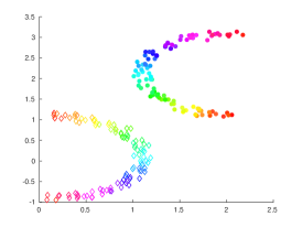
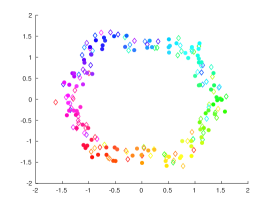
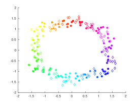
(a)                              (b)                              (c)

Figure 1: This figure shows the realignment results of CCA; (a) we consider 100 examples sampled from an “arc”, each sample is endowed with an RGB feature vector. We duplicate this dataset using a 2D rotation (with an angle of $180^{0}$) and we add a random perturbation field both to the color features and 2D coordinates. (b) realignment results obtained using standard CCA; note that original data are not aligned, so in order to apply standard CCA, each sample in the first arc-set is paired with its nearest (color descriptor) neighbor in the second arc-set. (c) realignment results obtained using our AA CCA approach; again data are not paired, so we consider a fully dense matrix D that measures the cross-similarity (using an RBF kernel) between the colors of the first and the second arc-sets. In these toy experiments, $\beta$ (weight of context regularizer) is set to $0.01$ and we use an isotropic neighborhood system in order to fill the context matrices $\{{\bf W}^{c}_{u}\}_{c=1}^{C}$, $\{{\bf W}^{c}_{v}\}_{c=1}^{C}$ (with $C=1$) and a given entry ${\bf W}^{c}_{u,i,k}$ is set to 1 iff $\mathbf{u}_{k}$ is among the 10 spatial neighbors of $\mathbf{u}_{i}$. Similarly, we set the entries of $\{{\bf W}^{c}_{v}\}_{c}^{C}$. For a better visualization of these results, better to view/zoom the PDF of this paper.

3.2 Satellite Image Change Detection

We also evaluate and compare the performance of our proposed AA CCA method on the challenging task of satellite image change detection (see for instance [51, 52, 53, 8, 54, 55, 56, 57, 58]). The goal is to find instances of relevant changes into a given scene acquired at instance $t_{1}$ with respect to the same scene taken at instant $t_{0}<t_{1}$; these acquisitions (at instants $t_{0}$, $t_{1}$) are referred to as reference and test images respectively. This task is known to be very challenging due to the difficulty to characterize relevant changes (appearance or disappearance of objects) from irrelevant ones such as the presence of cars, clouds, as well as registration errors. This task is also practically important; indeed, in the particular important scenario of damage assessment after natural hazards (such as tornadoes, earth quakes, etc.), it is crucial to achieve automatic change detection accurately in order to organize and prioritize rescue operations.

3.2.1 JOPLIN-TORNADOES11 Dataset

This dataset includes 680928 non overlapping image patches (of 30 $\times$ 30 pixels in RGB) taken from six pairs of (reference and test) GeoEye-1 satellite images (of 9850 $\times$ 10400 pixels each). This dataset is randomly split into two subsets: labeled used for training (denoted ${\cal L}_{r}\subset{\cal I}_{r}$, ${\cal L}_{t}\subset{\cal I}_{t}$) and unlabeled used for testing (denoted ${\cal U}_{r}={\cal I}_{r}\backslash{\cal L}_{r}$ and ${\cal U}_{t}={\cal I}_{t}\backslash{\cal L}_{t}$) with $|{\cal L}_{r}|=|{\cal L}_{t}|=3000$ and $|{\cal U}_{r}|=|{\cal U}_{t}|=680928-3000$. All patches in ${\cal I}_{r}$ (or in ${\cal I}_{t}$), stitched together, cover a very large area – of about 20 $\times$ 20 km² – around Joplin (Missouri) and show many changes after tornadoes that happened in may 2011 (building destruction, etc.) and no-changes (including irrelevant ones such as car appearance/disappearance, etc.). Each patch in ${\cal I}_{r}$, ${\cal I}_{t}$ is rescaled and encoded with 4096 coefficients corresponding to the output of an inner layer of the pretrained VGG-net [59]. A given test patch is declared as a “change” or “no-change” depending on the score of SVMs trained on top of the learned CCA latent representations.
In order to evaluate the performances of change detection, we report the equal error rate (EER). The latter is a balanced generalization error that equally weights errors in “change” and “no-change” classes. Smaller EER implies better performance.

3.2.2 Data Pairing and Context Regularization

In order to study the impact of AA CCA on the performances of change detection – both with residual and relatively stronger misalignments – we consider the following settings for comparison (see also table. I).

• Standard CCA: patches are strictly paired by assigning each patch, in the reference image, to a unique patch in the test image (in the same location), so it assumes that satellite images are correctly registered. CCA learning is supervised (only labeled patches are used for training) and no-context regularization is used (i.e, $\beta=0$). In order to implement this setting, we consider D as a diagonal matrix with $\textbf{D}_{ii}=\pm 1$ depending on whether $\mathbf{v}_{i}\in{\cal L}_{t}$ is labeled as “no-change” (or “change”) in the ground-truth, and $\textbf{D}_{ii}=0$ otherwise.

• Sup+CA CCA: this is similar to “standard CCA”with the only difference being $\beta$ which is set to its “optimal” value ($0.01$) on the validation set (see Fig. 2).

• SemiSup CCA: this setting is similar to “standard CCA” with the only difference being the unlabeled patches which are now added when learning the CCA transformations, and $\textbf{D}_{ii}$ (on the unlabeled patches) is set to $2\kappa(\mathbf{v}_{i},\mathbf{u}_{i})-1$ (score between $-1$ and $+1$); here $\kappa(.,.)\in[0,1]$ is the RBF similarity whose scale is set to the 0.1 quantile of pairwise distances in ${\cal L}_{t}\times{\cal L}_{r}$.

• SemiSup+CA CCA: this setting is similar to “SemiSup CCA” but context regularization is used (with again $\beta$ set to $0.01$).

• Res CCA: this is similar to “standard CCA”, but strict data pairing is relaxed, i.e., each patch in the reference image is assigned to multiple patches in the test image; hence, D is no longer diagonal, and set as $\textbf{D}_{ij}=\kappa(\mathbf{v}_{i},\mathbf{u}_{j})\in[0,1]$ iff $(\mathbf{v}_{i},\mathbf{u}_{j})\in{\cal L}_{t}\times{\cal L}_{r}$ is labeled as “no-change” in the ground-truth, $\textbf{D}_{ij}=\kappa(\mathbf{v}_{i},\mathbf{u}_{j})-1\in[-1,0]$ iff $(\mathbf{v}_{i},\mathbf{u}_{j})\in{\cal L}_{t}\times{\cal L}_{r}$ is labeled as “change” and $\textbf{D}_{ij}=0$ otherwise.

• Res+Sup+CA CCA: this is similar to “Res CCA”with the only difference being $\beta$ which is again set to $0.01$.

• Res+SemiSup CCA: this setting is similar to “Res CCA” with the only difference being the unlabeled patches which are now added when learning the CCA transformations; on these unlabeled patches $\textbf{D}_{ij}=2\kappa(\mathbf{v}_{i},\mathbf{u}_{j})-1$.

• Res+SemiSup+CA CCA: this setting is similar to “Res+SemiSup CCA” but context regularization is used (i.e., $\beta=0.01$).

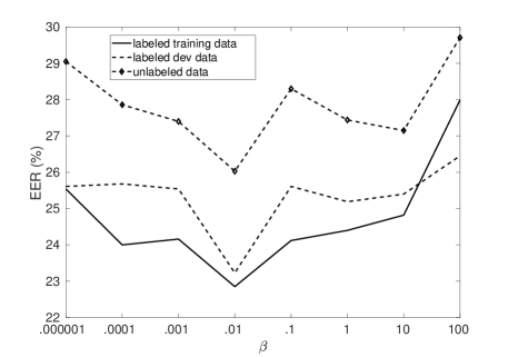
Figure 2: This figure shows the evolution of change detection performances w.r.t $\beta$ on labeled training/dev data as well as the unlabeled data. These results correspond to the baseline Sup+CA CCA (under the regime of strong misalignments); we observe from these curves that $\beta=0.01$ is the best setting which is kept in all our experiments.

Context setting: in order to build the adjacency matrices of the context (see section 2.3), we define for each patch $\mathbf{u}_{i}\in{\cal I}_{r}$ (in the reference image) an anisotropic (typed) neighborhood system $\{{\cal N}_{c}(i)\}_{c=1}^{C}$ (with $C=8$) which corresponds to the eight spatial neighbors of $\mathbf{u}_{i}$ in a regular grid [60, 61, 62]; for instance when $c=1$, ${\cal N}_{1}(i)$ corresponds to the top-left neighbor of $\mathbf{u}_{i}$. Using $\{{\cal N}_{c}(.)\}_{c=1}^{8}$, we build for each $c$ an intrinsic adjacency matrix ${\bf W}^{c}_{u}$ whose $(i,k)^{\textrm{th}}$ entry is set as ${\bf W}^{c}_{u,i,k}\propto\mathds{1}_{\{k\in{\cal N}_{c}(i)\}}$; here $\mathds{1}_{\{\}}$ is the indicator function equal to $1$ iff i) the patch $\mathbf{u}_{k}$ is neighbor to $\mathbf{u}_{i}$ and ii) its relative position is typed as $c$ ($c=1$ for top-left, $c=2$ for left, etc. following an anticlockwise rotation), and $0$ otherwise. Similarly, we define the matrices $\{{\bf W}^{c}_{v}\}_{c}$ for data $\{\mathbf{v}_{j}\}_{j}\in{\cal I}_{t}$.

Pairing	CCA Learning	Context Regularization	Designation
strict	supervised	no	Standard CCA
strict	supervised	yes	Sup+CA CCA
strict	semi-sup	no	SemiSup CCA
strict	semi-sup	yes	SemiSup+CA CCA
relaxed	supervised	no	Res CCA
relaxed	supervised	yes	Res+Sup+CA CCA
relaxed	semi-sup	no	Res+SemiSup CCA
relaxed	semi-sup	yes	Res+SemiSup+CA CCA

TABLE I: This table shows different configurations of CCA resulting from different instances of our model. In this table, “Sup” stands for supervised, “SemiSup” for semi-supervised, “CA” for context aware and “Res” for resilient.

3.2.3 Impact of AA CCA and Comparison

Table. II shows a comparison of different versions of AA CCA against other CCA variants under the regime of small residual alignment errors. In this regime, reference and test images are first registered using RANSAC [63]; an exhaustive visual inspection of the overlapping (reference and test) images (after RANSAC registration) shows sharp boundaries in most of the areas covered by these images, but some areas still include residual misalignments due to the presence of changes, occlusions (clouds, etc.) as well as parallax. Note that, in spite of the relative success of RANSAC in registering these images, our AA CCA versions (rows #5–8) provide better performances (see table. II) compared to the other CCAs (rows #1–4); this clearly corroborates the fact that residual alignment errors remain after RANSAC (re)alignment (as also observed during visual inspection of RANSAC registration). Put differently, our AA CCA method is not an opponent to RANSAC but complementary.

#	Configurations	Labeled(train)	Labeled(dev)	Unlabeled
1	Standard CCA	14.91	15.18	12.81
2	Sup+CA CCA	12.95	14.90	11.44
3	SemiSup CCA	11.26	12.80	11.18
4	SemiSup+CA CCA	12.57	11.82	09.96
5	Res CCA	05.81	04.97	05.38
6	Res+Sup+CA CCA	06.35	05.53	05.55
7	Res+SemiSup CCA	08.60	08.74	08.33
8	Res+SemiSup+CA CCA	08.77	08.60	06.94

TABLE II: This table shows change detection EER (in %) on labeled (training and validation) and unlabeled sets under the residual error regime. When context regularization (referred to as CA in this table) is used, $\beta$ is set to $10^{\small-2}$.

These results also show that when reference and test images are globally well aligned (with some residual errors; see table. II), the gain in performance is dominated by the positive impact of alignment resilience; indeed, the impact of the unlabeled data is not always consistent (#5,6 vs. #7,8 resp.) in spite of being positive (in #1,2 vs. #3,4 resp.) while the impact of context regularization is globally positive (#1,3,5,7 vs. #2,4,6,8 resp.). This clearly shows that, under the regime of small residual errors, the use of labeled data is already enough in order to enhance the performance of change detection; the gain comes essentially from alignment resilience with a marginal (but clear) positive impact of context regularization.
In order to study the impact of AA CCA w.r.t stronger alignment errors (i.e. w.r.t a more challenging setting), we apply a relatively strong motion field to all the pixels in the reference image; precisely, each pixel is shifted along a direction whose x–y coordinates are randomly set to values between 15 and 30 pixels. These shifts are sufficient in order to make the quality of alignments used for CCA very weak so the different versions of CCA, mentioned earlier, become more sensitive to alignment errors (EERs increase by more than 100% in table. III compared to EERs with residual alignment errors in table. II). With this setting, AA CCA is clearly more resilient and shows a substantial relative gain compared to the other CCA versions.

#	Configurations	Labeled(train)	Labeled(dev)	Unlabeled
1	Standard CCA	25.63	25.61	28.44
2	Sup+CA CCA	22.85	23.23	26.03
3	SemiSup CCA	22.31	23.58	24.99
4	SemiSup+CA CCA	25.74	25.40	25.47
5	Res CCA	16.42	14.34	19.67
6	Res+Sup+CA CCA	16.55	16.80	19.90
7	Res+SemiSup CCA	19.01	19.24	19.55
8	Res+SemiSup+CA CCA	23.71	21.55	26.76

TABLE III: This table shows change detection EER (in %) on labeled (training and validation) and unlabeled sets under the strong error regime. When context regularization (referred to as CA in this table) is used, $\beta$ is set to $10^{-2}$.

3.3 Discussion

Invariance: resulting from its misalignment resilience, it is easy to see that our AA CCA is de facto robust to local deformations as these deformations are strictly equivalent to local misalignments. It is also easy to see that our AA CCA may achieve invariance to similarity transformations; indeed, the matrices used to define the spatial context are translation invariant, and can also be made rotation and scale invariant by measuring a “characteristic” scale and orientation of patches in a given satellite image. For that purpose, dense SIFT can be used to recover (or at least approximate) the field of orientations and scales, and hence adapt the spatial support (extent and orientation) of context using the characteristic scale, in order to make context invariant to similarity transformations.

Computational Complexity: provided that VGG-features are extracted (offline) on all the patches of the reference/test images, and provided that the adjacency matrices of context are precomputed, and since the adjacency matrices $\{{\bf W}^{c}_{u}\}_{c}$, $\{{\bf W}^{c}_{v}\}_{c}$ are very sparse, the computational complexity of evaluating Eq. (6) and solving the generalized eigenproblem in  Eq. (5) both reduce to $O(\min(d_{u}^{2}d_{v},d_{v}^{2}d_{u}))$, here $d_{u}$, $d_{v}$ are again the dimensions of data in U, V respectively; hence, this complexity is very equivalent to standard CCA which also requires solving a generalized eigenproblem. Therefore, the gain in the accuracy of our AA CCA is obtained without any overhead in the computational complexity that remains dependent on dimensionality of data (which is, in practice, smaller compared to the cardinality of our datasets).

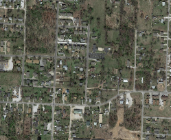
Ref image

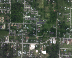
Test image + GT mask

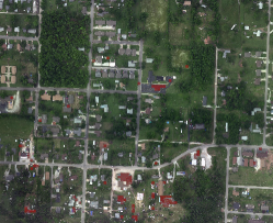
Standard CCA

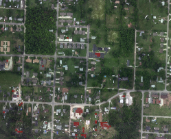
Sup CCA+CA

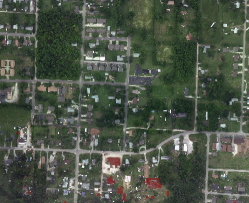
Res CCA

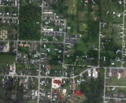
Res CCA+CA

Figure 3: These examples show the evolution of detections (in red) for four different settings of CCA; as we go from top-right to bottom-right, change detection results get better. CCA acronyms shown below pictures are already defined in Table.1.

4 Conclusion

We introduced in this paper a new canonical correlation analysis method that learns projection matrices which map data from input spaces to a latent common space where unaligned data become strongly or weakly correlated depending on their cross-view similarity and their context. This is achieved by optimizing a criterion that mixes two terms: the first one aims at maximizing the correlations between data which are likely to be paired while the second term acts as a regularizer and makes correlations spatially smooth and provides us with robust context-aware latent representations. Our method considers both labeled and unlabeled data when learning the CCA projections while being resilient to alignment errors. Extensive experiments show the substantial gain of our CCA method under the regimes of residual and strong alignment errors.

As a future work, our CCA method can be extended to many other tasks where alignments are error-prone and when context can be exploited in order to recover from these alignment errors. These tasks include “text-to-text” alignment in multilingual machine translation, as well as “image-to-image” matching in multi-view object tracking.

Appendix A Appendix (proof of Proposition 2)

We will prove that $\Psi$ is $L$-Lipschitzian,
with $L=\frac{\beta}{\gamma_{\min}}\big{(}\sum_{c}\big{\|}{\bf E}_{c}\ {\bf 1}_{\tiny vu}\ {\bf F}_{c}^{\prime}\big{\|}_{1}+\sum_{c}\big{\|}{\bf G}_{c}\ {\bf 1}_{\tiny vu}\ {\bf H}_{c}^{\prime}\big{\|}_{1}\big{)}$. For ease of writing, we omit in this proof the subscripts $t$, $r$ in ${\bf K}_{tr}$ (unless explicitly required and mentioned).
Given two matrices ${\bf K}^{(2)}$, ${\bf K}^{(1)}$, we have $\big{\|}{\bf K}^{(2)}-{\bf K}^{(1)}\big{\|}_{1}=(*)$ with

$$\begin{array}[]{ll}(*)&=\displaystyle\beta\bigg{\|}\sum_{c}\textbf{V}{\bf W}^{c}_{v}\textbf{V}^{\prime}({\textbf{P}_{t}}^{(1)}{\textbf{P}^{\prime}_{r}}^{(1)}-{\textbf{P}_{t}}^{(0)}{\textbf{P}^{\prime}_{r}}^{(0)})\textbf{U}{\bf W}^{c^{\prime}}_{u}\textbf{U}^{\prime}\\ &\ \ \ \ +\displaystyle\ \sum_{c}\textbf{V}{\bf W}^{c^{\prime}}_{v}\textbf{V}^{\prime}({\textbf{P}_{t}}^{(1)}{\textbf{P}^{\prime}_{r}}^{(1)}-{\textbf{P}_{t}}^{(0)}{\textbf{P}^{\prime}_{r}}^{(0)})\textbf{U}{\bf W}^{c}_{u}\textbf{U}^{\prime}\bigg{\|}_{1}.\end{array}$$ (12)

Using Eq. (5), one may write

$${\textbf{P}_{t}}{\textbf{P}^{\prime}_{r}}=\frac{1}{\gamma}\textbf{C}_{tt}^{-1}{\bf K}_{tr}\textbf{C}_{rr}^{-1},$$ (13)

which also results from the fact that ${\bf K}_{rt}\textbf{C}_{tt}^{-1}{\bf K}_{tr}$ is Hermitian and $\textbf{C}_{rr}$ is positive semi-definite. By adding the superscript $\tau$ in ${\textbf{P}_{t}}$, ${\textbf{P}_{r}}$, $\gamma$, ${\bf K}_{tr}$ (with $\tau=0,1$), omitting again the subscripts $t$, $r$ in ${\bf K}_{tr}$ and then plugging (13) into (12) we obtain

$$\small\begin{array}[]{lll}(*)&=&\displaystyle\beta\bigg{\|}\sum_{c}{\bf E}_{c}\ (\frac{1}{\gamma^{(1)}}{\bf K}^{(1)}-\frac{1}{\gamma^{(0)}}{\bf K}^{(0)})\ {\bf F}^{\prime}_{c}+\displaystyle\ \sum_{c}{\bf G}_{c}\ (\frac{1}{\gamma^{(1)}}{\bf K}^{(1)}-\frac{1}{\gamma^{(0)}}{\bf K}^{(0)})\ {\bf H}_{c}^{\prime}\bigg{\|}_{1}\\ &\leq&\displaystyle\frac{\beta}{\gamma_{\min}}\bigg{\|}\sum_{c}{\bf E}_{c}\ ({\bf K}^{(1)}-{\bf K}^{(0)})\ {\bf F}_{c}^{\prime}\bigg{\|}_{1}+\ \displaystyle\frac{\beta}{\gamma_{\min}}\bigg{\|}\sum_{c}{\bf G}_{c}\ ({\bf K}^{(1)}-{\bf K}^{(0)})\ {\bf H}_{c}^{\prime}\bigg{\|}_{1},\end{array}$$ (14)

here $\gamma_{\min}$ is the lower bound of the eigenvalues of (5) which can be derived (see for instance [64]). Considering ${\bf K}_{k,\ell}$ as the $(k,\ell)^{\rm{th}}$ entry of ${\bf K}$, we have

$$\small\begin{array}[]{lll}(*)&\leq&\ \ \frac{\beta}{\gamma_{\min}}\displaystyle\sum_{i,j}\bigg{|}\displaystyle\sum_{k,\ell}({\bf K}^{(1)}_{k,\ell}-{\bf K}^{(0)}_{k,\ell})\sum_{c}{\bf E}_{c,i,k}\ {\bf F}_{c,j,\ell}\bigg{|}\\ &&\ \ \ +\frac{\beta}{\gamma_{\min}}\displaystyle\sum_{i,j}\bigg{|}\displaystyle\sum_{k,\ell}({\bf K}^{(1)}_{k,\ell}-{\bf K}^{(0)}_{k,\ell})\sum_{c}{\bf G}_{c,i,k}\ {\bf H}_{c,j,\ell}\bigg{|}\\ &&\\ &{\bf\leq}&\ \ \frac{\beta}{\gamma_{\min}}\displaystyle\sum_{i,j}\displaystyle\sum_{k,\ell}\big{|}{\bf K}^{(1)}_{k,\ell}-{\bf K}^{(0)}_{k,\ell}\big{|}\sum_{c}\big{|}{\bf E}_{c,i,k}\ {\bf F}_{c,j,\ell}\big{|}\\ &&\ \ \ +\frac{\beta}{\gamma_{\min}}\displaystyle\sum_{i,j}\displaystyle\sum_{k,\ell}\big{|}{\bf K}^{(1)}_{k,\ell}-{\bf K}^{(0)}_{k,\ell}\big{|}\sum_{c}\big{|}{\bf G}_{c,i,k}\ {\bf H}_{c,j,\ell}\big{|}\\ &&\\ &\leq&\ \ \frac{\beta}{\gamma_{\min}}\displaystyle\sum_{k,\ell}\big{|}{\bf K}^{(1)}_{k,\ell}-{\bf K}^{(0)}_{k,\ell}\big{|}\\ &&\ \times\bigg{(}\displaystyle\sum_{i,j}\sum_{k,\ell,c}\big{|}{\bf E}_{c,i,k}\ {\bf F}_{c,j,\ell}\big{|}+\displaystyle\sum_{i,j}\sum_{k,\ell,c}\big{|}{\bf G}_{c,i,k}\ {\bf H}_{c,j,\ell}\big{|}\bigg{)}\\ &&(\textrm{as}\ \sum_{i}|a_{i}|.|b_{i}|\leq\sum_{i,j}|a_{i}|.|b_{j}|,\ \forall\ \{a_{i}\}_{i},\{b_{j}\}_{i}\subset\mathbb{R})\\ &&\\ &=&L\ \big{\|}{\bf K}^{(1)}-{\bf K}^{(0)}\big{\|}_{1},\end{array}$$

$$\small\textrm{with}\ \ \ L=\frac{\beta}{\gamma_{\min}}\big{(}\sum_{c}\big{\|}{\bf E}_{c}\ {\bf 1}_{\tiny vu}\ {\bf F}_{c}^{\prime}\big{\|}_{1}+\sum_{c}\big{\|}{\bf G}_{c}\ {\bf 1}_{\tiny vu}\ {\bf H}_{c}^{\prime}\big{\|}_{1}\big{)}\Box$$

References

- [1] A. Krizhevsky, I. Sutskever, and G. E. Hinton, “Imagenet classification with deep convolutional neural networks,” in Advances in neural information processing systems, 2012, pp. 1097–1105.
- [2] H. Sahbi, “Cnrs-telecom paristech at imageclef 2013 scalable concept image annotation task: Winning annotations with context dependent svms.” in CLEF (Working Notes), 2013.
- [3] O. Russakovsky, J. Deng, H. Su, J. Krause, S. Satheesh, S. Ma, Z. Huang, A. Karpathy, A. Khosla, M. Bernstein et al., “Imagenet large scale visual recognition challenge,” International Journal of Computer Vision, vol. 115, no. 3, pp. 211–252, 2015.
- [4] N. Boujemaa, F. Fleuret, V. Gouet, and H. Sahbi, “Visual content extraction for automatic semantic annotation of video news,” in the proceedings of the SPIE Conference, San Jose, CA, vol. 6, 2004.
- [5] L. Wang and H. Sahbi, “Directed acyclic graph kernels for action recognition,” in Proceedings of the IEEE International Conference on Computer Vision, 2013, pp. 3168–3175.
- [6] S. Tollari, P. Mulhem, M. Ferecatu, H. Glotin, M. Detyniecki, P. Gallinari, H. Sahbi, and Z.-Q. Zhao, “A comparative study of diversity methods for hybrid text and image retrieval approaches,” in Workshop of the Cross-Language Evaluation Forum for European Languages. Springer, 2008, pp. 585–592.
- [7] M. Ferecatu and H. Sahbi, “Telecomparistech at imageclefphoto 2008: Bi-modal text and image retrieval with diversity enhancement.” in CLEF (Working Notes), 2008.
- [8] M. Hussain, D. Chen, A. Cheng, H. Wei, and D. Stanley, “Change detection from remotely sensed images: From pixel-based to object-based approaches,” ISPRS Journal of Photogrammetry and Remote Sensing, vol. 80, pp. 91–106, 2013.
- [9] N. Bourdis, D. Marraud, and H. Sahbi, “Spatio-temporal interaction for aerial video change detection,” in Geoscience and Remote Sensing Symposium (IGARSS), 2012 IEEE International. IEEE, 2012, pp. 2253–2256.
- [10] T. Postadjian, A. Le Bris, H. Sahbi, and C. Mallet, “Investigating the potential of deep neural networks for large-scale classification of very high resolution satellite images,” ISPRS Annals of Photogrammetry, Remote Sensing and Spatial Information Sciences, pp. 183–190, 2017.
- [11] H. Sahbi and N. Boujemaa, “Coarse-to-fine support vector classifiers for face detection,” in the International Conference on Pattern Recognition. IEEE, 2002, p. 30359.
- [12] X. Li and H. Sahbi, “Superpixel-based object class segmentation using conditional random fields,” in Acoustics, Speech and Signal Processing (ICASSP), 2011 IEEE International Conference on. IEEE, 2011, pp. 1101–1104.
- [13] K. He, X. Zhang, S. Ren, and J. Sun, “Deep residual learning for image recognition,” in Proceedings of the IEEE conference on computer vision and pattern recognition, 2016, pp. 770–778.
- [14] I. Goodfellow, Y. Bengio, and A. Courville, “Deep learning. book in preparation for mit press,” URL¡ http://www. deeplearningbook. org, 2016.
- [15] M. Jiu and H. Sahbi, “Nonlinear deep kernel learning for image annotation,” IEEE Transactions on Image Processing, vol. 26, no. 4, pp. 1820–1832, 2017.
- [16] D. Erhan, Y. Bengio, A. Courville, P.-A. Manzagol, P. Vincent, and S. Bengio, “Why does unsupervised pre-training help deep learning?” Journal of Machine Learning Research, vol. 11, no. Feb, pp. 625–660, 2010.
- [17] J. Yosinski, J. Clune, Y. Bengio, and H. Lipson, “How transferable are features in deep neural networks?” in Advances in neural information processing systems, 2014, pp. 3320–3328.
- [18] C. Doersch and A. Zisserman, “Multi-task self-supervised visual learning,” arXiv preprint arXiv:1708.07860, 2017.
- [19] S. R. Richter, V. Vineet, S. Roth, and V. Koltun, “Playing for data: Ground truth from computer games,” in European Conference on Computer Vision. Springer, 2016, pp. 102–118.
- [20] H. Hotelling, “Relations between two sets of variates,” Biometrika, vol. 28, no. 3/4, pp. 321–377, 1936.
- [21] T. W. Anderson, An introduction to multivariate statistical analysis. Wiley New York, 1958, vol. 2.
- [22] D. R. Hardoon, S. Szedmak, and J. Shawe-Taylor, “Canonical correlation analysis: An overview with application to learning methods,” Neural computation, vol. 16, no. 12, pp. 2639–2664, 2004.
- [23] H. Sahbi, “Interactive satellite image change detection with context-aware canonical correlation analysis,” IEEE Geoscience and Remote Sensing Letters, vol. 14, no. 5, pp. 607–611, 2017.
- [24] T. Melzer, M. Reiter, and H. Bischof, “Appearance models based on kernel canonical correlation analysis,” Pattern recognition, vol. 36, no. 9, pp. 1961–1971, 2003.
- [25] D. R. Hardoon and J. Shawe-Taylor, “Sparse canonical correlation analysis,” Machine Learning, vol. 83, no. 3, pp. 331–353, 2011.
- [26] D. M. Witten and R. J. Tibshirani, “Extensions of sparse canonical correlation analysis with applications to genomic data,” Statistical applications in genetics and molecular biology, vol. 8, no. 1, pp. 1–27, 2009.
- [27] Z. Zhang, M. Zhao, and T. W. Chow, “Binary-and multi-class group sparse canonical correlation analysis for feature extraction and classification,” IEEE Transactions on Knowledge and Data Engineering, vol. 25, no. 10, pp. 2192–2205, 2013.
- [28] J. Vía, I. Santamaría, and J. Pérez, “A learning algorithm for adaptive canonical correlation analysis of several data sets,” Neural Networks, vol. 20, no. 1, pp. 139–152, 2007.
- [29] T. Sun and S. Chen, “Locality preserving cca with applications to data visualization and pose estimation,” Image and Vision Computing, vol. 25, no. 5, pp. 531–543, 2007.
- [30] D. Zhai, Y. Zhang, D.-Y. Yeung, H. Chang, X. Chen, and W. Gao, “Instance-specific canonical correlation analysis,” Neurocomputing, vol. 155, pp. 205–218, 2015.
- [31] F. Yger, M. Berar, G. Gasso, and A. Rakotomamonjy, “Adaptive canonical correlation analysis based on matrix manifolds,” arXiv preprint arXiv:1206.6453, 2012.
- [32] F. De la Torre, “A unification of component analysis methods,” Handbook of pattern recognition and computer vision, pp. 3–22, 2009.
- [33] J. Sun and S. Keates, “Canonical correlation analysis on data with censoring and error information,” IEEE transactions on neural networks and learning systems, vol. 24, no. 12, pp. 1909–1919, 2013.
- [34] L. Sun, S. Ji, and J. Ye, “Canonical correlation analysis for multilabel classification: A least-squares formulation, extensions, and analysis,” IEEE Transactions on Pattern Analysis and Machine Intelligence, vol. 33, no. 1, pp. 194–200, 2011.
- [35] M. Haghighat and M. Abdel-Mottaleb, “Low resolution face recognition in surveillance systems using discriminant correlation analysis,” in Automatic Face & Gesture Recognition (FG 2017), 2017 12th IEEE International Conference on. IEEE, 2017, pp. 912–917.
- [36] M. Ferecatu and H. Sahbi, “Multi-view object matching and tracking using canonical correlation analysis,” in Image Processing (ICIP), 2009 16th IEEE International Conference on. IEEE, 2009, pp. 2109–2112.
- [37] C. C. Loy, T. Xiang, and S. Gong, “Multi-camera activity correlation analysis,” in Computer Vision and Pattern Recognition, 2009. CVPR 2009. IEEE Conference on. IEEE, 2009, pp. 1988–1995.
- [38] F. Zhou and F. Torre, “Canonical time warping for alignment of human behavior,” in Advances in neural information processing systems, 2009, pp. 2286–2294.
- [39] F. Zhou and F. De la Torre, “Generalized canonical time warping,” IEEE transactions on pattern analysis and machine intelligence, vol. 38, no. 2, pp. 279–294, 2016.
- [40] T.-K. Kim and R. Cipolla, “Canonical correlation analysis of video volume tensors for action categorization and detection,” IEEE Transactions on Pattern Analysis and Machine Intelligence, vol. 31, no. 8, pp. 1415–1428, 2009.
- [41] B. Fischer, V. Roth, and J. M. Buhmann, “Time-series alignment by non-negative multiple generalized canonical correlation analysis,” BMC bioinformatics, vol. 8, no. 10, p. S4, 2007.
- [42] G. Trigeorgis, M. Nicolaou, S. Zafeiriou, and B. Schuller, “Deep canonical time warping for simultaneous alignment and representation learning of sequences,” IEEE Transactions on Pattern Analysis and Machine Intelligence, 2017.
- [43] J. Ham, D. D. Lee, and L. K. Saul, “Semisupervised alignment of manifolds.” in AISTATS, 2005, pp. 120–127.
- [44] S. Lafon, Y. Keller, and R. R. Coifman, “Data fusion and multicue data matching by diffusion maps,” IEEE Transactions on pattern analysis and machine intelligence, vol. 28, no. 11, pp. 1784–1797, 2006.
- [45] C. Wang and S. Mahadevan, “Manifold alignment using procrustes analysis,” in Proceedings of the 25th international conference on Machine learning. ACM, 2008, pp. 1120–1127.
- [46] B. Luo and E. R. Hancock, “Iterative procrustes alignment with the em algorithm,” Image and Vision Computing, vol. 20, no. 5, pp. 377–396, 2002.
- [47] K. D. Feuz and D. J. Cook, “Collegial activity learning between heterogeneous sensors,” Knowledge and Information Systems, pp. 1–28, 2017.
- [48] H. Sahbi, J.-Y. Audibert, J. Rabarisoa, and R. Keriven, “Context-dependent kernel design for object matching and recognition,” in CVPR, 2008, pp. 1–8.
- [49] H. Sahbi and X. Li, “Context-based support vector machines for interconnected image annotation,” in Asian Conference on Computer Vision. Springer, 2010, pp. 214–227.
- [50] D. Chetverikov, D. Stepanov, and P. Krsek, “Robust euclidean alignment of 3d point sets: the trimmed iterative closest point algorithm,” Image Vision Comput., vol. 23, no. 3, pp. 299–309, 2005.
- [51] H. Sahbi, “Discriminant canonical correlation analysis for interactive satellite image change detection.” in IGARSS, 2015, pp. 2789–2792.
- [52] R. J. Radke, S. Andra, O. Al-Kofahi, and B. Roysam, “Image change detection algorithms: a systematic survey,” IEEE Trans. Image Processing, vol. 14, no. 3, pp. 294–307, 2005.
- [53] N. Bourdis, M. Denis, and H. Sahbi, “Constrained optical flow for aerial image change detection,” in 2011 IEEE International Geoscience and Remote Sensing Symposium (IGARSS), 2011, pp. 4176–4179.
- [54] H. Sahbi, “Coarse-to-fine deep kernel networks,” in IEEE International Conference on Computer Vision Workshops, ICCV Workshops, 2017, pp. 1131–1139.
- [55] N. Bourdis, M. Denis, and H. Sahbi, “Camera pose estimation using visual servoing for aerial video change detection,” in 2012 IEEE International Geoscience and Remote Sensing Symposium (IGARSS), 2012, pp. 3459–3462.
- [56] T. Çelik, “Image change detection using gaussian mixture model and genetic algorithm,” J. Visual Communication and Image Representation, vol. 21, no. 8, pp. 965–974, 2010.
- [57] L. I. Kuncheva and W. J. Faithfull, “PCA feature extraction for change detection in multidimensional unlabelled streaming data,” in Proceedings of the 21st International Conference on Pattern Recognition, ICPR 2012, Tsukuba, Japan, November 11-15, 2012, 2012, pp. 1140–1143.
- [58] H. Sahbi, “Relevance feedback for satellite image change detection,” in Acoustics, Speech and Signal Processing (ICASSP), 2013 IEEE International Conference on. IEEE, 2013, pp. 1503–1507.
- [59] K. Simonyan and A. Zisserman, “Very deep convolutional networks for large-scale image recognition,” CoRR, vol. abs/1409.1556, 2014.
- [60] S. Thiemert, H. Sahbi, and M. Steinebach, “Applying interest operators in semi-fragile video watermarking,” in Security, Steganography, and Watermarking of Multimedia Contents VII, vol. 5681. International Society for Optics and Photonics, 2005, pp. 353–363.
- [61] J. Jeon and R. Manmatha, “Using maximum entropy for automatic image annotation,” in Image and Video Retrieval: Third International Conference, CIVR 2004, Dublin, Ireland, July 21-23, 2004. Proceedings, 2004, pp. 24–32.
- [62] S. Thiemert, H. Sahbi, and M. Steinebach, “Using entropy for image and video authentication watermarks,” in Security, Steganography, and Watermarking of Multimedia Contents VIII, vol. 6072. International Society for Optics and Photonics, 2006, p. 607218.
- [63] T. Kim and Y.-J. Im, “Automatic satellite image registration by combination of matching and random sample consensus,” IEEE transactions on geoscience and remote sensing, vol. 41, no. 5, pp. 1111–1117, 2003.
- [64] L.-Z. Lu and C. E. M. Pearce, “Some new bounds for singular values and eigenvalues of matrix products,” Annals of Operations Research, vol. 98, no. 1, pp. 141–148, 2000.