The discovery of WASP-134b, WASP-134c, WASP-137b, WASP-143b and WASP-146b: three hot Jupiters and a pair of warm Jupiters orbiting Solar-type stars

Abstract

We report the discovery by WASP of five planets orbiting moderately bright ($V$ = 11.0–12.9) Solar-type stars. WASP-137b, WASP-143b and WASP-146b are typical hot Jupiters in orbits of 3–4 d and with masses in the range 0.68–1.11 $M_{\rm Jup}$. WASP-134 is a metal-rich ([Fe/H] = +0.40 $\pm$ 0.07]) G4 star orbited by two warm Jupiters: WASP-134b ($M_{\rm P}$ = 1.41 $M_{\rm Jup}$; $P=10.1$ d; $e=0.15\pm 0.01$; $T_{\rm eql}$ = 950 K) and WASP-134c ($M_{\rm P}$ $\sin i$ = 0.70 $M_{\rm Jup}$; $P=70.0$ d; $e=0.17\pm 0.09$; $T_{\rm eql}$ = 500 K). From observations of the Rossiter-McLaughlin effect of WASP-134b, we find its orbit to be misaligned with the spin of its star ($\lambda=-44\pm 10^{\circ}$). WASP-134 is a rare example of a system with a short-period giant planet and a nearby giant companion. In-situ formation or disc migration seem more likely explanations for such systems than does high-eccentricity migration.

1 Introduction

As we near a tally of 200 planets discovered by our ground-based transit survey WASP (Pollacco et al., 2006), TESS is ushering in the era of space-based wide-field transit surveys (Ricker et al., 2014). TESS will provide an important test of the completeness of WASP, as well as of similar surveys such as KELT (Pepper et al., 2007), HATNet and HATSouth (Bakos, 2018).

Considering that during its nominal mission TESS will observe most of its target fields for only 27 days, it faces a challenge to discover planets with periods longer than half that duration. For some of those planets for which TESS observes only one or two transits, ephemerides may be recovered by combining the TESS data with the long baseline of the aforementioned surveys (Yao et al., 2018). Though each of those surveys is multi-site, even single-site observations would be effective in following up TESS’s single-transit detections (Cooke et al., 2018). Thus ground-based projects such as TRAPPIST (Gillon et al., 2011; Jehin et al., 2011), NGTS (Wheatley et al., 2018) and SPECULOOS (Delrez et al., 2018) stand to play an important role, as does ESA’s CHEOPS satellite (Broeg et al., 2013), which is scheduled for launch in late 2019.

Warm Jupiters (orbital period $P$ = 10–200 d) are more difficult to find than are hot Jupiters, due to their lower geometric transit probability, less frequent transits, and longer transit durations. Also, they may be inherently less common (e.g. Santerne et al. 2016). Considering only ‘Jupiters’ (planets with mass $M_{\rm P}$ $>$ 0.3 $M_{\rm Jup}$), the TEPCat database lists 416 hot Jupiters ($P<10$ d), but only 37 Jupiters in the range $P$ = 10–20 d (Southworth, 2011).

Longer-period planets are certainly worth the effort required to find them: to gain an understanding of the diversity of exoplanets, their various formation and evolution histories, bulk and atmospheric compositions, etc., we must populate a wide region of parameter space. Specifically, by measuring the orbital eccentricities and stellar obliquities of planets in the tail end of the hot-Jupiter period distribution, where tides are weak, it may be that we can explain hot Jupiter migration (e.g. Anderson et al. 2015a).

While it is common for a hot Jupiter to have a massive companion in a wide orbit (e.g. Howard et al. 2012; Neveu-VanMalle et al. 2016; Triaud et al. 2017), no hot Jupiters are known to have close companions (with the notable exception of WASP-47b; Hellier et al. 2012; Becker et al. 2015). Conversely, half of warm Jupiters are flanked by small companions, which Huang et al. (2016) interpreted as indicating that warm Jupiters formed in situ.

We report here the discovery by the WASP survey of five planets orbiting Sun-like stars. In three systems we detect a single hot Jupiter and in the fourth system we detect two warm Jupiters. We measure the orbital eccentricity of both warm Jupiters and the stellar obliquity of the inner planet.

2 Observations

From periodic dimmings seen in their SuperWASP-North and WASP-South lightcurves (Pollacco et al. 2006; top panel of Figs. 1, 2, 3 and 4), we identified each star as a candidate host of a transiting planet using the techniques described in Collier Cameron et al. (2006, 2007). We conducted photometric and spectroscopic follow-up observations using various facilities at the ESO La Silla observatory: the EulerCam imager and the CORALIE spectrograph, both mounted on the 1.2-m Swiss Euler telescope (Lendl et al., 2012; Queloz et al., 2000), the 0.6-m TRAPPIST-South imager (Gillon et al., 2011; Jehin et al., 2011), and the HARPS-S spectrograph on the 3.6-m ESO telescope (Pepe et al., 2002). We obtained additional data using the HARPS-N spectrograph on the 3.6-m Telescopio Nazionale Galileo at the Observatorio del Roque de los Muchachos (Cosentino et al., 2012). We provide a summary of our observations in Table 1.

Table 1: Summary of observations

Facility	Date	$N_{\rm obs}$	Notes
WASP-134
WASP	2008 Jun–2010 Oct	28 614	400–700 nm
TRAPPIST-South	2014 Sep 05	678	$I+z$
TRAPPIST-South	2014 Oct 26	284	$I+z$
Euler/EulerCam	2016 Sep 25	338	NGTS filter
Euler/CORALIE	2014 Jul–2018 Oct	33	orbit
ESO3.6/HARPS-S	2015 Jun–2015 Aug	10	orbit
ESO3.6/HARPS-S	2015 Aug 16	17	transit
TNG/HARPS-N	2018 Aug 16	47	transit
WASP-137
WASP	2008 Jul–2010 Dec	17 463	400–700 nm
TRAPPIST-South	2014 Nov 10	577	$I+z$
Euler/EulerCam	2014 Nov 14	303	Gunn $r$
TRAPPIST-South	2014 Dec 27	709	$I+z$
TRAPPIST-South	2015 Sep 03	982	$I+z$; MF
Euler/CORALIE	2014 Sep–2017 Jan	32	orbit
WASP-143
WASP	2009 Jan–2012 Apr	32 995	400–700 nm
TRAPPIST-South	2015 Jan 31	767	blue-blocking
Euler/EulerCam	2015 Feb 15	199	NGTS filter
Euler/EulerCam	2015 Mar 06	178	NGTS filter
TRAPPIST-South	2016 Feb 09	843	blue-blocking; MF
Euler/CORALIE	2014 Feb–2017 May	22	orbit
WASP-146
WASP	2008 Jun–2011 Nov	54 839	400–700 nm
Euler/EulerCam	2014 Nov 18	190	NGTS filter
TRAPPIST-South	2014 Nov 18	791	blue-blocking
Euler/EulerCam	2015 Jul 17	150	NGTS filter
TRAPPIST-South	2015 Jul 17	874	blue-blocking; MF
Euler/CORALIE	2014 Jul–2016 Oct	16	orbit

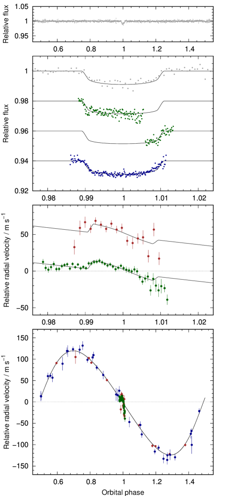
Figure 1: WASP-134b discovery data. Top panel: WASP lightcurve folded on the transit ephemeris and binned with a bin width of 10 min. Second panel: Transit lightcurves from WASP (grey), TRAPPIST-South (green) and EulerCam (blue), offset for clarity, binned with a bin width of 2 min (10 min for WASP), and plotted chronologically with the most recent lightcurve at the bottom. The best-fitting transit model is superimposed. Third panel: The RVs from HARPS-S (brown) and HARPS-N (green) showing the apparent anomaly during transit, along with the best-fitting Rossiter-McLaughlin (RM) effect model. Bottom panel: The RVs from CORALIE (blue), HARPS-S and HARPS-N, with the best-fitting eccentric orbital model. WASP-134 reached high airmass by the end of each photometric and spectroscopic transit sequence.

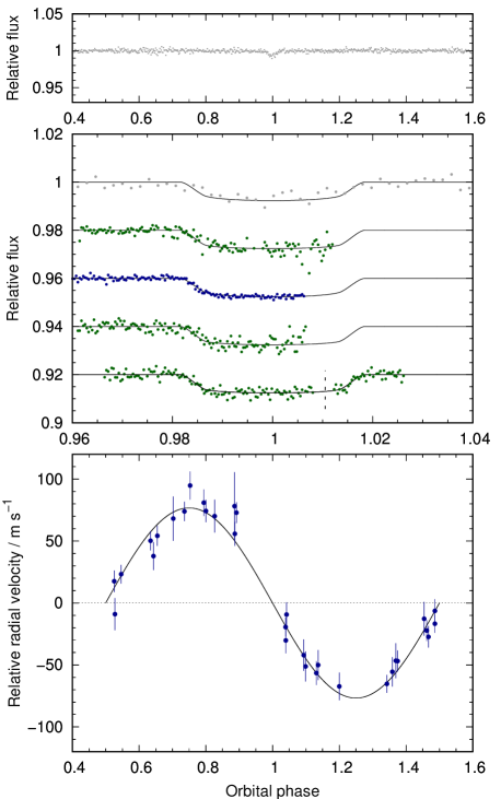
Figure 2: WASP-137b discovery data. As for Fig. 1. The meridian flip is indicated with a vertical dashed line.

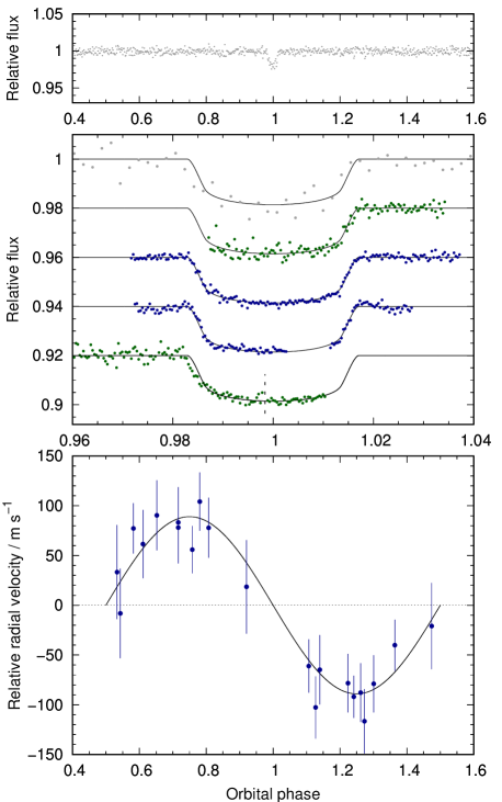
Figure 3: WASP-143b discovery data. As for Fig. 2.

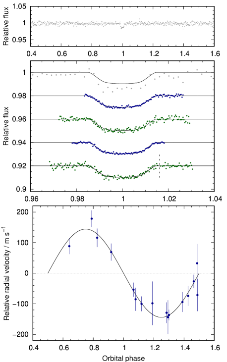
Figure 4: WASP-146b discovery data. As for Fig. 2.

We obtained lightcurves from the time-series images using standard differential aperture photometry (second panel of Figs. 1, 2, 3 and 4). We computed radial-velocity (RV) measurements from the CORALIE and HARPS spectra by weighted cross-correlation with a G2 binary mask (Baranne et al., 1996; Pepe et al., 2002). We detected sinusoidal variations in the RVs with semi-amplitudes consistent with planetary mass companions and that phase with the WASP ephemerides (bottom panel of Figs. 1, 2, 3 and 4). The lack of correlation between RV and bisector span supports our conclusion that the RV signals are induced by orbiting bodies and not by stellar activity (Fig. 5; Queloz et al. 2001).

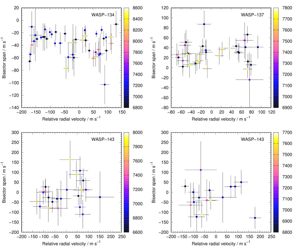
Figure 5: Bisector span versus radial velocity. The colour bar depicts the Barycentric Julian Date (BJD-2450000). For WASP-134, we omit the HARPS data taken through the transits as they will be affected by the RM effect.

3 Stellar analysis

We performed spectral analyses using the procedures detailed in Doyle et al. (2013) to obtain stellar effective temperature $T_{\rm eff}$, surface gravity $\log g_{*}$, metallicity [Fe/H], projected rotation speed $v\sin i_{\rm*,spec}$, and lithium abundance $\log A({\rm Li})$. The results of the spectral analyses are given in Table 2. We calculated macroturbulence using the calibration of Doyle et al. (2014). We calculated distance using the Gaia DR2 parallax (Gaia Collaboration et al., 2018), and stellar luminosity and radius using the infrared flux method (IRFM) of Blackwell & Shallis (1977). Using the method of Maxted et al. (2011), we checked for modulation of the WASP lightcurves as can be caused by the combination of magnetic activity and stellar rotation. We find no signals with amplitudes greater than 1–2 mmag.

Though we can measure stellar density $\rho_{*}$ directly from the transit lightcurves, we require a constraint on stellar mass $M_{*}$ or radius $R_{*}$ for a full characterisation of the system. For each star we inferred $M_{*}$ and age $\tau$ using the bagemass stellar evolution MCMC code of Maxted et al. (2015), with input of the values of $\rho_{*}$ from initial MCMC analyses (see Section 2) and $T_{\rm eff}$ and [Fe/H] from the spectral analyses. We conservatively inflated the error bar by a factor of 2 to place Gaussian priors on $M_{*}$ in our final MCMC analyses. We note that the values of $R_{*}$ from our final MCMC analyses are consistent with the values obtained from the IRFM and the Gaia parallax (compare the values in Tables 2 and 4).

Table 2: Stellar parameters

Parameter	Symbol	WASP-134	WASP-137	WASP-143	WASP-146	Unit
Constellation	…	Pegasus	Cetus	Hydra	Aquarius	…
Right Ascension (J2000)	…	$\rm 21^{h}50^{m}16\fs 77$	$\rm 01^{h}43^{m}29\fs 09$	$\rm 09^{h}23^{m}22\fs 96$	$\rm 23^{h}56^{m}22\fs 02$	…
Declination (J2000)	…	$\rm+04\arcdeg 11\arcmin 40\fs 3$	$\rm-14\arcdeg 08\arcmin 56\fs 8$	$\rm+02\arcdeg 55\arcmin 57\fs 1$	$\rm-13\arcdeg 16\arcmin 17\fs 6$	…
Tycho-2 $V_{\rm mag}$	$V$	11.3	11.0	12.6	12.9	…
2MASS $K_{\rm mag}$	$K$	9.4	9.5	11.3	11.0	…
Spectral type	…	G4	G0	G1	G0	…
Stellar effective temperature	$T_{\rm eff}$	5700 $\pm$ 100	6100 $\pm$ 140	5900 $\pm$ 140	6100 $\pm$ 140	K
Distance (Gaia)	d	$195\pm 2$	$289\pm 4$	$402\pm 7$	$495\pm 27$	pc
Stellar mass	$M_{*}$	$1.131\pm 0.045$	$1.216\pm 0.066$	$1.087\pm 0.045$	$1.057\pm 0.085$	$M_{\odot}$
Stellar radius (IRFM)	$R_{\rm*,IRFM}$	$1.16\pm 0.06$	$1.65\pm 0.10$	$1.00\pm 0.05$	$1.29\pm 0.06$	$R_{\odot}$
Stellar surface gravity	$\log g_{*}$	4.4 $\pm$ 0.1	4.0 $\pm$ 0.2	4.4 $\pm$ 0.2	4.3 $\pm$ 0.2	[cgs]
Stellar metallicity	[Fe/H]	$+0.40\pm 0.07$	$+0.08\pm 0.07$	$+0.23\pm 0.10$	$-0.01\pm 0.16$	…
Stellar luminosity	$\log(L/L_{\odot})$	0.103 $\pm$ 0.048	0.487 $\pm$ 0.051	0.027 $\pm$ 0.041	0.268 $\pm$ 0.044	…
Proj. stellar rotation speed	$v\sin i_{\rm*,spec}$	$0.9\pm 0.6$	$3.7\pm 0.9$	$0.9\pm 0.9$	$0.9\pm 0.9$	km  s-1
Lithium abundance	$\log A({\rm Li})$	$<0.4$	$2.87\pm 0.08$	$<1.6$	$<1.6$	…
Macroturbulence	$v_{\rm mac}$	3.1	5.0	3.6	3.8	km  s-1
Age	$\tau$	$5.1\pm 1.6$	$4.3\pm 1.8$	$1.9\pm 1.5$	$6.9\pm 2.5$	Gyr

sectionSystem parameters from MCMC analyses We determined the system parameters from a simultaneous fit to the transit lightcurves and the radial velocities using the current version of the Markov-chain Monte Carlo (MCMC) code presented in Collier Cameron et al. (2007) and described further in Anderson et al. (2015b). We partitioned those TRAPPIST-South lightcurves affected by meridian flips so as to account for any offsets. When fitting eccentric orbits, we obtained $e=0.076\pm 0.032$ for WASP-137b, $e=0.0021^{+0.0014}_{-0.0007}$ for WASP-143b, and $e=0.041^{+0.049}_{-0.029}$ for WASP-146b. Each value is small and of low significance, so we adopted circular orbits, as is encouraged by Anderson et al. (2012) for hot Jupiters in the absence of evidence to the contrary.

We adopted an eccentric orbit for WASP-134b ($P$ = 10.1 d) as it fits the data much better than does a circular orbit ($\rm\Delta AICc=40$). Having noticed excess scatter about an initial fit, we calculated a periodogram of the residuals and found a significant peak around $P$ = 70 d (Fig. 6, top panel; FAP $<$ 0.001), which we attribute to the planet WASP-134c. The absence of a correlation between bisector span and residual RV (about the best-fitting orbit for WASP-134b) supports our interpretation that the 70-d signal is induced by a planet and not stellar activity (Fig. 6, middle panel). We used the RadVel code of Fulton et al. (2018) to fit a two-planet model, fixing $P$ and $T_{\rm c}$ for the inner planet at the values derived from the transit photometry, placing a limit on eccentricity of $e<0.35$, and excluding the transit sequences. We plot the best-fitting two-planet model in Fig. 7 and provide the two-planet solution in Table 3. The two-planet model is a much better fit to the data than is the one-planet model ($\rm\Delta AICc=111$). A periodogram of the residual RVs about the two-planet model shows no significant peak (Fig. 6, bottom panel). We do not see evidence of transits of WASP-134c in the WASP data, but the phase coverage is sparse (only a few transits of WASP-134b had good coverage). TESS is scheduled to observe WASP-134 during 2019 Aug 15 to 2019 Sep 11 (camera 1, Sector 15), whereas we predict the nearby inferior conjunctions of WASP-134c to occur on 2019 Aug 8 and 2019 Oct 17, with a 1-$\sigma$ uncertainty of 5 d. We subtracted the best-fitting orbit of WASP-134c from the RVs of WASP-134 prior to the MCMC analysis.

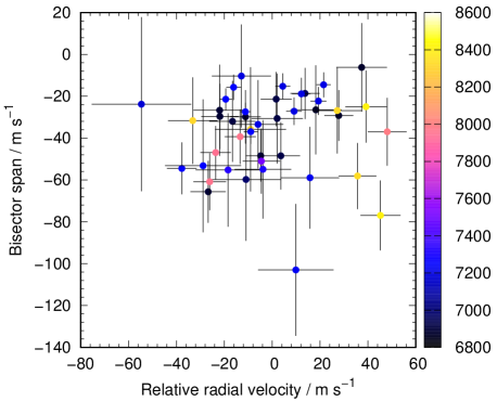
Figure 6: The evidence for WASP-134c. Top panel: The periodogram of the residual RVs of WASP-134 after subtraction of the motion due to WASP-134b ($P=10.15$ d). The horizontal lines indicate the 10, 1 and 0.1 per cent false-alarm levels. The peak around 70 d, which we attribute to the planet WASP-134c, has a false-alarm probability of FAP $<$ 0.001. Middle panel: Bisector span versus residual RV of WASP-134 after subtraction of the motion due to WASP-134b. The colour bar depicts the Barycentric Julian Date (BJD-2450000). Bottom panel: The periodogram of the residual RVs of WASP-134 after subtraction of the motion due to both WASP-134b and WASP-134c ($P=70.0$ d).

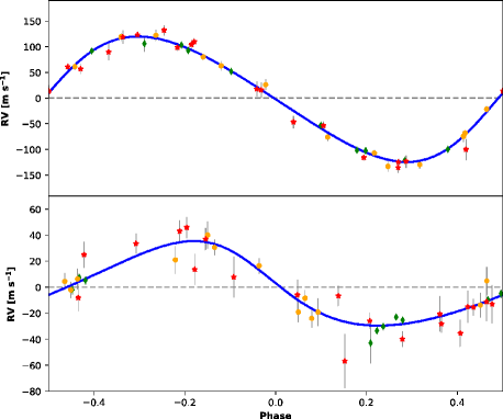
Figure 7: A two-planet fit to the RVs of WASP-134 (excluding the transit sequences). Top panel: The phase-folded orbit of WASP-134b ($P=10.15$ d). Bottom panel: The phase-folded orbit of WASP-134c ($P=70.0$ d). The CORALIE07 and CORALIE14 RVs are shown as yellow circles and red stars, respectively. The HARPS-S RVs are shown as green diamonds.

Table 3: Two-planet solution for WASP-134

Parameter	Symbol	WASP-134b	WASP-134c	Unit
Orbital period	$P$	10.1498 (fixed)	70.01 $\pm$ 0.14	d
Epoch of infer. conjunc.	$T_{\rm conj}$	2457464.848 (fixed)	2457234.2 $\pm$ 1.8	d
Orbital eccentricity	$e$	0.146 $\pm$ 0.015	$0.173\pm 0.090$	…
Arg. of periastron	$\omega$	$-97.2\pm 2.6$	$58\pm 32$	∘
Refl. veloc. semi-ampl.	$K_{\rm 1}$	122.1 $\pm$ 2.1	32.5 $\pm$ 2.7	km  s-1
Minimum planet mass	$M_{\rm P}$ $\sin i$	$1.40\pm 0.08$	$0.70\pm 0.07$	$M_{\rm Jup}$

For each system, to for instrumental and astrophysical offsets, we partitioned the RV datasets and fit a separate systemic velocity to each of them. This included the CORALIE RVs from before and after the November 2014 upgrade (labelled CORALIE07 and CORALIE14, respectively), and the HARPS RVs around the orbit and through the transits of WASP-134b.

For WASP-134b, we modelled the Rossiter-McLaughlin (RM) effect using the formulation of Hirano et al. (2011). Due to the low transit impact parameter, there is a degeneracy between the projected stellar rotation speed $v\sin i_{\rm*,RM}$ and the projected stellar obliquity $\lambda$ (e.g. Albrecht et al. 2011). This results in values of $v\sin i_{\rm*,RM}$ ($>$ 9 km  s^-1) far higher than the value from our spectral analysis ($v\sin i_{\rm*,spec}=0.9\pm 0.6$ km  s^-1), so we placed a Gaussian prior on $v\sin i_{\rm*,RM}$ using the value from the spectral analysis. With the prior, we obtained $\lambda=-43.7\pm 9.9^{\circ}$ and $v\sin i_{\rm*,RM}=2.08\pm 0.26$ km  s^-1. Without the prior, we obtained $\lambda=-67^{+15}_{-9}$^∘ and $v\sin i_{\rm*,RM}=3.3^{+1.5}_{-0.9}$ km  s^-1.

We present the median values and 1-$\sigma$ limits on the system parameters from our final MCMC analyses in Table 4. We plot the best fits to the RVs and the transit lightcurves in Figs. 1, 2, 3 and 4 and the residuals of the RVs about the best-fitting orbital models in Fig. 8.

Table 4: System parameters

Parameter	Symbol	WASP-134	WASP-137	WASP-143	WASP-146	Unit
MCMC Gaussian priors
Stellar mass	$M_{\rm*}$	1.13 $\pm$ 0.09	1.22 $\pm$ 0.13	1.087 $\pm$ 0.090	1.06 $\pm$ 0.17	$M_{\rm\odot}$
Stellar effective temperature	$T_{\rm eff}$	5700 $\pm$ 100	6100 $\pm$ 140	5900 $\pm$ 1400	5900 $\pm$ 140	K
MCMC parameters controlled by Gaussian priors
Stellar mass	$M_{\rm*}$	1.130 $\pm$ 0.091	1.22 $\pm$ 0.13	1.096 $\pm$ 0.091	1.06 $\pm$ 0.17	$M_{\rm\odot}$
Stellar effective temperature	$T_{\rm eff}$	5574 $\pm$ 99	6127 $\pm$ 136	6042 $\pm$ 135	5894 $\pm$ 140	K
MCMC fitted parameters
Orbital period	$P$	10.1467583 $\pm$ 0.0000080	3.9080284 $\pm$ 0.0000053	3.7788730 $\pm$ 0.0000032	3.3969440 $\pm$ 0.0000036	d
Transit epoch (HJD)	$T_{\rm c}$	2457201.03099 $\pm$ 0.00075	2456937.61342 $\pm$ 0.00106	2457099.94471 $\pm$ 0.00015	2457109.72182 $\pm$ 0.00021	d
Transit duration	$T_{\rm 14}$	0.2218 $\pm$ 0.0019	0.1425 $\pm$ 0.0034	0.12858 $\pm$ 0.00055	0.09980 $\pm$ 0.00097	d
Planet-to-star area ratio	$R_{\rm P}^{2}$/R${}_{*}^{2}$	0.00749 $\pm$ 0.00020	0.00737 $\pm$ 0.00031	0.01569 $\pm$ 0.00017	0.01049 $\pm$ 0.00017	…
Impact parameter	$b$	0.306 $\pm$ 0.082	0.690 $\pm$ 0.049	0.181 $\pm$ 0.097	0.8290 $\pm$ 0.0089	…
Reflex velocity semi-amplitude	$K_{\rm 1}$	0.1220 $\pm$ 0.0012	0.0767 $\pm$ 0.0026	0.0890 $\pm$ 0.0085	0.144 $\pm$ 0.012	km  s-1
Systemic velocity (CORALIE07)	$\gamma_{\rm CORALIE07}$	5.7967 $\pm$ 0.0021	4.6948 $\pm$ 0.0027	20.215 $\pm$ 0.010	$-$5.6464 $\pm$ 0.0084	km  s-1
Systemic velocity (CORALIE14)	$\gamma_{\rm CORALIE14}$	5.7975 $\pm$ 0.0020	4.6937 $\pm$ 0.0022	20.2008 $\pm$ 0.0088	$-$5.6144 $\pm$ 0.015	km  s-1
Systemic velocity (HARPS-S)	$\gamma_{\rm HARPS-S}$	5.82223 $\pm$ 0.00097	…	…	…	km  s-1
Systemic velocity (HARPS-S RM)	$\gamma_{\rm HARPS-S_{\rm RM}}$	5.8200 $\pm$ 0.0015	…	…	…	km  s-1
Systemic velocity (HARPS-N RM)	$\gamma_{\rm HARPS-N_{\rm RM}}$	5.83155 $\pm$ 0.00048	…	…	…	km  s-1
First eccentricity parameter	$e\cos\omega$	$-0.0187\pm 0.0042$	…	…	…
Second eccentricity parameter	$e\sin\omega$	$-0.1435\pm 0.0086$	…	…	…
First obliquity parameter	$v_{*}\sin i_{*}\cos\lambda$	$1.49\pm 0.20$	…	…	…
Second obliquity parameter	$v_{*}\sin i_{*}\sin\lambda$	$-1.42\pm 0.39$	…	…	…
MCMC derived parameters
Orbital eccentricity	$e$	0.1447 $\pm$ 0.0086 ($<$ 0.16 at 2$\sigma$)	0 ($<$ 0.14 at 2$\sigma$)	0 ($<$ 0.0007 at 2$\sigma$)	0 ($<$ 0.15 at 2$\sigma$)	…
Argument of periastron	$\omega$	$-97.4\pm 1.7$	…	…	…	∘
Sky-projected stellar obliquity	$\lambda$	$-$43.7 $\pm$ 9.9	…	…	…	∘
Sky-projected stellar rotation speed	$v\sin i_{\rm*,RM}$	2.08 $\pm$ 0.26	…	…	…	km  s-1
Scaled semi-major axis	$a/R_{\rm*}$	$17.53\pm 0.53$	$7.31\pm 0.47$	$10.39\pm 0.17$	$7.88\pm 0.16$	…
Orbital inclination	$i$	89.13 $\pm$ 0.26	84.59 $\pm$ 0.73	89.00 $\pm$ 0.55	83.96 $\pm$ 0.19	∘
Ingress and egress duration	$T_{\rm 12}=T_{\rm 34}$	0.0193 $\pm$ 0.0013	0.0203 $\pm$ 0.0030	0.01473 $\pm$ 0.00056	0.0263 $\pm$ 0.0015	d
Stellar radius	$R_{\rm*}$	$1.175\pm 0.048$	1.52 $\pm$ 0.11	1.013 $\pm$ 0.032	1.232 $\pm$ 0.072	$R_{\rm\odot}$
Stellar surface gravity	$\log g_{*}$	4.352 $\pm$ 0.029	4.155 $\pm$ 0.059	4.465 $\pm$ 0.018	4.282 $\pm$ 0.029	[cgs]
Stellar density	$\rho_{\rm*}$	0.702 $\pm$ 0.063	0.343 $\pm$ 0.066	1.054 $\pm$ 0.050	0.568 $\pm$ 0.035	$\rho_{\rm\odot}$
Planetary mass	$M_{\rm P}$	$1.412\pm 0.075$	0.681 $\pm$ 0.054	0.725 $\pm$ 0.084	1.11 $\pm$ 0.15	$M_{\rm Jup}$
Planetary radius	$R_{\rm P}$	0.988 $\pm$ 0.057	1.27 $\pm$ 0.11	1.234 $\pm$ 0.042	1.228 $\pm$ 0.076	$R_{\rm Jup}$
Planetary surface gravity	$\log g_{\rm P}$	3.521 $\pm$ 0.034	2.983 $\pm$ 0.069	3.033 $\pm$ 0.045	3.229 $\pm$ 0.044	[cgs]
Planetary density	$\rho_{\rm P}$	1.47 $\pm$ 0.18	0.333 $\pm$ 0.081	0.382 $\pm$ 0.045	0.604 $\pm$ 0.084	$\rho_{\rm J}$
Orbital semi-major axis	$a$	0.0956 $\pm$ 0.0025	0.0519 $\pm$ 0.0018	0.0490 $\pm$ 0.0014	0.0451 $\pm$ 0.0024	AU
Planetary equilibrium temperature	$T_{\rm eql}$	953 $\pm$ 22	1601 $\pm$ 65	1325 $\pm$ 30	1486 $\pm$ 43	K

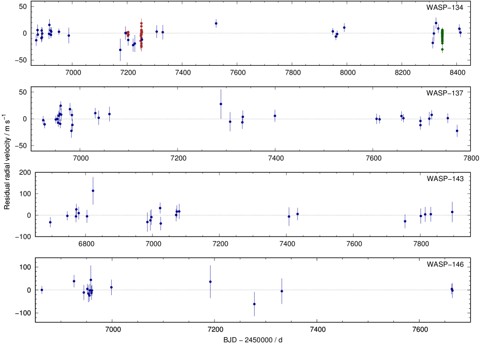
Figure 8: The residual RVs about the best-fitting orbital and RM effect models. The symbol colours are the same as in Fig. 1.

4 Discussion

We have presented the discovery of five Jupiter-mass planets ($M_{\rm P}$ = 0.68–1.41 $M_{\rm Jup}$) orbiting moderately bright ($V$ = 11.0–12.9) Solar-type stars ($M_{*}$ = 1.06–1.22 $M_{\odot}$). As fairly typical hot Jupiters ($T_{\rm eql}$ = 1300–1600 K) with orbital periods of $P$ = 3–4 d, WASP-137b, WASP-143b and WASP-146b are remarkably similar to each other (Tables 2 and 4).

The WASP-134 system is rather more interesting. WASP-134 is a metal-rich G4 star ([Fe/H] = +0.40 $\pm$ 0.07) orbited by two warm Jupiters. WASP-134b ($M_{\rm P}$ = 1.41 $M_{\rm Jup}$; $T_{\rm eql}$ = 950 K) is in an eccentric ($e=0.15\pm 0.01$), 10.15-d orbit ($a$ = 0.096 AU) that is misaligned with the spin of the star ($\lambda=-44\pm 10^{\circ}$). Its companion, WASP-134c ($M_{\rm P}$ $\sin i$ = 0.70 $M_{\rm Jup}$; $T_{\rm eql}$ = 500 K), is in an eccentric ($e=0.17\pm 0.09$), 70.0-d orbit ($a$ = 0.35 AU). Thus WASP-134 is a rare type of system: a hot/warm Jupiter with a nearby giant companion. In that respect, WASP-134 may be similar to the HAT-P-46 system. Hartman et al. (2014) found that their RVs of HAT-P-46 are fit well with a two-planet model: $M_{\rm P}$ = 0.49 and $P=4.5$ d for HAT-P-46b and $M_{\rm P}$ $\sin i$ = 2.0 $M_{\rm Jup}$ and $P=78$ d for the candidate planet HAT-P-46c. The evidence for HAT-P-46c, though, is not yet conclusive and further RV monitoring is required.

Of those hot/warm Jupiters with confirmed giant companions, the companions tend to be very far out (e.g. HAT-P-17c with $P=1610$ d; Howard et al. 2012), and rarely closer than 1 AU (e.g. WASP-41c at $a=1.07$ AU and WASP-47c at $a=1.36$ AU; Neveu-VanMalle et al. 2016). Also of note are those hot-Jupiter systems with brown-dwarf companions within a few AU, such as WASP-53 and WASP-81 (Triaud et al., 2017). In their tabulation of hot and warm Jupiters with nearby giant companions, Antonini et al. (2016) list only three companions inside of 1 AU, the closest of which is HD 9446 c at 0.65 AU (Hébrard et al., 2010). With $a=0.35$ AU, WASP-134c is in a much shorter orbit.

It seems unlikely that WASP-134b could have arrived in situ via high-eccentricity migration (e.g Petrovich & Tremaine 2016). Antonini et al. (2016) studied the observed population of hot and warm Jupiters with nearby giant companions and found that the ejection of a planet or its collision with the star are more likely outcomes when exploring such pathways. Thus in-situ formation (e.g. Huang et al. 2016) or disc migration (e.g. Lin et al. 1996) seem more likely explanations.

References

- Albrecht et al. (2011) Albrecht, S., Winn, J. N., Johnson, J. A., et al. 2011, ApJ, 738, 50, doi: 10.1088/0004-637X/738/1/50
- Anderson et al. (2012) Anderson, D. R., Collier Cameron, A., Gillon, M., et al. 2012, MNRAS, 422, 1988, doi: 10.1111/j.1365-2966.2012.20635.x
- Anderson et al. (2015a) Anderson, D. R., Triaud, A. H. M. J., Turner, O. D., et al. 2015a, ApJ, 800, L9, doi: 10.1088/2041-8205/800/1/L9
- Anderson et al. (2015b) Anderson, D. R., Collier Cameron, A., Hellier, C., et al. 2015b, A&A, 575, A61, doi: 10.1051/0004-6361/201423591
- Antonini et al. (2016) Antonini, F., Hamers, A. S., & Lithwick, Y. 2016, AJ, 152, 174, doi: 10.3847/0004-6256/152/6/174
- Asplund et al. (2009) Asplund, M., Grevesse, N., Sauval, A. J., & Scott, P. 2009, ARA&A, 47, 481, doi: 10.1146/annurev.astro.46.060407.145222
- Bakos (2018) Bakos, G. Á. 2018, The HATNet and HATSouth Exoplanet Surveys, 111
- Baranne et al. (1996) Baranne, A., Queloz, D., Mayor, M., et al. 1996, A&AS, 119, 373
- Becker et al. (2015) Becker, J. C., Vanderburg, A., Adams, F. C., Rappaport, S. A., & Schwengeler, H. M. 2015, ApJ, 812, L18, doi: 10.1088/2041-8205/812/2/L18
- Blackwell & Shallis (1977) Blackwell, D. E., & Shallis, M. J. 1977, MNRAS, 180, 177
- Broeg et al. (2013) Broeg, C., Fortier, A., Ehrenreich, D., et al. 2013, in European Physical Journal Web of Conferences, Vol. 47, European Physical Journal Web of Conferences, 03005
- Collier Cameron et al. (2006) Collier Cameron, A., Pollacco, D., Street, R. A., et al. 2006, MNRAS, 373, 799, doi: 10.1111/j.1365-2966.2006.11074.x
- Collier Cameron et al. (2007) Collier Cameron, A., Wilson, D. M., West, R. G., et al. 2007, MNRAS, 380, 1230, doi: 10.1111/j.1365-2966.2007.12195.x
- Cooke et al. (2018) Cooke, B. F., Pollacco, D., West, R., McCormac, J., & Wheatley, P. J. 2018, A&A, 619, A175, doi: 10.1051/0004-6361/201834014
- Cosentino et al. (2012) Cosentino, R., Lovis, C., Pepe, F., et al. 2012, in Society of Photo-Optical Instrumentation Engineers (SPIE) Conference Series, Vol. 8446, Society of Photo-Optical Instrumentation Engineers (SPIE) Conference Series
- Delrez et al. (2018) Delrez, L., Gillon, M., Queloz, D., et al. 2018, in Society of Photo-Optical Instrumentation Engineers (SPIE) Conference Series, Vol. 10700, Ground-based and Airborne Telescopes VII, 107001I
- Doyle et al. (2014) Doyle, A. P., Davies, G. R., Smalley, B., Chaplin, W. J., & Elsworth, Y. 2014, MNRAS, 444, 3592, doi: 10.1093/mnras/stu1692
- Doyle et al. (2013) Doyle, A. P., Smalley, B., Maxted, P. F. L., et al. 2013, MNRAS, 428, 3164, doi: 10.1093/mnras/sts267
- Fulton et al. (2018) Fulton, B. J., Petigura, E. A., Blunt, S., & Sinukoff, E. 2018, PASP, 130, 044504, doi: 10.1088/1538-3873/aaaaa8
- Gaia Collaboration et al. (2018) Gaia Collaboration, Brown, A. G. A., Vallenari, A., et al. 2018, A&A, 616, A1, doi: 10.1051/0004-6361/201833051
- Gillon et al. (2011) Gillon, M., Jehin, E., Magain, P., et al. 2011, Detection and Dynamics of Transiting Exoplanets, St. Michel l’Observatoire, France, Edited by F. Bouchy; R. Díaz; C. Moutou; EPJ Web of Conferences, Volume 11, id.06002, 11, 6002, doi: 10.1051/epjconf/20101106002
- Gray (1992) Gray, D. F. 1992, The observation and analysis of stellar photospheres.
- Hartman et al. (2014) Hartman, J. D., Bakos, G. Á., Torres, G., et al. 2014, AJ, 147, 128, doi: 10.1088/0004-6256/147/6/128
- Hébrard et al. (2010) Hébrard, G., Bonfils, X., Ségransan, D., et al. 2010, A&A, 513, A69, doi: 10.1051/0004-6361/200913790
- Hellier et al. (2012) Hellier, C., Anderson, D. R., Collier Cameron, A., et al. 2012, MNRAS, 426, 739, doi: 10.1111/j.1365-2966.2012.21780.x
- Hirano et al. (2011) Hirano, T., Suto, Y., Winn, J. N., et al. 2011, ApJ, 742, 69, doi: 10.1088/0004-637X/742/2/69
- Howard et al. (2012) Howard, A. W., Bakos, G. Á., Hartman, J., et al. 2012, ApJ, 749, 134, doi: 10.1088/0004-637X/749/2/134
- Huang et al. (2016) Huang, C., Wu, Y., & Triaud, A. H. M. J. 2016, ApJ, 825, 98, doi: 10.3847/0004-637X/825/2/98
- Jehin et al. (2011) Jehin, E., Gillon, M., Queloz, D., et al. 2011, The Messenger, 145, 2
- Lendl et al. (2012) Lendl, M., Anderson, D. R., Collier-Cameron, A., et al. 2012, A&A, 544, A72, doi: 10.1051/0004-6361/201219585
- Lin et al. (1996) Lin, D. N. C., Bodenheimer, P., & Richardson, D. C. 1996, Nature, 380, 606, doi: 10.1038/380606a0
- Maxted et al. (2015) Maxted, P. F. L., Serenelli, A. M., & Southworth, J. 2015, A&A, 575, A36, doi: 10.1051/0004-6361/201425331
- Maxted et al. (2011) Maxted, P. F. L., Anderson, D. R., Collier Cameron, A., et al. 2011, PASP, 123, 547, doi: 10.1086/660007
- Neveu-VanMalle et al. (2016) Neveu-VanMalle, M., Queloz, D., Anderson, D. R., et al. 2016, A&A, 586, A93, doi: 10.1051/0004-6361/201526965
- Pepe et al. (2002) Pepe, F., Mayor, M., Rupprecht, G., et al. 2002, The Messenger, 110, 9
- Pepper et al. (2007) Pepper, J., Pogge, R. W., DePoy, D. L., et al. 2007, PASP, 119, 923, doi: 10.1086/521836
- Petrovich & Tremaine (2016) Petrovich, C., & Tremaine, S. 2016, ApJ, 829, 132, doi: 10.3847/0004-637X/829/2/132
- Pollacco et al. (2006) Pollacco, D. L., Skillen, I., Cameron, A. C., et al. 2006, PASP, 118, 1407, doi: 10.1086/508556
- Queloz et al. (2000) Queloz, D., Mayor, M., Weber, L., et al. 2000, A&A, 354, 99
- Queloz et al. (2001) Queloz, D., Henry, G. W., Sivan, J. P., et al. 2001, A&A, 379, 279, doi: 10.1051/0004-6361:20011308
- Ricker et al. (2014) Ricker, G. R., Winn, J. N., Vanderspek, R., et al. 2014, in Proc. SPIE, Vol. 9143, Space Telescopes and Instrumentation 2014: Optical, Infrared, and Millimeter Wave, 914320
- Santerne et al. (2016) Santerne, A., Moutou, C., Tsantaki, M., et al. 2016, A&A, 587, A64, doi: 10.1051/0004-6361/201527329
- Southworth (2011) Southworth, J. 2011, MNRAS, 417, 2166, doi: 10.1111/j.1365-2966.2011.19399.x
- Triaud et al. (2017) Triaud, A. H. M. J., Neveu-VanMalle, M., Lendl, M., et al. 2017, MNRAS, 467, 1714, doi: 10.1093/mnras/stx154
- Wheatley et al. (2018) Wheatley, P. J., West, R. G., Goad, M. R., et al. 2018, MNRAS, 475, 4476, doi: 10.1093/mnras/stx2836
- Yao et al. (2018) Yao, X., Pepper, J., Gaudi, B. S., et al. 2018, ArXiv e-prints. https://arxiv.org/abs/1807.11922