Analytical solution for magnetized thin accretion disk in comparison with numerical simulations

Abstract

We obtained equations for a thin magnetic accretion disk, using the method of asymptotic approximation. They cannot be solved analytically-without solutions for a magnetic field in the magnetosphere between the star and the disk, only a set of general conditions on the solutions can be derived. To compare the analytical results with numerical solutions, we find expressions for physical quantities in the disk, using our results from resistive and viscous star-disk magnetospheric interaction simulations.

1 Introduction

Gravitational infall of matter onto a rotating central object naturally forms a rotating accretion disk. Matter from the disk is then fed inwards through an accretion column. Examples of single objects with a disk around them are protostars and young stellar objects, and in close binary systems a disk can form when matter from donor star falls onto a white dwarf or a neutron star.

Analytical hydro-dynamical model of a thin accretion disk, with viscosity parameterized by Shakura & Sunyaev $\alpha$-prescription, has been given in [Kluźniak & Kita (2000), Kluźniak & Kita (2000)]. We extend this model, obtaining the equations for a magnetic thin disk. Analytical solution in the magnetic case cannot be given without knowing the solutions in a star-disk magnetosphere, only general conditions on solutions could be derived.

We perform numerical simulations of star-disk magnetospheric interaction, adding a stellar rotating surface and a magnetic field to the analytical hydro-dynamical disk solution used as an initial condition in simulations. A quasi-stationary solution is obtained, from which we find simple matching expressions for physical quantities in the disk. Those expressions can be compared with requirements from the analytically obtained equations for the magnetic disk and with the hydro-dynamic analytical and numerical solutions.

Figure 1: A zoom into our simulation result after T=80 rotations of the underlying star. Shown is the density in logarithmic color grading in code units, with a sample of magnetic field lines, depicted with white solid lines. Velocities in the disk, column and stellar wind are shown with vectors, depicted in different normalizations with respect to the Keplerian velocity at the stellar surface.

2 Numerical setup

We use the publicly available pluto code (v.4.1) ([Mignone et al.(2007), Mignone et al.(2012), Mignone et al. 2007; 2012]), with logarithmically stretched grid in radial direction in spherical coordinates, and uniformly spaced latitudinal grid. Resolution is $R\times\theta$=[$217\times 100$] grid cells, stretching the domain to 30 stellar radii. We perform axisymmetric 2D star-disk simulations in resistive and viscous magneto-hydrodynamics, following [Zanni & Ferreira (2009), Zanni & Ferreira (2009)] - see also [Čemeljić et al. (2017), Čemeljić et al. (2017)].

The equations solved by the pluto code are, in the cgs units:

$$\frac{\partial\rho}{\partial t}+\nabla\cdot(\rho\mathbf{v})=0$$

$$\frac{\partial\rho\mathbf{v}}{\partial t}+\nabla\cdot\left[\rho\mathbf{v}\mathbf{v}+\left(P+\frac{\mathbf{B}\mathbf{B}}{8\pi}\right)\mathbf{I}-\frac{\mathbf{B}\mathbf{B}}{4\pi}-\mathbf{\tau}\right]=\rho\mathbf{g}$$

$$\frac{\partial E}{\partial t}+\nabla\cdot\left[\left(E+P+\frac{\mathbf{B}\mathbf{B}}{8\pi}\right)\mathbf{v}+\underbrace{\eta_{\rm m}\mathbf{J}\times\mathbf{B}/4\pi-\mathbf{v}\cdot\mathbf{\tau}}_{\rm heating\ terms}\right]=\rho\mathbf{g}\cdot\mathbf{v}-\underbrace{{\Lambda}}_{\rm cooling}$$

$$\frac{\partial\mathbf{B}}{\partial t}+\nabla\times(\mathbf{B}\times\mathbf{v}+\eta_{\rm m}\mathbf{J})=0.$$

Symbols have their usual meaning. The underbraced Ohmic and viscous heating terms and the cooling term are removed in our computations, to prevent the thermal thickening of the accretion disk. This equals the assumption that all the heating is radiated away from the disk. The solutions are still in a non-ideal magneto-hydrodynamics regime, because of the viscous term in the momentum equation, and the resistive term in the induction equation.

3 Analytical solutions ver. numerical solutions

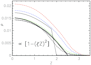
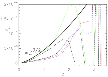
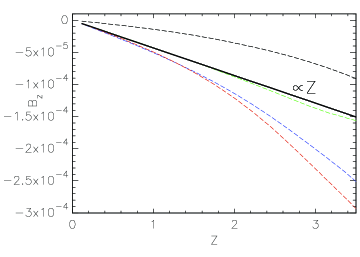
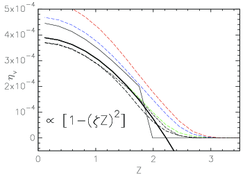
Figure 2: Trends with the increasing stellar magnetic strength in the disk density, velocity, magnetic field and viscosity. The values are taken at R=15R_⋆ in the vertical direction, with Z expressed in the units of R_⋆. With the thin solid line is shown the KK00 solution, with the dash-dotted line is shown the solution without the magnetic field, and in black, green, blue and green dashed lines are shown the solutions with $B_{\star}$=0.025, 0.05, 0.075 and 0.1 T, respectively. With the thick solid line is shown a match to the $B_{\star}$=0.05 T case. Expressions for the match in B_⋆=0.05 T case are written in each panel, with $\zeta$ in the density equal to 0.4, and in the viscosity to 0.45. The density, velocity, dynamic viscosity and magnetic field are expressed in the code units $\rho_{\rm d0}$=$\dot{M}_{0}/(R_{\star}^{2}v_{\rm K\star})$, $v_{0}=v_{\rm K\star}$, $\eta_{\rm v0}=\rho_{\rm d0}R_{\star}v_{\rm K\star}$, and $B_{0}=v_{\rm K\star}\sqrt{\rho_{\rm d0}}$, where $\dot{M}_{0}$ is the free parameter in the simulations, denoting the disk accretion rate, and $v_{\rm K\star}$ is the Keplerian velocity at the stellar surface.

Table 1: Coefficients k in the expressions from results in our simulation with $B_{\star}$=0.05 T.

$k_{1}$	$k_{2}$	$k_{3}$	$k_{4}$	$k_{5}$	$k_{6}$	$k_{7}$	$k_{8}$	$k_{9}$
0.88	-0.09	3.8$\times 10^{-5}$	0.255	-0.4	-0.15	-1.11	0.006	0.01

We extended the asymptotic approximation from a hydro-dynamic [Kluźniak & Kita (2000), Kluźniak & Kita (2000)] thin accretion disk solution to a magnetic case. Without knowing the solution for a magnetic field in a star-disk magnetosphere, which is connected with the solution in the disk, obtained equations cannot be solved analytically. In addition to the solutions which remain the same as in the hydro-dynamical case, only general constraints on the magnetic solution could be derived.

We compare the obtained analytical solutions and constraints in the magnetic case with the results from simulations. To do this, we write the solutions from simulations in terms of matching expressions-which are not formal fits, but simple matching functions chosen to represent the result within 10% of the value from the simulation, when there is no oscillations. In all the cases, the match is chosen to the solution in the middle of the disk, further away from the star than the corotation radius, where the disk co-rotates with the star, which is at $R_{\rm cor}=2.9R_{\star}$.

We confirm that in the middle part of the disk, at R=15R_⋆, the numerical solution in the magnetic case does not differ much from the hydro-dynamical analytical and numerical solutions. The difference is only in the proportionality coefficients $k$ in the expressions for physical quantities and in the corresponding power laws.

The expressions we obtain are:

$$\rho(r,z)=\frac{k_{1}}{r^{3/2}}[1-(0.4z)^{2}],$$

$$v_{r}(r,z)=\frac{k_{2}}{r^{3/2}}[1+(0.5z)^{2}],\ v_{z}(r,z)=\frac{k_{3}}{r}z^{3/2},\ v_{\varphi}(r,z)=\frac{k_{4}}{\sqrt{r}},$$

$$B_{r}(r,z)=\frac{k_{5}}{r^{3}}z,\ B_{z}(r,z)=\frac{k_{6}}{r^{3}}z,\ B_{\varphi}(r,z)=\frac{k_{7}}{r^{3}}z,$$

$$\eta(r,z)=\frac{k_{8}}{r}[1-(0.45z)^{2}],\ \eta_{\rm m}(r,z)=k_{9}\sqrt{r}[1-(0.3z)^{2}].$$

We tabulate the coefficients $k$ in the case of a Young Stellar Object rotating with $\Omega_{\star}=0.2$ of the breakup angular velocity, with the stellar field B_⋆=0.05 T, anomalous viscosity and resistivity coefficients $\alpha_{\rm v}$=1 and $\alpha_{\rm m}=1$, in Table 1.

In Fig. 2 we show the trends in the density, viscosity and vertical velocity and magnetic field components in the disk, in the cases with increasing stellar magnetic field strength.

4 Conclusions

We present our results in numerical simulations of a star-disk system with magnetospheric interaction in the case of Young Stellar Object with the stellar field of 0.05 T, rotating with 20% of the breakup velocity. Quasi-stationary solutions in the disk are obtained, and we find simple expressions to match the physical quantities.

We find that the expressions in the magnetic cases differ from the results in the hydro-dynamical simulation and in the analytical solution only in proportionality coefficients.

In future work we will compare the trends in numerical solutions in the cases with different stellar magnetic field strength, rotation rate, viscosity and resistivity.