Spatially Random Relay Selection for Full/Half-Duplex Cooperative NOMA Networks

Abstract

This paper investigates the impact of relay selection (RS) on the performance of cooperative non-orthogonal multiple access (NOMA), where relays are capable of working in either full-duplex (FD) or half-duplex (HD) mode. A number of relays (i.e., $K$ relays) are uniformly distributed within the disc. A pair of RS schemes are considered insightfully: 1) Single-stage RS (SRS) scheme; and 2) Two-stage RS (TRS) scheme. In order to characterize the performance of these two RS schemes, new closed-form expressions for both exact and asymptotic outage probabilities are derived. Based on analytical results, the diversity orders achieved by the pair of RS schemes for FD/HD cooperative NOMA are obtained. Our analytical results reveal that: i) The FD-based RS schemes obtain a zero diversity order, which is due to the influence of loop interference (LI) at the relay; and ii) The HD-based RS schemes are capable of achieving a diversity order of $K$, which is equal to the number of relays. Finally, simulation results demonstrate that: 1) The FD-based RS schemes have better outage performance than HD-based RS schemes in the low signal-to-noise radio (SNR) region; 2) As the number of relays increases, the pair of RS schemes considered are capable of achieving the lower outage probability; and 3) The outage behaviors of FD/HD-based NOMA SRS/TRS schemes are superior to that of random RS (RRS) and orthogonal multiple access (OMA) based RS schemes.

I Introduction

With the rapid advancement in the wireless communication technology, the fifth generation (5G) mobile communication networks have attracted a great deal of attention [2, 3, 4]. In particular, three major families of new radio (NR) usage scenarios, i.e., massive machine type communications (mMTC), enhanced mobile broadband (eMBB) and ultra-reliable and low-latency communications (URLLC) are proposed to satisfy the different requirements for 5G networks. To improve system throughput and achieve enhanced spectrum efficiency of 5G networks, non-orthogonal multiple access (NOMA) has been considered to be a promising candidate technique and identified for 3GPP Long Term Evolution (LTE) [5]. The core idea of NOMA is able to multiplex additional users in the same physical resource. More specifically, the superposition coding scheme is employed at the transmitting end, where the linear superposition of signals of multiple users is formed to be the transmit signal. The successive interference cancellation (SIC) procedure is carried out by the receiving end who has the better channel conditions [6]. Furthermore, downlink multiuser superposition transmission scheme (MUST) [7] which is the special case of NOMA has found application in wireless standard.

Hence numerous excellent Contributions have surveyed the performance of point-to-point NOMA in wireless networks in [8, 9, 10, 11]. To evaluate the performance of downlink NOMA, the closed-form expressions of outage probability and ergodic rate for NOMA were derived in [8] by use of the bounded path loss model. Furthermore, the authors of [9] have studied the impact of user pairing on the performance of NOMA, where both the outage performance of fixed power allocation based NOMA (F-NOMA) and cognitive radio based NOMA (CR-NOMA) schemes were characterized. By considering user grouping and decoding order selection, the outage balancing among users was investigated [10], in which the closed-form expressions of optimal decoding order and power allocation for downlink NOMA were derived. In [11], the authors researched the outage behavior of downlink NOMA for the case where each NOMA user only feed back one bit of its channel state information (CSI) to a base station (BS). It was shown that NOMA is capable of providing higher fairness for multiple users compared to conventional opportunistic one-bit feedback. As a further advance, there is a paucity of research treaties on investigating the application of point-to-point NOMA systems. In [12], the authors analyzed the outage behavior of large-scale underlay CR for NOMA with the aid of stochastic geometry. To emphasize physical layer security (PLS), the authors in [13] discussed the PLS issues of NOMA, where the secrecy outage probabilities were derived for both single-antenna and multiple-antenna scenarios, respectively. Recently, the NOMA-based wireless cashing strategies were introduced in [14], in which two cashing phases, i.e., content pushing and content delivery, are characterized in terms of caching hit probability. Additionally, explicit insights for understanding the performance of uplink NOMA have been provided in [15, 16]. In [15], the novel uplink power control protocol was proposed for the single-cell uplink NOMA. In large-scale cellular networks, the performance of multi-cell uplink NOMA was characterized in terms of coverage probability using the theory of Poisson cluster process [16].

Cooperative communication is a promising approach to overcome signal fading arising from multipath propagation as well as obtain the higher diversity [17]. Obviously, combining cooperative communication technique and NOMA is the research topic which has sparked of wide interest in[18, 19, 20, 21]. The concept of cooperative NOMA was initially proposed for downlink transmission in [18], where the nearby user with better channel conditions was viewed as decode-and-forward (DF) relay to deliver the information for the distant users. Driven by these, authors in [19] analyzed the achievable data rate of NOMA systems for DF relay over Rayleigh fading channels. On the standpoint of tackling spectrum efficiency and energy efficiency, in [20], the application of simultaneous wireless information and power transfer (SWIPT) to NOMA with randomly deployed users was investigated using stochastic geometry. In [21], NOMA based dual-hop relay systems were addressed, where both statistical CSI and instantaneous CSI were considered for the networks. On the other hand, the outage performance of NOMA for a variable gain amplify-and-forward (AF) relay was characterized over Nakagami-$m$ fading channels in [22]. With the emphasis on imperfect CSI, authors studied the system outage behavior of AF relay for NOMA networks in [23]. Additionally, the authors of [24] analyzed the outage performance of a fixed gain based AF relay for NOMA systems over Nakagami-$m$ fading channels.

Above existing contributions on cooperative NOMA are all based on the assumption of half-duplex (HD) relay, where the communication process was completed in two slots [17]. To further improve the bandwidth usage efficiency of system, full-duplex (FD) relay technology is a promising solution which can simultaneously receive and transmit the signal in the same frequency band [25]. Nevertheless, FD operation suffers from residual loop self-interference (LI), which is usually modeled as a fading channel [26]. Particularly, FD relay technologies in [27] have been discussed from the view of self-interference cancellation, protocol design and relay selection for 5G networks. To maximize the weighted sum throughput of system, the design of resource allocation algorithm for FD multicarrier NOMA (MC-NOMA) was investigated in [28], where a FD BS was capable of serving downlink and uplink users in the meantime. The recent findings in FD operation considered for cooperative NOMA were surveyed in [29, 30]. The performance of FD device-to-device (D2D) based cooperative NOMA was characterized in terms of outage probability in [29]. Considering the influence of imperfect self-interference, the authors in [30] investigated the performance of FD-based DF relay for NOMA, where the expressions of outage probability and achievable sum rate for two NOMA users were derived.

Applying relay selection (RS) technique to cooperative communication systems is a straightforward and effective approach for taking advantages of space diversity and improving spectral efficiency. The following research contributions have surveyed the RS schemes for two kinds of operation modes: HD and FD. For HD mode, the authors of [31] derived the diversity of single RS scheme and investigated the complexity of multiple RS scheme by exhaustive search. It was shown that these RS schemes are capable of providing full diversity order. Furthermore, in [32], the ergodic rate was studied with a buffer-aided relay scheme for HD-based single RS network. Additionally, the application of RS scheme to cognitive DF relay networks was discussed in [33]. For FD mode, assuming the availability of different instantaneous CSI, the authors analyzed the RS problem of AF cooperative system in [34]. It was worth noting that FD-based RS scheme converges to an error floor and obtains a zero diversity order. The performance of DF RS scheme was characterized in terms of outage probability for the CR networks in [35]. Very recently, two-stage RS scheme was proposed for HD-based cooperative NOMA in [36], where the RS scheme considered was capable of realizing the maximal diversity order.

I-A Motivations and Contributions

While the aforementioned significant contributions have laid a solid foundation for the understanding of cooperative NOMA and RS techniques, the RS technique for cooperative NOMA networks is far from being well understood. It is worth pointing out that from a practical perspective, the requirements of Internet of Things (IoT) scenarios, i.e, link density, coverage enhancement and small packet service are capable of being supported through the RS schemes. One of the best relays is selected from $K$ relays as the BS’s helper to forward the information. In [36], the two-stage RS scheme is capable of achieving the minimal outage probability and obtaining the maximal diversity order, but only HD-based RS for cooperative NOMA was considered. To the best of our knowledge, there are no existing works to investigate the RS scheme for FD cooperative NOMA networks. Moreover, the spatial impact of RS on the performance of FD cooperative NOMA was not examined in [36]. Motivated by these, we specifically consider a pair of RS schemes for FD/HD NOMA networks, namely single-stage RS (SRS) scheme and two-stage RS (TRS) scheme, where the locations of relays are modeled by invoking the uniform distribution. More specifically, in the SRS scheme, the data rate of distant user is ensured to select a relay as its helper to forward the information. In the TRS scheme, on the condition of ensuring the data rate of distant user, we serve the nearby user with data rate as large as possible for selecting a relay. Based on the proposed schemes, the primary contributions can be summarized as follows:

1. We investigate the outage behaviors of two RS schemes (i.e., SRS scheme and TRS scheme) for FD NOMA networks. We derive the closed-form and asymptotic expressions of outage probability for FD-based NOMA RS schemes. Due to the influence of residual LI at relays, a pair of FD-based NOMA RS schemes converge to an error floor in the high signal-to-noise radio (SNR) region and provide zero diversity order.

2. We also derive the closed-form expressions of outage probability for two HD-based NOMA RS schemes. To get more insights, the asymptotic outage probabilities of HD-based NOMA RS schemes are derived. We observe that with the number of relays increasing, the lower outage probability can be achieved for HD-based NOMA RS schemes. We confirm that the HD-based NOMA RS schemes are capable of providing the diversity order of $K$, which is equal to the number of relays.

3. We show that the outage behaviors of FD-based NOMA SRS/TRS schemes are superior to that of HD-based NOMA SRS/TRS schemes in the low SNR region rather than in the high SNR region. Furthermore, we confirm that the FD/HD-based NOMA TRS/SRS schemes are capable of providing better outage performance compare to random RS (RRS) and orthogonal multiple access (OMA) based RS schemes. Additionally, we analyze the system throughput in delay-limited transmission mode based on the outage probabilities derived.

I-B Organization and Notation

The rest of the paper is organized as follows. In Section II, the network model of the RS schemes for FD/HD NOMA is set up. New analytical and approximate expressions of outage probability for the RS schemes are derived in Section III. In Section IV, numerical results are presented for performance evaluation and comparison. Section V concludes the paper.

The main notations of this paper is shown as follows: $\mathbb{E}\{\cdot\}$ denotes expectation operation; ${f_{X}}\left(\cdot\right)$ and ${F_{X}}\left(\cdot\right)$ denote the probability density function (PDF) and the cumulative distribution function (CDF) of a random variable $X$.

II Network Model

In this section, the network and signal models are presented. Additionally, the criterions of a pair of RS schemes in the networks considered are introduced for FD/HD NOMA.

II-A Network Description

Consider a downlink cooperative NOMA scenario consisting of one BS, $K$ relays (${R_{i}}$ with $1\leq i\leq K$) and a pair of users (i.e., the nearby user ${D_{1}}$ and distant user $D_{2}$), as shown in Fig. 1. To reduce the complexity of NOMA system, multiple users can be divided into several groups and the NOMA protocol is carried out in each group [9, 37]. The groups between each other are orthogonal. We assume that the BS is located at the origin of a disc, denoted by ${\cal D}$ and the radius of disc is ${R_{\cal D}}$. In addition, $K$ relays are uniformly distributed within ${\cal D}$ [8]. The DF protocol is employed at each relay and only one relay is selected to assist BS conveying the information to the NOMA users in each time slot. To enable FD operation, each relay is equipped with one transmit antenna and one receive antenna, while the BS and users have a single antenna, respectively. All wireless channels in the scenario considered are assumed to be independent non-selective block Rayleigh fading and are disturbed by additive white Gaussian noise with mean power $N_{0}$. ${h_{SR_{i}}}\sim{\cal C}{\cal N}\left({0,1}\right)$, ${h_{R_{i}D_{1}}}\sim{\cal C}{\cal N}\left({0,1}\right)$, and ${h_{R_{i}D_{2}}}\sim{\cal C}{\cal N}\left({0,1}\right)$ denote the complex channel coefficient of $BS\rightarrow R_{i}$, $R_{i}\rightarrow D_{1}$, and $R_{i}\rightarrow D_{2}$ links, respectively. $d_{1}$ and $d_{2}$ denote the distance from the BS to $D_{1}$ and $D_{2}$, respectively. Assuming that an imperfect self-interference cancellation scheme is employed at each relay such as [34] and the corresponding LI is modeled as a Rayleigh fading channel with coefficient ${h_{{LI}}}\sim{\cal C}{\cal N}\left({0,{\Omega_{{LI}}}}\right)$. As stated in [36], two NOMA users are classified into the nearby user and distant user by their quality of service (QoS) not sorted by their channel conditions. More particularly, via the assistance of the best relay selected, the QoS requirements of NOMA users can be supported effectively for the IoT scenarios (i.e., small packet business and telemedicine service) [40]. Hence we assume that $D_{1}$ can be served opportunistically and $D_{2}$ needs to be served quickly for small packet with a lower target data rate. As a further example, $D_{1}$ is to download a movie or carry out some background tasks and so on; $D_{2}$ can be a medical health sensor which is to send the pivotal safety information containing in a few bytes, such as blood pressure, pulse and heart rates.

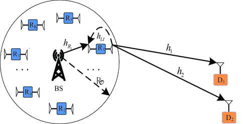
Figure 1: An illustration of RS scheme for downlink FD/HD cooperative NOMA networks.

II-B Signal Model

During the $l$-th time slot, $l=1,2,3,...$, the BS sends the superposed signal $\sqrt{{a_{1}}{P_{s}}}{x_{1}}\left[l\right]+\sqrt{{a_{2}}{P_{s}}}{x_{2}}\left[l\right]$ to the relay on the basis of NOMA principle [8], where ${{x_{1}}}$ and $x_{2}$ are the normalized signal for $D_{1}$ and $D_{2}$, respectively, i.e, $\mathbb{E}\{x_{1}^{2}\}=\mathbb{E}\{x_{2}^{2}\}=1$. ${{a_{1}}}$ and $a_{2}$ are the corresponding power allocation coefficients. Practically speaking, to stipulate better fairness and QoS requirements between the users [40], we assume that ${a_{2}}\geq{a_{1}}$ with $a_{1}+a_{2}=1$. The LI signal exists at the relay due to it works in FD mode. Therefore the observation at the $i$th relay $R_{i}$ is given by

$${y_{{R_{i}}}}= {h_{R_{i}}}(\sqrt{{a_{1}}{P_{s}}}{x_{1}}\left[l\right]+\sqrt{{a_{2}}{P_{s}}}{x_{2}}\left[l\right])$$

$$+{h_{LI}}\sqrt{\varpi{P_{r}}}{x_{LI}}\left[{l-{l_{d}}}\right]+{n_{{R_{i}}}},$$ (1)

where ${h_{R_{i}}}=\frac{{{h_{S{R_{i}}}}}}{{\sqrt{1+d_{S{R_{i}}}^{\alpha}}}}$, ${d_{SR_{i}}}$ is the distance between the BS and $R_{i}$ and $\alpha$ denotes the path loss exponent. $\varpi$ is the switching operation factor, where $\varpi=1$ and $\varpi=0$ denote the relay working in FD mode and HD mode, respectively. According to the practical usage scenarios, we can select the different duplex mode. It is worth noting that in FD mode, it is capable of improving the spectrum efficiency, but will suffer from the LI signals. On the contrary, in HD mode, this situation can be avoided precisely. ${{P_{s}}}$ and ${{P_{r}}}$ denote normalized transmission power (i.e., ${{P_{s}}}={{P_{r}}}=1$) at the BS and $R_{i}$, respectively. ${x_{LI}}[l-{l_{d}}]$ denotes the LI signal with ${\mathop{\mathbb{E}}\nolimits}[|{x_{LI}}{|^{2}}]=1$ and an integer ${l_{d}}$ denotes processing delay at $R_{i}$ with ${l_{d}}\geq 1$. ${n_{{R_{i}}}}$ denotes the Gaussian noise at $R_{i}$.

Based on NOMA protocol, SIC is employed at $R_{i}$ to first decode the signal $x_{2}$ of $D_{2}$ having a higher power allocation factor, since $R_{i}$ has a less interference-infested signal to decode the signal $x_{1}$ of $D_{1}$. Based on this, the received signal-to-interference-plus-noise ratio (SINR) at $R_{i}$ to detect $x_{2}$ and $x_{1}$ are given by

$${\gamma_{{D_{2}}\to{R_{i}}}}=\frac{{\rho{{\left|{{h_{R_{i}}}}\right|}^{2}}{a_{2}}}}{{\rho{{\left|{{h_{R_{i}}}}\right|}^{2}}{a_{1}}+\rho\varpi{{\left|{{h_{LI}}}\right|}^{2}}+1}},$$ (2)

and

$${\gamma_{{D_{1}}\to{R_{i}}}}=\frac{{\rho{{\left|{{h_{R_{i}}}}\right|}^{2}}{a_{1}}}}{{\rho\varpi{{\left|{{h_{LI}}}\right|}^{2}}+1}},$$ (3)

respectively, where $\rho=\frac{{{P_{s}}}}{{{N_{0}}}}$ is the transmit SNR.

Assuming that $R_{i}$ is capable of decoding the two NOMA user’s information, i.e, satisfying the following conditions, 1) $\log\left({1+{\gamma_{{D_{1}}\to{R_{i}}}}}\right)\geq{R_{{D_{1}}}}$; and 2) $\log\left({1+{\gamma_{{D_{2}}\to{R_{i}}}}}\right)\geq{R_{{D_{2}}}}$, where ${R_{{D_{1}}}}$ and ${R_{{D_{2}}}}$ are the target rate for $D_{1}$ and $D_{2}$, respectively. Therefore the observation at $D_{j}$ can be expressed as

$${y_{{D_{j}}}}={h_{j}}(\sqrt{{a_{1}}{P_{r}}}{x_{1}}\left[{l-{l_{d}}}\right]+\sqrt{{a_{2}}{P_{r}}}{x_{2}}\left[{l-{l_{d}}}\right])+{n_{{D_{j}}}},$$ (4)

where ${h_{j}}=\frac{{{h_{{R_{i}}{D_{j}}}}}}{{\sqrt{1+d_{{R_{i}}{D_{j}}}^{\alpha}}}}$, $d_{R_{i}D_{j}}$ is the distance between $R_{i}$ and $D_{j}$ (assuming $d_{R_{i}D_{j}}\gg d_{SR_{i}}$); ${d_{{R_{i}D_{j}}}}=\sqrt{d_{S{R_{i}}}^{2}+d_{j}^{2}-2{d_{S{R_{i}}}}{d_{j}}\cos\left({{\theta_{i}}}\right)}$, $j\in\left({1,2}\right)$. ${\theta_{i}}$ denotes the angle $\angle{D_{j}}S{R_{i}}$; ${n_{{D_{j}}}}$ denotes the Gaussian noise at $D_{j}$.

In similar, assuming that SIC can be also invoked successfully by $D_{1}$ to detect the signal of $D_{2}$ having a higher transmit power, who has less interference. Hence the received SINR at $D_{1}$ to detect $x_{2}$ can be given by

$${\gamma_{{D_{2}}\to{D_{1}}}}=\frac{{\rho{{\left|{{h_{1}}}\right|}^{2}}{a_{2}}}}{{\rho{{\left|{{h_{1}}}\right|}^{2}}{a_{1}}+1}}.$$ (5)

Then the received SINR at $D_{1}$ to detect its own information is given by

$${\gamma_{{D_{1}}}}=\rho{\left|{{h_{1}}}\right|^{2}}{a_{1}}.$$ (6)

The received SINR at $D_{2}$ to detect $x_{2}$ is given by

$${\gamma_{{D_{2}}}}=\frac{{\rho{{\left|{{h_{2}}}\right|}^{2}}{a_{2}}}}{{\rho{{\left|{{h_{2}}}\right|}^{2}}{a_{1}}+1}}.$$ (7)

Note that the fixed power allocation coefficients for two NOMA users are considered in the networks. Reasonable power control and optimizing the mode of power allocation can further enhance the performance of the RS schemes, which may be investigated in our future work.

II-C Relay Selection Schemes

In this subsection, we consider a pair of RS schemes for FD/HD NOMA, which are detailed in the following.

II-C1 Single-stage Relay Selection

Prior to the transmissions, a relay can be randomly selected by the BS as its helper to forward the information. The aim of SRS scheme is to maximize the minimum data rate of $D_{2}$ for FD/HD NOMA. More specifically, the size of data rate for $D_{2}$ depends on three kinds of data rates, such as 1) the data rate for the relay $R_{i}$ to detect $x_{2}$; 2) The data rate for $D_{1}$ to detect $x_{2}$; and 3) the data rate for $D_{2}$ to detect its own signal $x_{2}$. Among the relays in the network, based on (2), (5) and (7), the SRS scheme activates a relay, i.e.,

$${i_{SRS}^{*}}= \mathop{\arg}\limits_{i}\max\left\{{\min\left\{{\log\left({1+{\gamma_{{D_{2}}\to{R_{i}}}}}\right),\log\left({1+{\gamma_{{D_{2}}\to{D_{1}}}}}\right)}\right.}\right.,$$

$$\begin{array}[]{*{20}{c}}{}\hfil&{}\hfil&{}\hfil&{}\hfil&{}\hfil&{}\hfil\\ \end{array}\begin{array}[]{*{20}{c}}{\left.{\left.{\log\left({1+{\gamma_{{D_{2}}}}}\right)}\right\}},i\in S_{R}^{1}\right\}},&{}\hfil\\ \end{array}$$ (10)

where ${S_{R}^{1}}$ denotes the number of relays in the network. Note that FD/HD-based SRS schemes inherit advantage to ensure the data rate of $D_{2}$, where the application of small packets can be achieved.

II-C2 Two-stage Relay Selection

The TRS scheme mainly include two stages for FD/HD NOMA: 1) In the first stage, the target data rate of $D_{2}$ is to be satisfied; and 2) In the second stage, on the condition that the data rate of $D_{2}$ is ensured, we serve $D_{1}$ with data rate as large as possible. Hence the first stage activates the relays that satisfy the following condition

$$S_{R}^{2}= \left\{{\log\left({1+{\gamma_{{D_{2}}\to{R_{i}}}}}\right)\geq{R_{{D_{2}}}},}\right.\log\left({1+{\gamma_{{D_{2}}\to{D_{1}}}}}\right)\geq{R_{{D_{2}}}},$$

$$\begin{array}[]{*{20}{c}}{\left.{\log\left({1+{\gamma_{{D_{2}}}}}\right)\geq{R_{{D_{2}}}},1\leq i\leq K}\right\}},\\ \end{array}$$ (14)

where the size of $S_{R}^{2}$ is defined as $\left|{S_{R}^{2}}\right|$.

Among the relays in $S_{R}^{2}$, the second stage selects a relay to convey the information which can maximize the data rate of $D_{1}$ and is expressed as

$$i_{TRS}^{*}= \mathop{\arg}\limits_{i}\max\left\{{\min\left\{{\log\left({1+{\gamma_{{D_{1}}\to{R_{i}}}}}\right),}\right.}\right.$$

$$\left.{\begin{array}[]{*{20}{c}}{}\hfil&{}\hfil&{}\hfil&{}\hfil&{}\hfil&{}\hfil\\ \end{array}\begin{array}[]{*{20}{c}}{\left.{\log\left({1+{\gamma_{{D_{1}}}}}\right)}\right\},i\in S_{R}^{2}}\\ \end{array}}\right\}.$$ (17)

As can be observed from the above explanations, the merit of FD/HD-based TRS schemes is that in addition to guarantee the data rate of $D_{2}$, the BS can support $D_{1}$ to carry out some background tasks, i.e., downloading a movie or multimedia files.

III Performance evaluation

In this section, the performance of this pair of RS schemes are characterized in terms of outage probability as well as the delay-limited throughput for FD/HD NOMA networks.

III-A Single-stage Relay Selection Scheme

According to NOMA protocol, the complementary events of outage for SRS scheme can be explained as: 1) The relay $i_{SRS}^{*}$ can detect the signal $x_{2}$ of $D_{2}$; and 2) while the signal $x_{2}$ can be successfully detected at $D_{1}$ and $D_{2}$, respectively. From the above descriptions, the outage probability of SRS scheme for FD NOMA can be expressed as follows:

$$P_{SRS}^{FD}=\prod\limits_{i=1}^{K}{\left({1-\Pr\left({{W_{i}}>\gamma_{t{h_{2}}}^{FD}}\right)}\right)},$$ (18)

where ${W_{i}}=\min\left\{{{\gamma_{{D_{2}}\to{R_{i}}}},{\gamma_{{D_{2}}\to{D_{1}}}},{\gamma_{{D_{2}}}}}\right\}$ and $\varpi=1$. $\gamma_{t{h_{2}}}^{FD}=2^{R_{D_{2}}}-1$ with $R_{D_{2}}$ being the target rate of $D_{2}$.

The following theorem provides the outage probability of SRS scheme for FD NOMA.

Theorem 1.

The closed-form expression of outage probability for FD-based NOMA SRS scheme can be approximated as follows:

$$P_{SRS}^{FD}\approx \left[{1-\left({1-\frac{\pi}{{2N}}\sum\limits_{n=1}^{N}{\sqrt{1-\phi_{n}^{2}}}\left({{\phi_{n}}+1}\right)}\right.}\right.$$

$${\left.{\left.{\times\left({1-\frac{{{e^{-{c_{n}}\tau}}}}{{{1+\varpi\rho\tau{c_{n}}{\Omega_{{\rm{LI}}}}}}}}\right)}\right){e^{-\left({1+d_{1}^{\alpha}}\right)\tau-\left({1+d_{2}^{\alpha}}\right)\tau}}}\right]^{K}},$$ (19)

where $\varpi=1$, ${\tau}{\rm{=}}\frac{{\gamma_{t{h_{2}}}^{FD}}}{{\rho\left({{a_{2}}-{a_{1}}\gamma_{t{h_{2}}}^{FD}}\right)}}$ with ${a_{2}}>{a_{1}}\gamma_{t{h_{2}}}^{FD}$. ${c_{n}}=1+{\left({\frac{{{R_{\cal D}}}}{2}\left({{\phi_{n}}+1}\right)}\right)^{\alpha}}$, ${\phi_{n}}=\cos\left({\frac{{2n-1}}{{2N}}\pi}\right)$ and $N$ is a parameter to ensure a complexity-accuracy tradeoff.

Proof.

See Appendix A. ∎

Corollary 1.

Upon substituting $\varpi=0$ into (1), the approximate expression of outage probability for HD-based NOMA SRS scheme is given by

$$P_{SRS}^{HD}\approx \left[{1-\left({1-\frac{\pi}{{2N}}\sum\limits_{n=1}^{N}{\sqrt{1-\phi_{n}^{2}}}\left({{\phi_{n}}+1}\right)}\right.}\right.$$

$${\left.{\left.{\times\left({1-{e^{-{\tau_{1}}{c_{n}}}}}\right)}\right){e^{-\left({1+d_{1}^{\alpha}}\right){\tau_{1}}-\left({1+d_{2}^{\alpha}}\right){\tau_{1}}}}}\right]^{K}},$$ (20)

where ${\tau_{1}}{\rm{=}}\frac{{\gamma_{t{h_{2}}}^{HD}}}{{\rho\left({{a_{2}}-{a_{1}}\gamma_{t{h_{2}}}^{HD}}\right)}}$ with ${a_{2}}>{a_{1}}\gamma_{t{h_{2}}}^{HD}$ and $\gamma_{t{h_{2}}}^{HD}=2^{2{R_{D_{2}}}}-1$ with ${R_{D_{2}}}$ being the target rate of $D_{2}$.

III-B Two-stage Relay Selection Scheme

In the case of TRS scheme, the overall outage event can be expressed [36] as follows:

$$\varphi={\varphi_{1}}\cup{\varphi_{2}},$$ (21)

where ${\varphi_{1}}$ denotes the outage event that relay $i_{TRS}^{*}$ cannot detect $x_{2}$, or neither $D_{1}$ and $D_{2}$ can detect the $x_{2}$ correctively, and ${\varphi_{2}}$ denotes the outage event that either of $i_{TRS}^{*}$ and $D_{1}$ cannot detect $x_{1}$ while three nodes can detect $x_{2}$ successfully.

As a consequence, the outage probability of TRS scheme for FD NOMA can be expressed as follows:

$$P_{TRS}^{FD}=\Pr\left({{\varphi_{1}}}\right)+\Pr\left({{\varphi_{2}}}\right).$$ (22)

On the basis of analytical results in (III-A), the first outage probability in (22) is approximated as

$$\Pr\left({{\varphi_{1}}}\right)\approx \left[{1-\left({1-\frac{\pi}{{2N}}\sum\limits_{n=1}^{N}{\sqrt{1-\phi_{n}^{2}}}\left({{\phi_{n}}+1}\right)}\right.}\right.$$

$${\left.{\left.{\times\left({1-\frac{{{e^{-{c_{n}}{\tau}}}}}{{{1+\rho\varpi\tau{c_{n}}{\Omega_{{\rm{LI}}}}}}}}\right)}\right){e^{-\left({1+d_{1}^{\alpha}}\right){\tau}-\left({1+d_{2}^{\alpha}}\right){\tau}}}}\right]^{K}},$$ (23)

where $\varpi=1$.

In order to calculate the second outage probability, ${\mathop{\rm P}\nolimits}\left({{\varphi_{2}}}\right)$ can be further expressed as

$$\Pr\left({{\varphi_{2}}}\right)=\Pr\left({{\Lambda_{1}},\left|{S_{R}^{2}}\right|>0}\right)+\Pr\left({{\Lambda_{2}},{{\bar{\Lambda}}_{1}},\left|{S_{R}^{2}}\right|>0}\right),$$ (24)

where ${{\Lambda_{1}}}$ denotes the outage event that the relay $i_{TRS}^{*}$ cannot detect $x_{1}$ and ${{{\bar{\Lambda}}_{1}}}$ denotes the corresponding complementary event of ${{\Lambda_{1}}}$. ${{\Lambda_{2}}}$ denotes that $D_{1}$ cannot detect $x_{1}$. The first term in the above equation is given by

$$\Pr\left({{\Lambda_{1}},\left|{S_{R}^{2}}\right|>0}\right)$$ (25)

$$=\Pr\left({\log\left({1+{\gamma_{{D_{1}}\to{R_{i_{TRS}^{*}}}}}}\right)<{R_{{D_{1}}}},\left|{S_{R}^{2}}\right|>0}\right).$$

The second term in (24) is given by

$$\Pr\left({{\Lambda_{2}},{{\bar{\Lambda}}_{1}},\left|{S_{R}^{2}}\right|>0}\right)={\Pr}\left({\log\left({1+{\gamma_{{D_{1}}}}}\right)<{R_{{D_{1}}}},}\right.$$

$$\begin{array}[]{*{20}{c}}{}\hfil&{}\hfil&{}\hfil&{}\hfil&{}\hfil&{}\hfil&{\log\left({1+{\gamma_{{D_{1}}\to{R_{i_{TRS}^{*}}}}}}\right)>{R_{{D_{1}}}}\left.{,\left|{S_{R}^{2}}\right|>0}\right)}.\end{array}$$ (27)

Combining (25) with (III-B), the second outage probability in (22) can be expressed as

$$\Pr\left({{\varphi_{2}}}\right)=\Pr\left({\log\left({1+{\gamma_{{D_{1}}\to{R_{i_{TRS}^{*}}}}}}\right)<{R_{{D_{1}}}},\left|{S_{R}^{2}}\right|>0}\right)$$

$$\begin{array}[]{*{20}{c}}{}\hfil&{}\hfil&{}\hfil&{+\Pr\left({\log\left({1+{\gamma_{{D_{1}}}}}\right)<{R_{{D_{1}}}},}\right.}\\ \end{array}$$

$$\begin{array}[]{*{20}{c}}{}\hfil&{}\hfil&{}\hfil&{\log\left({1+{\gamma_{{D_{1}}\to{R_{i_{TRS}^{*}}}}}}\right)>{R_{{D_{1}}}}\left.{,\left|{S_{R}^{2}}\right|>0}\right)},\end{array}$$ (29)

where $\varpi=1$.

To derive the closed-form expression of outage probability for TRS scheme in (III-B), we define

$${s_{i}}=\min\left\{{\log\left({1+{\gamma_{{D_{1}}\to{R_{i}}}}}\right),\log\left({1+{\gamma_{{D_{1}}}}}\right)}\right\},$$ (30)

and

$${s_{{i_{TRS}^{*}}}}=\max\left\{{{s_{k}},\forall k\in S_{R}^{2}}\right\},$$ (31)

respectively. The probability $\Pr\left({{\varphi_{2}}}\right)$ can be given by

$$\Pr\left({{\varphi_{2}}}\right)= \Pr\left({\min\left\{{\log\left({1+{\gamma_{{D_{1}}\to{R_{i_{TRS}^{*}}}}}}\right),}\right.}\right.$$

$$\left.{\begin{array}[]{*{20}{c}}{}\hfil&{}\hfil&{}\hfil&{\left.{\log\left({1+{\gamma_{{D_{1}}}}}\right)}\right\}}\\ \end{array}<{R_{{D_{1}}}},\left|{S_{R}^{2}}\right|>0}\right)$$

$$= \Pr\left({{s_{{i_{TRS}^{*}}}}<{R_{{D_{1}}}},\left|{S_{R}^{2}}\right|>0}\right).$$ (32)

The above probability can be further expressed as

$$\Pr\left({{\varphi_{2}}}\right)= \sum\limits_{k=1}^{K}{\Pr\left({{s_{{i_{TRS}^{*}}}}<{R_{{D_{1}}}},\left|{S_{R}^{2}}\right|=k}\right)}$$

$$= \sum\limits_{k=1}^{K}{\Pr\left({{s_{i_{TRS}^{*}}}<{R_{{D_{1}}}}|\left|{S_{R}^{2}}\right|=k}\right)\Pr\left({\left|{S_{R}^{2}}\right|=k}\right)}$$

$$= \sum\limits_{k=1}^{K}{{{\left[{\underbrace{F\left({{R_{{D_{1}}}}}\right)}_{{\Theta_{1}}}}\right]}^{k}}\underbrace{\Pr\left({\left|{S_{R}^{2}}\right|=k}\right)}_{{\Theta_{2}}}}.$$ (33)

For selecting a relay at random from ${S_{R}^{2}}$, denoted by relay ${i_{R}}$, let us now turn our attention to the derivation of ${s_{{i_{R}}}}$’s CDF (i.e., ${F\left({{R_{{D_{1}}}}}\right)}$) in the following lemma. Define these two probabilities at the right hand side of (III-B) by ${{\rm{\Theta}}_{1}}$ and ${{\rm{\Theta}}_{2}}$, respectively.

Lemma 1.

The conditional probability in (III-B) can be approximated as follows:

$${{\rm{\Theta}}_{1}}\approx\frac{{{{M}_{1}}+{{M}_{2}}+{{M}_{3}}}}{{{e^{-\left({1+d_{1}^{\alpha}}\right){\tau}}}\left({1-\Delta\left({1-\chi{e^{-{c_{n}}{\tau}}}}\right)}\right)}},$$ (34)

where $\Delta{\rm{=}}\frac{\pi}{{2N}}\sum\limits_{n=1}^{N}{\sqrt{1-\phi_{n}^{2}}}\left({{\phi_{n}}+1}\right)$, $\theta{\rm{=}}\max\left({{\tau},\xi}\right)$, $\xi{\rm{=}}\frac{{\gamma_{t{h_{1}}}^{FD}}}{{\rho{a_{1}}}}$, $\zeta=\frac{{{c_{n}}+\left({1+d_{1}^{\alpha}}\right)}}{{\rho\varpi{c_{n}}}}$, $\chi=\frac{1}{{1+\rho\varpi{\tau}{c_{n}}{\Omega_{{\rm{LI}}}}}}$, $\psi=\frac{1}{{1+\rho\varpi\xi{c_{n}}{\Omega_{{\rm{LI}}}}}}$, ${\rm T}=\frac{{\left({1+d_{1}^{\alpha}}\right){e^{-\left({{c_{n}}+\left({1+d_{1}^{\alpha}}\right)}\right)\xi}}}}{{\rho\varpi{c_{n}}{\Omega_{{\rm{LI}}}}}}$, $\Phi=\frac{{\left({1+d_{1}^{\alpha}}\right){e^{-\left({{c_{n}}+\left({1+d_{1}^{\alpha}}\right)}\right){\tau}}}}}{{\rho\varpi{c_{n}}{\Omega_{{\rm{LI}}}}}}$, ${{M}_{1}}={e^{-\left({1+d_{1}^{\alpha}}\right)\theta}}\Delta\left({\chi{e^{-{c_{n}}{\tau}}}-\psi{e^{-{c_{n}}\xi}}}\right)$, ${{M}_{2}}=\Delta\left({\left({{e^{-\left({1+d_{1}^{\alpha}}\right){\tau}}}-{e^{-\left({1+d_{1}^{\alpha}}\right)\xi}}}\right){e^{-{c_{n}}{\tau}}}\chi-{\rm T}{e^{\frac{\zeta}{{{\Omega_{{\rm{LI}}}}\psi}}}}{{\mathop{\rm E}\nolimits}_{\mathop{\rm i}\nolimits}}\left({\frac{{-\zeta}}{{{\Omega_{{\rm{LI}}}}\psi}}}\right)}\right.\\ \left.{+\Phi{e^{\frac{{-\zeta}}{{{\Omega_{{\rm{LI}}}}\chi}}}}{{\mathop{\rm E}\nolimits}_{\mathop{\rm i}\nolimits}}\left({\frac{{-\zeta}}{{{\Omega_{{\rm{LI}}}}\chi}}}\right)}\right)$, ${M_{3}}={e^{-\left({1+d_{1}^{\alpha}}\right)\tau}}-{e^{-\left({1+d_{1}^{\alpha}}\right)\xi}}-\Delta\left({{e^{-\left({1+d_{1}^{\alpha}}\right)\tau}}-{e^{-\left({1+d_{1}^{\alpha}}\right)\xi}}-{\rm T}{e^{\frac{\zeta}{{{\Omega_{{\rm{LI}}}}\psi}}}}{{\mathop{\rm E}\nolimits}_{\mathop{\rm i}\nolimits}}\left({\frac{{-\zeta}}{{{\Omega_{{\rm{LI}}}}\psi}}}\right)+\Phi{e^{\frac{{-\zeta}}{{{\Omega_{{\rm{LI}}}}\chi}}}}}\right.\\ \left.{\times{{\mathop{\rm E}\nolimits}_{\mathop{\rm i}\nolimits}}\left({\frac{{-\zeta}}{{{\Omega_{{\rm{LI}}}}\chi}}}\right)}\right)$, $\gamma_{t{h_{1}}}^{FD}=2^{R_{D_{1}}}-1$ with $R_{D_{1}}$ being the target rate of $D_{1}$ and ${{\mathop{\rm E}\nolimits}_{\mathop{\rm i}\nolimits}}\left(\cdot\right)$ is the exponential integral function [41, Eq. (8.211.1)].

Proof.

See Appendix B. ∎

On the other hand, there are $k$ relays in ${S_{R}^{2}}$ and the corresponding probability ${{\rm{\Theta}}_{2}}$ is given by

$${{\rm{\Theta}}_{2}}= \prod\limits_{m=1}^{K-k}{K\choose k}{\left({1-\Pr\left({{\gamma_{{D_{2}}\to{R_{i}}}}>\gamma_{t{h_{2}}}^{FD}}\right)}\right.}$$

$$\left.{\times\Pr\left({{\gamma_{{D_{1}}\to{D_{2}}}}>\gamma_{t{h_{2}}}^{FD}}\right)\Pr\left({{\gamma_{{D_{2}}}}>\gamma_{t{h_{2}}}^{FD}}\right)}\right)$$

$$\times\prod\limits_{m=K-k+1}^{K}{\Pr\left({{\gamma_{{D_{2}}\to{R_{i}}}}>\gamma_{t{h_{2}}}^{FD}}\right)}$$

$$\times\Pr\left({{\gamma_{{D_{1}}\to{D_{2}}}}>\gamma_{t{h_{2}}}^{FD}}\right)\Pr\left({{\gamma_{{D_{2}}}}>\gamma_{t{h_{2}}}^{FD}}\right).$$ (35)

With the aid of Theorem 1, the above probability can be further approximated as follows:

$${\Theta_{2}}\approx {K\choose k}\left[{1-\left({1-\frac{\pi}{{2N}}\sum\limits_{n=1}^{N}{\sqrt{1-\phi_{n}^{2}}}}\right.}\right.\left({{\phi_{n}}+1}\right)$$

$$\times\left.{\left({1-\frac{{{e^{-{c_{n}}{\tau}}}}}{{1+\rho\varpi\tau{c_{n}}{\Omega_{{\rm{LI}}}}}}}\right)}\right){\left.{{e^{-\left({1+d_{1}^{\alpha}}\right){\tau}-\left({1+d_{2}^{\alpha}}\right){\tau}}}}\right]^{K-k}}$$

$$\times\left[{\left({1-\frac{\pi}{{2N}}\sum\limits_{n=1}^{N}{\sqrt{1-\phi_{n}^{2}}}}\right.}\right.\left({{\phi_{n}}+1}\right)$$

$$\times\left.{\left({1-\frac{{{e^{-{c_{n}}{\tau}}}}}{{1+\rho\varpi\tau{c_{n}}{\Omega_{{\rm{LI}}}}}}}\right)}\right){\left.{{e^{-\left({1+d_{1}^{\alpha}}\right){\tau}-\left({1+d_{2}^{\alpha}}\right){\tau}}}}\right]^{k}}.$$ (36)

With the aid of Lemma 1, combining (III-B), (III-B), (34) and (III-B) and applying some algebraic manipulations, the outage probability of TRS scheme for FD NOMA can be provided in the following theorem.

Theorem 2.

The closed-form expression of outage probability for the FD-based NOMA TRS scheme is approximated by (2) at the top of next page.

$$P_{TRS}^{FD}\approx \sum\limits_{k=0}^{K}{K\choose k}\left[{\frac{{{e^{-\left({1+d_{1}^{\alpha}}\right)\theta}}\Delta\left({\chi{e^{-{c_{n}}\tau}}-\psi{e^{-{c_{n}}\xi}}}\right)}}{{{e^{-\left({1+d_{1}^{\alpha}}\right){\tau_{1}}}}\left({1-\Delta\left({1-\chi{e^{-{c_{n}}\tau}}}\right)}\right)}}+\frac{{\Delta\left({{e^{-\left({1+d_{1}^{\alpha}}\right)\tau}}-{e^{-\left({1+d_{1}^{\alpha}}\right)\xi}}}\right){e^{-{c_{n}}\tau}}\chi}}{{{e^{-\left({1+d_{1}^{\alpha}}\right)\tau}}\left({1-\Delta\left({1-\chi{e^{-{c_{n}}\tau}}}\right)}\right)}}}\right.$$

$${\left.{\begin{array}[]{*{20}{c}}{}\hfil&{+\frac{{{e^{-\left({1+d_{1}^{\alpha}}\right)\tau}}-{e^{-\left({1+d_{1}^{\alpha}}\right)\xi}}-\Delta\left({{e^{-\left({1+d_{1}^{\alpha}}\right)\tau}}-{e^{-\left({1+d_{1}^{\alpha}}\right)\xi}}}\right)}}{{{e^{-\left({1+d_{1}^{\alpha}}\right)\tau}}\left({1-\Delta\left({1-\chi{e^{-{c_{n}}\tau}}}\right)}\right)}}}\\ \end{array}}\right]^{k}}{\left[{1-\left({1-\Delta\left({1-\chi{e^{-{c_{n}}\tau}}}\right)}\right){e^{-\left({1+d_{1}^{\alpha}}\right)\tau-\left({1+d_{2}^{\alpha}}\right)\tau}}}\right]^{K-k}}$$ (38)

$$\begin{array}[]{*{20}{c}}{}\hfil&{\times{{\left[{\left({1-\Delta\left({1-\chi{e^{-{c_{n}}\tau}}}\right)}\right){e^{-\left({1+d_{1}^{\alpha}}\right)\tau-\left({1+d_{2}^{\alpha}}\right)\tau}}}\right]}^{k}}}\end{array}.$$ (40)

Corollary 2.

For the special case $\varpi=0$, the approximate expression of outage probability for HD-based NOMA TRS scheme is given by (2) at the top of next page,

$$P_{TRS}^{HD}\approx \sum\limits_{k=0}^{K}{{K\choose k}\left[{\frac{{\Delta\frac{{{c_{n}}}}{{\left({1+d_{1}^{\alpha}}\right)+{c_{n}}}}\left({{e^{-\left({\left({1+d_{1}^{\alpha}}\right)+{c_{n}}}\right){\tau_{1}}}}-{e^{-\left({\left({1+d_{1}^{\alpha}}\right)+{c_{n}}}\right){\xi_{1}}}}}\right)}}{{{e^{-\left({1+d_{1}^{\alpha}}\right){\tau_{1}}}}\left({1-\Delta\left({1-{e^{-{\tau_{1}}{c_{n}}}}}\right)}\right)}}}\right.}$$

$${\left.{+\frac{{{e^{-\left({1+d_{1}^{\alpha}}\right){\tau_{1}}}}-{e^{-\left({1+d_{1}^{\alpha}}\right){\xi_{1}}}}-\Delta\left[{{e^{-\left({1+d_{1}^{\alpha}}\right){\tau_{1}}}}-{e^{-\left({1+d_{1}^{\alpha}}\right){\xi_{1}}}}+\frac{{1+d_{1}^{\alpha}}}{{1+d_{1}^{\alpha}+{c_{n}}}}\left({{e^{-\left({1+d_{1}^{\alpha}+{c_{n}}}\right){\xi_{1}}}}-{e^{-\left({1+d_{1}^{\alpha}+{c_{n}}}\right){\tau_{1}}}}}\right)}\right]}}{{{e^{-\left({1+d_{1}^{\alpha}}\right){\tau_{1}}}}\left({1-\Delta\left({1-{e^{-{\tau_{1}}{c_{n}}}}}\right)}\right)}}}\right]^{k}}$$

$$\times{\left[{1-\left({1-\Delta\left({1-{e^{-{\tau_{1}}{c_{n}}}}}\right)}\right){e^{-\left[{\left({1+d_{1}^{\alpha}}\right)+\left({1+d_{2}^{\alpha}}\right)}\right]{\tau_{1}}}}}\right]^{K-k}}{\left[{\left({1-\Delta\left({1-{e^{-{\tau_{1}}{c_{n}}}}}\right)}\right){e^{-\left[{\left({1+d_{1}^{\alpha}}\right)+\left({1+d_{2}^{\alpha}}\right)}\right]{\tau_{1}}}}}\right]^{k}}.$$ (41)

where $\xi_{1}{\rm{=}}\frac{{\gamma_{t{h_{1}}}^{HD}}}{{\rho{a_{1}}}}$ and $\gamma_{t{h_{1}}}^{HD}=2^{2{R_{D_{1}}}}-1$ with ${R_{D_{1}}}$ being the target rate of $D_{1}$.

III-C Benchmarks for SRS and TRS schemes

In this subsection, we consider the random relay selection (RRS) scheme as a benchmark for comparison purposes, where the relay $R_{i}$ is selected randomly to help the BS transmitting the information. Note that $R_{i}$ selected maybe not the optimal one for the NOMA RS schemes. In this case, the RRS scheme is capable of being regarded as the special case for SRS/TRS schemes with $K=1$, which is independent of the number of relays. As such, for SRS scheme, the outage probability of the RRS scheme for FD/HD NOMA can be easily approximated as

$$P_{RRS}^{FD,SRS}\approx 1-\left[{1-\frac{\pi}{{2N}}\sum\limits_{n=1}^{N}{\sqrt{1-\phi_{n}^{2}}}\left({{\phi_{n}}+1}\right)}\right.$$

$$\left.{\times\left({1-\frac{{{e^{-{c_{n}}\tau}}}}{{1+\rho\tau{c_{n}}{\Omega_{{\rm{LI}}}}}}}\right)}\right]{e^{-\left({1+d_{1}^{\alpha}}\right)\tau-\left({1+d_{2}^{\alpha}}\right)\tau}},$$ (42)

and

$$P_{RRS}^{HD,SRS}\approx 1-\left[{1-\frac{\pi}{{2N}}\sum\limits_{n=1}^{N}{\sqrt{1-\phi_{n}^{2}}}\left({{\phi_{n}}+1}\right)}\right.$$

$$\left.{\times\left({1-{e^{-{\tau_{1}}{c_{n}}}}}\right)}\right]{e^{-\left({1+d_{1}^{\alpha}}\right){\tau_{1}}-\left({1+d_{2}^{\alpha}}\right){\tau_{1}}}},$$ (43)

respectively. Similarly, for TRS scheme, the outage probability of RRS scheme for FD/HD NOMA can be obtained from (2) and (2) by setting $K=1$, respectively.

III-D Diversity Order Analysis

To gain more insights for these two RS schemes, the asymptotic diversity analysis is provided in the high SNR region according to the derived outage probabilities. The diversity order is defined as

$$d=-\mathop{\lim}\limits_{\rho\to\infty}\frac{{\log\left({P^{\infty}\left(\rho\right)}\right)}}{{\log\rho}},$$ (44)

where ${P^{\infty}\left(\rho\right)}$ is the asymptotic outage probability.

III-D1 Single-stage Relay Selection Scheme

Based on the analytical results in (1), when $\rho\to\infty$, we can derive the asymptotic outage probability of SRS scheme for FD NOMA in the following corollary.

Corollary 3.

The asymptotic outage probability of FD-based NOMA SRS scheme at high SNR is given by

$$P_{SRS}^{FD,\infty}={\left[{\frac{\pi}{{2N}}\sum\limits_{n=1}^{N}{\sqrt{1-\phi_{n}^{2}}}\left({{\phi_{n}}+1}\right)\left({\frac{{\rho\tau{c_{n}}{\Omega_{{\rm{LI}}}}}}{{1+\rho\tau{c_{n}}{\Omega_{{\rm{LI}}}}}}}\right)}\right]^{K}}.$$ (45)

Substituting (45) into (44), we can obtain $d_{SRS}^{FD}=0$.

Remark 1.

The diversity order of SRS scheme for FD NOMA is zero, which is the same as the conventional FD RS scheme.

Corollary 4.

For the special case $\varpi=0$, the asymptotic outage probability of HD-based NOMA SRS scheme with ${e^{-x}}\approx 1-x$ at high SNR is given by

$$P_{SRS}^{HD,\infty}= \left[{1-\left({1-\frac{\pi}{{2N}}\sum\limits_{n=1}^{N}{\sqrt{1-\phi_{n}^{2}}}\left({{\phi_{n}}+1}\right){\tau_{1}}{c_{n}}}\right)}\right.$$

$${\left.{\times\left({1-\left({1+d_{1}^{\alpha}+1+d_{2}^{\alpha}}\right){\tau_{1}}}\right)}\right]^{K}}.$$ (46)

Substituting (4) into (44), we can obtain $d_{SRS}^{HD}=K$.

Remark 2.

The diversity order of SRS scheme for HD NOMA is $K$, which provides a diversity order equal to the number of the available relays.

III-D2 Two-stage Relay Selection Scheme

As such, we can derive asymptotic outage probability of TRS scheme for FD NOMA in the following corollary.

Corollary 5.

The asymptotic outage probability of FD-based NOMA TRS scheme at high SNR is given by

$$P_{TRS}^{FD,\infty}= {\sum\limits_{k=0}^{K}{{K\choose k}\left[{\frac{{\Delta\left({2\chi-\psi}\right)}}{{1-\Delta\left({1-\chi}\right)}}}\right]}^{k}}{\left[{\Delta\left({1-\chi}\right)}\right]^{K-k}}$$

$$\times{\left[{\left({1-\Delta\left({1-\chi}\right)}\right)}\right]^{k}}.$$ (47)

Proof.

See Appendix C. ∎

Upon substituting (5) into (44), we obtain $d_{TRS}^{FD}=0$.

Remark 3.

The zero diversity order of TRS scheme for FD NOMA is obtained, which is the same as the FD-based SRS scheme.

Corollary 6.

For the special case $\varpi=0$, the asymptotic outage probability of HD-based NOMA TRS scheme with ${e^{-x}}\approx 1-x$ at high SNR is given by

$$P_{TSR}^{HD,\infty}= \sum\limits_{k=0}^{K}{{K\choose k}\left[{\frac{{\Delta{c_{n}}\left[{{\xi_{1}}-{\tau_{1}}}\right]{\rm{+}}\left({1+d_{1}^{\alpha}}\right){\xi_{1}}}}{{1-\Delta{\tau_{1}}{c_{n}}}}}\right.}$$

$$-\frac{{\left({1+d_{1}^{\alpha}}\right){\tau_{1}}+\Delta\left[{\left({1+d_{1}^{\alpha}}\right){\xi_{1}}-\left({1+d_{1}^{\alpha}}\right){\tau_{1}}}\right]}}{{1-\Delta{\tau_{1}}{c_{n}}}}$$

$${\left.{-\frac{{\Delta\left({1+d_{1}^{\alpha}}\right)\left({{\tau_{1}}-{\xi_{1}}}\right)}}{{1-\Delta{\tau_{1}}{c_{n}}}}}\right]^{k}}{\left({\Delta{\tau_{1}}{c_{n}}}\right)^{K-k}}{\left({1-\Delta{\tau_{1}}{c_{n}}}\right)^{k}}.$$ (48)

Upon substituting (6) into (44), we obtain $d_{TRS}^{HD}=K$.

Remark 4.

The diversity order of TRS scheme for HD cooperative NOMA is K, which is the same as the HD-based SRS scheme.

III-D3 Random Relay Selection Scheme

For SRS scheme, based on the analytical results in (45) and (4), the asymptotic outage probability of RRS scheme for FD/HD NOMA with $K=1$ can be given by

$$P_{RRS,SRS}^{FD,\infty}=\frac{\pi}{{2N}}\sum\limits_{n=1}^{N}{\sqrt{1-\phi_{n}^{2}}}\left({{\phi_{n}}+1}\right)\left({\frac{{{c_{n}}\rho\tau{\Omega_{{\rm{LI}}}}}}{{1+{c_{n}}\rho\tau{\Omega_{{\rm{LI}}}}}}}\right),$$ (49)

and

$$P_{RRS,SRS}^{HD,\infty}= {1-\left({1-\frac{\pi}{{2N}}\sum\limits_{n=1}^{N}{\sqrt{1-\phi_{n}^{2}}}\left({{\phi_{n}}+1}\right){\tau_{1}}{c_{n}}}\right)}$$

$${{\times\left({1-\left({1+d_{1}^{\alpha}+1+d_{2}^{\alpha}}\right){\tau_{1}}}\right)}},$$ (50)

respectively.

For TRS scheme, based on the analytical results in (5) and (6), the asymptotic outage probability of RRS scheme for FD/HD NOMA with $K=1$ can be given by

$$P_{RRS,TRS}^{FD,\infty}= {\sum\limits_{k=0}^{1}{{1\choose k}\left[{\frac{{\Delta\left({2\chi-\psi}\right)}}{{1-\Delta\left({1-\chi}\right)}}}\right]}^{k}}{\left[{\Delta\left({1-\chi}\right)}\right]^{1-k}}$$

$$\times{\left[{\left({1-\Delta\left({1-\chi}\right)}\right)}\right]^{k}},$$ (51)

and

$$P_{RRS,TSR}^{HD,\infty}= \sum\limits_{k=0}^{1}{{1\choose k}\left[{\frac{{\Delta{c_{n}}\left[{{\xi_{1}}-{\tau_{1}}}\right]{\rm{+}}\left({1+d_{1}^{\alpha}}\right){\xi_{1}}}}{{1-\Delta{\tau_{1}}{c_{n}}}}}\right.}$$

$$-\frac{{\left({1+d_{1}^{\alpha}}\right){\tau_{1}}+\Delta\left[{\left({1+d_{1}^{\alpha}}\right){\xi_{1}}-\left({1+d_{1}^{\alpha}}\right){\tau_{1}}}\right]}}{{1-\Delta{\tau_{1}}{c_{n}}}}$$

$${\left.{-\frac{{\Delta\left({1+d_{1}^{\alpha}}\right)\left({{\tau_{1}}-\xi}\right)}}{{1-\Delta{\tau_{1}}{c_{n}}}}}\right]^{k}}{\left({\Delta{\tau_{1}}{c_{n}}}\right)^{1-k}}$$

$$\times{\left({1-\Delta{\tau_{1}}{c_{n}}}\right)^{k}},$$ (52)

respectively.

Remark 5.

Substituting (49), (III-D3) and (III-D3), (III-D3) into (44), we can observed that the diversity orders of RRS scheme for FD-NOMA and HD-NOMA are zero and one, respectively.

In order to get intuitional insights, as shown in TABLE I, the diversity orders and application scenarios of FD/HD-based NOMA RS schemes are summarized to illustrate the comparison between them. For the sake of simplicity, we use “D” to represent the diversity order.

Duplex mode	RS scheme	D	Application scenario
FD NOMA	SRS	0	Small packet service
	TRS	0	Background tasks
	RRS	0	——
HD NOMA	SRS	K	Small packet service
	TRS	K	Background tasks
	RRS	1	——

TABLE I: Diversity orders and application scenarios for FD/HD-based NOMA RS schemes.

III-E Throughput Analysis

In this subsection, the delay-limited transmission modes of these RS schemes are investigated for FD/HD NOMA networks. In this mode, the BS sends information at a constant rate and the system throughput is subjective to the effect of outage probability. Hence it is significant to discuss the system throughput for delay-limited mode in practical scenarios.

Proposition 1.

Based on above explanation, the system throughput of the RS schemes for FD/HD NOMA are given by

$$R_{\Psi}^{FD}=\left({1-P_{\Psi}^{FD}}\right){R_{{D_{1}}}}+\left({1-P_{\Psi}^{FD}}\right){R_{{D_{2}}}},$$ (53)

and

$$R_{\Psi}^{HD}=\left({1-P_{\Psi}^{HD}}\right){R_{{D_{1}}}}+\left({1-P_{\Psi}^{HD}}\right){R_{{D_{2}}}},$$ (54)

respectively, where $\Psi\in\left\{{SRS,TRS}\right\}$. ${R_{SRS}}$ and ${R_{TRS}}$ are system throughputs of single-stage and two-stage RS schemes, respectively.

IV Numerical Results

In this section, our numerical results are provided for characterizing the outage performance of these two kinds of RS schemes. Monte Carlo simulation parameters used in this section are summarized in Table II [42, 12], in which BPCU is short for bit per channel use. The complexity-vs-accuracy tradeoff parameter is $N=15$. Except FD/HD-based NOMA RRS schemes, the performance of OMA-based RS scheme is also shown as a benchmark for comparison, where the total communication process is finished in four slots. In the first slot, the BS sends information $x_{1}$ to relay $R_{i}$ and send $x_{2}$ to $R_{i}$ in the second slot. In the third and fourth slot, $R_{i}$ decodes and forwards the information $x_{1}$ and $x_{2}$ to $D_{1}$ and $D_{2}$, respectively. Adding the performance of AF-based RS schemes for comparison will further enrich this paper, but this is beyond the scope of this paper. Note that NOMA users with low target data rate can be applied to the IoT scenarios, i.e., the low energy consumption, small packet service and so on.

Monte Carlo simulations repeated	${10^{6}}$ iterations
Power allocation coefficients of NOMA	$a_{1}=0.2$, $a_{2}=0.8$
Targeted data rates	$R_{D_{1}}=1$, $R_{D_{2}}=0.1$ BPCU
Pass loss exponent	$\alpha=2$
The radius of a disc region	${R_{\cal D}}=2$ m
The distance between the BS and $D_{1}$	$10$ m
The distance between the BS and $D_{2}$	$12$ m

TABLE II: Table of Parameters for numerical results.

IV-A Single-stage Relay Selection Scheme

In this subsection, the FD/HD-based NOMA RRS schemes and OMA-based RS schemes are regarded as the baselines for comparison purposes.

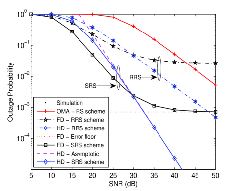
Figure 2: Outage probability versus the transmit SNR for SRS scheme with $K=2$; ${R_{D_{1}}}=1$, ${R_{D_{2}}}=0.1$ BPCU and $\mathbb{E}\{|h_{LI}|^{2}\}=-10$ dB.

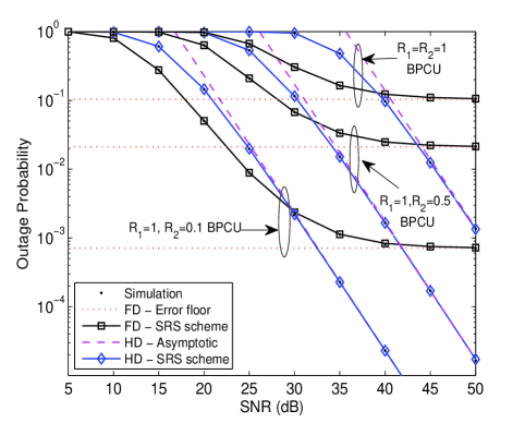
Figure 3: Outage probability versus the transmit SNR for SRS scheme with the different target rates; $K=2$ and $\mathbb{E}\{|h_{LI}|^{2}\}=-10$ dB.

Fig. 2 plots the outage probability of SRS scheme versus SNR for a simulation setting with $K=2$ and $\mathbb{E}\{|h_{LI}|^{2}\}=-10$ dB. The black and blue solid curves are the SRS scheme for FD/HD NOMA, corresponding to the approximate results derived in (1) and (1), respectively. The dash dotted curves represent the approximate outage probabilities of RRS schemes for FD/HD NOMA derived in (III-C) and (III-C), respectively. Obviously, the outage probability curves match precisely with the Monte Carlo simulation results. It is observed that the performance of FD-based NOMA SRS scheme is superior to HD-based NOMA scheme on the condition of low SNR region. The reason is that loop interference is not the dominant impact factor for FD cooperative NOMA in the low SNR region. Moreover, the outage performance of the HD-based NOMA SRS scheme outperforms the HD-based RRS scheme. Another observation is that HD-based NOMA SRS scheme is superior to OMA-based RS scheme. This is due to the fact that HD-based NOMA RS schemes is capable of enhancing the spectral efficiency compared to OMA. The asymptotic outage probability cures of the SRS schemes for FD/HD NOMA are plotted according to the analytical results in (45) and (4), respectively. One can observe that the asymptotic curves well approximate the analytical performance curves in the high SNR region. It is worth noting that an error floor exists in the FD-based NOMA SRS scheme, which verifies the conclusion in Remark 1 and obtain zero diversity order. This is due to the fact that there is the loop interference in FD NOMA.

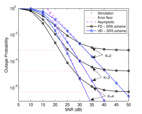
Figure 4: Outage probability versus the transmit SNR for SRS scheme with $K=2,3,4$; ${R_{D_{1}}}=1$, ${R_{D_{2}}}=0.1$ BPCU and $\mathbb{E}\{|h_{LI}|^{2}\}=-10$ dB.

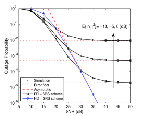
Figure 5: Outage probability versus the transmit SNR for SRS scheme with $K=3$; ${R_{D_{1}}}=1$, ${R_{D_{2}}}=0.1$ BPCU.

Fig. 3 plots the outage probability of SRS scheme with different target rates. One can observe that adjusting the target rates of NOMA users will affect the outage behaviors of the FD/HD-based SRS schemes. As the value of target rates increases, the superior of FD/HD-based NOMA SRS schemes becomes not obvious. It is worth noting that based on the application requirements of different scenarios, the setting of reasonable target rates for NOMA users is prerequisite.

Fig. 4 plots the outage probability of SRS scheme versus SNR for a simulation setting with $K=2,3,4$ relays and $\mathbb{E}\{|h_{LI}|^{2}\}=-10$ dB. As can be seen that the analytical curves perfectly match with the simulation results, while the approximations match the analytical performance curves in the high SNR region. It is shown that the number of relays in the networks considered strongly affect the performance of FD/HD-based NOMA SRS schemes. With the number of relays increasing, the lower outage probability are achieved by this RS scheme. This is because more relays bring higher diversity gains, which improves the reliability of the cooperative networks. Another observation is that the HD-based NOMA SRS scheme provides a diversity order that is equal to the number of the relays ($K$), which verifies the conclusion in Remark 2. As a further development, Fig. 5 plots the outage probability of SRS scheme versus different values of LI from $\mathbb{E}\{|h_{LI}|^{2}\}=-10$ dB to $\mathbb{E}\{|h_{LI}|^{2}\}=5$ dB. As observed from the figure, we can see that the value of LI also strongly affect the performance of FD-based SRS scheme for NOMA, while the HD-based SRS scheme is not affected. This is due to the fact that LI is not existent for the HD-based SRS scheme with $\varpi=0$. As the value of LI becomes larger, the outage performance of the FD-based SRS scheme becomes more worse. In consequence, it is significant to consider the influence of LI in the practical FD NOMA networks.

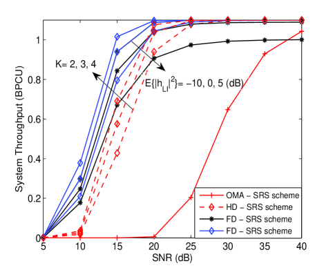
Figure 6: System throughput in delay-limited transmission mode versus SNR for the SRS scheme.

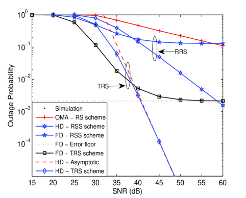
Figure 7: Outage probability versus the transmit SNR for TRS scheme with $K=3$; ${R_{D_{1}}}=1$, ${R_{D_{2}}}=0.1$ BPCU and $\mathbb{E}\{|h_{LI}|^{2}\}=-20$ dB.

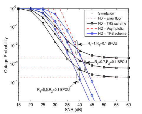
Figure 8: Outage probability versus the transmit SNR for TRS scheme with different target rates; $K=3$ and $\mathbb{E}\{|h_{LI}|^{2}\}=-20$ dB.

Fig. 6 plots system throughput versus SNR in delay-limited transmission mode for the different number of relays from $K=2$ to $K=4$ with $\mathbb{E}\{|h_{LI}|^{2}\}=-10$ dB. The blue solid and red dashed curves represent throughput of SRS scheme for FD/HD NOMA networks which are obtained from (53) and (54), respectively. One can observe that the FD-based SRS scheme achieves a higher throughput compared to the HD-based SRS scheme for NOMA networks. This is because that the value of LI has a smaller influence for the outage behavior of FD NOMA in the low SNR region. Furthermore, the FD/HD-based NOMA SRS schemes outperform OMA-based RS scheme in terms of system throughput. This is due to the fact that NOMA-based SRS scheme can provide more spectrum efficiency than OMA-based SRS scheme. As the number of relays becomes larger, the FD/HD-based SRS schemes can improve the system throughput. This phenomenon can be explained as that a lower outage probability can be obtained by the FD/HD-based SRS schemes. In addition, Fig. 6 further give system throughput in delay-limited transmission mode for the different values of LI with $K=3$. As can be observed that increasing the values of LI from $\mathbb{E}\{|h_{LI}|^{2}\}=-10$ dB to $\mathbb{E}\{|h_{LI}|^{2}\}=5$ dB reduces the system throughput. This phenomenon indicates that it is of significance to consider the impact of LI for FD-based SRS scheme when designing practical cooperative NOMA systems.

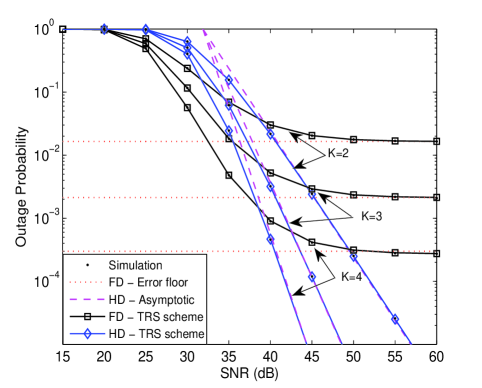
Figure 9: Outage probability versus the transmit SNR for TRS scheme with $K=2,3,4$; ${R_{D_{1}}}=1$, ${R_{D_{2}}}=0.1$ BPCU and $\mathbb{E}\{|h_{LI}|^{2}\}=-20$ dB.

IV-B Two-stage Relay Selection Scheme

In this subsection, except FD/HD-based NOMA RRS scheme, the outage performance of OMA-based RS scheme is also shown as a benchmark for comparison.

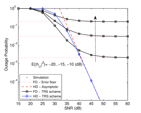
Figure 10: Outage probability versus the transmit SNR for TRS scheme with $K=3$; ${R_{D_{1}}}=1$, ${R_{D_{2}}}=0.1$ BPCU.

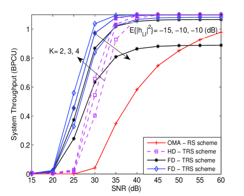
Figure 11: System throughput in delay-limited transmission mode versus SNR for the TRS scheme with ${R_{D_{1}}}=1$, ${R_{D_{2}}}=0.1$ BPCU.

Fig. 7 plots the outage probability of TRS scheme versus SNR with setting to be $K=3$ and $\mathbb{E}\{|h_{LI}|^{2}\}=-20$ dB. The approximate analytical curves of the TRS schemes for FD/HD NOMA are plotted based on (2) and (2), respectively. As can be observed from the figure, the analytical curves match perfectly with Monte Carlo simulation results. We confirm that the higher outage performance can be obtained by FD-based NOMA TRS scheme in the low SNR region. This is due to fact that there is a low loop interference for FD-based TRS scheme and does not suffer from bandwidth-loss influence. One can observe that the outage behaviors of FD/HD-based NOMA TRS schemes outperform OMA-based RS scheme. The asymptotic outage probability curves of FD/HD-based NOMA TRS scheme are plotted according to (5) and (6), which are practically indistinguishable from the analytical results. It is also observed that the FD-based TRS scheme for NOMA converges to an error floor and obtains the zero diversity, which is due to the fact that the loop interference exists at the relay. This phenomenon is confirmed by the insights in Remark 3. However, the HD-based TRS scheme for NOMA overcomes the problem of zero diversity inherent to FD-based scheme.

As shown in Fig. 3, Fig. 8 plots the outage probability of TRS scheme with different target rates. It is shown that when the target rates of NOMA users is reduced, the FD/HD-based NOMA TRS schemes is capable of providing better outage performance. We confirm that the IoT scenarios (i.e., small packet service) considered can be supported by the NOMA-based RS schemes.

Fig. 9 plots the outage probability of TRS scheme versus SNR for a simulation setting to be $K=2,3,4$ relays and $\mathbb{E}\{|h_{LI}|^{2}\}=-20$ dB. We observed that the number of relays affect the performance of TRS scheme. With the number of relays increasing, the superiority of FD/HD-based NOMA TRS schemes is apparent and the lower outage probabilities are obtained. We also see that the HD-based RS scheme is capable of achieving a diversity order of $K$, which confirms the insights in Remark 4. From a practical perspective, it is important to consider multiple relays in the networks when designing the NOMA RS systems. Fig. 10 plots the outage probability of the TRS scheme versus different values of LI from $\mathbb{E}\{|h_{LI}|^{2}\}=-20$ dB to $\mathbb{E}\{|h_{LI}|^{2}\}=-10$ dB. We also can observe that with the value of LI increasing, the superior of outage performance for the FD-based TRS scheme is not existent.

Fig. 11 plots system throughput versus SNR in delay-limited transmission mode for the different number of relays from $K=2$ to $K=4$ with $\mathbb{E}\{|h_{LI}|^{2}\}=-20$ dB. The solid black and dashed magenta curves represent throughput of TRS for FD/HD NOMA networks which are obtained from (53) and (54), respectively. We can also observe that FD-based NOMA TRS scheme has a higher throughput than HD-based scheme in the low SNR region. The reason is that the FD-based TRS scheme is capable of achieving a lower outage probability compared to HD-based scheme. Moreover, the throughput of FD/HD-NOMA TRS schemes precedes that of OMA-based RS scheme. Additionally, it is worth pointing out that adjusting the size of target data rate (i.e., $R_{D_{1}}$ and $R_{D_{2}}$) will affect the system throughput for delay-limited transmission mode. The main performance of TRS scheme trends follow those in Fig. 6. Additionally, as can be seen from the figure that increasing the values of LI from $\mathbb{E}\{|h_{LI}|^{2}\}=-20$ dB to $\mathbb{E}\{|h_{LI}|^{2}\}=-10$ dB reduces the system throughput and the existence of the throughput ceilings in the high SNR region. This is due to the fact that the FD-based TRS scheme converges to the error floor.

V Conclusions

This paper has investigated a pair of RS schemes for FD/HD NOMA networks insightfully. Stochastic geometry has been employed for modeling the locations of relays in the network. New analytical expressions of outage probability for two RS schemes have been derived. Due to the influence of LI at relay, a zero diversity order has been obtained by these two RS schemes for FD NOMA. Based on the analytical results, it was demonstrated that the diversity orders of HD-based RS schemes were determined by the number of relays in the networks considered. Simulation results showed that the FD/HD-based NOMA SRS/TRS schemes are capable of providing better outage behaviors than RRS and OMA-based RS schemes. The system throughput of delay-limited transmission mode for FD/HD-based NOMA RS schemes were discussed. The setting of perfect SIC operation my bring about overestimated performance for the RS schemes considered, hence our future treaties will consider the impact of imperfect SIC. Another promising future research direction is to optimize the power allocation between NOMA users, which can further enhance the performance of NOMA-based RS schemes.

Appendix A: Proof of Theorem 1

Let ${W_{i}}=\min\left\{{{\gamma_{{D_{2}}\to{R_{i}}}},{\gamma_{{D_{2}}\to{D_{1}}}},{\gamma_{{D_{2}}}}}\right\}$, $W=\max\left\{{{W_{1}},{W_{2}}...,{W_{N}}}\right\}$, then

$$\Pr\left({W<\gamma_{t{h_{2}}}^{FD}}\right)= \Pr\left({\max\left\{{{W_{1}},{W_{2}},...,{W_{N}}}\right\}<\gamma_{t{h_{2}}}^{FD}}\right)$$

$$= \prod\limits_{i=1}^{K}{\Pr\left({{W_{i}}<{\gamma_{t{h_{2}}}^{FD}}}\right)}.$$ (A.1)

Hence the outage probability of the FD-based SRS scheme only requires ${\Pr\left({{W_{i}}<\gamma_{t{h_{2}}}^{FD}}\right)}$, which is given by

$$\Pr\left({{W_{i}}<\gamma_{t{h_{2}}}^{FD}}\right)= \Pr\left({\min\left\{{{\gamma_{{D_{2}}\to{R_{i}}}},{\gamma_{{D_{2}}\to{D_{1}}}},{\gamma_{{D_{2}}}}}\right\}<\gamma_{t{h_{2}}}^{FD}}\right)$$

$$= 1-\underbrace{\Pr\left({{\gamma_{{D_{2}}\to{R_{i}}}}>\gamma_{t{h_{2}}}^{FD}}\right)}_{{J_{11}}}$$

$$\times\underbrace{\Pr\left({{\gamma_{{D_{2}}\to{D_{1}}}}>\gamma_{t{h_{2}}}^{FD}}\right)}_{J_{12}}\underbrace{\Pr\left({{\gamma_{{D_{2}}}}>\gamma_{t{h_{2}}}^{FD}}\right)}_{{{J_{13}}}},$$ (A.2)

where $\varpi=1$.

Define ${X_{i}}{\rm{=}}\frac{{{{\left|{{h_{S{R_{i}}}}}\right|}^{2}}}}{{1+d_{S{R_{i}}}^{\alpha}}}$, ${Y_{1i}}{\rm{=}}\frac{{{{\left|{{h_{{R_{i}}{D_{1}}}}}\right|}^{2}}}}{{1+d_{{R_{i}D_{1}}}^{\alpha}}}$, ${Y_{2i}}{\rm{=}}\frac{{{{\left|{{h_{{R_{i}}{D_{2}}}}}\right|}^{2}}}}{{1+d_{{R_{i}D_{2}}}^{\alpha}}}$, and ${Z}={\left|{{h_{LI}}}\right|^{2}}$. As stated in [8, 20] and by utilizing the polar coordinate, the CDF ${F_{{X_{i}}}}$ of $X_{i}$ is given by

$${F_{{X_{i}}}}\left(x\right)=\frac{2}{{R_{\cal D}^{2}}}\int_{0}^{{R_{\cal D}}}{\left({1-{e^{-\left({1+{r^{\alpha}}}\right)x}}}\right)}rdr.$$ (A.3)

However, for many communication scenarios $\alpha>2$, (A.3) does not have a closed-form solution. In this case, the approximate expression of (A.3) can be obtained by using Gaussian-Chebyshev quadrature [43] and given by

$${F_{{X_{i}}}}\left(x\right)\approx\frac{\pi}{{2N}}\sum\limits_{n=1}^{N}{\sqrt{1-\phi_{n}^{2}}}\left({1-{e^{-{c_{n}}x}}}\right)\left({{\phi_{n}}+1}\right).$$ (A.4)

Substituting (2) into (Appendix A: Proof of Theorem 1) and applying algebraic manipulations, ${J_{11}}$ can be further expressed as follows:

$${J_{11}}= 1-\Pr\left({{X_{i}}<\left({\rho\varpi{f_{Z}}\left(z\right)+1}\right){\tau}}\right),$$ (A.5)

where ${f_{Z}}\left(z\right)=\frac{1}{{{\Omega_{LI}}}}{e^{-\frac{z}{{{\Omega_{LI}}}}}}$. By the virtue of approximate expression of CDF for ${X_{i}}$ in (A.4), ${J_{11}}$ is calculated as

$${J_{11}}= {\rm{1}}-\int_{0}^{\infty}{\frac{1}{{{\Omega_{{\rm{LI}}}}}}{e^{-\frac{z}{{{\Omega_{{\rm{LI}}}}}}}}}{F_{{X_{i}}}}\left({\left({\rho\varpi z+1}\right){\tau}}\right)dz$$

$$\approx 1-\frac{\pi}{{2N}}\sum\limits_{n=1}^{N}{\sqrt{1-\phi_{n}^{2}}}\left({{\phi_{n}}+1}\right)\left({1-\frac{{{e^{-{c_{n}}{\tau}}}}}{{{1+\varpi\rho\tau{c_{n}}{\Omega_{{\rm{LI}}}}}}}}\right).$$ (A.6)

On the condition of ${d_{{R_{i}D_{j}}}}=\sqrt{d_{S{R_{i}}}^{2}+d_{j}^{2}-2{d_{j}}{d_{S{R_{i}}}}\cos\left({{\theta_{i}}}\right)}$ and ${d_{{R_{i}D_{j}}}}\gg d_{SR_{i}}$, $j\in\left({1,2}\right)$, to further simplify computational complexity, we assume that the distance between $R_{i}$ and ${D_{j}}$ can be approximated as the distance between the BS and $D_{j}$, i.e., ${d_{{R_{i}D_{j}}}}\approx d_{j}$. It is worth noting through this approximation, the distance $d_{j}$ between the BS and $D_{j}$ is a fixed value. Hence we can obtain the corresponding approximate CDF of ${F_{{Y_{ji}}}}$ i.e., ${F_{{Y_{ji}}}}=1-{e^{-\left({1+d_{j}^{\alpha}}\right)\tau}}$. Upon substituting (5) and (7) into (Appendix A: Proof of Theorem 1), ${J_{12}}$ and ${J_{13}}$ are approximated by

$${J_{12}}=\Pr\left({{Y_{1i}}>{\tau}}\right)\approx{e^{-\left({1+d_{1}^{\alpha}}\right){\tau}}},$$ (A.7)

and

$${J_{13}}=\Pr\left({{Y_{2i}}>{\tau}}\right)\approx{e^{-\left({1+d_{2}^{\alpha}}\right){\tau}}},$$ (A.8)

respectively. Combining (Appendix A: Proof of Theorem 1), (A.7), and (A.8), we can calculate ${\Pr\left({{W_{i}}<\gamma_{t{h_{2}}}^{FD}}\right)}$. Finally, substituting (Appendix A: Proof of Theorem 1) into (Appendix A: Proof of Theorem 1), we can obtain (1). The proof is completed.

Appendix B: Proof of Lemma 1

Based on (III-B), the conditional probability ${\Theta_{1}}$ can be expressed as

$${\Theta_{1}}= \Pr\left({{s_{i}}<{R_{{D_{1}}}}{\rm{|}}{\left|{S_{R}^{2}}\right|=k}}\right)$$

$$= \Pr\left({\min\left\{{{\gamma_{{D_{1}}\to{R_{i}}}},{\gamma_{{D_{1}}}}}\right\}<\gamma_{t{h_{1}}}^{FD}{\rm{|}}i\in\left|{S_{R}^{2}}\right|,\left|{S_{R}^{2}}\right|>0}\right)$$

$$= \Pr\left({{\gamma_{{D_{1}}\to{R_{i}}}}<{\gamma_{{D_{1}}}},{\gamma_{{D_{1}}\to{R_{i}}}}<\gamma_{t{h_{1}}}^{FD}}\right.$$

$$\underbrace{\begin{array}[]{*{20}{c}}{}\hfil&{}\hfil&{}\hfil&{}\hfil&{\left.{{\rm{|}}{\gamma_{{D_{2}}\to{R_{i}}}}>\gamma_{t{h_{2}}}^{FD},{\gamma_{{D_{2}}\to{D_{1}}}}>\gamma_{t{h_{2}}}^{FD}}\right)}\\ \end{array}}_{{J_{21}}}$$

$$+\Pr\left({{\gamma_{{D_{1}}}}<{\gamma_{{D_{1}}\to{R_{i}}}},{\gamma_{{D_{1}}}}<\gamma_{t{h_{1}}}^{FD}}\right.$$

$$\underbrace{\begin{array}[]{*{20}{c}}{}\hfil&{}\hfil&{}\hfil&{}\hfil&{\left.{{\rm{|}}{\gamma_{{D_{2}}\to{R_{i}}}}>\gamma_{t{h_{2}}}^{FD},{\gamma_{{D_{2}}\to{D_{1}}}}>\gamma_{t{h_{2}}}^{FD}}\right)}\end{array}}_{{J_{31}}}$$ (B.2)

where $\varpi=1$ and $\gamma_{t{h_{1}}}^{FD}=2^{R_{D_{1}}}-1$ with $R_{D_{1}}$ being the target rate of $D_{1}$.

According to the definition of conditional probability, $J_{21}$ can be expressed as

$${J_{21}}=\frac{\begin{array}[]{l}\Pr\left({{\gamma_{{D_{1}}\to{R_{i}}}}<{\gamma_{{D_{1}}}},{\gamma_{{D_{1}}\to{R_{i}}}}<\gamma_{t{h_{1}}}^{FD}}\right.\\ \begin{array}[]{*{20}{c}}{}\hfil&{}\hfil&{}\hfil&{}\hfil&{\left.{{\gamma_{{D_{2}}\to{R_{i}}}}>\gamma_{t{h_{2}}}^{FD},{\gamma_{{D_{2}}\to{D_{1}}}}>\gamma_{t{h_{2}}}^{FD}}\right)}\\ \end{array}\\ \end{array}}{{\Pr\left({{\gamma_{{D_{2}}\to{R_{i}}}}>\gamma_{t{h_{2}}}^{FD},{\gamma_{{D_{2}}\to{D_{1}}}}>\gamma_{t{h_{2}}}^{FD}}\right)}}.$$ (B.6)

Define the numerator and denominator of $J_{21}$ in (B.6) by $\Xi_{1}$ and $\Xi_{2}$, respectively. Substituting (2), (3), (5) and (7) to (B.6) and applying some algebraic manipulations, we rewrite $\Xi_{1}$ as follows:

$${\Xi_{1}}= \Pr\left({{X_{i}}<{Y_{1i}}\left({\rho\varpi{Z}+1}\right),{X_{i}}<\xi\left({\rho\varpi{Z}+1}\right),}\right.$$

$$\begin{array}[]{*{20}{c}}{}\hfil&{}\hfil&{}\hfil&{}\hfil&{}\hfil&{}\hfil&{\left.{{X_{i}}>{\tau}\left({\rho\varpi{Z}+1}\right),{Y_{1i}}>{\tau}}\right)}\\ \end{array}$$

$$= \Pr\left({{\tau}\left({\rho\varpi{Z}+1}\right)<{X_{i}}<\xi\left({\rho\varpi{Z}+1}\right),{Y_{1i}}>\theta}\right)$$

$$+\Pr\left({{\tau}\left({\rho\varpi{Z}+1}\right)<{X_{i}}<{Y_{1i}}\left({\rho\varpi{Z}+1}\right),{\tau}<{Y_{1i}}<\xi}\right)$$

$$= \int_{0}^{\infty}{{f_{{Z}}}\left(z\right)}\int_{\theta}^{\infty}{{f_{{Y_{1i}}}}\left(y\right)}\left[{{F_{{X_{i}}}}\left({\xi\left({\rho\varpi z+1}\right)}\right)}\right.$$

$$\underbrace{\begin{array}[]{*{20}{c}}{}\hfil&{}\hfil&{}\hfil&{}\hfil&{}\hfil&{}\hfil&{}\hfil&{}\hfil&{}\hfil&{}\hfil&{\left.{-{F_{{X_{i}}}}\left({{\tau}\left({\rho\varpi z+1}\right)}\right)}\right]dydz}\\ \end{array}}_{{J_{22}}}$$

$$+\int_{0}^{\infty}{{f_{{Z}}}\left(z\right)}\int_{{\tau}}^{\xi}{{f_{{Y_{1i}}}}\left(y\right)}\left[{{F_{{X_{i}}}}\left({y\left({\rho\varpi z+1}\right)}\right)}\right.$$

$$\underbrace{\begin{array}[]{*{20}{c}}{}\hfil&{}\hfil&{}\hfil&{}\hfil&{}\hfil&{}\hfil&{}\hfil&{}\hfil&{}\hfil&{}\hfil&{\left.{-{F_{{X_{i}}}}\left({{\tau}\left({\rho\varpi z+1}\right)}\right)}\right]dydz}\\ \end{array}}_{{J_{23}}},$$ (B.8)

On the basis of Appendix A, for an arbitrary choice of $\alpha$, we can use Gaussian-Chebyshev quadrature to find the approximation for the CDF of $X_{i}$ in (A.4). In addition, ${d_{{R_{i}D_{1}}}}=\sqrt{d_{1}^{2}+d_{S{R_{i}}}^{2}-2{d_{1}}{d_{S{R_{i}}}}\cos\left({{\theta_{i}}}\right)}$ and ${d_{{R_{i}D_{1}}}}\gg d_{SR_{i}}$, we can approximate the distance between $R_{i}$ and ${D_{1}}$ as ${d_{{R_{i}D_{1}}}}\approx d_{1}$. The approximation for pdf of $Y_{1i}$ is given by

$${f_{{Y_{1i}}}}\left(y\right)\approx 1-{e^{-\left({1+d_{1}^{\alpha}}\right){\tau}}}.$$ (B.9)

Substituting (A.4) and (B.9) into (Appendix B: Proof of Lemma 1), $J_{22}$ and $J_{23}$ can be calculated as follows:

$${J_{22}}\approx {e^{-\left({1+d_{1}^{\alpha}}\right)\theta}}\frac{\pi}{{2N}}\sum\limits_{n=1}^{N}{\sqrt{1-\phi_{n}^{2}}}\left({{\phi_{n}}+1}\right)$$

$$\times\int_{0}^{\infty}{\frac{1}{{{\Omega_{{\rm{LI}}}}}}{e^{-\frac{z}{{{\Omega_{{\rm{LI}}}}}}}}\left({{e^{-{c_{n}}{\tau}\left({\rho\varpi z+1}\right)}}-{e^{-{c_{n}}\xi\left({\rho\varpi z+1}\right)}}}\right)}dz$$

$$= {e^{-\left({1+d_{1}^{\alpha}}\right)\theta}}\frac{\pi}{{2N}}\sum\limits_{n=1}^{N}{\sqrt{1-\phi_{n}^{2}}}\left({{\phi_{n}}+1}\right)$$

$$\times\left[{\chi{e^{-{c_{n}}\tau}}-\psi{e^{-{c_{n}}\xi}}}\right],$$ (B.10)

where $\chi=\frac{1}{{{1+\rho\varpi\tau{c_{n}}{\Omega_{{\rm{LI}}}}}}}$ and $\psi=\frac{1}{{{1+\rho\varpi\xi{c_{n}}{\Omega_{{\rm{LI}}}}}}}$.

$${J_{23}}\approx \frac{{\pi\left({1+d_{1}^{\alpha}}\right)}}{{2N}}\sum\limits_{n=1}^{N}{\sqrt{1-\phi_{n}^{2}}}\left({{\phi_{n}}+1}\right)$$

$$\times\int_{0}^{\infty}{\frac{1}{{{\Omega_{{\rm{LI}}}}}}{e^{-\frac{z}{{{\Omega_{{\rm{LI}}}}}}}}}\int_{{\tau}}^{\xi}{\left({{e^{-{c_{n}}{\tau}\left({\rho\varpi z+1}\right)-\left({1+d_{1}^{\alpha}}\right)y}}}\right.}$$

$$\left.{-{e^{-{c_{n}}y\left({\rho\varpi z+1}\right)-\left({1+d_{1}^{\alpha}}\right)y}}}\right)dydz$$

$$= \Delta\chi{e^{-{c_{n}}{\tau}}}\left({{e^{-\left({1+d_{1}^{\alpha}}\right){\tau}}}-{e^{-\left({1+d_{1}^{\alpha}}\right)\xi}}}\right)$$

$$+\Delta{\rm T}\underbrace{\int_{0}^{\infty}{\frac{1}{{z+\zeta}}}{e^{-\frac{z}{{\psi{\Omega_{{\rm{LI}}}}}}}}dz}_{{I_{1}}}-\Delta\Phi\underbrace{\int_{0}^{\infty}{\frac{1}{{z+\zeta}}{e^{-\frac{z}{{\chi{\Omega_{{\rm{LI}}}}}}}}dz}}_{{I_{2}}},$$ (B.11)

where $\Delta{\rm{=}}\frac{\pi}{{2N}}\sum\limits_{n=1}^{N}{\sqrt{1-\phi_{n}^{2}}}\left({{\phi_{n}}+1}\right)$, $\zeta=\frac{{{c_{n}}+\left({1+d_{1}^{\alpha}}\right)}}{{{\rho\varpi{c_{n}}}}}$, ${\rm T}=\frac{{\left({1+d_{1}^{\alpha}}\right){e^{-\left({{c_{n}}+\left({1+d_{1}^{\alpha}}\right)}\right)\xi}}}}{{{\rho\varpi{c_{n}}{\Omega_{{\rm{LI}}}}}}}$ and $\Phi=\frac{{\left({1+d_{1}^{\alpha}}\right){e^{-\left({{c_{n}}+\left({1+d_{1}^{\alpha}}\right)}\right){\tau}}}}}{{{\rho\varpi{c_{n}}{\Omega_{{\rm{LI}}}}}}}$.

By the virtue of [41, Eq. (3.352.4)], $I_{1}$ and $I_{2}$ can be given by

$${I_{1}}=-{e^{\frac{\zeta}{{\psi{\Omega_{{\rm{LI}}}}}}}}{{\mathop{\rm E}\nolimits}_{\mathop{\rm i}\nolimits}}\left({-\frac{\zeta}{{\psi{\Omega_{{\rm{LI}}}}}}}\right),$$ (B.12)

and

$${I_{2}}=-{e^{\frac{\zeta}{{\chi{\Omega_{{\rm{LI}}}}}}}}{{\mathop{\rm E}\nolimits}_{\mathop{\rm i}\nolimits}}\left({-\frac{\zeta}{{\chi{\Omega_{{\rm{LI}}}}}}}\right),$$ (B.13)

respectively.

Substituting (B.12) and (B.13) into (Appendix B: Proof of Lemma 1), we can obtain

$${J_{23}}\approx \Delta\chi{e^{-{c_{n}}{\tau}}}\left({{e^{-\left({1+d_{1}^{\alpha}}\right){\tau}}}-{e^{-\left({1+d_{1}^{\alpha}}\right)\xi}}}\right)$$

$$-\Delta{\rm T}{e^{\frac{\zeta}{{\psi{\Omega_{{\rm{LI}}}}}}}}{{\mathop{\rm E}\nolimits}_{\mathop{\rm i}\nolimits}}\left({\frac{{-\zeta}}{{\psi{\Omega_{{\rm{LI}}}}}}}\right)+\Delta\Phi{e^{\frac{\zeta}{{\chi{\Omega_{{\rm{LI}}}}}}}}{{\mathop{\rm E}\nolimits}_{\mathop{\rm i}\nolimits}}\left({\frac{{-\zeta}}{{\chi{\Omega_{{\rm{LI}}}}}}}\right).$$ (B.14)

Applying the results derived in Appendix A, the denominator $\Xi_{2}$ for $J_{21}$ in (B.6) can be approximated as follows:

$${\Xi_{2}}\approx{e^{-\left({1+d_{1}^{\alpha}}\right){\tau}}}\left({1-\Delta\left({1-\chi{e^{-{c_{n}}{\tau}}}}\right)}\right).$$ (B.15)

Combining (Appendix B: Proof of Lemma 1), (Appendix B: Proof of Lemma 1) and (B.15), we can obtain

$${J_{21}}\approx \frac{{{e^{-\left({1+d_{1}^{\alpha}}\right)\theta}}\Delta\left({\chi{e^{-{c_{n}}{\tau}}}-\psi{e^{-{c_{n}}\xi}}}\right)}}{{{e^{-\left({1+d_{1}^{\alpha}}\right){\tau}}}\left({1-\Delta\left({1-\chi{e^{-{c_{n}}{\tau}}}}\right)}\right)}}$$

$$+\frac{{\Delta\chi{e^{-{c_{n}}{\tau}}}\left({{e^{-\left({1+d_{1}^{\alpha}}\right){\tau}}}-{e^{-\left({1+d_{1}^{\alpha}}\right)\xi}}}\right)}}{{{e^{-\left({1+d_{1}^{\alpha}}\right){\tau}}}\left({1-\Delta\left({1-\chi{e^{-{c_{n}}{\tau}}}}\right)}\right)}}$$

$$-\frac{{\Delta{\rm T}{e^{\frac{\zeta}{{\psi{\Omega_{{\rm{LI}}}}}}}}}}{{{e^{-\left({1+d_{1}^{\alpha}}\right){\tau}}}\left({1-\Delta\left({1-\chi{e^{-{c_{n}}{\tau}}}}\right)}\right)}}{{\mathop{\rm E}\nolimits}_{\mathop{\rm i}\nolimits}}\left({\frac{{-\zeta}}{{\psi{\Omega_{{\rm{LI}}}}}}}\right)$$

$$+\frac{{\Delta\Phi{e^{\frac{\zeta}{{\chi{\Omega_{{\rm{LI}}}}}}}}}}{{{e^{-\left({1+d_{1}^{\alpha}}\right){\tau}}}\left({1-\Delta\left({1-\chi{e^{-{c_{n}}{\tau}}}}\right)}\right)}}{{\mathop{\rm E}\nolimits}_{\mathop{\rm i}\nolimits}}\left({\frac{{-\zeta}}{{\chi{\Omega_{{\rm{LI}}}}}}}\right).$$ (B.16)

Similarly as the above derived process, we can obtain

$${J_{31}}\approx \frac{{{e^{-\left({1+d_{1}^{\alpha}}\right){\tau}}}-{e^{-\left({1+d_{1}^{\alpha}}\right)\xi}}}}{{{e^{-\left({1+d_{1}^{\alpha}}\right){\tau}}}\left({1-\Delta\left({1-\chi{e^{-{c_{n}}{\tau}}}}\right)}\right)}}$$

$$- \frac{{\Delta\left({{e^{-\left({1+d_{1}^{\alpha}}\right){\tau}}}-{e^{-\left({1+d_{1}^{\alpha}}\right)\xi}}}\right)}}{{{e^{-\left({1+d_{1}^{\alpha}}\right){\tau}}}\left({1-\Delta\left({1-\chi{e^{-{c_{n}}{\tau}}}}\right)}\right)}}$$

$$+ \frac{{\Delta\left({{\rm T}{e^{\frac{\zeta}{{{\Omega_{{\rm{LI}}}}\psi}}}}{{\mathop{\rm E}\nolimits}_{\mathop{\rm i}\nolimits}}\left({\frac{{-\zeta}}{{{\Omega_{{\rm{LI}}}}\psi}}}\right)-\Phi{e^{\frac{{-\zeta}}{{{\Omega_{{\rm{LI}}}}\chi}}}}{{\mathop{\rm E}\nolimits}_{\mathop{\rm i}\nolimits}}\left({\frac{{-\zeta}}{{{\Omega_{{\rm{LI}}}}\chi}}}\right)}\right)}}{{{e^{-\left({1+d_{1}^{\alpha}}\right){\tau}}}\left({1-\Delta\left({1-\chi{e^{-{c_{n}}{\tau}}}}\right)}\right)}}.$$ (B.17)

Combining (Appendix B: Proof of Lemma 1) and (Appendix B: Proof of Lemma 1), we can obtain (34). The proof is completed.

Appendix C: Proof of Corollary 5

Based on the derived results in Appendix B, the proof starts by providing the term $J_{22}$ with $\varpi=1$ as follows:

$${J_{22}}\approx {e^{-\left({1+d_{1}^{\alpha}}\right)\theta}}\frac{\pi}{{2N}}\sum\limits_{n=1}^{N}{\sqrt{1-\phi_{n}^{2}}}\left({{\phi_{n}}+1}\right)$$

$$\times\left({\frac{{{e^{-{c_{n}}{\tau}}}}}{{1+\rho{\tau}{c_{n}}{\Omega_{{\rm{LI}}}}}}-\frac{{{e^{-{c_{n}}\xi}}}}{{1+\rho\xi{c_{n}}{\Omega_{{\rm{LI}}}}}}}\right).$$ (C.1)

To facilitate our asymptotic analysis, when $x\to 0$, we use zero order series expansion to approximate the exponential function ${e^{x}}$, i.e., ${e^{x}}\approx 1$. Therefore, $J_{22}$ can be further approximated as follows:

$${J_{22}}\approx \frac{\pi}{{2N}}\sum\limits_{n=1}^{N}{\sqrt{1-\phi_{n}^{2}}}\left({{\phi_{n}}+1}\right)$$

$$\times\left({\frac{{1}}{{1+\rho{\tau}{c_{n}}{\Omega_{{\rm{LI}}}}}}-\frac{{1}}{{1+\rho\xi{c_{n}}{\Omega_{{\rm{LI}}}}}}}\right).$$ (C.2)

Similar as (Appendix C: Proof of Corollary 5), $J_{23}$ and $J_{31}$ can be further approximated by utilizing zero order series expansion as follows:

$$J_{23}\approx 0,$$ (C.3)

and

$$J_{31}\approx 0,$$ (C.4)

respectively. Additionally, the denominator $\Xi_{2}$ for $J_{21}$ in (B.6),

$${\Xi_{2}}\approx 1-\Delta\left({1-\chi}\right),$$ (C.5)

Substituting (Appendix C: Proof of Corollary 5), (C.5), (C.3) and (C.4) into (Appendix B: Proof of Lemma 1), the conditional probability ${\Theta_{1}}$ can be obtained as follows:

$${\Theta_{1}}\approx\frac{{\Delta\left({\chi-\psi}\right)}}{{1-\Delta\left({1-\chi}\right)}}.$$ (C.6)

Using a similar approximation method as that used to obtain (C.6), ${\Theta_{2}}$ is given by

$${\Theta_{2}}\approx{K\choose k}{\left({1-\left({1-\Delta\left({1-\chi}\right)}\right)}\right)^{K-k}}{\left({1-\Delta\left({1-\chi}\right)}\right)^{k}}.$$ (C.7)

Substituting (C.6), (C.7) into (III-B) and applying some manipulations, we can obtain (5). The proof is completed.

References

• [1] X. Yue, Y. Liu, R. Liu, A. Nallanathan, and Z. Ding, “Full/half-duplex relay selection for cooperative NOMA networks,” in Proc. IEEE Global Commun. Conf. (GLOBECOM), accepted, Singapore, SG, Dec. 2017.
• [2] Q. C. Li, H. Niu, A. T. Papathanassiou, and G. Wu, “5G network capacity: Key elements and technologies,” IEEE Trans. Veh. Technol., vol. 9, no. 1, pp. 71–78, Mar. 2014.
• [3] “ Proposed solutions for new radio access, mobile and wireless communications enablers for the twenty-twenty information society (METIS), Deliverable D.2.4, Feb. 2015.”
• [4] Y. Liu, Z. Qin, M. Elkashlan, Z. Ding, A. Nallanathan, and L. Hanzo, “Non-orthogonal multiple access for 5g and beyond,” Proceeding of the IEEE, vol. 105, no. 12, pp. 2347–2381, Dec. 2017.
• [5] Z. Ding, Y. Liu, J. Choi, Q. Sun, M. Elkashlan, C. L. I, and H. V. Poor, “Application of non-orthogonal multiple access in LTE and 5G networks,” IEEE Commun. Mag., vol. 55, no. 2, pp. 185–191, Feb. 2017.
• [6] Y. Cai, Z. Qin, F. Cui, G. Y. Li, and J. A. McCann, “Modulation and multiple access for 5G networks,” to appear in 2017.
• [7] “3rd Generation Partnership Projet (3GPP), ”Study on downlink multiuser superposition transmation for LTE,” Mar. 2015.”
• [8] Z. Ding, Z. Yang, P. Fan, and H. V. Poor, “On the performance of non-orthogonal multiple access in 5G systems with randomly deployed users,” IEEE Signal Process. Lett., vol. 21, no. 12, pp. 1501–1505, Dec. 2014.
• [9] Z. Ding, P. Fan, and H. V. Poor, “Impact of user pairing on 5G non-orthogonal multiple-access downlink transmissions,” IEEE Trans. Veh. Technol., vol. 65, no. 8, pp. 6010–6023, Aug. 2016.
• [10] S. Shi, L. Yang, and H. Zhu, “Outage balancing in downlink nonorthogonal multiple access with statistical channel state information,” IEEE Trans. Wireless Commun., vol. 15, no. 7, pp. 4718–4731, Jul. 2016.
• [11] P. Xu, Y. Yuan, Z. Ding, X. Dai, and R. Schober, “On the outage performance of non-orthogonal multiple access with 1-bit feedback,” IEEE Trans. Wireless Commun., vol. 15, no. 10, pp. 6716–6730, Oct. 2016.
• [12] Y. Liu, Z. Ding, M. Elkashlan, and J. Yuan, “Non-orthogonal multiple access in large-scale underlay cognitive radio networks,” IEEE Trans. Veh. Technol., vol. 65, no. 12, pp. 10 152–10 157, Dec. 2016.
• [13] Y. Liu, Z. Qin, M. Elkashlan, Y. Gao, and L. Hanzo, “Enhancing the physical layer security of non-orthogonal multiple access in large-scale networks,” IEEE Trans. Wireless Commun., vol. 16, no. 3, pp. 1656–1672, Mar. 2017.
• [14] Z. Ding, P. Fan, G. K. Karagiannidis, R. Schober, and H. V. Poor, “NOMA assisted wireless caching: Strategies and performance analysis,” 2017. [Online]. Available: https://arxiv.org/abs/1709.06951
• [15] N. Zhang, J. Wang, G. Kang, and Y. Liu, “Uplink nonorthogonal multiple access in 5G systems,” IEEE Commun. Lett., vol. 20, no. 3, pp. 458–461, Mar. 2016.
• [16] H. Tabassum, E. Hossain, and J. Hossain, “Modeling and analysis of uplink non-orthogonal multiple access in large-scale cellular networks using poisson cluster processes,” IEEE Trans. Commun., vol. 65, no. 8, pp. 3555–3570, Aug. 2017.
• [17] J. N. Laneman, D. N. C. Tse, and G. W. Wornell, “Cooperative diversity in wireless networks: Efficient protocols and outage behavior,” IEEE Trans. Inf. Theory, vol. 50, no. 12, pp. 3062–3080, Dec. 2004.
• [18] Z. Ding, M. Peng, and H. V. Poor, “Cooperative non-orthogonal multiple access in 5G systems,” IEEE Commun. Lett., vol. 19, no. 8, pp. 1462–1465, Aug. 2015.
• [19] J. B. Kim and I. H. Lee, “Capacity analysis of cooperative relaying systems using non-orthogonal multiple access,” IEEE Commun. Lett., vol. 19, no. 11, pp. 1949–1952, Nov. 2015.
• [20] Y. Liu, Z. Ding, M. Elkashlan, and H. V. Poor, “Cooperative non-orthogonal multiple access with simultaneous wireless information and power transfer,” IEEE J. Sel. Areas Commun., vol. 34, no. 4, pp. 938–953, Apr. 2016.
• [21] D. Wan, M. Wen, H. Yu, Y. Liu, F. Ji, and F. Chen, “Non-orthogonal multiple access for dual-hop decode-and-forward relaying,” in IEEE Proc. of Global Commun. Conf. (GLOBECOM), Washington, USA, Dec. 2016, pp. 1–6.
• [22] J. Men, J. Ge, and C. Zhang, “Performance analysis of non-orthogonal multiple access for relaying networks over Nakagami-$m$ fading channels,” IEEE Trans. Veh. Technol., vol. 66, no. 2, pp. 1200–1208, Feb 2017.
• [23] ——, “Performance analysis for downlink relaying aided non-orthogonal multiple access networks with imperfect CSI over Nakagami-$m$ fading,” IEEE Access, vol. 5, pp. 998–1004, Mar. 2017.
• [24] X. Yue, Y. Liu, S. Kang, and A. Nallanathan, “Performance analysis of NOMA with fixed gain relaying over Nakagami-$m$ fading channels,” IEEE Access, vol. 5, pp. 5445–5454, Mar. 2017.
• [25] T. Riihonen, S. Werner, and R. Wichman, “Optimized gain control for single-frequency relaying with loop interference,” IEEE Trans. Wireless Commun., vol. 8, no. 6, pp. 2801–2806, Jun. 2009.
• [26] M. Duarte, A. Sabharwal, V. Aggarwal, R. Jana, K. K. Ramakrishnan, C. W. Rice, and N. K. Shankaranarayanan, “Design and characterization of a full-duplex multiantenna system for wifi networks,” IEEE Trans. Veh. Technol., vol. 63, no. 3, pp. 1160–1177, Mar. 2014.
• [27] Z. Zhang, X. Chai, K. Long, A. V. Vasilakos, and L. Hanzo, “Full duplex techniques for 5G networks: self-interference cancellation, protocol design, and relay selection,” IEEE Commun. Mag., vol. 53, no. 5, pp. 128–137, May. 2015.
• [28] Y. Sun, D. W. K. Ng, Z. Ding, and R. Schober, “Optimal joint power and subcarrier allocation for full-duplex multicarrier non-orthogonal multiple access systems,” IEEE Trans. Commun., vol. 65, no. 3, pp. 1077–1091, Mar. 2017.
• [29] Z. Zhang, Z. Ma, M. Xiao, Z. Ding, and P. Fan, “Full-duplex device-to-device aided cooperative non-orthogonal multiple access,” IEEE Trans. Veh. Technol., vol. 66, no. 5, pp. 4467–4471, May. 2017.
• [30] C. Zhong and Z. Zhang, “Non-orthogonal multiple access with cooperative full-duplex relaying,” IEEE Commun. Lett., vol. 20, no. 12, pp. 2478–2481, Dec. 2016.
• [31] Y. Jing and H. Jafarkhani, “Single and multiple relay selection schemes and their achievable diversity orders,” IEEE Trans. Wireless Commun., vol. 8, no. 3, pp. 1414–1423, Mar. 2009.
• [32] N. Zlatanov, V. Jamali, and R. Schober, “Achievable rates for the fading half-duplex single relay selection network using buffer-aided relaying,” IEEE Trans. Wireless Commun., vol. 14, no. 8, pp. 4494–4507, Aug. 2015.
• [33] Y. Liu, L. Wang, T. T. Duy, M. Elkashlan, and T. Q. Duong, “Relay selection for security enhancement in cognitive relay networks,” IEEE Wireless Commun., vol. 4, no. 1, pp. 46–49, Feb. 2015.
• [34] I. Krikidis, H. A. Suraweera, P. J. Smith, and C. Yuen, “Full-duplex relay selection for amplify-and-forward cooperative networks,” IEEE Trans. Wireless Commun., vol. 11, no. 12, pp. 4381–4393, Dec. 2012.
• [35] B. Zhong, Z. Zhang, X. Chai, Z. Pan, K. Long, and H. Cao, “Performance analysis for opportunistic full-duplex relay selection in underlay cognitive networks,” IEEE Trans. Veh. Technol., vol. 64, no. 10, pp. 4905–4910, Oct. 2015.
• [36] Z. Ding, H. Dai, and H. V. Poor, “Relay selection for cooperative NOMA,” IEEE Wireless Commun., vol. 5, no. 4, pp. 416–419, Aug. 2016.
• [37] Y. Liu, Z. Qin, M. Elkashlan, A. Nallanathan, and J. A. McCann, “Non-orthogonal multiple access in large-scale heterogeneous networks,” IEEE J. Sel. Areas Commun., vol. 35, no. 12, pp. 2667–2680, Dec. 2017.
• [38] T. Riihonen, S. Werner, and R. Wichman, “Mitigation of loopback self-interference in full-duplex MIMO relays,” IEEE Trans. Signal Process., vol. 59, no. 12, pp. 5983–5993, Dec. 2011.
• [39] K. E. Kolodziej, J. G. McMichael, and B. T. Perry, “Multitap RF canceller for in-band full-duplex wireless communications,” IEEE Trans. Wireless Commun., vol. 15, no. 6, pp. 4321–4334, Jun. 2016.
• [40] Z. Ding, L. Dai, and H. V. Poor, “MIMO-NOMA design for small packet transmission in the internet of things,” IEEE Access, vol. 4, pp. 1393–1405, Apr. 2016.
• [41] I. S. Gradshteyn and I. M. Ryzhik, Table of Integrals, Series and Products, 6th ed.   New York, NY, USA: Academic Press, 2000.
• [42] Z. Ding, I. Krikidis, B. Sharif, and H. V. Poor, “Wireless information and power transfer in cooperative networks with spatially random relays,” IEEE Trans. Wireless Commun., vol. 13, no. 8, pp. 4440–4453, Aug. 2014.
• [43] E. Hildebrand, Introduction to Numerical Analysis, New York, USA, 1987.