Dreaming neural networks: rigorous results

Abstract

Recently a daily routine for associative neural networks has been proposed: the network Hebbian-learns during the awake state (thus behaving as a standard Hopfield model), then, during its sleep state, optimizing information storage, it consolidates pure patterns and removes spurious ones: this forces the synaptic matrix to collapse to the projector one (ultimately approaching the Kanter-Sompolinksy model). This procedure keeps the learning Hebbian-based (a biological must) but, by taking advantage of a (properly stylized) sleep phase, still reaches the maximal critical capacity (for symmetric interactions).
So far this emerging picture (as well as the bulk of papers on unlearning techniques) was supported solely by mathematically-challenging routes, e.g. mainly replica-trick analysis and numerical simulations: here we rely extensively on Guerra’s interpolation techniques developed for neural networks and, in particular, we extend the generalized stochastic stability approach to the case. Confining our description within the replica symmetric approximation (where the previous ones lie), the picture painted regarding this generalization (and the previously existing variations on theme) is here entirely confirmed.
Further, still relying on Guerra’s schemes, we develop a systematic fluctuation analysis to check where ergodicity is broken (an analysis entirely absent in previous investigations). Remarkably we find that, as long as the network is awake, ergodicity is bounded by the Amit-Gutfreund-Sompolinsky critical line (as it should), but, as the network sleeps, sleeping destroys spin glass states by extending both the retrieval as well as the ergodic region: after an entire sleeping session the solely surviving regions are retrieval and ergodic ones and this allows the network to achieve the perfect retrieval regime (where the number of storable patterns exactly equals the number of neurons the network is built of).

1 Introduction

Statistical mechanics of spin glasses MPV has been playing a primary role in the investigation of neural networks, as for the description of both their learning phase angel-learning ; sompo-learning and their retrieval properties Amit ; Coolen . Along the past decades, beyond the bulk of results achieved via the so-called replica-trick MPV , a considerable amount of rigorous results exploiting alternative routes (possibly mathematically more transparent) were also developed (see e.g. Agliari-Barattolo ; ABT ; Bovier1 ; Bovier2 ; Bovier3 ; Albert1 ; Barra-JSP2010 ; bipartiti ; Dotsenko1 ; Dotsenko2 ; Tala1 ; Tala2 ; Tirozzi ; Pastur and references therein). This paper goes in the latter direction and focuses on a generalization of the Hopfield model Albert2 that is able to saturate the optimal storage capacity and whose main characteristics are summarized hereafter.
In Albert2 the Hebbian kernel underlying the Hopfield model was revised to account also for reinforcement and removal processes. The resulting kernel can be interpreted as the effect of a daily routine: during the awake state, the network is fed with inputs (i.e. patterns of information) that are stored in an Hebbian fashion, then, during the asleep state, it weeds out the (combinatorial) proliferation of the spurious mixtures (unavoidably created as metastable states in the free-energy landscape of the system during the learning stage) and it consolidates the pure states (making their free-energy minima deeper in this landscape picture). Remarkably, after these procedures, the network is able to saturate the storage capacity $\alpha$ (that is the amount of stored patterns $P$ over the amount of available neurons $N$, in the thermodynamic limit, i.e. $\alpha=\lim_{N\to\infty}P/N$) to its upper bound which, for symmetric networks, is $\alpha_{c}=1$ Gardner . Further, in the retrieval phase of its parameter space, pure states are global minima up to $\alpha\sim 0.85$ (see Figure 1), that is a much broader range with respect to the classical Hopfield counterpart, where they remain global minima solely for $\alpha<0.05$.
In this work, we first show the equivalence between the aforementioned generalized neural network and a tripartite (or “three-layers” in a machine-learning jargon) spin-glass, where couplings between neurons of different layers exhibit correlations and the third layer is a spectral layer equipped with imaginary numbers (see Fig. 2 and Remark 3). Then, we generalize the stochastic stability technique, introduced in AC1 ; CG1 to address Sherrington-Kirkpatrick spin-glass and later developed in Barra-JSP2010 to account also for bipartite spin-glasses (namely restricted Boltzmann machines or Hopfield networks BarraEquivalenceRBMeAHN in a machine learning jargon DLbook ; Hugo ), so that it can as well deal with the present tripartite and correlated spin-glass.
Next, by using this novel approach -that is mathematically well controllable at any stage of the calculations- we obtain the expression of the quenched replica-symmetric free energy related to the model (as well as the set of self-consistent equations for the order parameters) and we show that the resulting picture sharply coincides with that obtained via the replica-trick analysis Albert2 . This implies, in a cascade fashion, that all the results previously heuristically derived are actually proved (the most remarkable one being the saturation of the critical capacity).
Finally, we extend our analysis to order-parameter fluctuations in order to investigate ergodicity breaking: interestingly, as suggested also by the self-consistencies, we find that -without sleeping- ergodicity breaks as predicted by Amit-Gutfreund-Sompolinsky Amit (as it should), but -as sleeping takes place- the spin-glass region shrinks and ultimately the network phase-diagram exhibits only retrieval and ergodic phases (see Fig.s 5,6).

This paper is structured as follows: in Sec. $2$, once the model is introduced and embedded in its statistical mechanical framework, we calculate its quenched free energy by introducing a novel interpolating structure à la Guerra and this provides a first picture of the phase diagram of the model (as we can identify the transition between the retrieval and the spin-glass regions). Next, in Sec. $3$, we study the fluctuations of the order parameters to inspect where ergodicity is spontaneously broken as this is a signature of the critical line, namely the transition between the ergodic and the spin-glass regions): by combining the two results a full picture of the phase diagram of the model can be finally deduced. Sec. $4$ is left for conclusions. Technical details and further remarks on the interpolation approach are provided in the appendices.

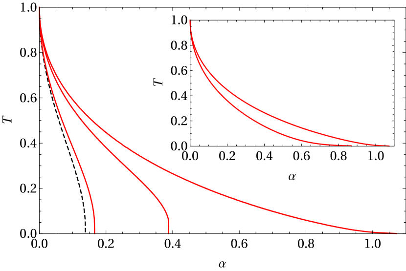
Figure 1: Critical line for the transition between retrieval and spin-glass phases for various values of the unlearning time. From the left to the right: $t=0$ (Hopfield, black dashed line), $0.1$, $1$ and $1000$. The inset shows two curves tracing the boundary of the maximal retrieval regions where patterns are global free energy minima (inner boundary) or local free energy minima (outer boundary) in the long sleep limit.

2 Replica symmetric free energy analysis

2.1 Definition of the Model

Driven by the works of Personnaz, Guyon, Dreyfus Personnaz and of Dotsenko et al. Dotsenko1 ; Dotsenko2 , in Albert2 we introduced the following generalization of the standard Hopfield paradigma Hopfield , referred to as “reinforcement&removal” (RR) algorithm: consider a network composed by $N$ Ising neurons $\{\sigma_{i}\}_{i=1,...,N}$ and $P$ patterns $\{\xi^{\mu}\}_{\mu=1,...,P}$ (namely quenched random vectors of the same length $N$), and denote with $t\in\mathbb{R}^{+}$ the sleep extent (such that for $t=0$ the network has never slept, while for $t\to\infty$ an entire sleeping session has occurred), we can then introduce the following

Definition 1.

The Hamiltonian of the reinforcement$\&$removal model reads as:

$$H_{N,P}^{\textrm{(RR)}}(\sigma|\xi,t):=-\frac{1}{2N}\sum_{i=1}^{N}\sum_{j=1}^{N}\sum_{\mu=1}^{P}\sum_{\nu=1}^{P}\xi_{i}^{\mu}\xi_{j}^{\nu}\left(\frac{1+t}{\mathbb{I}+tC}\right)_{\mu,\nu}\sigma_{i}\sigma_{j},$$ (1)

where $\sigma_{i}=\pm 1\ \forall i\in(1,...,N)$, $\xi^{1}$ -that is the pattern candidate to be retrieved- has binary entries $\xi_{i}^{1}\in\{-1,+1\}$ drawn from $P(\xi_{i}^{\mu}=+1)=P(\xi_{i}^{\mu}=-1)=\frac{1}{2}$, while the remaining $P-1$ patterns $\{\xi^{\mu}\}_{\mu=2,...,P}$, have i.i.d. standard Gaussian entries $\xi_{i}^{\mu}\sim\mathcal{N}[0,1]$, and the correlation matrix $\boldsymbol{C}$ is defined as

$$C_{\mu,\nu}:=\frac{1}{N}\sum_{i=1}^{N}\xi_{i}^{\mu}\xi_{i}^{\nu}.$$

Remark 1.

We stress that, for the sake of mathematical convenience, as deepened in Agliari-Barattolo , we take solely the pattern candidate for retrieval (i.e. the signal) to be Boolean, while all the remaining ones (acting as slow noise on the retrieval) are chosen as Gaussian: although neural networks, in general, do not exhibit the universality properties of spin glasses Genovese , this is no longer true if we confine our focus solely to the structure of the slow noise generated by patterns.

Remark 2.

Note that the matrix ${\xi}^{T}\left(\frac{1+t}{\mathbb{I}+t{C}}\right){\xi}$, encoding the neuronal coupling, recovers the Hebbian kernel for $t=0$ , while it approaches the pseudo-inverse matrix for $t\rightarrow\infty$ (see Albert2 for the proof). Accordingly, the model described by the Hamiltonian (1) spans, respectively, from the standard Hopfield model $(t\to 0)$ to the Kanter-Sompolinksy model KanterSompo $(t\to\infty)$.
During the sleeping session, both reinforcement and remotion take place: oversimplifying, in the generalized synaptic coupling appearing in (1), the denominator (i.e., the term $\propto(1+tC)^{-1}$) yields to the remotion of unwanted mixture states, while the numerator (i.e., the term $\propto 1+t$) reinforces the pure memories.

We are interested in obtaining the phase diagram of the model coded by the cost function (1), solely in the thermodynamic limit and under the replica symmetric assumption. To achieve this goal the following definitions are in order.

Definition 2.

Using $\beta\in\mathbb{R}^{+}$ as a parameter tuning the level of fast noise in the network (with the physical meaning of inverse temperature, i.e. calling $T$ the temperature, $\beta\equiv T^{-1}$ in proper units,), the partition function of the model (1) is introduced as

$$Z_{N,P}(\sigma|\xi,t):=\sum_{\{\sigma\}}e^{-\beta H_{N,P}^{(RR)}(\sigma|\xi,t)}=\sum_{\{\sigma\}}\exp\left[\frac{\beta}{2N}\sum_{i,j=1}^{N,N}\sum_{\mu,\nu=1}^{P,P}\xi^{\mu}_{i}\xi^{\nu}_{j}\left(\frac{1+t}{\mathbb{I}+tC}\right)_{\mu,\nu}\sigma_{i}\sigma_{j}\right].$$ (2)

Definition 3.

Denoting with $\mathbb{E}_{\xi}$ the average over the quenched patterns, for a generic function $O(\sigma,\xi)$ of the neurons and the couplings, we can define the Boltzmann $\langle O(\sigma,\xi)\rangle$ as

$$\langle O(\sigma,\xi)\rangle := \frac{\sum_{\{\sigma\}}O(\sigma,\xi)e^{-\beta H^{(RR)}_{N,P}(\sigma|\xi,t)}}{Z_{N,P}(\sigma|\xi,t)},$$ (3)

such that its quenched average reads as $\mathbb{E}_{\xi}\langle O(\sigma,\xi)\rangle$.

Definition 4.

Once introduced the partition function $Z_{N,P}(\sigma|\xi,t)$, we can define the infinite volume limit of the intensive quenched free-energy $F_{N}(\alpha,\beta,t)$ and of the intensive quenched pressure $A(\alpha,\beta,t)$ associated to the model (1) as

$$-\beta F(\alpha,\beta,t)\equiv A(\alpha,\beta,t):=\lim_{N\to\infty}\frac{1}{N}\mathbb{E}\ln Z_{N,P}(\sigma|\xi,t).$$ (5)

As anticipated, the pressure of the model (1) was analyzed in Albert2 via replica-trick Coolen (corroborated by extensive numerical simulations), showing that (at the replica symmetric level of description) the maximal critical capacity of this neural network saturates the Gardner’s bound Gardner (i.e. $\alpha_{c}=1$, for symmetric noiseless networks).

Remark 3.

The partition function defined in (2) can be represented in Gaussian integral form as

$$\begin{split}Z_{N,P}(\sigma|\xi,t)&=\sum_{\{\sigma\}}\int\Big{(}\prod_{\mu=1}^{P}d\mu(z_{\mu})\Big{)}\Big{(}\prod_{i=1}^{N}d\mu(\phi_{i})\Big{)}\cdot\\ &\cdot\exp\left(\sqrt{\frac{\beta}{N}(t+1)}\sum_{\mu,i}^{P,N}z_{\mu}\xi^{\mu}_{i}\sigma_{i}+i\sqrt{\frac{t}{N}}\sum_{\mu,i}^{P,N}z_{\mu}\xi^{\mu}_{i}\phi_{i}\right),\end{split}$$ (6)

where $d\mu(z_{\mu})$ and $d\mu(\phi_{i})$ are the standard Gaussian measures. This relation shows that the partition function of the reinforcement$\&$removal model is equivalent to the partition function of a tripartite spin-glass where the intermediate party (or hidden layer to keep a machine learning jargon) is made of real neurons $\{z_{\mu}\}_{\mu=1,...,P}$ with $z_{\mu}\sim\mathcal{N}[0,1],\forall\mu$, while the external layers are made, respectively, of a set of Boolean neurons $\{\sigma_{i}\}_{i=1,...,N}$ (the visible layer) and of a set of imaginary neurons with magnitude $\{\phi\}_{i=1,...,N}$, being $\phi_{i}\sim\mathcal{N}[0,1],\forall i$ (the spectral layer), see Fig. 2.

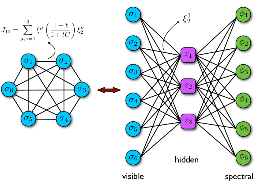
Figure 2: Stylized representation of the generalized Hopfield network (left) and its dual generalized (restricted) Boltzmann machine (right), namely the three-partite spin-glass under study: in machine learning jargon these parties are called layers and, here, they are respectively the visible, hidden and spectral layers. Note further that, as it should, when $t\to 0$ the duality above reduces to the standard picture of Hopfield networks and restricted Boltzmann machines Agliari-Barattolo ; BarraEquivalenceRBMeAHN .

2.2 Guerra’s interpolating framework for the free energy

Definition 5.

Once expressed the partition function (2) in its integral representation (6), we can introduce the related tripartite spin glass Hamiltonian as

$$H_{N,P}=\frac{a}{\sqrt{N}}\sum_{i=1}^{N}\sum_{\mu=1}^{P}z_{\mu}\xi_{i}^{\mu}k_{i},$$ (7)

where we introduced the “multi-spin” $k_{i}=\sigma_{i}+b\phi_{i}$ and where

$$a=\sqrt{\beta(t+1)},\quad b=i\sqrt{\frac{t}{\beta(t+1)}}.$$ (8)

Remark 4.

Note that the cost function (7) and the one associated to the original model (1) share the same partition function and therefore exhibit the same Thermodynamics. By a practical perspective, the latter is more suitable for understanding the retrieval capabilities of the network, the former for dealing with its learning skills BarraEquivalenceRBMeAHN ; Barra-RBMsPriors1 .

In the following we consider the challenging case with $P=\alpha N$ for large $N$ and we aim to obtain an expression for the quenched pressure (5) in terms of the order parameters introduced in the next

Definition 6.

The natural order parameters for the neural network model (1) -as suggested by its integral representation (7)- are the overlaps $q_{ab}$ and $p_{ab}$ between the $k$’s and the $z$’s variables, respectively, as functions of two replicas (a,b) of the system, and the generalized Mattis overlap $m_{1}$, namely

$$\begin{split}q_{ab}&:=\frac{1}{N}\sum_{i=1}^{N}k_{i}^{(a)}k_{i}^{(b)},\\ p_{ab}&:=\frac{1}{P}\sum_{\mu\geq 2}z_{\mu}^{(a)}z_{\mu}^{(b)},\\ m_{1}&:=\frac{1}{N}\sum_{i=1}^{N}\xi_{i}^{1}k_{i}.\end{split}$$ (9)

Remark 5.

The replica symmetric approximation (RS) is imposed by requiring that the order-parameters of the theory do not fluctuate in the thermodynamic limit, i.e.

$$\begin{split}q_{ab}&\overset{\rm\scriptscriptstyle RS}{\to}W\delta_{ab}+q(1-\delta_{ab}),\\ p_{ab}&\overset{\rm\scriptscriptstyle RS}{\to}X\delta_{ab}+p(1-\delta_{ab}),\\ m_{1}&\overset{\rm\scriptscriptstyle RS}{\to}m,\end{split}$$ (10)

where we called, respectively, $W,q,X,p,m$ the replica symmetric values of the diagonal and off-diagonal overlap $q$, the diagonal and off-diagonal overlap $p$ and the Mattis magnetization $m_{1}$.

Now the plan is to get an explicit expression for the pressure (5) in terms of these order parameters, to extremize the former over the latter and get a phase diagram for the network. To reach this goal we generalize a Guerra’s interpolation scheme Barra-JSP2010 : the idea is to compare the original system, as represented in eq. (7) (namely a three-layer correlated spin glass), with three random single-layers, where each layer experiences, statistically, the same mean-field that would have been produced by the other layers over it. To this aim we introduce the following

Definition 7.

Being $s\in[0,1]$ an interpolating parameter, $\{\eta_{i}\}_{i\in(1,...,N)}$ a set of $N$ i.i.d. Gaussian variables, $\{\lambda_{\mu}\}_{\mu\in(2,...,P)}$ a set of $P-1$ i.i.d. Gaussian variables, and the scalars $C_{1},C_{2},C_{3},C_{4},C_{5}$ to be set a posteriori, we use as interpolating pressure the following quantity

$$\mathcal{A}(s) := \frac{1}{N}\operatorname{\mathbb{E}_{\xi,\eta,\lambda}}\ln\sum_{\sigma}\int\!\operatorname{d\mu}\left(z,\phi\right)\exp\Big{[}\sqrt{s}\frac{a}{\sqrt{N}}\sum_{i,\mu\geq 2}z_{\mu}\xi_{i}^{\mu}k_{i}+\sqrt{s}\frac{a}{\sqrt{N}}\sum_{i}z_{1}\xi_{i}^{1}k_{i}$$

$$+ \sqrt{1-s}\Big{(}C_{1}\sum_{i}^{N}\eta_{i}k_{i}+C_{2}\sum_{\mu\geq 2}\lambda_{\mu}z_{\mu}\Big{)}+\frac{1-s}{2}\Big{(}C_{3}\sum_{\mu\geq 2}z_{\mu}^{2}+C_{4}\sum_{i}k_{i}^{2}+C_{5}a\sum_{i}\xi_{i}^{1}k_{i}\Big{)}\Big{]}.$$

Remark 6.

When $s=1$ we recover the original model, namely $A(\alpha,\beta,t)=\lim_{N\to\infty}\mathcal{A}(s=1)$, while for $s\to 0$ we are left with a one-body problem, and, consequently, the probabilistic structure of $\mathcal{A}(s=0)$ is more tractable.

Remark 7.

We note the importance of splitting the sum on the $\xi$’s into $\xi^{1}$ (i.e. the signal) and the $\xi^{2}\cdots\xi^{P}$ (i.e. the quenched noise) since the quenched average treats them differently, and so we will need to address them separately.

Proposition 1.

The infinite volume limit of the quenched pressure related to the model (1) can be obtained by using the Fundamental Theorem of Calculus as

$$A(\alpha,\beta,t)\equiv\lim_{N\to\infty}\mathcal{A}(s=1)=\lim_{N\to\infty}\left(\mathcal{A}(s=0)+\int_{0}^{1}\frac{d\mathcal{A}(s)}{ds}\,ds\right).$$ (12)

To follow this approach, two calculations are in order: the streaming $d_{s}\mathcal{A}(s)$ (and its successive back-integration) and the evaluation of the Cauchy condition $\mathcal{A}(s=0)$. Let us start with $d_{s}\mathcal{A}(s)$:

$$\begin{split}\frac{d\mathcal{A}(s)}{ds}=&\frac{1}{2N}\operatorname{\mathbb{E}_{\xi,\lambda,\eta}}\Big{[}\frac{a}{\sqrt{sN}}\sum_{i,\mu\geq 2}\xi_{i}^{\mu}\langle z_{\mu}k_{i}\rangle-\frac{1}{\sqrt{1-s}}\Big{(}C_{1}\sum_{i}\eta_{i}\langle k_{i}\rangle+C_{2}\sum_{\mu\geq 2}\lambda_{\mu}\langle z_{\mu}\rangle\Big{)}+\\ &+\frac{a}{\sqrt{sN}}\sum_{i}\xi_{i}^{1}\langle z_{1}k_{i}\rangle-C_{3}\sum_{\mu\geq 2}\langle z_{\mu}^{2}\rangle-C_{4}\sum_{i}\langle k_{i}^{2}\rangle-C_{5}a\sum_{i}\langle\xi_{i}^{1}k_{i}\rangle\Big{]}.\end{split}$$ (13)

We can proceed further by using Wick’s Theorem [$\mathbb{E}_{x}xF(x)=\mathbb{E}_{x}(x^{2})\cdot\mathbb{E}_{x}\partial_{x}F(x)$] on the fields $z^{1},\,\,\xi^{2\cdots P},\,\,\lambda_{\mu},\,\,\eta_{i}$, obtaining

$$\begin{split}\frac{d\mathcal{A}(s)}{ds}=&\frac{1}{2N}\operatorname{\mathbb{E}_{\xi,\lambda,\eta}}\Big{[}\frac{a^{2}}{N}\sum_{i,\mu\geq 2}\Big{(}\langle z_{\mu}^{2}k_{i}^{2}\rangle-\langle z_{\mu}k_{i}\rangle^{2}\Big{)}+\frac{a^{2}}{N}\langle\big{(}\sum_{i}\xi_{i}^{1}k_{i}\big{)}^{2}\rangle-C_{1}^{2}\sum_{i}\Big{(}\langle k_{i}^{2}\rangle-\langle k_{i}\rangle^{2}\Big{)}\\ &-C_{2}^{2}\sum_{\mu\geq 2}\Big{(}\langle z_{\mu}^{2}\rangle-\langle z_{\mu}\rangle^{2}\Big{)}-C_{3}\sum_{\mu\geq 2}\langle z_{\mu}^{2}\rangle-C_{4}\sum_{i}\langle k_{i}^{2}\rangle-C_{5}a\sum_{i}\langle\xi_{i}^{1}k_{i}\rangle\Big{]}.\end{split}$$ (14)

Using the definition of the order parameters (9) we can write $d_{s}\mathcal{A}(s)$ as

$$\begin{split}\frac{d\mathcal{A}(s)}{ds}=&\frac{1}{2}\operatorname{\mathbb{E}_{\xi,\lambda,\eta}}\Big{[}a^{2}\alpha\langle q_{11}p_{11}\rangle+a^{2}\langle m_{1}^{2}\rangle-a^{2}\alpha\langle q_{12}p_{12}\rangle-C_{1}^{2}\langle q_{11}\rangle+C_{1}^{2}\langle q_{12}\rangle+\\ &-C_{2}^{2}\alpha\langle p_{11}\rangle+C_{2}^{2}\alpha\langle p_{12}\rangle-\alpha C_{3}\langle p_{11}\rangle-C_{4}\langle q_{11}\rangle-aC_{5}\langle m_{1}\rangle\Big{]}.\end{split}$$ (15)

It is now convenient to fix the free scalars $C_{1,..,5}$ as

$$C_{1}^{2}=a^{2}\alpha p,\quad C_{2}^{2}=a^{2}q,\quad C_{3}=a^{2}(W-q),\quad C_{4}=a^{2}\alpha(X-p),\quad C_{5}=2ma,$$ (16)

such that we can recast the streaming $d_{s}\mathcal{A}(s)$ as

$$\begin{split}\frac{d\mathcal{A}(s)}{ds}=&\frac{1}{2}\operatorname{\mathbb{E}_{\xi,\lambda,\eta}}\Big{[}a^{2}\alpha\langle(q_{11}-W)(p_{11}-X)\rangle+a^{2}\langle(m_{1}-m)^{2}\rangle-a^{2}\alpha\langle(q_{12}-q)(p_{12}-p)\rangle\Big{]}+\\ &+\frac{\alpha a^{2}}{2}(qp-WX)-\frac{a^{2}}{2}m^{2}.\end{split}$$ (17)

Remark 8.

When requiring replica symmetry, we have that $\langle q_{11}\rangle\to W$, $\langle p_{11}\rangle\to X$, $\langle m_{1}\rangle\to m$, $\langle q_{12}\rangle\to q$ and $\langle p_{12}\rangle\to p$, hence the evaluation of the integral in eq. (12) becomes trivial as the r.h.s. of eq. (17) reduces to

$$\begin{split}d_{s}\mathcal{A}(s)=\frac{\alpha a^{2}}{2}(qp-WX)-\frac{a^{2}}{2}m^{2}\end{split}$$ (18)

that does not depend on $s$ any longer.

We must now evaluate the one-body contribution $\mathcal{A}(s=0)$: this can be done by directly setting $s=0$ in (7)

$$\begin{split}\mathcal{A}(s=0)=&\frac{1}{N}\operatorname{\mathbb{E}_{\xi,\eta,\lambda}}\ln\sum_{\sigma}\int\!\operatorname{d\mu}\left(z,\phi\right)\exp\Big{[}C_{1}\sum_{i}\eta_{i}k_{i}+\frac{C_{4}}{2}\sum_{i}k_{i}^{2}+\frac{C_{5}a}{2}\sum_{i}\xi_{i}^{1}k_{i}+\\ &+C_{2}\sum_{\mu\geq 2}\lambda_{\mu}z_{\mu}+\frac{C_{3}}{2}\sum_{\mu\geq 2}z_{\mu}^{2}\Big{]}.\end{split}$$ (19)

Performing standard Gaussian integrations we obtain

$$\begin{split}\mathcal{A}(s=0)=&-\frac{\alpha}{2}\ln(1-C_{3})-\frac{1}{2}\ln(1-C_{4}b^{2})+\frac{\alpha}{2}\frac{C_{2}^{2}}{1-C_{3}}+\frac{C_{4}}{2}+\operatorname{\mathbb{E}_{\eta}}\ln\cosh\Big{[}\frac{C_{1}\eta+\frac{C_{5}a}{2}}{1-C_{4}b^{2}}\Big{]}+\\ &+b^{2}\frac{C_{1}^{2}+C_{4}^{2}+\frac{C_{5}^{2}a^{2}}{4}}{1-C_{4}b^{2}}+\ln 2.\end{split}$$ (20)

Keeping in mind the expressions for the parameters $C_{1},...,C_{5}$ as prescribed in the relations 16, by plugging eq. (18) and eq. (20) into the sum rule (12) we finally get an expression for the quenched pressure of the model (1) in terms of the replica-symmetric order parameters

$$\begin{split}A_{{\rm\scriptscriptstyle RS}}(\alpha,\beta,t)=&\frac{\alpha a^{2}}{2}\big{(}qp-WX\big{)}-\frac{a^{2}}{2}m^{2}-\frac{\alpha}{2}\ln\big{[}1-a^{2}(W-q)\big{]}-\frac{1}{2}\ln\big{[}1-a^{2}b^{2}\alpha(X-p)\big{]}+\\ &+\frac{\alpha}{2}\frac{a^{2}q}{1-a^{2}(W-q)}+\frac{\alpha a^{2}}{2}\big{(}X-p\big{)}+\frac{a^{2}b^{2}}{2}\cdot\frac{\alpha p+m^{2}a^{2}+a^{2}\alpha^{2}(X-p)^{2}}{1-a^{2}b^{2}\alpha(X-p)}+\\ &+\ln 2+\operatorname{\mathbb{E}_{\eta}}\ln\cosh\Big{[}\frac{a\eta\sqrt{\alpha p}+ma^{2}}{1-\alpha a^{2}b^{2}(X-p)}\Big{]}.\end{split}$$ (21)

To match exactly the notation in Albert2 there is still a short way to go: it is convenient to re-scale $m$, $p$ and $X$ as

$$X\to\frac{\beta^{2}}{a^{2}}X,\quad p\to\frac{\beta^{2}}{a^{2}}p,\quad m\to\frac{\beta}{a^{2}}m,$$ (22)

as this allows us to introduce the composite order parameter $\Delta=1-\alpha\beta^{2}b^{2}(X-p)$ used in Albert2 .
After these transformations, remembering the definition of the free energy (see (5)) and the definition of $(a,b)$ (see (8)), we obtain exactly the same expression for the quenched free energy as that achieved in Albert2 via the replica trick, as stated by the next main

Theorem 1.

In the infinite volume limit, the replica symmetric free energy related to the neural network defined by eq. (1) can be expressed in terms of the natural order parameters of the theory (see def.s (9)) as

$$\begin{split}F_{{\rm\scriptscriptstyle RS}}(\alpha,\beta,t)=&-\frac{\beta m^{2}}{2(1+t)}\Big{(}1+\frac{t}{\Delta}\Big{)}-\frac{(1+t)(\Delta-1)}{2t}\beta W-\frac{\alpha\beta^{2}}{2}p(W-q)\\ &-\frac{\alpha}{2}\Big{(}\log[1-\beta(1+t)(W-q)]+\frac{q\beta^{2}(1+t)}{1-\beta(1+t)(W-q)}\Big{)}-\frac{(1+t)(1-\Delta)\beta}{2t\Delta}\\ &-\frac{\log\Delta}{2}-\frac{\alpha\beta pt}{2(1+t)\Delta}+\operatorname{\mathbb{E}_{\eta}}\log\cosh\Big{[}\frac{\beta}{\Delta}(m+\sqrt{\alpha p}\eta)\Big{]}+\log 2.\end{split}$$ (23)

Proposition 2.

Using the standard variational principle $\vec{\nabla}F_{{\rm\scriptscriptstyle RS}}=0$ on the free energy (23), namely by extremizing the latter over the order parameters, we obtain the following set of self-consistent equations for these parameters, whose behavior is outlined in the plots of Fig. 3.

$$\begin{split}m&=\frac{1+t}{\Delta+t}\operatorname{\mathbb{E}_{\eta}}\tanh\Big{[}\frac{\beta}{\Delta}(m+\sqrt{\alpha p}\eta)\Big{]},\\ p&=\frac{q(1+t)^{2}}{[1-\beta(1+t)(W-q)]^{2}},\\ \Delta&=1+\frac{\alpha t}{1-\beta(1+t)(W-q)},\\ q&=W+\frac{t}{\beta(1+t)\Delta}-\frac{1}{\Delta^{2}}\operatorname{\mathbb{E}_{\eta}}\cosh^{-2}\Big{[}\frac{\beta}{\Delta}(m+\sqrt{\alpha p}\eta)\Big{]},\\ W\Delta^{2}&=1-\frac{t\Delta}{\beta(1+t)}+\frac{\alpha pt^{2}-m^{2}t(t+2\Delta)}{(1+t)^{2}}-\frac{2\alpha\beta pt}{(1+t)\Delta}\operatorname{\mathbb{E}_{\eta}}\cosh^{-2}\Big{[}\frac{\beta}{\Delta}(m+\sqrt{\alpha p}\eta)\Big{]}.\end{split}$$ (24)

Remark 9.

We stress that we obtained exactly the same self-consistencies previously appeared in Albert2 , thus all the consequences stemming by them, as reported in that paper, are here entirely confirmed.

Figure 3: Retrieval state solution for the order parameters and free energy at $t=1000$. First row: on the left, the plot shows the Mattis magnetization $m$ as a function of the temperature for various storage capacity values ($\alpha=0$, $0.05$, $0.2$ and $0.5$, going from the right to the left). The vertical dotted lines indicates the jump discontinuity identifying the critical temperature $T_{c}(\alpha)$ which separates the retrieval region from the spin-glass phase; on the right, the plot shows the solutions of the non-diagonal overlap $q$ (normalized to the zero-temperature value $q_{0}=q(T=0)$), for the same capacity values. The solution is computed in the retrieval region (i.e. $T<T_{c}(\alpha)$). Second row: on the left, the plot shows the solution for the diagonal overlap $-W$ in the retrieval region for $\alpha=0$, $0.05$, $0.2$ and $0.5$, finally, on the right the plot shows the free-energy as a function of the temperature for various storage capacity values ($\alpha=0.05$, $0.2$ and $0.5$, going from the bottom to the top) for both the retrieval (red solid lines) and spin-glass (black dashed lines) states.

3 Study of the overlap fluctuations

As proved in the previous section, the reinforcement$\&$removal algorithm makes the retrieval region in the $(\alpha,\beta)$ plane wider and wider as $t$ is increased (see Fig. 1). As the retrieval region pervades the spin-glass region, one therefore naturally wonders whether the opposite boundary of the spin-glass region (namely the critical line depicting the transition where ergodicity breakdowns) is as well deformed. To address this point, we now study the behavior of the overlap fluctuations, suitably centered around the thermodynamic values of the overlaps and properly rescaled in order to allow them to diverge when the system approaches the critical line. In fact, they are meromorphic functions and their poles identify the evolution of the critical surface $\beta_{c}(\alpha,t)$ (if any).
It is worth recalling that the critical line for the standard Hopfield model Hopfield as predicted by the AGS theory Amit is $\beta_{c}(\alpha,t=0)=(1+\sqrt{\alpha})^{-1}$.

3.1 Guerra’s interpolating framework for the overlap fluctuations

The idea is the same exploited in the previous section, namely to use the generalized Guerra’s interpolation scheme (see eq. (7)) to evaluate the evolution of the order parameter’s correlation functions from $s=0$ (where they do not represent the real fluctuations in the system, but their evaluation should be possible) up to $s=1$ (where they reproduce the true fluctuations). To achieve this goal for the generic correlation function $O$, we need to evaluate the Cauchy condition $\langle O(s=0)\rangle$ and the derivative $\partial_{s}\langle O(s)\rangle$. However, in contrast with the previous section where we imposed replica symmetry, here -as we just want to infer the critical line- we impose ergodic behavior, namely, we assume that the system is approaching this boundary from the high fast-noise limit. This allows us to set all the mean values of the overlaps to zero and to achieve explicit solutions.

Definition 8.

The centered and rescaled overlap fluctuations $\theta_{lm}$ and $\rho_{lm}$ are introduced as

$$\begin{split}\theta_{lm}&=\sqrt{N}\big{[}q_{lm}-\delta_{lm}W-(1-\delta_{lm})q\big{]}\\ \rho_{lm}&=\sqrt{P}\big{[}p_{lm}-\delta_{lm}X-(1-\delta_{lm})p\big{]}.\end{split}$$ (25)

Remark 10.

As we will address the problem of the overlap fluctuations in the ergodic region, the signal is absent, thus there is no need to introduce a rescaled Mattis order parameter: only the boundary between the ergodic region and the spin-glass region is under study here.

Proposition 3.

It is convenient to introduce the $r-$replicated interpolating pressure $\mathcal{A}_{J}^{r}(s)$, where we further added a source field $J$, coupled to an observable $O$ (that is a smooth function of the neurons of the $r$-replicas) as

$$\begin{split}\mathcal{A}^{r}_{J}(s)=&\operatorname{\mathbb{E}_{\xi,\eta,\lambda}}\ln\sum_{\sigma_{R}}\int\!\operatorname{d\mu}\left(z_{R},\phi_{R}\right)\exp\Big{[}\sqrt{s}\frac{a}{\sqrt{N}}\sum_{l=1}^{r}\sum_{i,\mu}z_{\mu}^{(l)}\xi_{i}^{\mu}k_{i}^{(l)}+J\hat{O}\\ &+\sqrt{1-s}\Big{(}C_{1}\sum_{l=1}^{r}\sum_{i}\eta_{i}k_{i}^{(l)}+C_{2}\sum_{l=1}^{r}\sum_{\mu}\lambda_{\mu}z_{\mu}^{(l)}\Big{)}+\frac{1-s}{2}\Big{(}C_{3}\sum_{l=1}^{r}\sum_{\mu}(z_{\mu}^{(l)})^{2}+C_{4}\sum_{l=1}^{r}\sum_{i}(k_{i}^{(l)})^{2}\Big{)}\Big{]}.\end{split}$$ (26)

where $k_{i}$ is the same as in Definition $5$ and the interpolation constants $C_{1,2,3,4}$ are the same given in the previous section (see eq. ((16))).

By definition

$$\langle O(s)\rangle=\left.\frac{\partial\mathcal{A}^{r}_{J}(s)}{\partial J}\right|_{J=0},\quad\quad\partial_{s}\langle O(s)\rangle=\left.\frac{\partial(\partial_{s}\mathcal{A}^{r}_{J})}{\partial J}\right|_{J=0}.$$ (27)

Therefore, in order to evaluate the fluctuations of $O$ we need to evaluate first $\partial_{s}\mathcal{A}^{r}_{J}$ and, by a routine calculation, we get

$$\partial_{s}\mathcal{A}^{r}_{J}=\frac{1}{2}\sqrt{\alpha}\beta(1+t)\sum_{l,m=1}^{r}\Big{[}\langle g_{l,m}\rangle-\langle g_{l,m+r}\rangle\Big{]},\quad\quad g_{l,m}=\theta_{l,m}\rho_{l,m}.$$ (28)

To evaluate the fluctuations of a general operator $O$, function of $r-$replicas, we must use the results (27) and perform the same rescaling that we did in the previous section, namely

$$(X,p)\to\frac{\beta^{2}}{a^{2}}(X,p).$$ (29)

Overall this brings to the next

Proposition 4.

Given $O$ as a smooth function of $r$ replica overlaps $\left(q_{1},\ldots,q_{r}\right)$ and $\left(p_{1},\ldots,p_{r}\right),$ the following streaming equation holds:

$$d_{\tau}\langle O\rangle=\frac{1}{2}\sum_{a,b}^{r}\langle O\cdot g_{a,b}\rangle-r\sum_{a=1}^{r}\langle O\cdot g_{a,r+1}\rangle+\frac{r(r+1)}{2}\langle O\cdot g_{r+1,r+2}\rangle-\frac{r}{2}\langle O\cdot g_{r+1,r+1}\rangle,$$ (30)

where we used the operator $d_{\tau}$ defined as

$$d_{\tau}=\frac{1}{\beta(1+t)\sqrt{\alpha}}\frac{d}{ds},$$ (31)

in order to simplify calculations and presentation.

3.2 Criticality and ergodicity breaking

To study the overlap fluctuations we must consider the following correlation functions (it is useful to introduce and link them to capital letters in order to simplify their visualization):

$$\begin{split}\langle\theta_{12}^{2}\rangle_{s}&=A(s),&\langle\theta_{12}\theta_{13}\rangle_{s}&=B(s),&\langle\theta_{12}\theta_{34}\rangle_{s}&=C(s),\\ \langle\theta_{12}\rho_{12}\rangle_{s}&=D(s),&\langle\theta_{12}\rho_{13}\rangle_{s}&=E(s),&\langle\theta_{12}\rho_{34}\rangle_{s}&=F(s),\\ \langle\rho_{12}^{2}\rangle_{s}&=G(s),&\langle\rho_{12}\rho_{13}\rangle_{s}&=H(s),&\langle\rho_{12}\rho_{34}\rangle_{s}&=I(s),\\ \langle\theta_{11}^{2}\rangle_{s}&=J(s),&\langle\theta_{11}\rho_{11}\rangle_{s}&=K(s),&\langle\rho_{11}^{2}\rangle_{s}&=L(s),\\ \langle\theta_{11}\theta_{12}\rangle_{s}&=M(s),&\langle\theta_{11}\rho_{12}\rangle_{s}&=N(s),&\langle\rho_{11}\theta_{12}\rangle_{s}&=O(s),\\ \langle\rho_{11}\rho_{12}\rangle_{s}&=P(s),&\langle\theta_{11}\rho_{22}\rangle_{s}&=Q(s),&\langle\theta_{11}\theta_{22}\rangle_{s}&=R(s).\\ \langle\rho_{11}\rho_{22}\rangle_{s}&=S(s),\end{split}$$ (32)

Since we are interested in finding the critical line for ergodicity breaking from above we can treat $\theta_{a,b},\rho_{a,b}$ as Gaussian variables with zero mean (this allows us to apply Wick-Isserlis theorem inside averages) as we can also treat both the $k_{i}$ and $z_{\mu}$ as zero mean random variables in the ergodic region (thus all averages involving uncoupled fields are vanishing): this considerably simplifies the evaluation of the critical line (as expected since we are approaching criticality from the trivial ergodic region BarraGuerra-JMP2008 ).
We can thus reduce the analysis to

$$\begin{split}\langle\theta_{12}^{2}\rangle_{s}&=A(s),&\langle\theta_{12}\rho_{12}\rangle_{s}&=D(s),&\langle\rho_{12}^{2}\rangle_{s}&=G(s),\\ \langle\theta_{11}^{2}\rangle_{s}&=J(s),&\langle\theta_{11}\rho_{11}\rangle_{s}&=K(s),&\langle\rho_{11}^{2}\rangle_{s}&=L(s),\\ \langle\theta_{11}\rho_{22}\rangle_{s}&=Q(s),&\langle\theta_{11}\theta_{22}\rangle_{s}&=R(s),&\langle\rho_{11}\rho_{22}\rangle_{s}&=S(s).\end{split}$$ (33)

According to (30) and to the previous reasoning we obtain:

$$\begin{split}d_{\tau}{A}&=2AD,\\ d_{\tau}{D}&=D^{2}+AG,\\ d_{\tau}{G}&=2GD.\end{split}$$ (34)

Suitably combining $A$ and $G$ in (34) we can write

$$d_{\tau}\ln\frac{A}{G}=0\implies A(\tau)=r^{2}G(\tau),\quad r^{2}=\frac{A(0)}{G(0)}.$$ (35)

Now we are left with

$$\begin{split}d_{\tau}{D}&=D^{2}+r^{2}G^{2},\\ d_{\tau}{G}&=2GD.\end{split}$$ (36)

The trick here is to complete the square by summing $d_{\tau}D+rd_{\tau}G$ thus obtaining

$$\begin{split}d_{\tau}Y&=Y^{2},\\ Y&=D+rG,\\ d_{\tau}{G}&=2G(Y-rG).\end{split}$$ (37)

The solution is trivial and it is given by

$$Y(\tau)=\frac{Y_{0}}{1-\tau Y_{0}},\quad Y_{0}=D(0)+\sqrt{A(0)G(0)}.$$ (38)

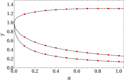
Figure 4: Ergodicity breaking critical line. The plot shows a comparison between the theoretical predictions (black dashed lines) for the ergodicity breaking critical line according to Eq. (44) and numerical solutions for spin glass states (red markers). The latter are evaluated by solving the self-consistency equations with $m=0$ with $\alpha$ fixed and searching for the temperature $T$ above which the solution has $q=0$. Going from top to bottom of the plot, the sleep extent is $t=0.1$, $1$ and $2$.

So we are left with the evaluation of the correlations at $s=0$: namely the Cauchy conditions related to the solution coded in eq. (38). To this task we introduce a one-body generating function for the momenta of $z,k$: this can be done by setting inside (26) $s=0,r=1$ and adding source fields $(j_{i},J_{\mu})$ coupled respectively to $(k_{i},z_{\mu})$, with $i\in(1,...,N),\,\mu\in(1,...,P)$. Since we are approaching the critical line from the high fast noise limit we can set $m,p,q=0$ (when we explicitly make use of the coefficients (16)), overall writing

$$\begin{split}F(j,J)=&\ln\sum_{\sigma}\int\!\operatorname{d\mu}\left(z,\phi\right)\exp\Big{[}\sum_{i}j_{i}k_{i}+\sum_{\mu}J_{\mu}z_{\mu}+\frac{a^{2}W}{2}\sum_{\mu}z_{\mu}^{2}+\frac{1-\Delta}{2b^{2}}\sum_{i}k_{i}^{2}\Big{]}.\end{split}$$ (39)

Clearly, we took great advantage in approaching the ergodic region from above, since even the one-body problem (for the Cauchy condition) has been drastically simplified: showing only the relevant terms in $j,J$ we have

$$\begin{split}F(j,J)=\frac{b^{2}\Delta+1}{2\Delta^{2}}\sum_{i}j_{i}^{2}+\frac{1}{2(1-a^{2}W)}\sum_{\mu}J_{\mu}^{2}+O(j^{3}).\end{split}$$ (40)

As anticipated, all the observable averages needed at $s=0$ can now be calculated simply as derivatives of $F(j,J)$, thus the $s=0$ correlation functions are finally given by

$$\begin{split}D(0)&=\sqrt{NP}\left.\big{(}\partial_{j}F\big{)}^{2}\big{(}\partial_{J}F\big{)}^{2}\right|_{j,J=0}=0,\\ A(0)&=\left.\big{(}\partial^{2}_{j}F\big{)}^{2}\right|_{j,J=0}=\Big{[}\frac{\beta(1+t)-t\Delta}{\beta(1+t)\Delta^{2}}\Big{]}^{2}=W^{2},\\ G(0)&=\left.\big{(}\partial^{2}_{J}F\big{)}^{2}\right|_{j,J=0}=(1-\beta(1+t)W)^{-2}.\end{split}$$ (41)

Inserting this result in (38), we get

$$\begin{split}Y(\tau)=\frac{W}{1-\beta(1+t)W-\tau W}.\end{split}$$ (42)

Upon evaluating $Y(\tau)$ for $\tau=\beta(1+t)\sqrt{\alpha}s,\,s=1$ and reporting the relevant ergodic self-consistent equations we obtain the following system:

$$\begin{split}Y(s=1)&=\frac{W}{1-\beta(1+t)W(1+\sqrt{\alpha})},\\ W\Delta^{2}&=1-\frac{t\Delta}{\beta(1+t)},\\ \Delta&=1+\frac{\alpha t}{1-\beta(1+t)W}.\end{split}$$ (43)

Since we are interested in obtaining the critical temperature for ergodicity breaking, where fluctuations (in this case $Y$) grow arbitrarily large we can check where the denominator at the r.h.s. of the first eq. (43) becomes zero and recast this observation as follows

Theorem 2.

The ergodic region of the model defined by the cost function (1) is delimited by the following critical surface in the $(\alpha,\beta,t)$ space of the tunable parameters

$$\beta_{c}=\frac{1}{1+t}\Big{[}\frac{\Delta^{2}}{1+\sqrt{\alpha}}+t\Delta\Big{]}\quad\text{with}\quad\Delta=1+\sqrt{\alpha}(1+\sqrt{\alpha})t.$$ (44)

Remark 11.

At $t=0$, where the model reduces to Hopfield’s scenario, the critical surface correctly collapses over the Amit-Gutfreund-Sompolinsky critical line $\beta_{c}=(1+\sqrt{\alpha})^{-1}$, but in the large $t$ limit the ergodic region collapses to the axis $T=0$: this may have a profound implication, namely that the ergodic region -during the sleep state- phagocytes the spin-glass region.
Since we have already seen that also the retrieval region phagocytes the spin-glass region this means that spurious states are entirely suppressed with a proper rest, allowing the network to achieve perfect retrieval, as suggested in the pioneering study by Kanter and Sompolinsky KanterSompo .

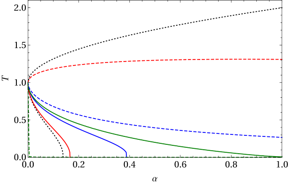
Figure 5: Critical lines for ergodicity breaking (dotted curves) and retrieval region boundary (solid curves) for various values of the unlearning time. From the top to the bottom: $t=0$ (black lines, i.e. the Hopfield phase diagram), $t=0.1$ (red lines), $1$ (blue lines) and $1000$ (green lines).

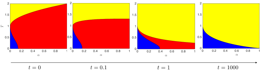
Figure 6: The phase diagram is depicted for different choices of $t$, namely, from left to right, $t=0,0.1,1,1000$. Notice that, as $t$ grows, the retrieval region (blue) and the ergodic region (yellow) get wider at the cost of the spin-glass region (red) which progressively shrinks up to collapse as $t\rightarrow\infty$. Also notice the change in the concavity of the critical line which separates ergodic and spin-glass region.

4 Conclusions and outlooks

In recent years Artificial Intelligence, mainly due to the impressive skills of Deep Learning machines and the GPU-related revolution DL1 , has attracted the attention of the whole Scientific Community. In particular, the latter includes mathematicians involved in the statistical mechanics of complex systems which has proved to be a fruitful tool in the investigation of neural networks and machine learning, since the early days (not by chance Boltzmann machines are named after Boltzmann BM1 ).
Among the various fields of Artificial Intelligence where, in the present years, statistical mechanics extensively contributed to the cause (e.g. statistical inference and signal processing Simona ; Lenka1 , combinatorial and computational complexity Lenka2 ; Zecchina ; Monasson , supervised or unsupervised learning Zecchina2 ; Huang , deep learning Chiara ; Metha , compositional capabilities Agliari-PRL1 ; Monasson2 , and really much more…) the one we deepened in this work deals with the phenomenon of dreaming and sleeping.
In the current work we mathematically described the phenomena of reinforcement and remotion, as pioneered by Crick $\&$ Mitchinson Crick , by Hopfield HopfieldUnlearning and by many others in the neuroscience literature, see e.g Neuro-1 ; Neuro0 ; Neuro1 ; Neuro2 ): interestingly, such mechanisms have been evidenced to lead to an improvement of the retrieval capacity of the system. In particular, in Albert2 , we showed that the system reaches the expected upper critical capacity $\alpha_{c}=1$, still preserving robustness with respect to fast noise. However, the statistical mechanical analysis, set at the standard replica symmetric level of description, was carried out via non-rigorous approaches (e.g., replica trick and numerical simulations).
In this work we extended a Guerra’s interpolation scheme Barra-JSP2010 , originally developed to deal with the standard Hopfield model (i.e. equipped with the canonical Hebbian synaptic coupling), to deal with this generalization: at first we showed the equivalence of this model with a three-layer spin-glass where some links among different layers are cloned (hence introducing correlation in the network and in the random fields required for the interpolation) and the third, and novel (w.r.t. the standard equivalence between Hopfield models and two-layers Boltzmann machines BarraEquivalenceRBMeAHN ; Barra-RBMsPriors2 ), layer is equipped with imaginary real-valued neurons (best suitable to perform spectral analysis). As a consequence, the resulting interpolating architecture is rather tricky, by far richer than its classical limit yet it turns out to be managable and actually a sum rule for the quenched free energy related to the model can be written and even integrated, under the assumption of replica symmetry: such an expression, as well as those stemming from its extremization for the order parameters, sharply coincides with previous results Albert2 , confirming them in each detail.
We remark that such theorems state also the validity of other previous investigation -all replica trick derived- on unlearning in neural networks (see e.g. Dotsenko1 ; unlearning1 ; KanterSompo ).
Beyond confirming previous results, we further systematically developed a fluctuation analysis of the overlap correlation functions, searching for critical behaviour, in order to inspect where ergodicity breaks down and in this investigation we found a very interesting result: as long as the Hopfield model is awake, the critical line is the one predicted by Amit-Gutfreund-Sompolinksy (as it should and as it is known by decades). However, as the network sleeps, the ergodic region starts to invade the spin glass region, ultimately destroying the spin glass states entirely, thus allowing the network (at the end of an entire sleep session) to live solely within a -quite large- retrieval region, surrounded by ergodicity: noticing that at this final stage of sleeping the network approached the Kanter-Sompolinsky model KanterSompo , it shines why these Authors called their model associative recall of memory without errors.

References

- (1) D.H. Ackley, G.E. Hinton, T.J. Sejnowski, A learning algorithm for Boltzmann machines, Cognitive Sci. 9.1:147-169, (1985).
- (2) E. Agliari, et al., Multitasking associative networks, Phys. Rev. Lett. 109, 268101, (2012).
- (3) E. Agliari, A. Barra, C. Longo, D. Tantari, Neural Networks retrieving binary patterns in a sea of real ones, J. Stat. Phys. 168, 1085, (2017).
- (4) E. Agliari, A. Barra, B. Tirozzi, Free energies of Boltzmann Machines: self-averaging, annealed and replica symmetric approximations in the thermodynamic limit, J. Stat., in press.
- (5) E. Agliari, et al., Multitasking attractor networks with neuronal threshold noises, Neural Networks 49, 19, (2013).
- (6) E. Agliari, et al., Parallel retrieval of correlated patterns: From Hopfield networks to Boltzmann machines, Neural Networks 38, 52, (2013).
- (7) E. Agliari, et al, Immune networks: multitasking capabilities near saturation, J.Phys.A: Math. Theor. 46(41):415003, (2003).
- (8) M. Aizenman, P. Contucci, On the stability of the quenched state in mean-field spin-glass models, J. Stat. Phys. 92(5-6):765, (1998).
- (9) D.J. Amit, Modeling brain functions, Cambridge Univ. Press (1989).
- (10) D. Amit, H. Gutfreund, H. Sompolinsky, Spin-glass models of neural networks, Phys. Rev. A 32.2:1007, (1985).
- (11) D. Amit, H. Gutfreund, H. Sompolinsky, Storing infinite numbers of patterns in a spin-glass model of neural networks, Phys. Rev. Lett. 55.14:1530, (1985).
- (12) A. Engel, C. Van den Broeck, Statistical mechanics of learning, Cambridge University Press (2001).
- (13) C. Baldassi, A. Braunstein, N. Brunel, and R. Zecchina, Efficient supervised learning in networks with binary synapses, Proc. Natl. Acad. Sci. 104, 11079, (2007).
- (14) M. Baity-Jesi, et al., Comparing dynamics: Deep neural networks versus glassy systems, preprint arXiv:1803.06969, (2018).
- (15) A. Barra, M. Beccaria, A. Fachechi,A new mechanical approach to handle generalized Hopfield neural networks, Neural Networks (2018).
- (16) A. Barra, et al., On the equivalence among Hopfield neural networks and restricted Boltzman machines, Neural Networks 34, 1-9, (2012).
- (17) A. Barra, et al., Phase transitions of Restricted Boltzmann Machines with generic priors, Phys. Rev. E 96, 042156, (2017).
- (18) A. Barra, et al., Phase Diagram of Restricted Boltzmann Machines Generalized Hopfield Models, Phys. Rev. E 97, 022310, (2018).
- (19) A. Barra, G. Genovese, F. Guerra, The replica symmetric approximation of the analogical neural network, J. Stat. Phys. 140(4):784, (2010).
- (20) A. Barra, G. Genovese, F. Guerra, Equilibrium statistical mechanics of bipartite spin systems, J. Phys. A 44, 245002, (2011).
- (21) A. Barra, F. Guerra, About the ergodic regime of the analogical Hopfield neural network, J. Math. Phys. 49, 125217, (2008)
- (22) A. Bovier, V. Gayrard, Hopfield models as generalized random mean field models, Mathematical aspects of spin glasses and neural networks, 3-89, Birkhauser, Boston (1998).
- (23) A. Bovier, V. Gayrard, P. Picco, Gibbs states of the Hopfield model in the regime of perfect memory, Prob. Theor. Rel. Fields 100(3):329, (1994).
- (24) A. Bovier, V. Gayrard, P. Picco, Gibbs states of the Hopfield model with extensively many patterns, J. Stat. Phys. 79(1-2):395, (1995).
- (25) P. Carmona, Y. Hu, Universality in Sherrington–Kirkpatrick’s spin glass model, Ann. Henri Poincarè 42, 2, (2006).
- (26) S. Cocco, R. Monasson, Adaptive cluster expansion for inferring Boltzmann machines with noisy data, Phys. Rev. Lett. 106.9: 090601, (2011).
- (27) A.C.C. Coolen, R. Kuhn, P. Sollich, Theory of neural information processing systems, Oxford Press (2005).
- (28) P. Contucci, C. Giardinà, Spin-Glass Stochastic Stability: a Rigorous Proof, Annales Henri Poincaré 6:915-923, (2005).
- (29) F. Crick, G. Mitchinson, The function of dream sleep, Nature 304, 111, (1983).
- (30) S. Diekelmann, J. Born, The memory function of sleep, Nature Rev. Neuroscience 11(2):114, (2010).
- (31) V. Dotsenko, N.D. Yarunin, E.A. Dorotheyev, Statistical mechanics of Hopfield-like neural networks with modified interactions, J. Phys. A 24, 2419, (1991).
- (32) V. Dotsenko, B. Tirozzi, Replica symmetry breaking in neural networks with modified pseudo-inverse interactions, J. Phys. A 24:5163-5180, (1991).
- (33) A. Fachechi, E. Agliari, A. Barra, Dreaming neural networks: forgetting spurious memories and reinforcing pure ones, submitted to Neural Nets available at arXiv:1810.12217 (2018).
- (34) E. Gardner, The space of interactions in neural network models, J. Phys. A 21(1):257, (1988).
- (35) G. Genovese, Universality in bipartite mean field spin glasses, J. Math. Phys. 53(12):123304, (2012).
- (36) I. Goodfellow, Y. Bengio, A. Courville, Deep Learning, M.I.T. press (2017).
- (37) A. Hern, Yes, androids do dream of electric sheep, The Guardian, Technology and Artificial Intelligence (2015).
- (38) J.A. Hobson, E.F. Pace-Scott, R. Stickgold, Dreaming and the brain: Toward a cognitive neuroscience of conscious states, Behavioral and Brain Sciences 23, (2000).
- (39) J.J. Hopfield, Neural networks and physical systems with emergent collective computational abilities, Proceedings of the national academy of sciences 79.8 (1982): 2554-2558.
- (40) J.J. Hopfield, D.I. Feinstein, R.G. Palmer, Unlearning has a stabilizing effect in collective memories, Nature Lett. 304, 280158, (1983).
- (41) J.A. Horas, P.M. Pasinetti, On the unlearning procedure yielding a high-performance associative memory neural network, J. Phys. A 31, L463-L471, (1998).
- (42) H. Huang, K. Y. Michael Wong, and Y. Kabashima, Entropy landscape of solutions in the binary perceptron problem, J. Phys. A 46, 375002, (2013).
- (43) I. Kanter, H. Sompolinsky, Associative recall of memory without errors, Phys. Rev. A 35.1:380, (1987).
- (44) F. Krzakala, M. Mezard, F. Sausset, Y.F. Sun, L. Zdeborova, Statistical-physics-based reconstruction in compressed sensing, Phys. Rev. X 2(2), 021005, (2012).
- (45) F. Krzakała, A. Montanari, F. Ricci-Tersenghi, G. Semerjian, L. Zdeborova, Gibbs states and the set of solutions of random constraint satisfaction problems, Proc. Natl. Acad. Sci. 104:(25),10318, (2007).
- (46) Y. Le Cun, Y. Bengio, G. Hinton, Deep learning, Nature 521:436-444, (2015).
- (47) P. Maquet, The role of sleep in learning and memory, Science 294.5544:1048, (2001).
- (48) J.L. McGaugh, Memory - a century of consolidation, Science 287.5451:248-251, (2000).
- (49) M. Mezard, G. Parisi, M.A. Virasoro, Spin glass theory and beyond: an introduction to the replica method and its applications, World Scientific, Singapore (1987)
- (50) M. Mezard, G. Parisi, R. Zecchina, Analytic and algorithmic solution of random satisfiability problems, Science 297.5582:812-815, (2002).
- (51) P. Mehta, D.J. Schwab, An exact mapping between the variational renormalization group and deep learning, preprint, arXiv:1410.3831, (2014).
- (52) R. Monasson, R. Zecchina, S. Kirkpatrick, B. Selman, L. Troyansky, Determining computational complexity from characteristic phase transitions, Nature 400(6740), 133, (1999).
- (53) K. Nokura, Spin glass states of the anti-Hopfield model, J. Phys. A 31, 7447, (1998).
- (54) K. Nokura, Paramagnetic unlearning in neural network models, Phys. Rev. E 54(5):5571, (1996).
- (55) L. Pastur, M. Shcherbina, B. Tirozzi, The replica-symmetric solution without replica trick for the Hopfield model, J. Stat. Phys. 74(5-6):1161, (1994).
- (56) L. Pastur, M. Shcherbina, B. Tirozzi, On the replica symmetric equations for the Hopfield model, J. Math. Phys. 40(8): 3930, (1999).
- (57) L. Personnaz, I. Guyon, G. Dreyfus, Information storage and retrieval in spin-glass like neural networks, J. Phys. Lett. 46, L-359:365, (1985).
- (58) R. Salakhutdinov, G. Hinton, Deep Boltzmann machines, Artificial Intelligence and Statistics (2009).
- (59) R. Salakhutdinov, H. Larochelle, Efficient learning of deep Boltzmann machines, Proc. thirteenth int. conf. on artificial intelligence and statistics, 693, 2010.
- (60) H.S. Seung, H. Sompolinsky, N. Tishby, Statistical mechanics of learning from examples, Phys. Rev. A 45(8):6056, (1992).
- (61) M. Talagrand, Rigorous results for the Hopfield model with many patterns, Prob. Theor. Rel. Fiel. 110(2):177, (1998).
- (62) M. Talagrand, Exponential inequalities and convergence of moments in the replica-symmetric regime of the Hopfield model, Ann. Prob. 1393-1469, (2000).
- (63) J. Tubiana, R. Monasson, Emergence of Compositional Representations in Restricted Boltzmann Machines, Phys. Rev. Lett. 118.13:138301, (2017).
- (64) S. Wimbauer, J. Leo van Hemmen, Hebbian unlearning, Analysis of Dynamical and Cognitive Systems, Springer, Berlin, 1995.