We show how theoretical uncertainties due to nuclear effects may be incorporated into global fits of proton parton distribution functions (PDFs) that include deep-inelastic scattering and Drell-Yan data on nuclear targets. We specifically consider the CHORUS, NuTeV and E605 data included in the NNPDF3.1 fit, which used Pb, Fe and Cu targets, respectively. We show that the additional uncertainty in the proton PDFs due to nuclear effects is small, as expected, and in particular that the effect on the $\bar{d}/\bar{u}$ ratio, the total strangeness $s+\bar{s}$, and the strange valence distribution $s-\bar{s}$ is negligible.

1 Introduction

Modern sets of parton distribution functions (PDFs) [1] are currently determined for the proton from a global quantum chromodynamics (QCD) analysis of hard-scattering measurements [2]. A variety of hadronic observables are used, including some from processes that do not (exclusively) involve protons in the initial state, such as deep-inelastic scattering (DIS) and Drell-Yan (DY) in experiments with deuterium or heavy nuclear fixed targets. These experiments complement the proton-only ones, providing important sensitivity to light PDF flavour separation [3], and are therefore included in most contemporary global QCD analyses.

The inclusion of nuclear data necessitates accounting for differences between the PDFs for free nucleons and those for partons contained within nuclei. In the past a variety of different approaches have been adopted: nuclear corrections can be ignored on the basis that they are small [3], included according to various nuclear models [4, 5, 6], or determined in a fit to the data [7]. Whatever approach is adopted, nuclear effects will necessarily increase the uncertainty in the proton PDFs, since nuclear corrections are not known very precisely. So far the size of this uncertainty has also been regarded as small [8, 9]. However, in recent years the inclusion of increasingly precise LHC measurements in global PDF fits has reduced PDF uncertainties to the level of a few percent [3]. Furthermore, nuclear effects have been claimed to alter the shape of the PDFs, especially at large values of the momentum fraction $x$ [10], albeit without an estimate of the corresponding theoretical uncertainty. Given this, it is becoming increasingly desirable to provide PDF sets that include such an uncertainty.

In this paper we will show how this may be achieved by performing global fits which include nuclear uncertainties, in the framework of the NNPDF3.1 global analysis [3]. We focus on the DIS and DY datasets with heavy nuclear targets (Pb, Fe and Cu). We estimate the theoretical uncertainty due to neglecting the corresponding nuclear corrections, we include it in a fit along with the experimental uncertainty, and we assess its impact on the resulting PDFs. A similar exercise for DIS and DY datasets with deuterium targets will be carried out in a separate analysis.

Our study is accomplished within the formalism of Ref. [11], that was developed to include a broad class of theoretical uncertainties in a PDF fit. The method consists of adding to the experimental covariance matrix a theoretical covariance matrix, estimated in the space of the data according to the theoretical uncertainties associated with the theoretical predictions. In practice this means that the theoretical uncertainties are treated in much the same way as experimental systematics. Here we will estimate the theoretical uncertainties associated with nuclear effects. This will be done empirically, by directly comparing theoretical predictions computed using nuclear PDFs (nPDFs) to those computed using proton PDFs. This comparison will allow us to construct the covariance matrix associated with the nuclear effects, and thus incorporate these effects in a global proton PDF fit. The fitting methodology will otherwise be the same as in the NNPDF3.1 analysis, allowing for a direct comparison of the results.

The paper is organised as follows. In Sect. 2, we summarise the changes in methodology required to include theoretical uncertainties in a global fit. We then describe the nuclear dataset included in this analysis, emphasising to which PDF flavours it is most sensitive. We next provide two alternative prescriptions to estimate the theoretical covariance matrix, and discuss their implementation. In Sect. 3, we present the impact of nuclear data and theoretical corrections in a global fit of PDFs. We compare variants of the NNPDF3.1 determination obtained by removing the nuclear datasets completely, or by retaining them but accounting for nuclear uncertainties, and nuclear corrections. We study the fit quality and the stability of the PDFs. Given that the nuclear dataset is mostly sensitive to sea quark PDFs, in Sect. 4 we assess how the $\bar{d}$-$\bar{u}$ asymmetry, and the strangeness content of the proton, including the asymmetry between $s$ and $\bar{s}$ PDFs, are affected by nuclear uncertainties. We provide our conclusions and an outlook in Sect. 5.

2 Theoretical Uncertainties due to Nuclear Corrections

In this section we describe how the NNPDF methodology can be adapted to incorporate theoretical uncertainties through a theoretical covariance matrix, as proposed in Ref. [11]. We then focus on the DIS and DY datasets in the NNPDF3.1 global dataset (described in detail in Sect. 2 of Ref. [3]) that involve nuclear targets other than deuterium. We first summarise the type of measured observables, their kinematic coverage, and their sensitivity to the underlying PDFs. We then show how the size of the nuclear effects may be estimated empirically by comparing the different theoretical predictions made with proton and nuclear PDFs. We finally offer two alternative prescriptions to estimate the theoretical covariance matrix for the nuclear uncertainties: the first of which simply provides a conservative estimate of the overall uncertainty; the second of which also applies a correction for nuclear effects, aiming to reduce the overall uncertainty.

2.1 Theoretical Uncertainties in PDF Fits

The NNPDF fitting methodology [12] works in two stages. We start from a set of experimental data points $D_{i}$, $i=1,\ldots,N_{\rm dat}$, with an associated experimental covariance matrix $C_{ij}$ (which includes all experimental statistical and systematic uncertainties). We then generate data replicas $D_{i}^{(k)}$, $k=1,\ldots,N_{\rm rep}$, which are Gaussianly distributed in such a way that their ensemble averages reproduce the data and their uncertainties:

$$\langle D_{i}^{(k)}\rangle=D_{i},\qquad\langle(D_{i}^{(k)}-D_{i})(D_{j}^{(k)}-D_{j})\rangle=C_{ij}\,,$$ (1)

where the ensemble average $\langle\cdot\rangle$ is taken over a sufficiently large ensemble of data replicas (in principle strict equality only holds in the limit $N_{\rm rep}\to\infty$).

We then compare theoretical predictions $T_{i}[f]$, which depend on the PDFs $f$ (or more precisely the neural network parameters which parametrise these PDFs), to the data replicas, by optimising a figure of merit:

$$\chi^{2}[f,D]=\frac{1}{N_{\rm dat}}\sum_{i,j}(T_{i}[f]-D_{i})\,(C_{0}^{-1})_{ij}\,(T_{j}[f]-D_{j})\,.$$ (2)

Here, $C_{0}$ is the $t_{0}$-covariance matrix used in the fit. If all the experimental uncertainties were additive, $(C_{0})_{ij}$ would simply be the experimental covariance matrix $C_{ij}$, but in the presence of multiplicative uncertainties this would bias the fit [13]. To eliminate this bias we use instead $(C_{0})_{ij}$, constructed from $C_{ij}$ using the $t_{0}$ method [14]. The method requires the PDF dependence implicit in $(C_{0})_{ij}$ to be iterated to consistency; in practice this iteration converges very rapidly, as the dependence is very weak.

In this way we obtain a PDF replica $f^{(k)}$ for each data replica $D^{(k)}$. Since the distribution of the PDF replicas is a representation of the distribution of the data replicas, the ensemble of PDF replicas $\{f^{(k)}\}$ gives us a representation of the PDFs and their correlated uncertainties.

We can incorporate theory uncertainties into the NNPDF methodology by supplementing the experimental covariance matrix $C_{ij}$ with a theoretical covariance matrix $S_{ij}$, estimated using the theoretical uncertainties associated with the theoretical predictions $T_{i}[f]$. The experimental and theoretical uncertainties are by their nature independent. In Ref.[11] it was shown that if we assume that both experimental and theoretical uncertainties are independent and Gaussian, the two covariance matrices can simply be added; the combined covariance matrix $C_{ij}+S_{ij}$ then gives the total uncertainty in the extraction of PDFs from the experimental data.

In practice this means that, when we generate the data replicas, in place of Eq. (1) we need

$$\langle D_{i}^{(k)}\rangle=D_{i},\qquad\langle(D_{i}^{(k)}-D_{i})(D_{j}^{(k)}-D_{j})\rangle=C_{ij}+S_{ij},$$ (3)

to ensure that the theoretical uncertainty is propagated through to the PDFs along with the experimental uncertainties. Likewise when we fit, in place of Eq.(2) we use as the figure of merit

$$\chi^{2}[f,D]=\frac{1}{N_{\rm dat}}\sum_{i,j}(T_{i}[f]-D_{i})\,(C_{0}+S)^{-1}_{ij}\,(T_{j}[f]-D_{j})\,.$$ (4)

This ensures that the fitting accounts for the relative weight of the data points according to both the experimental and the theoretical uncertainties.

It remains to estimate the theoretical covariance matrix $S_{ij}$. In general this will be constructed in the same way as an experimental systematic: a range of theoretical predictions $T_{i}^{(n)}$ can be characterised by nuisance parameters, $\Delta_{i}^{(n)}=T_{i}^{(n)}-T_{i}$, $n=1,\ldots,N_{\rm nuis}$. Assuming that we can model the theoretical uncertainties by a Gaussian characterised by these nuisance parameters, we can write

$$S_{ij}=\mathcal{N}\sum_{n=1}^{N_{\rm nuis}}\Delta^{(n)}_{i}\Delta^{(n)}_{j}\,,$$ (5)

where ${\cal N}$ is a normalisation which depends on whether the nuisance parameters are independent uncertainties, or different estimates of the same uncertainty.

Note that since the predictions $T_{i}[f]$ depend on the PDFs, this means the nuisance parameters $\Delta_{i}^{(n)}$ and the theoretical covariance matrix $S_{ij}$ will also depend implicitly on the PDF, albeit weakly. This can be dealt with in precisely the same way as in the $t_{0}$ method [14]: $S_{ij}$ is computed with an initial (central) PDF, which is then iterated to consistency. In practice the iterations can be performed simultaneously.

In this paper we will show how this procedure works by estimating the theoretical uncertainties due specifically to nuclear effects related to the use of data from scattering off heavy nuclear targets.

2.2 The Nuclear Dataset

The NNPDF3.1 dataset involving heavy nuclei consists of inclusive charged-current DIS cross sections from CHORUS [15], DIS dimuon cross sections from NuTeV [16, 17], and DY dimuon cross sections from E605 [18]. In the case of CHORUS and NuTeV, neutrino and antineutrino beams are scattered off a lead (${}^{208}_{\ 82}$Pb) and an iron (${}^{56}_{26}$Fe) target, respectively; while in the case of E605 a proton beam is scattered off a copper (${}^{64}_{32}$Cu) target. Henceforth we refer to the combined measurements from CHORUS, NuTeV and E605 as the nuclear dataset. In NNPDF3.1 there are additional DIS and DY datasets involving scattering from deuterium: nuclear corrections to these datasets will be considered in a future analysis. In NNPDF we do not use the CDHSW neutrino-DIS data [19], taken with an iron target.

An overview of the nuclear dataset is presented in Table 1, where we indicate, for each dataset: the observable, the corresponding reference, the number of data points before and after kinematic cuts, and the kinematic range covered in the relevant variables after cuts. Kinematic cuts match the next-to-next-to-leading order (NNLO) NNPDF3.1 baseline fit: for DIS we require $Q^{2}\geq 3.5$ GeV² and $W^{2}\geq 12.5$ GeV², where $Q^{2}$ and $W^{2}$ are the energy transfer and the invariant mass of the final state in the DIS process, respectively; for DY, we require $\tau\leq 0.080$ and $|y_{\ell\ell}/y_{\rm max}|\leq 0.663$, where $\tau=M_{\ell\ell}^{2}/s$ and $y_{\rm max}=-\frac{1}{2}\ln\tau$, with $y_{\ell\ell}$ and $M_{\ell\ell}$ the rapidity and the invariant mass of the dimuon pair, respectively, and $\sqrt{s}$ the centre-of-mass energy of the DY process.

The kinematic coverage of the three experiments in the $(x,Q^{2})$ plane is compared to the whole of the NNPDF3.1 dataset in Fig. 1, where points corresponding to the nuclear dataset are circled in black. For hadronic data, the momentum fraction $x$ has been reconstructed from leading-order (LO) kinematics (using central rapidity for those observables integrated over rapidity), and the value of $Q^{2}$ has been set equal to the characteristic scale of the process. The number of data points after cuts is $4285$, out of which $993$ belong to the nuclear dataset (corresponding to about $23\%$ of the entire dataset). Most of the nuclear data (around $84\%$) are from CHORUS.

Experiment	Obs.	Ref.	$N_{\rm dat}$		${\rm Kin}_{1}$	${\rm Kin}_{2}$ [GeV]
CHORUS	$\sigma^{\nu}$	[15]	607	(416)	$0.045\leq x\leq 0.65$	$1.9\leq Q\leq 9.8$
	$\sigma^{\bar{\nu}}$	[15]	607	(416)	$0.045\leq x\leq 0.65$	$1.9\leq Q\leq 9.8$
NuTeV	$\sigma^{\nu,c}$	[16, 17]	45	(39)	$0.02\leq x\leq 0.33$	$2.0\leq Q\leq 10.8$
	$\sigma^{\bar{\nu},c}$	[16, 17]	45	(37)	$0.02\leq x\leq 0.21$	$1.9\leq Q\leq\ \,8.3$
E605	$\sigma_{\rm DY}^{p}$	[18]	119	(85)	$-0.2\leq y_{\ell\ell}\leq 2.9$	$7.1\leq M_{\ell\ell}\leq 10.9$

Table 1: The datasets involving nuclear targets other than deuterium in NNPDF3.1. The kinematic range covered in each variable is given after cuts are applied (see the text for details).

Figure 1: The kinematic coverage of the current analysis, equivalent to that of the NNPDF3.1 analysis, in the $(x,Q^{2})$ plane. Points belonging to the nuclear dataset are circled in black.

The observables measured by CHORUS, NuTeV and E605 allow one to control the valence-sea (or quark-antiquark) separation at medium-to-high values of the momentum fraction $x$, and at a rather low energy $Q^{2}$. Following their factorised form, charged current DIS cross sections measured by CHORUS are expected to provide some information on the valence distributions $u_{V}=u-\bar{u}$ and $d_{V}=d-\bar{d}$; DIS dimuon cross sections, reconstructed by NuTeV from the decay of a charm quark, are sensitive to $s$ and $\bar{s}$ PDFs; and DY dimuon cross sections measured by E605 probe $\bar{u}$ and $\bar{d}$ PDFs.

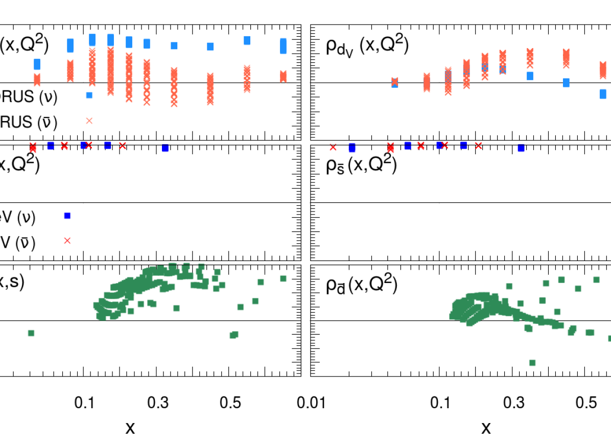
Figure 2: The correlation coefficient $\rho$ between the observables in Table 1 and (from top to bottom) the $u_{V}$ and $d_{V}$ PDFs for CHORUS, the $s$ and $\bar{s}$ PDFs for NuTeV, and the $\bar{u}$ and $\bar{d}$ PDFs for E605.

The sensitivity of the measured observables to different PDF flavours can be quantified by the correlation coefficient $\rho$ (defined in Eq. (1) in Ref. [20]) between the PDFs in a given set and the theoretical predictions corresponding to the measured data points. Large values of $|\rho|$ indicate that the sensitivity of the PDFs to the data is most significant. The correlation coefficient $\rho$ is displayed in Fig 2, from top to bottom, for the $u_{V}$ and $d_{V}$ PDFs from CHORUS, for the $s$ and $\bar{s}$ PDFs from NuTeV, and for the $\bar{u}$ and $\bar{d}$ PDFs from E605. Each point corresponds to a different datum in the experiments enumerated in Table 1: PDFs are taken from the NNDPF3.1 NNLO parton set, and are evaluated at a scale equal to either the momentum transfer $Q^{2}$ (for DIS) or the center-of-mass energy $s$ (for DY) of that point. For DY, the value of $x$ is computed from hadronic variables using LO kinematics. As anticipated, the correlation between the PDF flavours and the observables displayed in Fig. 2 is sizeable, in particular: between $u_{V}$ ($d_{V}$) PDFs and the neutrino (antineutrino) charged current DIS cross sections from CHORUS in the range $0.1\leq x\leq 0.7$ ($0.2\leq x\leq 0.5$); between $s$ ($\bar{s}$) PDFs and the antineutrino dimuon DIS cross sections from NuTeV along all the measured range, $0.02\leq x\leq 0.32$ ($0.02\leq x\leq 0.21$); and between $\bar{u}$ ($\bar{d}$) PDFs and the dimuon DY cross sections from E605 in the range $0.3\leq x\leq 0.7$. Correlations between the measured observables and other PDFs, not displayed in Fig. 2, are relatively small. We therefore expect that including theoretical uncertainties due to nuclear corrections will mainly affect the valence-sea PDF flavour separation in the kinematic region outlined above.

2.3 Determining Correlated Nuclear Uncertainties

In Sec. 2.1, we explained how, if we want to include theoretical uncertainties in a PDF fit, we first need to estimate the theoretical covariance matrix $S_{ij}$ in the space of the data, using Eq. (5). In this section, we illustrate how we might achieve this for the nuclear uncertainties affecting the three datasets described in Sec. 2.2. First we provide two alternative definitions for the theoretical covariance matrix associated with nuclear uncertainties, then we describe how we can implement them in practice, and finally we discuss the results.

2.3.1 Definition

We construct the point-by-point correlated elements $S_{ij}$ of the theoretical covariance matrix as the unweighted average over $N_{\rm nuis}$ nuisance parameters $\Delta_{i,j}^{(n)}$ for each data point $i,j=1,\dots,N_{\rm dat}$, as in Eq. (5). A conservative definition of the nuisance parameters for nuclear uncertainties, which takes into account all the uncertainty due to the difference between nuclear and proton targets, is

$$\Delta_{i}^{(n)}=T^{N}_{i}[f_{N}^{(n)}]-T^{N}_{i}[f_{p}]\,,$$ (6)

where $T^{N}_{i}[f_{N}^{(n)}]$ and $T^{N}_{i}[f_{p}]$ denote the theoretical prediction for the nuclear observable using a PDF $f_{N}^{(n)}$ for a heavy nucleus $N$, and the corresponding prediction using a proton PDF $f_{p}$. The subscript $N$ identifies the appropriate isotope, i.e. $N={{}^{208}_{\ 82}{\rm Pb}}$ for CHORUS, $N={{}^{56}_{26}{\rm Fe}}$ for NuTeV, and $N={{}^{64}_{32}{\rm Cu}}$ for E605. The superscript $n$ identifies a particular model of nuclear corrections.

Various models of nuclear effects on PDFs exist in the literature (for a review, see, e.g., Ref. [21]). They are however based on a range of different assumptions, which often limit their validity. In our opinion, a better ansatz for nuclear effects, over all the kinematic range covered by the measurements in Table 1, is provided by global fits of nPDFs, since they are primarily driven by the data. The $N_{\rm nuis}$ models in Eq. (5) can then be identified with different members of a nPDF set. The free proton PDF can instead be taken from a global set of proton PDFs: it should in any case be iterated to consistency at the end of the fitting procedure, as explained at the end of Sec.2.1. The practical way in which nPDF members are constructed, the proton PDF is chosen, and the corresponding observables are computed is discussed in Sect. 2.3.2 below.

A more ambitious definition of the nuisance parameters $\Delta_{i}^{(n)}$ in Eq. (5) is to consider the theoretical uncertainty to be due only to the uncertainties in the nPDFs themselves. Therefore

$$\Delta_{i}^{(n)}=T^{N}_{i}[f_{N}^{(n)}]-T^{N}_{i}[f_{N}]\,,$$ (7)

where, in comparison to Eq. (6), the expectation value of the proton observable is now replaced by the central value of the nPDFs $f_{N}=\langle f_{N}^{(n)}\rangle$. Because Eq. (7) does not contain any information on how nuclear observables differ from the corresponding proton ones, Eq. (7) must be supplemented with a shift, applied to each data point $i$, that takes into account the difference between the two:

$$\delta T^{N}_{i}=T^{N}_{i}[f_{N}]-T^{N}_{i}[f_{p}].$$ (8)

This can be thought of as the nuclear correction to the theoretical predictions, which is equivalent to a correction to the data, when used in Eq. (4).

The two definitions are in principle different. In Eq. (6), the contribution of the nuclear data to the global fit is deweighted by an extra uncertainty, which encompasses both the difference between the proton and nuclear PDFs, and the uncertainty in the nPDFs. In Eqs. (8) the theory is corrected by a shift. Here the uncertainty, and thus the deweighting, is correspondingly smaller, arising only from the uncertainty in the nPDFs. In principle, if the uncertainty in the nPDFs is correctly estimated, and smaller than the shift, the second definition should give more precise results. However if the shift is small, or unreliably estimated, the first definition will be better, and should result in a lower $\chi^{2}$ for the nuclear data, albeit with slightly larger PDF uncertainties.

2.3.2 Implementation

The goal of our exercise is to estimate the overall level of theoretical uncertainty associated to nuclear effects. Inconsistency (following from somewhat inconsistent parametrisations) should be part of that, therefore, instead of relying on a single nPDF determination in Eqs. (6-8), we find it useful to utilise a combination of different nPDF sets. Such a combination can be realised in a statistically sound way by following the methodology developed in Ref. [1], which consists in taking the unweighted average of the nPDF sets. The simplest way of realing it is to generate equal numbers of Monte Carlo replicas from each input nPDF set, and then merge them together in a single Monte Carlo ensemble. The appropriate normalisation in Eq. (5) is therefore ${\cal N}=\frac{1}{N_{\rm nuis}}$, since each replica is equally probable; each nPDF member in Eqs. (6-8) is a replica in the Monte Carlo ensemble; and $f_{N}=\langle f_{N}^{(n)}\rangle$ is the zero-th replica in the same Monte Carlo ensemble. The combination method of Ref. [1] has proven to be adequate when results are compatible or differences are understood, as is the case with nPDFs.

The Monte Carlo ensemble utilised to compute Eqs. (6-8) is determined as follows. We consider recent nPDF sets available in the literature, namely DSSZ12 [22], nCTEQ15 [23] and EPPS16 [24]. These are determined at next-to-leading order (NLO) from a global analysis of measurements in DIS, DY and proton-nucleus ($pN$) collisions. A compilation of the data included in these sets is given in Table 2. A detailed description may be found in Refs. [22, 23, 24], and a critical comparison is documented, e.g., in Refs. [25, 26]. As one can see, all three determinations include a significant amount of experimental information, so should collectively provide a reasonable representation of nuclear modifications.

The nuclear datasets used in NNPDF3.1, and hence in the fits performed in this analysis, also enter some of the nPDFs selected above. This is the case of NuTeV measurements (also included in DSSZ12) and of CHORUS measurements (also included in DSSZ12 and EPPS16), see Table 1 and Table 2. This does not lead to a double counting of these data because we only use the nPDFs as a model to establish an additional correlated source of uncertainty in the determination of the proton PDFs. This then leads to an increase in overall uncertainties, since the nuclear datasets are deweighted, while double counting would give a decrease in uncertainties.

However the nuclear corrections, computed in this way, implicitly assume an underlying proton PDF (this is what a fit of nPDFs does). In this respect, the process is conceptually equivalent to the inclusion of nuclear corrections in a fit of proton PDFs according to some phenomenological model whose parameters are tuned to the data beforehand, as done, for instance, in Ref. [4]. In principle, the procedure should be iterated to consistency [11]: the output of a proton PDF fit including the nuclear uncertainties can be used to update a fit of nPDFs, which can be used in turn to refine the estimate of the theoretical covariance matrix, Eq. (5), to be included in a subsequent fit of proton PDFs. In practice however this iteration is unecessary, since we will find that the effect of the nuclear correction is already very small. This is fortunate, since we are in any case not yet able to consistently perform nPDF fits within the NNPDF framework.

Observable	Experiment	Ref.	$N_{\rm dat}$ (DSSZ12)	$N_{\rm dat}$ (nCTEQ15)	$N_{\rm dat}$ (EPPS16)
$F_{2}^{\rm D}/F_{2}^{\rm D}$	NMC	[27]	—	201	—
$F_{2}^{\rm He}/F_{2}^{\rm D}$	NMC	[28]	17	12	16
	E139	[29]	18	3	21
	HERMES	[30]	—	17	—
$F_{2}^{\rm Li}/F_{2}^{\rm D}$	NMC	[31]	17	11	15
$F_{2}^{\rm Li}/F_{2}^{\rm D}$ $Q^{2}$ dep	NMC	[31]	—	—	153
$F_{2}^{\rm Be}/F_{2}^{\rm D}$	E139	[29]	17	3	20
$F_{2}^{\rm C}/F_{2}^{\rm D}$	E665	[32]	—	3	—
	E139	[29]	7	2	7
	EMC	[33]	9	9	—
	NMC	[27, 28]	17	24	31
$F_{2}^{\rm C}/F_{2}^{\rm D}$ $Q^{2}$ dep	NMC	[28]	191	—	165
$F_{2}^{\rm N}/F_{2}^{\rm D}$	HERMES	[30]	—	19	—
	BCDMS	[34]	—	9	—
$F_{2}^{\rm Al}/F_{2}^{\rm D}$	E139	[29]	17	3	20
$F_{2}^{\rm Ca}/F_{2}^{\rm D}$	NMC	[28]	16	12	15
	E665	[32]	—	3	—
	E139	[29]	7	2	7
$F_{2}^{\rm Fe}/F_{2}^{\rm D}$	E049	[35]	—	2	—
	E139	[29]	23	6	26
	BCDMS	[36, 34]	—	16	—
$F_{2}^{\rm Cu}/F_{2}^{\rm D}$	EMC	[37, 33]	19	27	19
$F_{2}^{\rm Kr}/F_{2}^{\rm D}$	HERMES	[30]	—	12	—
$F_{2}^{\rm Ag}/F_{2}^{\rm D}$	E139	[29]	7	2	7
$F_{2}^{\rm Sn}/F_{2}^{\rm D}$	EMC	[33]	8	8	—
$F_{2}^{\rm Xe}/F_{2}^{\rm D}$	E665	[32]	—	2	—
$F_{2}^{\rm Au}/F_{2}^{\rm D}$	E139	[29]	18	3	21
$F_{2}^{\rm Pb}/F_{2}^{\rm D}$	E665	[32]	—	3	—
$F_{2}^{\rm C}/F_{2}^{\rm Li}$	NMC	[28]	24	7	20
$F_{2}^{\rm Ca}/F_{2}^{\rm Li}$	NMC	[28]	24	7	20
$F_{2}^{\rm Be}/F_{2}^{\rm C}$	NMC	[38]	15	14	15
$F_{2}^{\rm Al}/F_{2}^{\rm C}$	NMC	[38]	15	14	15
$F_{2}^{\rm Ca}/F_{2}^{\rm C}$	NMC	[28]	39	21	15
$F_{2}^{\rm Fe}/F_{2}^{\rm C}$	NMC	[38]	15	14	15
$F_{2}^{\rm Sn}/F_{2}^{\rm C}$	NMC	[39]	15	—	15
$F_{2}^{\rm Sn}/F_{2}^{\rm C}$ $Q^{2}$ dep	NMC	[39]	145	111	144
$F_{2}^{\rm Pb}/F_{2}^{\rm C}$	NMC	[38]	15	14	15
$F_{2}^{\rm\nu Fe}$	NuTeV	[40]	75	—	—
	CDHSW	[19]	120	—	—
$F_{3}^{\rm\nu Fe}$	NuTeV	[40]	75	—	—
	CDHSW	[19]	133	—	—
$F_{2}^{\rm\nu Pb}$	CHORUS	[15]	63	—	412
$F_{3}^{\rm\nu Pb}$	CHORUS	[15]	63	—	412
$\sigma_{\rm DY}^{\rm pC}/\sigma_{\rm DY}^{\rm pD}$	E772	[41]	9	9	9
$\sigma_{\rm DY}^{\rm pCa}/\sigma_{\rm DY}^{\rm pD}$	E772	[41]	9	9	9
$\sigma_{\rm DY}^{\rm pFe}/\sigma_{\rm DY}^{\rm pD}$	E772	[41]	9	9	9
$\sigma_{\rm DY}^{\rm pW}/\sigma_{\rm DY}^{\rm pD}$	E772	[41]	9	9	9
$\sigma_{\rm DY}^{\rm pFe}/\sigma_{\rm DY}^{\rm pBe}$	E886	[42]	28	28	28
$\sigma_{\rm DY}^{\rm pW}/\sigma_{\rm DY}^{\rm pBe}$	E886	[42]	28	28	28
$d\sigma_{\pi^{0}}^{\rm dAu}/d\sigma_{\pi^{0}}^{pp}$	PHENIX	[43]	21	20	20
	STAR	[44]	—	12	—
$d\sigma_{\pi^{-}}^{\rm pW}/d\sigma_{\pi^{-}}^{pD}$	NA10	[45]	—	—	10
$d\sigma_{\pi^{+}}^{\rm pW}/d\sigma_{\pi^{-}}^{pW}$	E615	[46]	—	—	11
$d\sigma_{\pi^{-}}^{\rm pPt}/d\sigma_{\pi^{-}}^{pH}$	NA3	[47]	—	—	7
$W^{\rm\pm}$ pPb	CMS	[48]	—	—	10
$Z$ pPb	CMS	[49]	—	—	6
	ATLAS	[50]	—	—	7
dijet pPb	CMS	[51]	—	—	7
			1579	1627	1811

Table 2: The DIS, DY and $pp$ data entering the nPDF sets used in this analysis.

The three nPDF sets selected above are each delivered as Hessian sets, corresponding to 90% confidence levels (CLs) for nCTEQ15 and EPPS16. These CLs were determined by requiring a tolerance $T=\sqrt{\Delta\chi^{2}}$, with $\Delta\chi^{2}=35$, and $\Delta\chi^{2}=52$, for the two nPDF sets, respectively. Excursions of the individual eigenvector directions resulting in a $\Delta\chi^{2}$ up to 30 units, which correspond to an increase in $\chi^{2}$ of about $2\%$, are tolerated in DSSZ12. We assume that this represents the $68\%$ CL of the fit [52]. To generate corresponding Monte Carlo sets, we utilise the Thorne-Watt algorithm [53] implemented in the public code of Ref. [54], and rescale all uncertainties to 68% CLs. We then generate $300$ replicas for each nPDF set. The size of the Monte Carlo ensemble is chosen to reproduce the central value and the uncertainty of the original Hessian sets with an accuracy of few percent. Such an accuracy is smaller than the spread of the nPDF sets, and therefore adequate for our purpose. We assume that all the three nPDF Monte Carlo sets are equally likely representations of the same underlying probability distribution, and we combine them by choosing equal numbers of replicas from each set. In the case of CHORUS and NuTeV, both lead and iron nPDFs are available from DSSZ12, nCTEQ15, and EPPS16, therefore the total number of replicas in the combined set is $N_{\rm nuis}=900$; in the case of E605, copper nPDFs are only available from nCTEQ15 and EPPS16, therefore for E605 $N_{\rm nuis}=600$. In principle, the large number of Monte Carlo replicas (and nuisance parameters) can be reduced by means of a suitable compression algorithm [55] without a significant statistical loss. A Monte Carlo ensemble of approximately the typical size of the starting Hessian sets could thus be obtained. However, we do not find it necessary to do this in the current analysis.

We then use this Monte Carlo ensemble of nPDFs, $\{\tilde{f}_{p/N}^{(n)}\}$, to determine the nuclear correction factors

$$R_{f}^{N,(n)}=\frac{\tilde{f}_{p/N}^{(n)}}{\tilde{f}_{p}}\,,$$ (9)

where $\tilde{f}_{p/N}^{(n)}$ is the bound-proton replica and $\tilde{f}_{p}$ is the central value of the free-proton PDF originally used in the corresponding nPDF analysis (namely CT14 [5] for EPPS16, a variation of the CTEQ6.1 analysis presented in Ref. [56] for nCTEQ15, and MSTW08 [57] for DSSZ12). The ratio Eq. (9) is relatively free from systematic uncertainties, and in particular has only a weak dependence on the input PDF $\tilde{f}_{p}$, as most dependence cancels in the ratio.

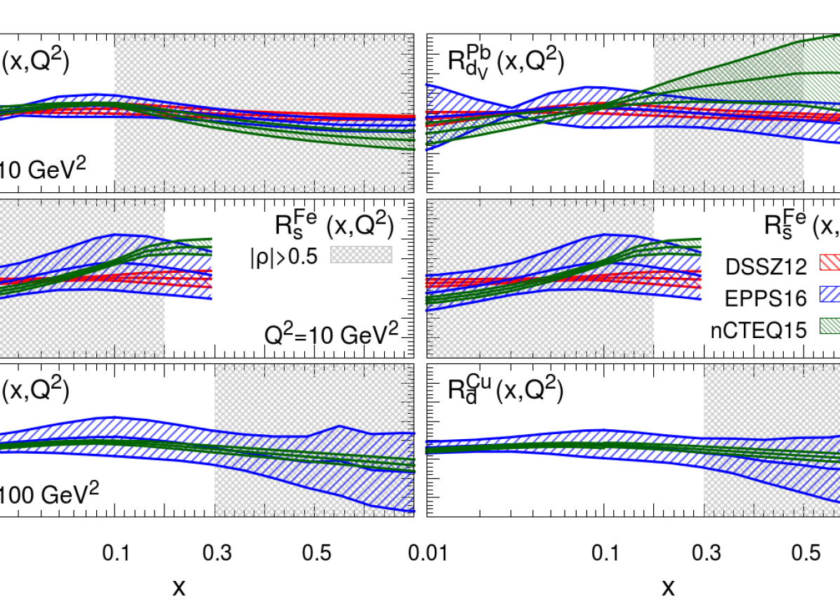
Figure 3: The ratio $R_{f}^{N}$ between the PDFs entering the nuclear and the proton observables, Eq. (9), for each of the nPDF sets considered in this analysis, and for the relevant flavours identified in Sect. 2.2. The shaded region corresponds to correlations $|\rho|>0.5$ between PDFs and observables, see also Fig. 2.

The observables entering Eqs. (6)-(8) are computed [58, 59] in exactly the same way for both proton and nuclear targets. Specifically, we always take into account the non-isoscalarity of the target, i.e., observables are averaged over proton and neutron contributions, weighted by the corresponding atomic and mass numbers $Z$ and $A$

$$T^{N}_{i}[f_{p}]=\frac{1}{A}\left\{ZT_{i}[f_{p}]+(A-Z)T_{i}[f_{n}]\right\}\,,\qquad T^{N}_{i}[f_{N}]=\frac{1}{A}\left\{ZT_{i}[f_{p/N}]+(A-Z)T_{i}[f_{n/N}]\right\}\,.$$ (10)

The nuclear PDF is simply

$$f_{N}=\frac{1}{A}\left[Zf_{p/N}+(A-Z)f_{n/N}\right]\,,$$ (11)

and thus the only difference between proton and nuclear observables consists of replacing the free-proton PDF, $f_{p}$, with the bound-proton PDF, $f_{p/N}$. In all these expressions free- and bound-neutron PDFs are computed from their proton counterparts by assuming exact isospin symmetry.

Initially, the free-proton PDF is taken from the NNPDF3.1 set, while the bound-proton PDF is obtained by applying to the same free-proton PDF the replica-by-replica nuclear correction $R_{f}^{N,(n)}(x,Q^{2})$ determined in Eq. (9):

$$f_{p/N}^{(n)}=R_{f}^{N,(n)}f_{p}\,.$$ (12)

In this procedure the input of the nuclear PDFs enters only through the correction Eq. (9). To ensure maximum theoretical consistency between proton and nuclear observables in Eqs. (6)-(8) and (10), they are each computed with the same theoretical settings as in the fit, see Sect. 3.1. The free-proton PDF $f_{p}$ used in Eqs. (10) and (12) is then iterated to consistency, i.e., the output of the free-proton fit (as described in Sect. 3 below) is used to compute the bound-proton PDF used in a subsequent fit. While in principle the PDF used in the determination of $R_{f}^{N,(n)}$ Eq. (9) should also be iterated, for consistency, in practice this is only a small correction since the dependence of $R_{f}^{N,(n)}$ on the input proton PDF is very weak.

2.3.3 Discussion

Before implementing the nuclear covariance matrix in a global fit of proton PDFs, we look more closely at the pattern of nuclear corrections, and at the nuisance parameters and shifts defined in Eqs. (6-8). In Fig. 3, we show the nuclear correction $R_{f}^{N}$, Eq (9). For each nuclear species, we display only the PDF flavours that are expected to give the largest contribution to the relevant observables, as outlined in Sect. 2.2. The ratio is computed, for each of the three nPDF sets selected in the previous section, at the typical average scale of the corresponding dataset: $Q^{2}=10$ GeV² for CHORUS and NuTeV, and $Q^{2}=100$ GeV² for E605. For each nPDF set, uncertainty bands correspond to the nominal tolerances discussed above, and and have been rescaled to $68\%$ CLs for nCTEQ15 and EPPS16. The most interesting region of maximal correlation between the PDFs and the observables (corresponding to $|\rho|>0.5$ in Fig. 2) is shown shaded. Since the observables depend linearly on the nuclear PDFs, the quantity defined in Eq. (9) provides an estimate of the relative size of the nuclear corrections. According to Fig. 3, we therefore expect moderate deviations for all the experiments.

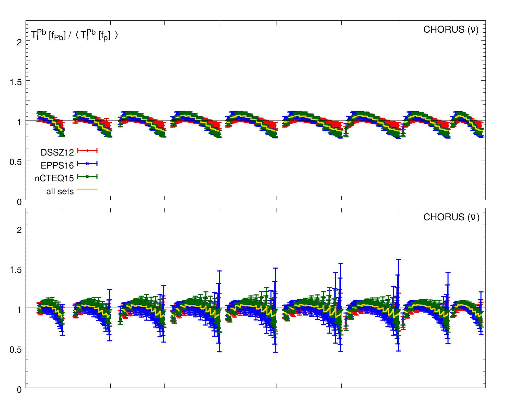
Figure 4: The ratio between the CHORUS observable computed with nuclear PDFs, $T_{i}^{\rm Pb}[f_{\rm Pb}]$, and the central prediction with proton PDFs, $\langle T_{i}^{\rm Pb}[f_{p}]\rangle$, in the case of neutrino (top) and antineutrino (bottom) beams. Results from the DSSZ12, EPPS16 and nCTEQ15 sets are displayed separately. The ratio between the nuclear and the proton expectation values is also shown, averaged over the combination of all replicas from all nPDF sets. In each plot there are nine bins corresponding to different energies of the neutrino/antineutrino beam $E_{\nu/\bar{\nu}}$: 25, 35, 45, 55,70, 90, 110, 130 and 170 GeV, respectively. In each bin, the $x$ value increases from left to right in the range displayed in Table 1, $0.045<x<0.65$. For clarity, the various bins are separated by a tick on the horizontal axis.

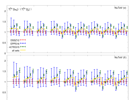
Figure 5: Same as Fig. 4, but for NuTeV. From left to right, there are nine bins corresponding to three different inelasticities $y$: 0.334, 0.573, 0.790, and three different neutrino/antineutrino beam energies $E_{\nu/\bar{\nu}}$: 90.18, 174.37 and 244.72 GeV. In each bin, the $x$ value increases from left to right in the range displayed in Table 1, $0.02<x<0.33$ for neutrinos, and $0.02<x<0.21$ for antineutrinos.

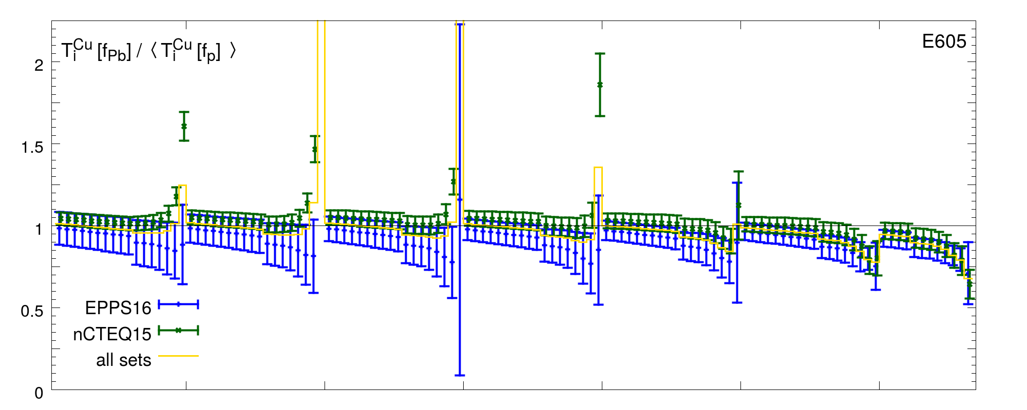
Figure 6: Same as Fig. 4, but for E605. From left to right, there are seven bins corresponding to different values of the vector boson rapidity $y$: -0.2, -0.1, 0.0, 0.1, 0.2, 0.3 and 0.4. In each bin, the value of the dilepton invariant mass $M_{\ell\ell}$ increases from left to right in the range displayed in Table 1, $7.1<M_{\ell\ell}<10.9$ GeV.

The nuclear corrections to the observables themselves are shown in Figs. 4-6, where, for each data point $i$ (after kinematic cuts) in the CHORUS, NuTeV and E605 datasets, we display the observables computed with nuclear PDFs, normalised to the expectation value with the proton PDF, $T_{i}^{N}[f_{N}]/\langle T_{i}^{N}[f_{p}]\rangle$. Results are shown for the DSSZ12, EPPS16 and nCTEQ15 sets separately. The central value of the same ratio obtained from the Monte Carlo combination of all the three nPDF sets is also shown. Looking at Figs. 4-6, we observe that the shape and size of the ratios between observables closely follow that of the ratios between PDFs in the shaded region of Fig. 3. For CHORUS, all the nPDFs modify the nuclear observable in a similar way, with a slight enhancement at smaller values of $x$, and a suppression at larger values of $x$. Overall, the uncertainty in the nuclear observable is comparable for the three sets. All sets are mutually consistent within uncertainties. For NuTeV, the nuclear corrections are markedly inconsistent for DSSZ12 and nCTEQ15, with the former being basically flat around one, while the latter deviates very significantly from one in some bins. Both nPDF sets are included within the much larger uncertainties of the EPPS16 set, which has now the largest stated uncertainty, especially in the case of antineutrino beams. This is likely a consequence of the fact that the strange quark nPDF was fitted independently from the other quark nPDFs in EPPS16, while it was related to lighter quark nPDFs in DSS12 and nCTEQ15 [26]. For E605, the nuclear correction gives a mild reduction in most of the measured kinematic range. The nCTEQ15 nPDF set appears to be more precise than the EPPS16 set, and they are reasonably consistent with each other. No DSSZ12 set is available for Cu. On average the size of the nuclear correction shift, as quantified by the ratio $T_{i}^{N}[f_{N}]/T_{i}^{N}[f_{p}]$, is of order $10\%$ for CHORUS, $20\%$ for NuTeV, and $5\%$ for E605.

To gain a further idea of the effects to be expected from the nuclear corrections, in Fig. 7 we show the square root of the diagonal elements of the experimental and theoretical covariance matrices, and their sum, each normalised to the central value of the experimental data: $\sqrt{{\rm cov}_{ii}}/D_{i}$ (where ${\rm cov}_{ii}$ is equivalent, respectively, to $C_{ii}$, $S_{ii}$ or $C_{ii}+S_{ii}$). The theoretical covariance matrix is computed with Eq. (5) using the nuisance parameters Eq. (6); the general pattern of the results does not change qualitatively if Eqs. (7)-(8) are used instead. The features observed in Figs. 4-6 are paralleled in Fig. (7); in particular, the dependence of the size of the nuclear uncertainties on the bin kinematics. Moreover we can now see that the nuclear uncertainties are much smaller than the data uncertainties for E605, while for CHORUS (particularly $\nu$) they can be comparable. However for NuTeV the nuclear uncertainties are rather larger than the experimental uncertainties. This suggests that the NuTeV data will have relatively less weight in the global fit once the nuclear uncertainties are accounted for.

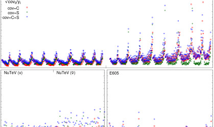
Figure 7: The square root of the diagonal elements of the covariance matrix normalised to the experimental data, $\sqrt{{\rm cov}_{ii}}/D_{i}$, for CHORUS, NuTeV and E605. We show results for the experimental covariance matrix, $C_{ij}$, for the nuclear covariance matrix, $S_{ij}$, computed from Eq. (6), and for their sum.

Finally, in Fig. 8 we show the experimental correlation matrices $\rho^{C}_{ij}=C_{ij}/\sqrt{C_{ii}C_{jj}}$ as heat plots: correlated points are red, while anti-correlated points are blue. For comparison we show the total correlation matrix obtained by summing the experimental and theoretical covariance matrices: $\rho^{C+S}_{ij}=(C_{ij}+S_{ij})/\sqrt{(C_{ii}+S_{ii})(C_{jj}+S_{jj})}$. These are computed according to Eq. (6) but the qualitative behaviour of the total correlation matrix is unaltered if Eqs. (7)-(8) are used instead. We see that our procedure captures the sizeable correlations of the nuclear corrections between different bins of momentum and energy, systematically enhancing bin-by-bin correlations in the data. Note as we might expect the nuclear uncertainties are strongly correlated between the different sets in the same experiment (i.e., neutrino and antineutrino sets in CHORUS and NuTeV). In principle, predictions for data points belonging to experiments that use different nuclear targets should be somewhat correlated, because part of the fit parameters in the nPDF analyses control the dependence on the nuclear mass number $A$. In order to be conservative, however, we do not attempt to include these correlations of the nuclear uncertainties between the experiments on different nuclear targets. If information were reliably included, it would reduce the overall effect of the nuclear uncertainty.

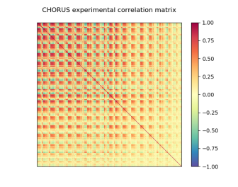
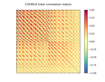
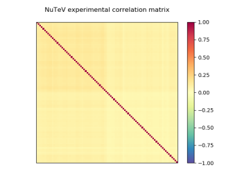
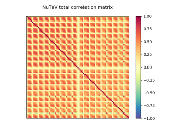
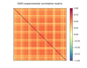
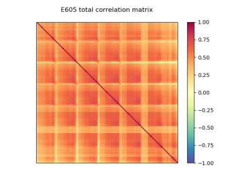
Figure 8: The experimental (left) and total (right) correlation matrices for CHORUS, NuTeV and E605. The theoretical covariance matrix, added to the experimental covariance matrix to obtain the total covariance matrix, is computed according to Eq. (6).

3 Impact of Theoretical Corrections in a Global PDF Fit

In this section, we discuss the impact of the theoretical uncertainties due to nuclear corrections, as computed in the previous section, in a global fit of proton PDFs. We first summarise the experimental and theoretical settings of the fits, then we present the results.

3.1 Fit Settings

The PDF sets discussed in this section are based on a variant of the NNLO NNPDF3.1 global analysis [3]. In particular the experimental input, and related kinematic cuts, are exactly the same as in the NNPDF3.1 NNLO fit. On top of the nuclear measurements presented in Sect. 2.2, the dataset is made up of: fixed-target [60, 27, 61, 62, 63, 15, 16, 17] and collider [64] DIS inclusive structure functions; charm and botton cross sections from HERA [65]; fixed-target DY cross sections [66, 67, 68]; gauge boson and inclusive jet production cross sections from the Tevatron [69, 70, 71, 72, 73]; and electroweak boson production, inclusive jet, $Z$ $p_{T}$, total and differential top-pair cross sections from ATLAS [74, 75, 76, 77, 78, 79, 80, 81, 82, 83, 84, 85, 86, 87, 88], CMS [89, 90, 91, 92, 93, 94, 95, 96, 97, 98, 99, 100] and LHCb [101, 102, 103, 104, 105]. The theoretical input is also the same as in NNPDF3.1: the strong running coupling at the $Z$-boson mass is fixed to $\alpha_{s}(m_{Z})=0.118$, consistent with the PDG average [106]; heavy-quark mass effects are included using the FONLL C general-mass scheme [107, 108], with pole masses $m_{c}=1.51$ GeV for charm and $m_{b}=4.92$ GeV for bottom, consistent with the Higgs cross section working group recommendation [109]; the charm PDF is fitted in the same way as the other light quark PDFs [110]; and the initial parametrisation scale is chosen just above the value of the charm mass, $Q_{0}=1.65$ GeV. All fits are performed at NNLO in pure QCD, and result in ensembles of $N_{\rm rep}=100$ replicas.

In comparison to NNPDF3.1, we have made small improvements in the computation of the CHORUS and NuTeV observables. In the case of CHORUS, cross sections were computed in NNPDF3.1 following the original implementation of Ref. [12], where the target was assumed to be isoscalar, and the data were supplemented with a systematic uncertainty to account for their actual non-isoscalarity. We now remove this uncertainty, and we compute the cross sections taking into account the non-isoscalarity of the target, as explained in Sect. 2.3.2. This increases the $\chi^{2}$ per data point a little (from $1.11$ to $1.25$). In the case of NuTeV, we update the value of the branching ratio of charmed hadrons into muons. This value, which is used to reconstruct charm production cross sections from the neutrino dimuon production cross sections measured by NuTeV, was set equal to $0.099$ in NNPDF3.1, following the original analysis of Ref. [8]. Previously, the uncertainty on the branching ratio was not taken into account. We now utilise the current PDG result, $0.086\pm 0.005$ [106], and include its uncertainty as an additional fully correlated systematic uncertainty. This reduces the $\chi^{2}$ per data point a little (from $0.82$ to $0.66$).

With these settings, we perform the following four fits:

• a Baseline fit, based on the theoretical and experimental inputs described above, and without any inclusion of theoretical nuclear uncertainties;

• a “No Nuclear” fit, NoNuc, equal to the Baseline, but without the datasets that utilise nuclear targets, i.e. without CHORUS, NuTeV and E605;

• a “Nuclear Uncertainties” fit, NucUnc, equal to the Baseline, but with the inclusion of theoretical nuclear uncertainties applied to CHORUS, NuTeV and E605, according to Eqs. (3)-(4), the theory covariance matrix being computed using (5) with the prescription Eq. (6) for the nuisance paremeters;

• a “Nuclear Corrections” fit, NucCor, equal to the Baseline, but with the inclusion of theoretical nuclear uncertainties applied to CHORUS, NuTeV and E605, according to Eqs. (3)-(4), with the nuclear correction $\delta T_{i}^{N}$, Eq. (8), added to the theoretical prediction $T_{i}[f]$ used in Eq. (4), and the theory covariance matrix computed using Eq. (5) and Eq. (7) for the nuisance parmeters.

The results of these fits are presented below.

3.2 Fit Quality and Parton Distributions

We first discuss the quality of the fits. In Table 3 we report the values of the $\chi^{2}$ per data point for each of the four fits listed above. Values are displayed for separate datasets, or groups of datasets corresponding to measurements of similar observables in the same experiment, and for the total dataset. We take into account all correlations in the computation of the experimental and/or theoretical covariance matrices entering the definition of the $\chi^{2}$, Eq. (4); multiplicative uncertainties are treated using the $t_{0}$ method [14], and two fit iterations are performed to ensure convergence of the final results.

Experiment	$N_{\rm dat}$	Baseline	NoNuc	NucUnc	NucCor
NMC	325	1.31	1.33	1.31	1.29
SLAC	67	0.79	0.93	0.72	0.73
BCDMS	581	1.23	1.17	1.20	1.21
CHORUS $\nu$	416	1.29	—	0.97	1.04
CHORUS $\bar{\nu}$	416	1.20	—	0.78	0.83
NuTeV dimuon $\nu$	39	0.41	—	0.31	0.40
NuTeV dimuon $\bar{\nu}$	37	0.90	—	0.62	0.83
HERA I+II incl.	1145	1.15	1.15	1.15	1.15
HERA $\sigma_{c}^{\rm NC}$	37	1.40	1.52	1.46	1.44
HERA $F_{2}^{b}$	29	1.11	1.10	1.10	1.11
E866 $\sigma^{d}_{\rm DY}/\sigma^{p}_{\rm DY}$	15	0.47	0.33	0.44	0.44
E886 $\sigma^{p}$	89	1.35	1.22	1.69	1.66
E605 $\sigma^{p}$	85	1.18	—	0.85	0.89
CDF $Z$ rap	29	1.41	1.29	1.39	1.41
CDF Run II $k_{t}$ jets	76	0.88	0.82	0.89	0.92
D0 $Z$ rap	28	0.60	0.57	0.59	0.59
D0 $W$ asy	17	2.11	2.06	2.10	2.09
ATLAS total	360	1.08	1.04	1.04	1.05
ATLAS $W,Z$ 7 TeV 2010	30	0.93	0.93	0.92	0.93
ATLAS HM DY 7 TeV	5	1.68	1.60	1.57	1.54
ATLAS low-mass DY 7 TeV	6	0.91	0.87	0.88	0.89
ATLAS $W,Z$ 7 TeV 2011	34	1.97	1.78	1.87	1.94
ATLAS jets	180	1.00	0.97	1.00	1.00
ATLAS $Z$ $p_{T}$ 8 TeV	92	0.93	0.95	0.95	0.92
ATLAS $t\bar{t}$	13	1.32	1.22	1.24	1.21
CMS total	409	1.07	1.07	1.07	1.07
CMS W asy	22	1.23	1.41	1.30	1.31
CMS Drell-Yan 2D 2011	110	1.30	1.33	1.31	1.29
CMS W rap 8 TeV	22	0.94	0.88	0.95	0.96
CMS jets	214	0.93	0.89	0.90	0.91
CMS $Z$ $p_{T}$ 8 TeV $(p_{T}^{ll},y_{ll})$	28	1.31	1.38	1.35	1.35
CMS $t\bar{t}$	13	0.77	0.73	0.76	0.75
LHCb total	85	1.46	1.27	1.32	1.37
LHCb $Z$	26	1.25	1.25	1.26	1.25
LHCb $W,Z\to\mu$	59	1.55	1.28	1.35	1.42
Total	4285	1.177	1.144	1.073	1.086

Table 3: The values of the $\chi^{2}$ per data point for the various fits described in the text. Data sets that utilise a nuclear target other than a deuteron are highlighted in boldface.

Inspection of Table 3 reveals that the global fit quality improves either if nuclear data are removed, or if they are retained with the supplemental theoretical uncertainty. The lowest global $\chi^{2}$ is obtained when the theoretical covariance matrix is included, with the deweighted implementation NucUnc leading to a slightly lower value than the corrected implementation NucCor. In all cases, the improvent is mostly driven by the fact that the $\chi^{2}$ for all the Tevatron and LHC hadron collider experiments decreases. This suggests that there might be some tension between nuclear and hadron collider data in the global fit.

Interestingly, however, the relatively poor $\chi^{2}$ of the ATLAS $W,Z$ 7 TeV 2011 dataset, which is sensitive to the strange PDF, only improves a little if the NuTeV dataset, which is also sensitive to the strange PDF, is either removed from the fit or supplemented with the theoretical uncertainty. This suggests that the poor $\chi^{2}$ of the ATLAS $W,Z$ 7 TeV 2011 dataset does not arise from tension with the NuTeV dataset. The two datasets are indeed sensitive to different kinematic regions, and there is little interplay between the two, as we will further demonstrate in Sect. 4.2.

The fit quality of the DIS and fixed-target DY data is stable across the fits. Fluctuations in the values of the corresponding $\chi^{2}$ are small, except for a slight worsening in the $\chi^{2}$ of the HERA charm cross sections and of the fixed-target proton DY cross section. Concerning nuclear datasets, their $\chi^{2}$ always decreases in the NucUnc and NucCor fits in comparison to the Baseline fit, with the size of the decrease being slightly larger in the NucUnc fit than in the NucCor fit. This suggests that when the shift is used as a nuclear correction, such a correction is reasonably reliable, in the sense that its uncertainty is not substantially underestimated. However, the NucUnc implementation is more conservative than the NucCor one, and leads to a better fit.

We now compare the PDFs obtained from the various fits, and study how their central values and uncertainties vary. To do so, we first inspect the distance between the Baseline and each of the other fits. The distance between two fits, defined, e.g., in Ref [111], quantifies their statistical equivalence. Specifically, for two PDF sets made of $N_{\rm rep}=100$ replicas, a distance of $d\simeq 1$ corresponds to statistically equivalent sets, while a distance of $d\simeq 10$ corresponds to sets that differ by one-sigma in units of the corresponding standard deviation. We display the distance between each pair of fits, both for the central value and for the uncertainty, in Fig. 9. Results are displayed as a function of $x$ at a representative scale of the nuclear dataset, $Q=10$ GeV, for all PDF flavours.

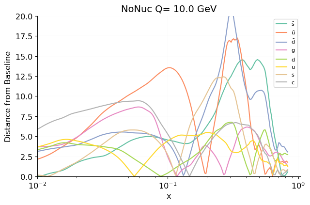
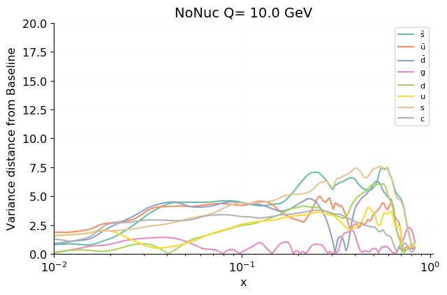
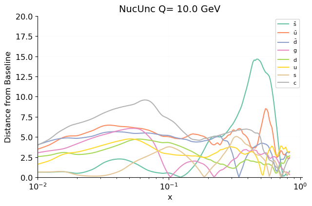
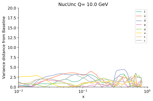
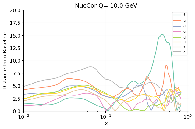
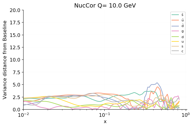
Figure 9: Distances between the central values (left) and the uncertainties (right) of the Baseline fit and the NoNuc (top), NucUnc (middle), and NucCor (bottom) fits, see text for details. Results are displayed as a function of $x$ at a representative scale of the nuclear dataset, $Q=10$ GeV, for all PDF flavours.

As expected, the largest distances with respect to the Baseline fit are displayed by sea quarks, at the level of both the central value and the uncertainty, to which the nuclear dataset is mostly sensitive. In the NoNuc fit, the central values of the $\bar{u}$, $\bar{d}$, $s$ and $\bar{s}$ quarks can differ by more than one sigma, while the distance in the corresponding uncertainties is more limited, albeit still around half a sigma, especially for $s$ and $\bar{s}$ PDFs. This confirms that nuclear data still have a sizeable weight in a global fit, as already noted in Sect. 4.11 of Ref. [3]. In the global fits including theoretical uncertainties from nuclear effects, the pattern of the distances to the Baseline is mostly insensitive to whether the nuclear effects are considered as an uncertainty or a correction. For the central value, distances are always below one sigma, except for the $\bar{s}$ PDF, where differences with respect to the Baseline fit exceed one sigma in the range $0.4\leq x\leq 0.6$. For the uncertainties, distances from the Baseline are comparable in the two fits NucUnc and NucCor, with $\bar{u}$, $\bar{d}$ $s$ and $\bar{s}$ PDFs displaying the largest values, which are however all no more than half a sigma.

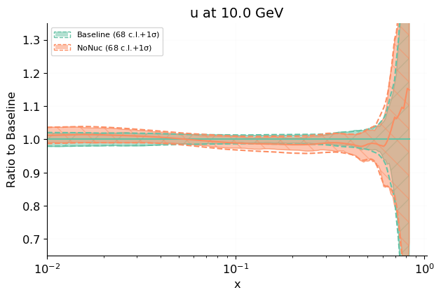
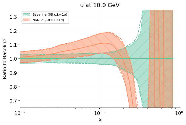
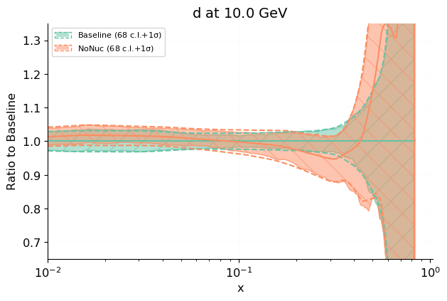
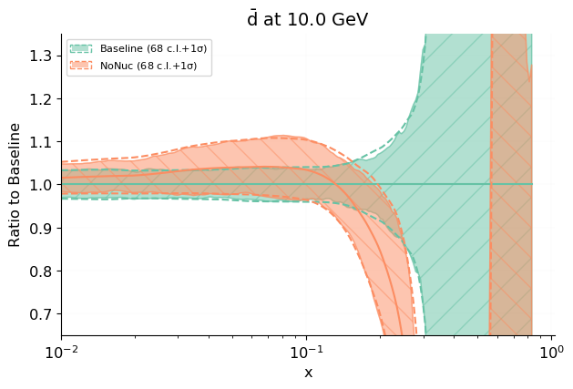
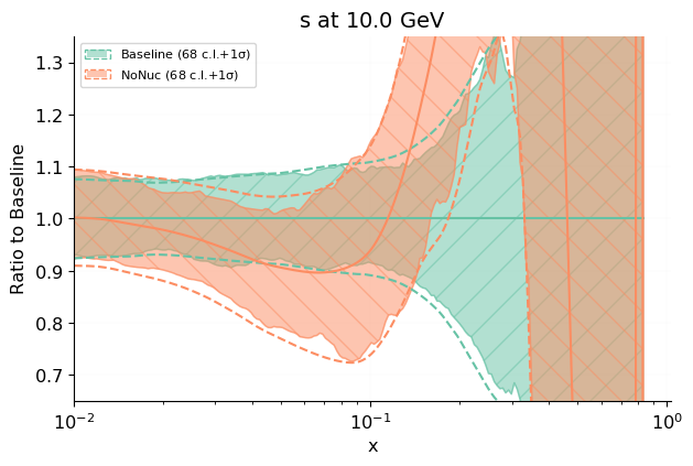
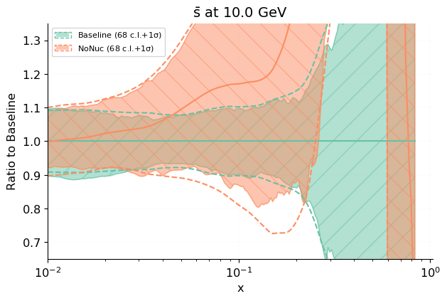
Figure 10: Comparison between the Baseline fit, and the fit without any data on nuclear targets, NoNuc. The light quark (left) and antiquark (right) flavours are shown at $Q=10$ GeV. Results are normalised to the Baseline fit.

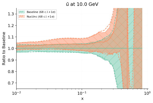
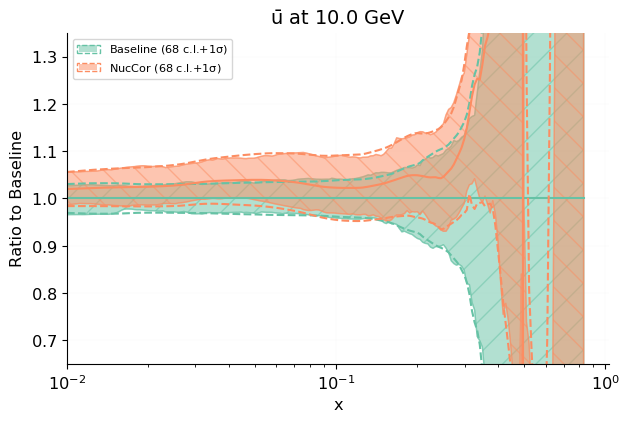
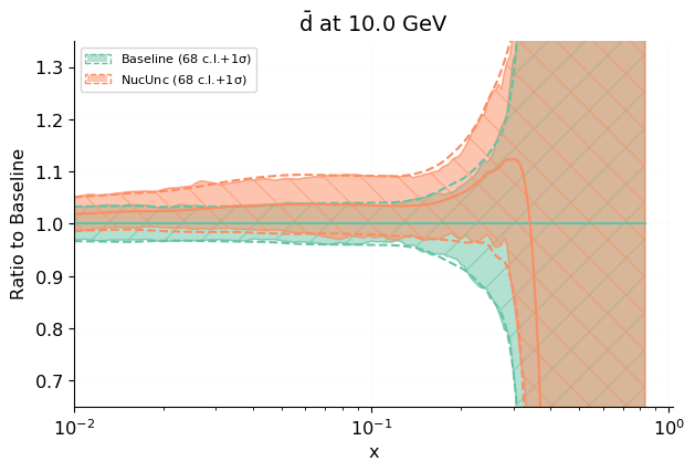
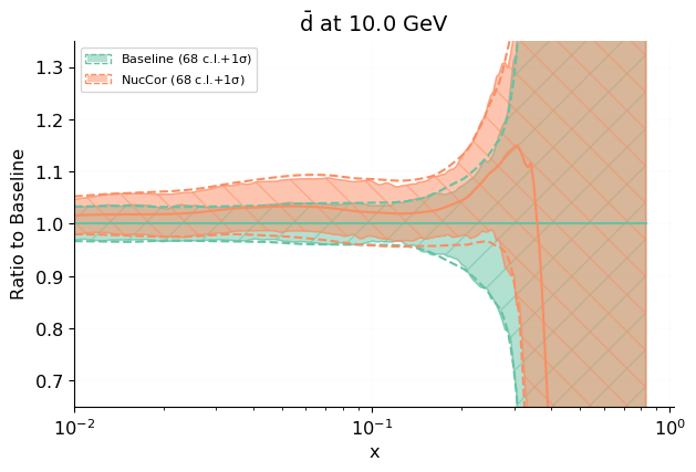
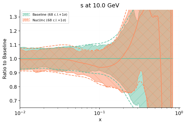
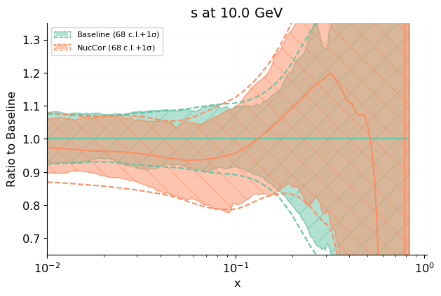
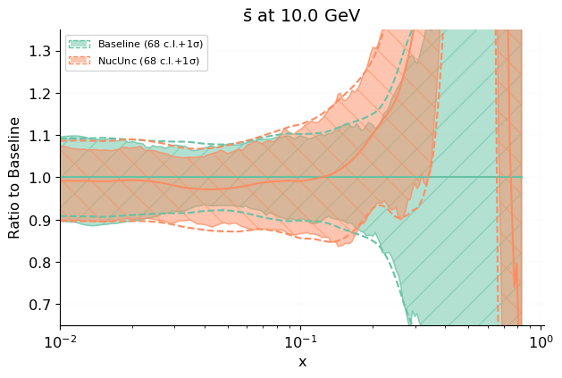
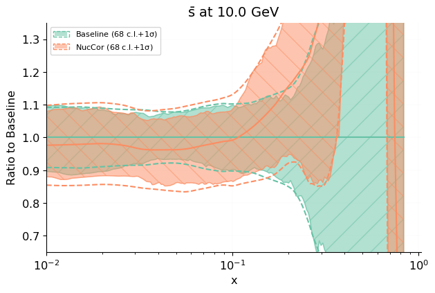
Figure 11: Comparison between the Baseline fit, and each fit including theoretical uncertainties, NucUnc (left), and NucCor (right). The antiup, antidown, strange and antistrange flavours are shown at $Q=10$ GeV from top to bottom. Results are normalised to the Baseline fit.

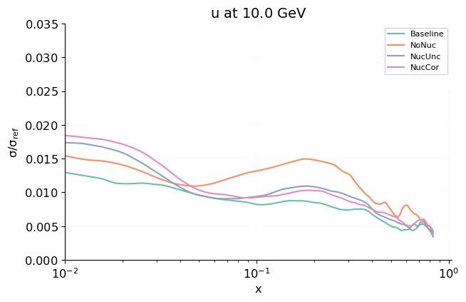
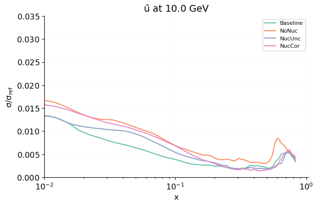
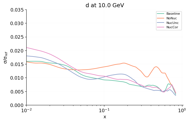
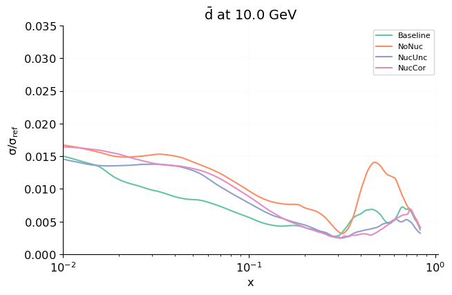
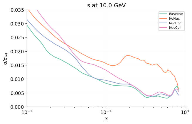
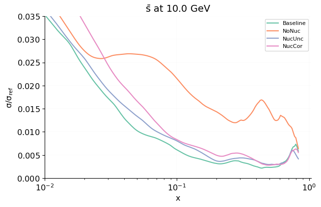
Figure 12: Comparison of the absolute PDF uncertainty for the light quark and antiquark flavours from the four fits performed in this analysis at $Q=10$ GeV.

We now make the most important differences in the PDF central values and uncertainties among the four fits explicit. In Fig. 10 we compare the light quark and antiquark PDFs between the Baseline and the NoNuc fits. In Fig. 11 we compare the sea quark PDFs between the Baseline and either the NucUnc or the NucCor fits. In both figures, results are normalised to the Baseline fit. In Fig. 12 we compare the absolute PDF uncertainty for the light quark and antiquark flavours from the four fits. All results are displayed at $Q=10$ GeV.

Inspecting Figs. 10-12 we may draw a number of conclusions. Firstly, the data taken on nuclear targets add a significant amount of information to the global fit. All light quark and antiquark PDFs are affected. The effect on the $u$ and $d$ PDFs, which are expected to be already very constrained by proton and deuteron data, consists of a slight distortion of the corresponding central values, which however remain always included in the one-sigma uncertainty of the comparing fit. More importantly, uncertainties are reduced by up to a factor of one third in the region $x\gtrsim 0.1$. The effect on the sea quark PDFs is more pronounced. Concerning central values, the nuclear data suppresses $\bar{u}$ and $\bar{d}$ PDFs below $x\sim 0.1$, and enhances them above $x\sim 0.1$. It also suppresses $s$ and $\bar{s}$ above $x\sim 0.1$. Uncertainties can be reduced down to two thirds (for $\bar{u}$ and $\bar{d}$) and to one quarter (for $s$ and $\bar{s}$) of the value obtained without the nuclear data. All these effects emphasise the constraining power of the nuclear data in a global fit, as already noted in Sect. 4.11 of Ref. [3].

Second, the inclusion of theoretical uncertainties in the fit mostly affects sea quark PDFs. Central values are generally contained within the one-sigma uncertainty of the Baseline fit, that includes the nuclear data but does not include any theoretical uncertainty, irrespective of the PDF flavour and of the prescription used to estimate the theoretical covariance matrix. The nature of the change in the central value is similar in both the NucUnc and the NucCor fits. For $\bar{u}$ and $\bar{d}$ PDFs, we observe an enhancement in the region $0.2\simeq x\simeq 0.3$ followed by a strong suppression for $x\gtrsim 0.3$. For $s$ and $\bar{s}$ PDFs, we observe: a slight suppression at $x\lesssim 0.1-0.2$; an enhancement at $0.1-0.2\lesssim x\lesssim 0.4-0.5$; and a strong suppression at $x\gtrsim 0.4-0.5$. Uncertainties are always increased when the theoretical covariance matrix is included in the fit, irrespective of the way it is estimated, for all PDF flavours. Such an increase is only marginally more apparent in the NucUnc fit, as a consequence of this being the more conservative estimate of the nuclear uncertainties.

All these effects lead us to conclude that theoretical uncertainties related to nuclear data are generally small in comparison to the experimental uncertainty of a typical global fit, in that deviations do not usually exceed one-sigma. Nevertheless, slight distortions in the central values and increases in the uncertainty bands (especially for $s$ and $\bar{s}$) become appreciable when theoretical uncertainties are taken into account. The systematic inclusion of nuclear uncertainties in a global fit is thus advantageous whenever conservative predictions of sea quark PDFs are required.

4 Impact on Phenomenology

As discussed in the previous section, the most sizeable impact of theoretical uncertainties is on the light sea quark PDFs, which display slightly distorted central values, and appreciably inflated uncertainties in comparison to the Baseline fit. In this section, we study the implications of these effects on the sea quark asymmetry, and on the strangeness fraction of the proton, including a possible asymmetry between $s$ and $\bar{s}$ PDFs.

4.1 The Sea Quark Asymmetry

A sizeable asymmetry in the antiup and antidown quark sea was observed long ago in DY first by the NA51 [112] and then by the NuSea/E866 experiments [113]. Perturbatively, the number of antiup and antidown quarks in the proton is expected to be very nearly the same, because they originate primarily from the splitting of gluons into a quark-antiquark pair, and because their masses are very small in comparison to the confinement scale. The observed asymmetry must therefore be explained by some non-perturbative mechanism, which has been formulated in terms of various models over the years [114].

While a complete understanding of this asymmetry is still lacking, we want to analyse here the effect of the nuclear data and of their associated theoretical uncertainties due to nuclear effects on the PDF determination of the ratio $\bar{d}/\bar{u}$. In Fig. 13 we show the ratio $\bar{d}/\bar{u}$ as a function of $x$ at two representative values of $Q$ for the nuclear data ($Q=10$ GeV), and for the collider data ($Q=91.2$ GeV). Results refer to the Baseline, NoNuc and NucUnc fits discussed in Sect. 3. We omit the NucCor result from Fig. 13 for readability, as it is almost indistinguishable from the NucUnc result.

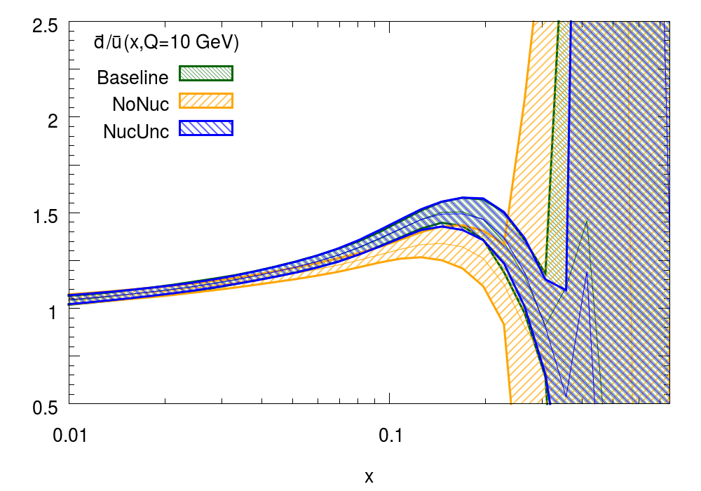
Figure 13: The ratio $\bar{d}/\bar{u}$ as a function of $x$ at two representative values of $Q$ for the nuclear data ($Q=10$ GeV) and for the collider data ($Q=91.2$ GeV).

Inspection of Fig. 13 makes it apparent that the effect of nuclear data on the $\bar{d}/\bar{u}$ ratio is significant, in particular in the region $0.03\lesssim x\lesssim 0.3$. In this region, the central value of the Baseline fit is enhanced by around two sigma with respect to the NoNuc fit. The corresponding uncertainty bands do not show any significant difference in size, but they barely overlap. The two fits differ by approximately $\sqrt{2}$ sigma. The inclusion of the nuclear uncertainty, even at its most conservative, makes little difference to the $\bar{d}/\bar{u}$ ratio: the central value and the uncertainty of the NucUnc result are almost unchanged in comparison to the Baseline, and the ratio remains significantly larger than the NoNuc result.

4.2 The Strange Content of the Proton Revisited

The size of the $s$ and $\bar{s}$ PDFs has recently been a source of some controversy. Specifically, for many years the fraction of strange quarks in the proton

$$R_{s}(x,Q^{2})=\frac{s(x,Q^{2})+\bar{s}(x,Q^{2})}{\bar{d}(x,Q^{2})+\bar{u}(x,Q^{2})}\,,$$ (13)

and the corresponding momentum fraction

$$K_{s}(Q^{2})=\frac{\int_{0}^{1}dx\ x\left[s(x,Q^{2})+\bar{s}(x,Q^{2})\right]}{\int_{0}^{1}dx\ x\left[\bar{u}(x,Q^{2})+\bar{d}(x,Q^{2})\right]}$$ (14)

have been found to be smaller than one in all global PDF sets in which strange PDFs are fitted. This result was mostly driven by NuTeV data, and has been understood to be due to the mass of the strange quark, which kinematically suppresses the production of $s$-$\bar{s}$ pairs. This orthodoxy was challenged in Ref. [115], where, on the basis of ATLAS $W$ and $Z$ production data combined with HERA DIS data, it was claimed that the strange fraction $R_{s}$ is of order one. The data of Ref. [115] was later included in the NNPDF3.0 global analysis [116], together with NuTeV data, to demonstrate that whereas the ATLAS data does favour a larger total strangeness, it has a moderate impact in the global fit due to its rather large uncertainties. Furthermore, in a variant of the NNPDF3.0 analysis, if the $s$ and $\bar{s}$ PDFs were determined from HERA and ATLAS data only, the central value of $R_{s}$ is consistent with the conclusion of Ref. [115], and its uncertainty is large enough to make it compatible with the result of the global fit. This state of affairs was reassessed in the NNDPF3.1 global analysis [3], where the ATLAS $W$ and $Z$ dataset was supplemented with the more precise measurements of Ref. [83]. They were found to enhance the total strangeness, consistently with that of Ref. [115], although their $\chi^{2}$ remained rather poor. This suggested some residual tension in the preferred total strangeness between the ATLAS data and the rest of the dataset, specifically NuTeV.

We might wonder whether, since the NuTeV data were taken on an iron target, the inclusion of nuclear uncertainties might reconcile this discrepancy. We therefore revisit the strange content of the proton, by computing the ratios $R_{s}$ and $K_{s}$, Eqs. (13)-(14), based on the four fits discused in the previous section at $Q=1.38$ GeV (below the charm threshold) and $Q=m_{Z}$, with $m_{Z}=91.2$ GeV the mass of the $Z$ boson. The values of $R_{s}$ at $x=0.023$ and of $K_{s}$ are collected in Table 4, where the determination of Ref. [83] is also shown. We display the ratio $R_{s}$ as a function of $x$ for the Baseline, NoNuc and NucUnc fits in Fig. 14. Again we omit the NucCor result from Fig. 14 for readability, as it is almost indistinguishable from the NucUnc result. The values of $Q$ and $x$ are the same as those used in the analysis of Ref. [83], where they were chosen to maximise sensitivity to either the nuclear (at low $Q$) or the collider (at high $Q$) data.

	Baseline	NoNuc	NucUnc	NucCor	Ref. [83]
$R_{s}(x=0.023,Q=1.38\text{ GeV})$	$+0.69\pm 0.15$	$+0.68\pm 0.14$	$+0.65\pm 0.14$	$+0.64\pm 0.15$	$+1.13\pm 0.11$
$R_{s}(x=0.023,Q=91.2\text{ GeV})$	$+0.81\pm 0.05$	$+0.79\pm 0.07$	$+0.79\pm 0.06$	$+0.77\pm 0.06$	—
$K_{s}(1.38\text{ GeV})$	$+0.63\pm 0.09$	$+0.97\pm 0.18$	$+0.63\pm 0.09$	$+0.61\pm 0.10$	—
$K_{s}(91.2\text{ GeV})$	$+0.80\pm 0.05$	$+0.98\pm 0.09$	$+0.80\pm 0.05$	$+0.79\pm 0.06$	—

Table 4: The fractions $R_{s}$, Eq. (13), and $K_{s}$, Eq. (14), for representative values of $x$ and $Q$.

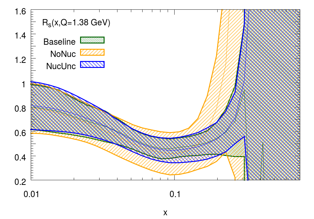
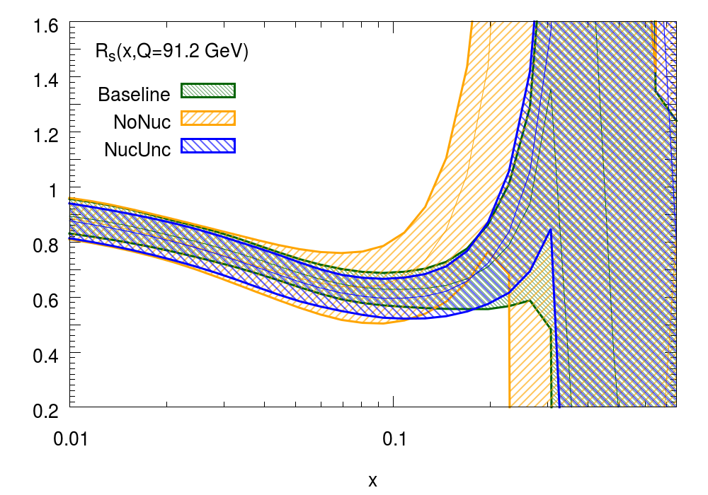
Figure 14: The fraction $R_{s}$, Eq. (13), as a function of $x$ at two representative values of $Q$ for the nuclear data ($Q=1.38$ GeV) and for the ATLAS $W$ $Z$ data ($Q=91.2$ GeV).

Inspection of Table 4 and Fig. 14 makes it apparent that the effect of nuclear data on $R_{s}$ at low values of $x$, namely at $x=0.023$, is negligible. The central values and the uncertainties of $R_{s}$ are remarkably stable across the four fits. This is unsurprising, as $x=0.023$ is at the lower edge of the kinematic region covered by the nuclear data, see Fig. 1. At larger values of $x$, instead, particularly in the range $0.03\lesssim x\lesssim 0.2$, the nuclear data affects $R_{s}$ quite significantly, as is apparent from comparison of the NoNuc and Baseline fits. In the Baseline (which includes the nuclear data), the uncertainty on $R_{s}$ is reduced by a factor of two without any apparent distortion of the central value. Likewise, the effect of nuclear uncertainties is mostly apparent in a similar $x$ range. If one compares the NucUnc and the Baseline fits, an increase of the uncertainty on $R_{s}$ by up to one third can be seen. However, this effect remains moderate, and is mostly washed out when it is integrated over the full range of $x$. The value of $K_{s}$ is indeed almost unchanged by the inclusion of nuclear uncertainties in the Baseline fit, irrespective of whether they are implemented as the NucUnc or the NucCor fit, especially at high values of $Q$.

We therefore conclude that the inclusion of nuclear uncertainties does nothing to reconcile the residual tension between ATLAS and NuTeV data, the reason being that they probe the strangeness in kinematic regions of $x$ and $Q$ that barely overlap. Further evidence of the limited interplay between ATLAS and NuTeV data is provided by the $\chi^{2}$ of the former, which remains poor for all the four fits considered in this analysis, see Table 3. Achieving a better description of the ATLAS data or an improved determination of the strange content of the proton might require the inclusion of QCD corrections beyond NNLO and/or of electroweak corrections, or the analysis of other processes sensitive to $s$ and $\bar{s}$ PDFs, such as kaon production in semi-inclusive DIS. All this remains beyond the scope of this work.

Finally, we investigate the effect of the nuclear data on the strange valence distribution $xs^{-}(x,Q)=x[s(x,Q)-\bar{s}(x,Q)]$, which we display as a function of $x$ at two representative values of $Q$ in Fig. 15. Results are shown for each of the four fits performed in this analysis. From Fig. 15, we see once again the constraining power of the nuclear data. By comparing the Baseline and the NoNuc fits, it is apparent that the strange valence distribution is almost unconstrained when the nuclear data is removed from the fit, with large uncertainty and completely unstable shape.

When the nuclear data is included, similar effects are observed whether nuclear uncertainties are implemented conservatively or as a correction. Concerning the central values, in comparison to the Baseline fit the NucUnc and NucCor fits have a slightly suppressed valence distribution in the region $x\lesssim 0.3$. Overall, nuclear effects do not alter the asymmetry between $s$ and $\bar{s}$ PDFs. Concerning the uncertainties themselves, both the NucUnc and the NucCor fits show an increased uncertainty in the strange valence distribution in the region $x\lesssim 0.3$, which is a little more pronounced for the the NucCor fit than the NucUnc fit, contrary to what would be expected if the small nuclear correction obtained from the nPDFs were a genuine effect.

In conclusion, nuclear effects have negligible impact on the $\bar{d}-\bar{u}$ asymmetry, on the total strangeness, and on the $s-\bar{s}$ asymmetry. We do not observe any evidence in support of the use of nuclear corrections (NucCor): in the global proton fit, the fit quality to the nuclear datasets (and the overall fit quality) is always a little worse when nuclear corrections are implemented. This may be due to the slight inconsistencies between the different sets of nPDFs, visible in Fig. 3. The use of the more conservative nuclear uncertainties (NucUnc) in global proton PDF fits is thus the recommended option, at least until more reliable nPDFs become available.

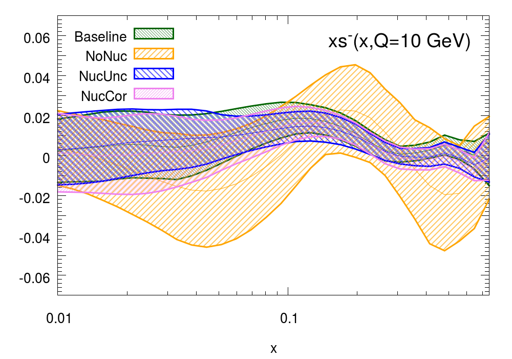
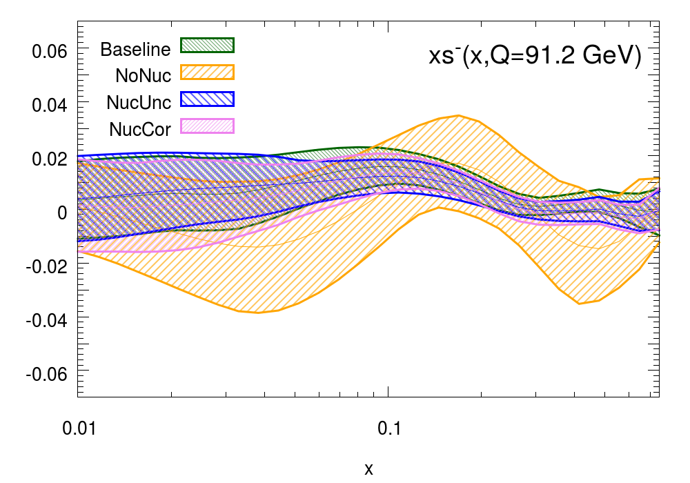
Figure 15: The strange valence distribution $xs^{-}(x,Q)=x[s(x,Q)-\bar{s}(x,Q)]$ as a function of $x$ at two values of $Q$: a typical scale for the nuclear data ($Q=10$ GeV), and for the collider data ($Q=91.2$ GeV).

5 Summary and Outlook

In this paper we revisited the rôle of the nuclear data commonly used in a global determination of proton PDFs. Specifically, we considered: DIS data taken with Pb and Fe targets, from CHORUS and NuTeV experiments, respectively; and DY data taken with a Cu target, from the E605 experiment. We studied the fit quality and the stability of the proton PDFs obtained in the framework of the NNDPF3.1 global analysis, by comparing a series of determinations: one in which the nuclear dataset is removed from the fit; one in which it is included without any nuclear correction (the baseline fit); and two in which it is included with a theoretical uncertainty that takes into account nuclear effects.

The two determinations which included a theoretical uncertainty were realised by constructing a theoretical covariance matrix that was added to the experimental covariance matrix, both when generating data replicas and when fitting PDFs. These covariance matrices were constructed using a Monte Carlo ensemble of nuclear PDFs, determined from a wide set of measurements using nuclear data. In the first determination, the theoretical covariance matrix elements were constructed by finding the difference between each nuclear PDF replica and a central proton PDF, and then taking an average over replicas. This gives a conservative estimate of the nuclear uncertainty, increasing uncertainties overall, and deweighting the nuclear data in the fit. In the second determination, the theoretical covariance matrix elements were constructed by finding the difference between each nuclear PDF replica and the central nuclear PDF. Additionally, the theoretical prediction was shifted by the difference between the predictions made with central nuclear and proton PDFs. This correction procedure takes the nuclear effects and their uncertainties as determined by the nuclear fits at face value, but is less conservative than the first prescription.

We confirm that the nuclear dataset contains substantial information on the proton PDFs, even when the uncertainties due to nuclear effects are taken into account. In particular it provides an important constraint on the light sea quark PDFs, consistent with constraints from LHC data, as we explicitly demonstrated by inspecting the individual PDFs, the $\bar{d}/\bar{u}$ ratio, the strangeness fractions $R_{s}$ and $K_{s}$, and the strange valence distribution $s-\bar{s}$. Therefore, it should not be dropped from current global PDF fits.

A conservative estimate of the additional theoretical uncertainty due to the use of a nuclear rather than a proton target in these measurements gives only small changes in the central values of the proton PDFs, with a slight increase in their overall uncertainties. In particular, nuclear effects are insufficient to explain any residual tension in the global fit between fixed target and ATLAS determinations of the strangeness content of the proton. This is largely because the corresponding measurements are sensitive to different kinematic regions that have a limited interplay. We nevertheless recommend that nuclear uncertainties are always included in future global fits, to eliminate any slight bias, and as a precaution against underestimation of uncertainties.

We should emphasise that all our results were determined from the most recent publically available nuclear PDFs. Despite the fact that these are obtained from a global analysis of experimental data taken in a wide variety of processes, including DIS, DY and $pN$ collisions, some inconsistencies between the nPDF sets, in particular in the estimation of the uncertainties, were observed. This suggests that nPDFs are not yet sufficiently reliable to justify the use of a nuclear correction in the fit. Indeed, when we attempted to use them to give a nuclear correction to the predictions with proton PDFs, the fit quality was always a little worse than that obtained without nuclear corrections. Even so, the effect on the proton PDFs, in particular the $\bar{d}/\bar{u}$ ratio, the total strangeness $s+\bar{s}$, and the valence strange distribution $s-\bar{s}$ was negligible. Nevertheless, we recommend that when estimating nuclear effects using current nPDF sets, the more conservative approach is adopted, in which nuclear effects give an additional uncertainty, but not a correction.

Our work can be extended in various different directions. First, we intend to reconsider our results when newer more reliable nPDF sets become available. In this respect, a consistent determination based on the NNPDF methodology [117] would be particularly helpful, both because it would give a more reliable assessment of the uncertainties on nPDFs, and because a consistent treatment, determining proton PDFs, nPDFs and nuclear corrections iteratively, would then be possible.

Second, our analysis can be extended to deuterium data. In principle, this suffers from similar uncertainties as the nuclear data considered here, though they are expected to be much smaller. Theoretical uncertainties might be estimated by studying the spread between various model predictions for nuclear effects, or by attempting to determine them empirically from the data, in iterating them to consistency with the proton data.

Finally, the general method of accounting for theoretical uncertainties in a PDF fit by estimating a theoretical covariance matrix that is added to the experimental one in the definition of the $\chi^{2}$ can have many other applications [11]: missing higher-order uncertainties [118], higher-twist uncertainties, and fragmentation function uncertainties in the analysis of semi-inclusive data. In this last respect, the analysis of kaon production data might be useful to obtain more information on the strangeness content of the proton.

The PDF sets presented in this work are available in the LHAPDF format [119] from the authors upon request.

References

- [1] J. Butterworth et al., PDF4LHC recommendations for LHC Run II, J. Phys. G43 (2016) 023001, [arXiv:1510.03865].
- [2] J. Gao, L. Harland-Lang, and J. Rojo, The Structure of the Proton in the LHC Precision Era, arXiv:1709.04922.
- [3] NNPDF Collaboration, R. D. Ball et al., Parton distributions from high-precision collider data, Eur. Phys. J. C77 (2017), no. 10 663, [arXiv:1706.00428].
- [4] L. A. Harland-Lang, A. D. Martin, P. Motylinski, and R. S. Thorne, Parton distributions in the LHC era: MMHT 2014 PDFs, Eur. Phys. J. C75 (2015), no. 5 204, [arXiv:1412.3989].
- [5] S. Dulat, T.-J. Hou, J. Gao, M. Guzzi, J. Huston, P. Nadolsky, J. Pumplin, C. Schmidt, D. Stump, and C. P. Yuan, New parton distribution functions from a global analysis of quantum chromodynamics, Phys. Rev. D93 (2016), no. 3 033006, [arXiv:1506.07443].
- [6] S. Alekhin, J. Blümlein, S. Moch, and R. Placakyte, Parton distribution functions, , and heavy-quark masses for LHC Run II, Phys. Rev. D96 (2017), no. 1 014011, [arXiv:1701.05838].
- [7] A. Accardi, L. T. Brady, W. Melnitchouk, J. F. Owens, and N. Sato, Constraints on large- parton distributions from new weak boson production and deep-inelastic scattering data, Phys. Rev. D93 (2016), no. 11 114017, [arXiv:1602.03154].
- [8] NNPDF Collaboration, R. D. Ball, L. Del Debbio, S. Forte, A. Guffanti, J. I. Latorre, A. Piccione, J. Rojo, and M. Ubiali, Precision determination of electroweak parameters and the strange content of the proton from neutrino deep-inelastic scattering, Nucl. Phys. B823 (2009) 195–233, [arXiv:0906.1958].
- [9] NNPDF Collaboration, R. D. Ball, V. Bertone, L. Del Debbio, S. Forte, A. Guffanti, J. Rojo, and M. Ubiali, Theoretical issues in PDF determination and associated uncertainties, Phys. Lett. B723 (2013) 330–339, [arXiv:1303.1189].
- [10] J. F. Owens, A. Accardi, and W. Melnitchouk, Global parton distributions with nuclear and finite- corrections, Phys. Rev. D87 (2013), no. 9 094012, [arXiv:1212.1702].
- [11] R. D. Ball and A. Deshpande, The Proton Spin, Semi-Inclusive processes, and a future Electron Ion Collider, 2018. arXiv:1801.04842.
- [12] NNPDF Collaboration, R. D. Ball, L. Del Debbio, S. Forte, A. Guffanti, J. I. Latorre, A. Piccione, J. Rojo, and M. Ubiali, A Determination of parton distributions with faithful uncertainty estimation, Nucl. Phys. B809 (2009) 1–63, [arXiv:0808.1231]. [Erratum: Nucl. Phys.B816,293(2009)].
- [13] G. D’Agostini, Bayesian reasoning in data analysis: A critical introduction. 2003.
- [14] NNPDF Collaboration, R. D. Ball, L. Del Debbio, S. Forte, A. Guffanti, J. I. Latorre, J. Rojo, and M. Ubiali, Fitting Parton Distribution Data with Multiplicative Normalization Uncertainties, JHEP 05 (2010) 075, [arXiv:0912.2276].
- [15] CHORUS Collaboration, G. Onengut et al., Measurement of nucleon structure functions in neutrino scattering, Phys. Lett. B632 (2006) 65–75.
- [16] NuTeV Collaboration, M. Goncharov et al., Precise measurement of dimuon production cross-sections in muon neutrino Fe and muon anti-neutrino Fe deep inelastic scattering at the Tevatron, Phys. Rev. D64 (2001) 112006, [hep-ex/0102049].
- [17] D. A. Mason, Measurement of the strange - antistrange asymmetry at NLO in QCD from NuTeV dimuon data. PhD thesis, Oregon U., 2006.
- [18] G. Moreno et al., Dimuon production in proton - copper collisions at = 38.8-GeV, Phys. Rev. D43 (1991) 2815–2836.
- [19] J. P. Berge et al., A Measurement of Differential Cross-Sections and Nucleon Structure Functions in Charged Current Neutrino Interactions on Iron, Z. Phys. C49 (1991) 187–224.
- [20] A. Guffanti and J. Rojo, Top production at the LHC: The Impact of PDF uncertainties and correlations, Nuovo Cim. C033 (2010), no. 4 65–72, [arXiv:1008.4671].
- [21] M. Arneodo, Nuclear effects in structure functions, Phys. Rept. 240 (1994) 301–393.
- [22] D. de Florian, R. Sassot, P. Zurita, and M. Stratmann, Global Analysis of Nuclear Parton Distributions, Phys. Rev. D85 (2012) 074028, [arXiv:1112.6324].
- [23] K. Kovarik et al., nCTEQ15 - Global analysis of nuclear parton distributions with uncertainties in the CTEQ framework, Phys. Rev. D93 (2016), no. 8 085037, [arXiv:1509.00792].
- [24] K. J. Eskola, P. Paakkinen, H. Paukkunen, and C. A. Salgado, EPPS16: Nuclear parton distributions with LHC data, Eur. Phys. J. C77 (2017), no. 3 163, [arXiv:1612.05741].
- [25] H. Paukkunen, Status of nuclear PDFs after the first LHC p–Pb run, Nucl. Phys. A967 (2017) 241–248, [arXiv:1704.04036].
- [26] H. Paukkunen, Nuclear PDFs Today, in 9th International Conference on Hard and Electromagnetic Probes of High-Energy Nuclear Collisions: Hard Probes 2018 (HP2018) Aix-Les-Bains, Savoie, France, October 1-5, 2018, 2018. arXiv:1811.01976.
- [27] New Muon Collaboration, M. Arneodo et al., Measurement of the proton and deuteron structure functions, F2(p) and F2(d), and of the ratio sigma-L / sigma-T, Nucl. Phys. B483 (1997) 3–43, [hep-ph/9610231].
- [28] New Muon Collaboration, P. Amaudruz et al., A Reevaluation of the nuclear structure function ratios for D, He, Li-6, C and Ca, Nucl. Phys. B441 (1995) 3–11, [hep-ph/9503291].
- [29] J. Gomez et al., Measurement of the A-dependence of deep inelastic electron scattering, Phys. Rev. D49 (1994) 4348–4372.
- [30] HERMES Collaboration, A. Airapetian et al., Measurement of R = sigma(L) / sigma(T) in deep inelastic scattering on nuclei, hep-ex/0210068.
- [31] New Muon Collaboration, M. Arneodo et al., The Structure Function ratios F2(li) / F2(D) and F2(C) / F2(D) at small x, Nucl. Phys. B441 (1995) 12–30, [hep-ex/9504002].
- [32] E665 Collaboration, M. R. Adams et al., Shadowing in inelastic scattering of muons on carbon, calcium and lead at low x(Bj), Z. Phys. C67 (1995) 403–410, [hep-ex/9505006].
- [33] European Muon Collaboration, J. Ashman et al., Measurement of the Ratios of Deep Inelastic Muon-Nucleus Cross-Sections on Various Nuclei Compared to Deuterium, Phys. Lett. B202 (1988) 603–610.
- [34] BCDMS Collaboration, G. Bari et al., A Measurement of Nuclear Effects in Deep Inelastic Muon Scattering on Deuterium, Nitrogen and Iron Targets, Phys. Lett. 163B (1985) 282.
- [35] A. Bodek et al., Electron Scattering from Nuclear Targets and Quark Distributions in Nuclei, Phys. Rev. Lett. 50 (1983) 1431.
- [36] BCDMS Collaboration, A. C. Benvenuti et al., Nuclear Effects in Deep Inelastic Muon Scattering on Deuterium and Iron Targets, Phys. Lett. B189 (1987) 483–487.
- [37] European Muon Collaboration, J. Ashman et al., A Measurement of the ratio of the nucleon structure function in copper and deuterium, Z. Phys. C57 (1993) 211–218.
- [38] New Muon Collaboration, M. Arneodo et al., The A dependence of the nuclear structure function ratios, Nucl. Phys. B481 (1996) 3–22.
- [39] New Muon Collaboration, M. Arneodo et al., The Q**2 dependence of the structure function ratio F2 Sn / F2 C and the difference R Sn - R C in deep inelastic muon scattering, Nucl. Phys. B481 (1996) 23–39.
- [40] NuTeV Collaboration, M. Tzanov et al., Precise measurement of neutrino and anti-neutrino differential cross sections, Phys. Rev. D74 (2006) 012008, [hep-ex/0509010].
- [41] D. M. Alde et al., Nuclear dependence of dimuon production at 800-GeV. FNAL-772 experiment, Phys. Rev. Lett. 64 (1990) 2479–2482.
- [42] NuSea Collaboration, M. A. Vasilev et al., Parton energy loss limits and shadowing in Drell-Yan dimuon production, Phys. Rev. Lett. 83 (1999) 2304–2307, [hep-ex/9906010].
- [43] PHENIX Collaboration, S. S. Adler et al., Centrality dependence of pi0 and eta production at large transverse momentum in s(NN)**(1/2) = 200-GeV d+Au collisions, Phys. Rev. Lett. 98 (2007) 172302, [nucl-ex/0610036].
- [44] STAR Collaboration, B. I. Abelev et al., Inclusive , , and direct photon production at high transverse momentum in and Au collisions at GeV, Phys. Rev. C81 (2010) 064904, [arXiv:0912.3838].
- [45] NA10 Collaboration, P. Bordalo et al., Nuclear Effects on the Nucleon Structure Functions in Hadronic High Mass Dimuon Production, Phys. Lett. B193 (1987) 368.
- [46] J. G. Heinrich et al., Measurement of the Ratio of Sea to Valence Quarks in the Nucleon, Phys. Rev. Lett. 63 (1989) 356–359.
- [47] NA3 Collaboration, J. Badier et al., Test of Nuclear Effects in Hadronic Dimuon Production, Phys. Lett. 104B (1981) 335. [,807(1981)].
- [48] CMS Collaboration, V. Khachatryan et al., Study of W boson production in pPb collisions at 5.02 TeV, Phys. Lett. B750 (2015) 565–586, [arXiv:1503.05825].
- [49] CMS Collaboration, V. Khachatryan et al., Study of Z boson production in pPb collisions at TeV, Phys. Lett. B759 (2016) 36–57, [arXiv:1512.06461].
- [50] ATLAS Collaboration, G. Aad et al., boson production in Pb collisions at TeV measured with the ATLAS detector, Phys. Rev. C92 (2015), no. 4 044915, [arXiv:1507.06232].
- [51] R. Sassot, M. Stratmann, and P. Zurita, Fragmentations Functions in Nuclear Media, Phys. Rev. D81 (2010) 054001, [arXiv:0912.1311].
- [52] R. Sassot. Private communication.
- [53] G. Watt and R. S. Thorne, Study of Monte Carlo approach to experimental uncertainty propagation with MSTW 2008 PDFs, JHEP 08 (2012) 052, [arXiv:1205.4024].
- [54] T.-J. Hou et al., Reconstruction of Monte Carlo replicas from Hessian parton distributions, JHEP 03 (2017) 099, [arXiv:1607.06066].
- [55] S. Carrazza, J. I. Latorre, J. Rojo, and G. Watt, A compression algorithm for the combination of PDF sets, Eur. Phys. J. C75 (2015) 474, [arXiv:1504.06469].
- [56] J. F. Owens, J. Huston, C. E. Keppel, S. Kuhlmann, J. G. Morfin, F. Olness, J. Pumplin, and D. Stump, The Impact of new neutrino DIS and Drell-Yan data on large-x parton distributions, Phys. Rev. D75 (2007) 054030, [hep-ph/0702159].
- [57] A. D. Martin, W. J. Stirling, R. S. Thorne, and G. Watt, Parton distributions for the LHC, Eur. Phys. J. C63 (2009) 189–285, [arXiv:0901.0002].
- [58] V. Bertone, S. Carrazza, and J. Rojo, APFEL: A PDF Evolution Library with QED corrections, Comput. Phys. Commun. 185 (2014) 1647–1668, [arXiv:1310.1394].
- [59] Z. Kassabov, Reportengine: A framework for declarative data analysis, Feb., 2019.
- [60] New Muon Collaboration, M. Arneodo et al., Accurate measurement of F2(d) / F2(p) and R**d - R**p, Nucl. Phys. B487 (1997) 3–26, [hep-ex/9611022].
- [61] BCDMS Collaboration, A. C. Benvenuti et al., A High Statistics Measurement of the Proton Structure Functions F(2) (x, Q**2) and R from Deep Inelastic Muon Scattering at High Q**2, Phys. Lett. B223 (1989) 485–489.
- [62] BCDMS Collaboration, A. C. Benvenuti et al., A High Statistics Measurement of the Deuteron Structure Functions F2 (X, ) and R From Deep Inelastic Muon Scattering at High , Phys. Lett. B237 (1990) 592–598.
- [63] L. W. Whitlow, E. M. Riordan, S. Dasu, S. Rock, and A. Bodek, Precise measurements of the proton and deuteron structure functions from a global analysis of the SLAC deep inelastic electron scattering cross-sections, Phys. Lett. B282 (1992) 475–482.
- [64] ZEUS, H1 Collaboration, H. Abramowicz et al., Combination of measurements of inclusive deep inelastic scattering cross sections and QCD analysis of HERA data, Eur. Phys. J. C75 (2015), no. 12 580, [arXiv:1506.06042].
- [65] ZEUS, H1 Collaboration, H. Abramowicz et al., Combination and QCD Analysis of Charm Production Cross Section Measurements in Deep-Inelastic ep Scattering at HERA, Eur. Phys. J. C73 (2013), no. 2 2311, [arXiv:1211.1182].
- [66] NuSea Collaboration, J. C. Webb et al., Absolute Drell-Yan dimuon cross-sections in 800 GeV / c pp and pd collisions, hep-ex/0302019.
- [67] J. C. Webb, Measurement of continuum dimuon production in 800-GeV/C proton nucleon collisions. PhD thesis, New Mexico State U., 2003. hep-ex/0301031.
- [68] NuSea Collaboration, R. S. Towell et al., Improved measurement of the anti-d / anti-u asymmetry in the nucleon sea, Phys. Rev. D64 (2001) 052002, [hep-ex/0103030].
- [69] CDF Collaboration, T. A. Aaltonen et al., Measurement of of Drell-Yan pairs in the Mass Region from Collisions at TeV, Phys. Lett. B692 (2010) 232–239, [arXiv:0908.3914].
- [70] D0 Collaboration, V. M. Abazov et al., Measurement of the shape of the boson rapidity distribution for + events produced at of 1.96 TeV, Phys. Rev. D76 (2007) 012003, [hep-ex/0702025].
- [71] CDF Collaboration, T. Aaltonen et al., Measurement of the Inclusive Jet Cross Section at the Fermilab Tevatron p anti-p Collider Using a Cone-Based Jet Algorithm, Phys. Rev. D78 (2008) 052006, [arXiv:0807.2204]. [Erratum: Phys. Rev.D79,119902(2009)].
- [72] D0 Collaboration, V. M. Abazov et al., Measurement of the muon charge asymmetry in W+X + X events at =1.96 TeV, Phys. Rev. D88 (2013) 091102, [arXiv:1309.2591].
- [73] D0 Collaboration, V. M. Abazov et al., Measurement of the electron charge asymmetry in decays in collisions at TeV, Phys. Rev. D91 (2015), no. 3 032007, [arXiv:1412.2862]. [Erratum: Phys. Rev.D91,no.7,079901(2015)].
- [74] ATLAS Collaboration, G. Aad et al., Measurement of the inclusive and Z/gamma cross sections in the electron and muon decay channels in collisions at TeV with the ATLAS detector, Phys. Rev. D85 (2012) 072004, [arXiv:1109.5141].
- [75] ATLAS Collaboration, G. Aad et al., Measurement of the high-mass Drell–Yan differential cross-section in pp collisions at =7 TeV with the ATLAS detector, Phys. Lett. B725 (2013) 223–242, [arXiv:1305.4192].
- [76] ATLAS Collaboration, G. Aad et al., Measurement of the Transverse Momentum Distribution of Bosons in Collisions at TeV with the ATLAS Detector, Phys. Rev. D85 (2012) 012005, [arXiv:1108.6308].
- [77] ATLAS Collaboration, G. Aad et al., Measurement of inclusive jet and dijet production in collisions at TeV using the ATLAS detector, Phys. Rev. D86 (2012) 014022, [arXiv:1112.6297].
- [78] ATLAS Collaboration, G. Aad et al., Measurement of the inclusive jet cross section in pp collisions at =2.76 TeV and comparison to the inclusive jet cross section at =7 TeV using the ATLAS detector, Eur. Phys. J. C73 (2013), no. 8 2509, [arXiv:1304.4739].
- [79] ATLAS Collaboration, G. Aad et al., Measurement of the cross section for top-quark pair production in collisions at TeV with the ATLAS detector using final states with two high-pt leptons, JHEP 05 (2012) 059, [arXiv:1202.4892].
- [80] ATLAS Collaboration, Measurement of the ttbar production cross-section in pp collisions at = 7 TeV using kinematic information of lepton+jets events, .
- [81] ATLAS Collaboration, T. A. collaboration, Measurement of the production cross-section in collisions at TeV using events with -tagged jets, .
- [82] ATLAS Collaboration, G. Aad et al., Measurement of the transverse momentum and distributions of Drell–Yan lepton pairs in proton–proton collisions at TeV with the ATLAS detector, Eur. Phys. J. C76 (2016), no. 5 291, [arXiv:1512.02192].
- [83] ATLAS Collaboration, M. Aaboud et al., Precision measurement and interpretation of inclusive , and production cross sections with the ATLAS detector, Eur. Phys. J. C77 (2017), no. 6 367, [arXiv:1612.03016].
- [84] ATLAS Collaboration, G. Aad et al., Measurement of the production cross-section using events with b-tagged jets in pp collisions at = 7 and 8 with the ATLAS detector, Eur. Phys. J. C74 (2014), no. 10 3109, [arXiv:1406.5375]. [Addendum: Eur. Phys. J.C76,no.11,642(2016)].
- [85] ATLAS Collaboration, M. Aaboud et al., Measurement of the production cross-section using events with b-tagged jets in pp collisions at =13 TeV with the ATLAS detector, Phys. Lett. B761 (2016) 136–157, [arXiv:1606.02699]. [Erratum: Phys. Lett.B772,879(2017)].
- [86] ATLAS Collaboration, G. Aad et al., Measurements of top-quark pair differential cross-sections in the lepton+jets channel in collisions at TeV using the ATLAS detector, Eur. Phys. J. C76 (2016), no. 10 538, [arXiv:1511.04716].
- [87] ATLAS Collaboration, G. Aad et al., Measurement of the low-mass Drell-Yan differential cross section at = 7 TeV using the ATLAS detector, JHEP 06 (2014) 112, [arXiv:1404.1212].
- [88] ATLAS Collaboration, G. Aad et al., Measurement of the boson transverse momentum distribution in collisions at = 7 TeV with the ATLAS detector, JHEP 09 (2014) 145, [arXiv:1406.3660].
- [89] CMS Collaboration, S. Chatrchyan et al., Measurement of the electron charge asymmetry in inclusive production in collisions at TeV, Phys. Rev. Lett. 109 (2012) 111806, [arXiv:1206.2598].
- [90] CMS Collaboration, S. Chatrchyan et al., Measurement of the muon charge asymmetry in inclusive production at 7 TeV and an improved determination of light parton distribution functions, Phys. Rev. D90 (2014), no. 3 032004, [arXiv:1312.6283].
- [91] CMS Collaboration, S. Chatrchyan et al., Measurement of the differential and double-differential Drell-Yan cross sections in proton-proton collisions at 7 TeV, JHEP 12 (2013) 030, [arXiv:1310.7291].
- [92] CMS Collaboration, S. Chatrchyan et al., Measurement of associated W + charm production in pp collisions at = 7 TeV, JHEP 02 (2014) 013, [arXiv:1310.1138].
- [93] CMS Collaboration, S. Chatrchyan et al., Measurement of the production cross section in the dilepton channel in pp collisions at = 8 TeV, JHEP 02 (2014) 024, [arXiv:1312.7582]. [Erratum: JHEP02,102(2014)].
- [94] CMS Collaboration, S. Chatrchyan et al., Measurement of the production cross section in the dilepton channel in collisions at TeV, JHEP 11 (2012) 067, [arXiv:1208.2671].
- [95] CMS Collaboration, S. Chatrchyan et al., Measurement of the production cross section in collisions at TeV with lepton + jets final states, Phys. Lett. B720 (2013) 83–104, [arXiv:1212.6682].
- [96] CMS Collaboration, V. Khachatryan et al., Measurement of the differential cross section and charge asymmetry for inclusive production at TeV, Eur. Phys. J. C76 (2016), no. 8 469, [arXiv:1603.01803].
- [97] CMS Collaboration, V. Khachatryan et al., Measurement of the inclusive jet cross section in pp collisions at , Eur. Phys. J. C76 (2016), no. 5 265, [arXiv:1512.06212].
- [98] CMS Collaboration, V. Khachatryan et al., Measurement of the t-tbar production cross section in the e-mu channel in proton-proton collisions at = 7 and 8 TeV, JHEP 08 (2016) 029, [arXiv:1603.02303].
- [99] CMS Collaboration, V. Khachatryan et al., Measurement of the differential cross section for top quark pair production in pp collisions at , Eur. Phys. J. C75 (2015), no. 11 542, [arXiv:1505.04480].
- [100] CMS Collaboration, V. Khachatryan et al., Measurement of the Z boson differential cross section in transverse momentum and rapidity in proton–proton collisions at 8 TeV, Phys. Lett. B749 (2015) 187–209, [arXiv:1504.03511].
- [101] LHCb Collaboration, R. Aaij et al., Inclusive and production in the forward region at TeV, JHEP 06 (2012) 058, [arXiv:1204.1620].
- [102] LHCb Collaboration, R. Aaij et al., Measurement of the cross-section for production in collisions at TeV, JHEP 02 (2013) 106, [arXiv:1212.4620].
- [103] CMS Collaboration, S. Chatrchyan et al., Measurements of differential jet cross sections in proton-proton collisions at TeV with the CMS detector, Phys. Rev. D87 (2013), no. 11 112002, [arXiv:1212.6660]. [Erratum: Phys. Rev.D87,no.11,119902(2013)].
- [104] LHCb Collaboration, R. Aaij et al., Measurement of the forward boson production cross-section in collisions at TeV, JHEP 08 (2015) 039, [arXiv:1505.07024].
- [105] LHCb Collaboration, R. Aaij et al., Measurement of forward W and Z boson production in collisions at TeV, JHEP 01 (2016) 155, [arXiv:1511.08039].
- [106] Particle Data Group Collaboration, C. Patrignani et al., Review of Particle Physics, Chin. Phys. C40 (2016), no. 10 100001.
- [107] S. Forte, E. Laenen, P. Nason, and J. Rojo, Heavy quarks in deep-inelastic scattering, Nucl. Phys. B834 (2010) 116–162, [arXiv:1001.2312].
- [108] R. D. Ball, V. Bertone, M. Bonvini, S. Forte, P. Groth Merrild, J. Rojo, and L. Rottoli, Intrinsic charm in a matched general-mass scheme, Phys. Lett. B754 (2016) 49–58, [arXiv:1510.00009].
- [109] LHC Higgs Cross Section Working Group Collaboration, D. de Florian et al., Handbook of LHC Higgs Cross Sections: 4. Deciphering the Nature of the Higgs Sector, arXiv:1610.07922.
- [110] NNPDF Collaboration, R. D. Ball, V. Bertone, M. Bonvini, S. Carrazza, S. Forte, A. Guffanti, N. P. Hartland, J. Rojo, and L. Rottoli, A Determination of the Charm Content of the Proton, Eur. Phys. J. C76 (2016), no. 11 647, [arXiv:1605.06515].
- [111] R. D. Ball, L. Del Debbio, S. Forte, A. Guffanti, J. I. Latorre, J. Rojo, and M. Ubiali, A first unbiased global NLO determination of parton distributions and their uncertainties, Nucl. Phys. B838 (2010) 136–206, [arXiv:1002.4407].
- [112] NA51 Collaboration, A. Baldit et al., Study of the isospin symmetry breaking in the light quark sea of the nucleon from the Drell-Yan process, Phys. Lett. B332 (1994) 244–250.
- [113] NuSea Collaboration, E. A. Hawker et al., Measurement of the light anti-quark flavor asymmetry in the nucleon sea, Phys. Rev. Lett. 80 (1998) 3715–3718, [hep-ex/9803011].
- [114] G. T. Garvey and J.-C. Peng, Flavor asymmetry of light quarks in the nucleon sea, Prog. Part. Nucl. Phys. 47 (2001) 203–243, [nucl-ex/0109010].
- [115] ATLAS Collaboration, G. Aad et al., Determination of the strange quark density of the proton from ATLAS measurements of the and cross sections, Phys. Rev. Lett. 109 (2012) 012001, [arXiv:1203.4051].
- [116] NNPDF Collaboration, R. D. Ball et al., Parton distributions for the LHC Run II, JHEP 04 (2015) 040, [arXiv:1410.8849].
- [117] R. A. Khalek, J. J. Ethier, and J. Rojo, Nuclear Parton Distributions from Neural Networks, in Diffraction and Low-x 2018 (Difflowx2018) Reggio Calabria, Italy, August 26-September 1, 2018, 2018. arXiv:1811.05858.
- [118] R. L. Pearson and C. Voisey, Towards parton distribution functions with theoretical uncertainties, in 21st High-Energy Physics International Conference in Quantum Chromodynamics (QCD 18) Montpellier, France, July 2-6, 2018, 2018. arXiv:1810.01996.
- [119] A. Buckley, J. Ferrando, S. Lloyd, K. Nordström, B. Page, M. Rüfenacht, M. Schönherr, and G. Watt, LHAPDF6: parton density access in the LHC precision era, Eur. Phys. J. C75 (2015) 132, [arXiv:1412.7420].