Marvels and pitfalls of the Langevin algorithm
in noisy high-dimensional inference

Abstract

Gradient-descent-based algorithms and their stochastic versions have widespread applications in machine learning and statistical inference. In this work we carry out an analytic study of the performance of the one most commonly considered in physics, the Langevin algorithm, in the context of noisy high-dimensional inference. We employ the Langevin algorithm to sample the posterior probability measure for the spiked mixed matrix-tensor model. The typical behaviour of this algorithm is described by a system of integro-differential equations that we call the Langevin state evolution, whose solution is compared with the one of the state evolution of approximate message passing (AMP). Our results show that, remarkably, the algorithmic threshold of the Langevin algorithm is sub-optimal with respect to the one given by AMP. This phenomenon is due to the residual glassiness present in that region of parameters. We present also a simple heuristic expression of the transition line which appears to be in agreement with the numerical results.

I Motivation

Algorithms based on noisy variants of gradients descent Bottou (2010); Welling and Teh (2011) stand at the roots of many modern applications of data science, and are being used in a wide range of high-dimensional non-convex optimization problems. The widespread use of stochastic gradient descent in deep learning LeCun et al. (2015) is certainly one of the most prominent examples. For such algorithms, the existing theoretical analysis mostly concentrate on convex functions, convex relaxations or on regimes where spurious local minima become irrelevant. For problems with complicated landscapes where, instead, useful convex relaxations are not known and spurious local minima cannot be ruled out, the theoretical understanding of the behaviour of gradient-descent-based algorithm remains poor and represents a major avenue of research.

The goal of this paper is to contribute to such an understanding in the context of statistical learning, and to transfer ideas and techniques developed for glassy dynamics Bouchaud et al. (1998) to the analysis of non-convex high-dimensional inference. In statistical learning, the minimization of a cost function is not the goal per se, but rather a way to uncover an unknown structure in the data. One common way to model and analyze this situation is to generate data with a hidden structure, and to see if the structure can be recovered. This is easily set up as a teacher-student scenario Seung et al. (1992); Zdeborová and Krzakala (2016): First a teacher generates latent variables and uses them as input of a prescribed model to generate a synthetic dataset. Then, the student observes the dataset and tries to infer the values of the latent variables. The analysis of this setting has been carried out rigorously in a wide range of teacher-student models for high-dimensional inference and learning tasks as diverse as planted clique Deshpande and Montanari (2015), generalized linear models such as compressed sensing or phase retrieval Barbier et al. (2019), factorization of matrices and tensors Barbier et al. (2016); Lesieur et al. (2017a) or simple models of neural networks Aubin et al. (2018). In these works, the information theoretically optimal performances —the one obtained by an ideal Bayes-optimal estimator, not limited in time and memory— have been computed.

The main question is, of course, how practical algorithms —operating in polynomial time with respect to the problem size— compare to these ideal performances. The last decade brought remarkable progress into our understanding of the performances achievable computationally. In particular, many algorithms based on message passing Donoho et al. (2009); Zdeborová and Krzakala (2016), spectral methods Krzakala et al. (2013), and semidefinite programs (SDP) Hopkins and Steurer (2017) were analyzed. Depending on the signal-to-noise ratio, these algorithms were shown to be very efficient in many of those task. Interestingly, all these algorithm fail to reach good performance in the same region of the parameter space, and this striking observation has led to the identification of a well-defined hard phase. This is a regime of parameters in which the underlying statistical problem can be information-theoretically solved, but no efficient algorithms are known, rendering the problem essentially unsolvable for large instances. This stream of ideas is currently gaining momentum and impacting research in statistics, probability, and computer science.

The performance of the noisy-gradient descent algorithms remains an entirely open question. Do they allow to reach the same performances as message passing and SDPs? Can they enter the hard phase, do they stop to be efficient at the same moment as the other approaches, or are they worse? The ambition of the present paper is to address these questions by analyzing the performance of the Langevin algorithm in the high-dimensional limit of a particular spiked mixed matrix-tensor model, defined in detail in the next section.

Similar models have played a fundamental role in statistics and random matrix theory Baik et al. (2005); Johnstone and Lu (2009). Tensor factorization is also an important topic in machine learning and is widely used in data analysis Anandkumar et al. (2014); Richard and Montanari (2014); Hopkins et al. (2015); Ge and Ma (2017); Arous et al. (2018); Ros et al. (2019). At variance with the pure spiked tensor case Richard and Montanari (2014), this mixed matrix-tensor model has the advantage that the algorithmic threshold appears at the same scale as the information-theoretic one, similarly to what is observed in simple models of neural networks Barbier et al. (2019); Aubin et al. (2018). We view the spiked mixed matrix-tensor model as a prototype for non-convex high-dimensional landscape. The key virtue of the model is its tractability.

We focus on the Langevin algorithm for two main reasons: Firstly it is the gradient-based algorithm that is most widely studied in physics. Secondly, at large time (possibly growing exponentially with the system size) it is known to sample the associated Boltzmann measure thus evaluating the Bayes-optimal estimator for the inference problem. We evaluate performance of the algorithm at times that are large but not growing with the system size. We explicitly compare thus obtained performance to the one of the Bayes optimal estimator and to the best known efficient algorithm so-far – the approximate message passing algorithm Donoho et al. (2009); Zdeborová and Krzakala (2016). In particular, contrary to what has been anticipated in Krzakala and Zdeborová (2009); Decelle et al. (2011), but as surmised in Antenucci et al. (2019), we observe that the performance of the Langevin algorithm is hampered by the many spurious metastable states still present in the AMP-easy phase. In showing that, we shed light on a number of properties of the Langevin algorithm that may seem counterintuitive at a first sight (e.g. the performance getting worse as the noise decreases).

The possibility to describe analytically the behavior of the Langevin algorithm in this model is enabled by the existence of the Crisanti-Horner-Sommers-Cugliandolo-Kurchan (CHSCK) equations in spin glass theory, describing the behavior of the Langevin dynamics in the so-called spherical $p$-spin model Crisanti et al. (1993); Cugliandolo and Kurchan (1993), where the method can be rigorously justified Ben Arous et al. (2006). These equations were a key development in the field of statistical physics of disordered systems that lead to detailed understanding and predictions about the slow dynamics of glasses Bouchaud et al. (1998). In this paper, we bring these powerful methods and ideas into the realm of statistical learning.

II The spiked matrix-tensor model

We now detail the spiked mixed matrix-tensor problem: a teacher generates a $N$-dimensional vector $x^{*}$ by choosing each of its components independently from a normal Gaussian distribution of zero mean and unit variance. In the large $N$ limit this is equivalent to have a flat distribution over the $N$-dimensional hypersphere ${\cal S}_{N-1}$ defined by $|x^{*}|^{2}=N$. In the paper we will use either of these two, as convenient. The teacher then generates a symmetric matrix $Y_{ij}$ and a symmetric order-$p$ tensor $T_{i_{1},\dots,i_{p}}$ as

$$\begin{split}Y_{ij}&=\frac{1}{\sqrt{N}}x^{*}_{i}x^{*}_{j}+\xi_{ij}\ \ \ \ \forall i<j\,,\\ T_{i_{1}\dots i_{p}}&=\frac{\sqrt{(p-1)!}}{N^{(p-1)/2}}x^{*}_{i_{1}}\dots x^{*}_{i_{p}}+\xi_{i_{1}\dots i_{p}}\ \ \ \forall i_{1}<\ldots<i_{p}\,,\end{split}$$ (1)

where $\xi_{ij}$ and $\xi_{i_{1},\dots,i_{p}}$ are iid Gaussian components of a symmetric random matrix and tensor of zero mean and variance $\Delta_{2}$ and $\Delta_{p}$, respectively; $\xi_{ij}$ and $\xi_{i_{1},\dots,i_{p}}$ correspond to noises corrupting the signal of the teacher. In the limit $\Delta_{2}\to 0$, and $\Delta_{p}\to 0$, the above model reduces to the canonical spiked Wigner model Deshpande and Montanari (2014), and spiked tensor model Richard and Montanari (2014), respectively. The goal of the student is to infer the vector $x^{*}$ from the knowledge of the matrix $Y$, of the tensor $T$, of the values $\Delta_{2}$ and $\Delta_{p}$, and the knowledge of the spherical prior. The scaling with $N$ as specified in Eq. (1) is chosen in such a way that the information-theoretically best achievable error varies between perfectly reconstructed spike $x^{*}$ and random guess from the flat measure on ${\cal S}_{N-1}$. Here, and in the rest of the paper we denote $x\in{\cal S}_{N-1}$ the $N$-dimensional vector, and $x_{i}$ with $i=1,\dots,N$ its components.

This model belongs to the generic direction of study of Gaussian functions on the $N$-dimensional sphere, known as $p$-spin spherical spin glass models in the physics literature, and as isotropic models in the Gaussian process literature Gross and Mézard (1984); Fyodorov (2004); Auffinger et al. (2013); Sagun et al. (2014); Arous et al. (2019). In statistics and machine learning, these models have appeared following the studies of spiked matrix and tensor models Johnstone and Lu (2009); Deshpande and Montanari (2014); Richard and Montanari (2014). Analogous mixed matrix-tensor models, where next to a order-$p$ tensor one observes a matrix created from the same spike are studied e.g. in Anandkumar et al. (2014) in the context of topic modeling, or in Richard and Montanari (2014). From the optimization-theory point of view, this model is highly non-trivial being high-dimensional and non-convex. For the purpose of the present paper this model is chosen with the hypothesis that its energy landscape presents properties that will generalize to other non-convex high-dimensional problems. The following three ingredients are key to the analysis: (a) It is in the class of models for which the Langevin algorithm can be analyzed exactly in large $N$ limit. (b) The different phase transitions, both algorithmic and information theoretic, discussed hereafter, all happen at $\Delta_{2}={\cal O}(1)$, $\Delta_{p}={\cal O}(1)$. This means that when the problem becomes algorithmically tractable it is still in the noisy regime, where the optimal mean squared error is bounded away from zero. (c) The AMP algorithm is in this model conjectured to be optimal among polynomial algorithms. It is this second and third ingredient that are not present in the pure spiked tensor model Richard and Montanari (2014), making it unsuitable for our present study. We note that the Langevin algorithm was recently analyzed for the pure spiked tensor model in Arous et al. (2018) in a regime where the noise variance is very small $\Delta\sim N^{-p/2}$, but we also note that in that model algorithms such as tensor unfolding, semidefinite programming, homotopy methods, or improved message passing schemes work better, roughly up to $\Delta\sim N^{-p/4}$ Richard and Montanari (2014); Anandkumar et al. (2014); Hopkins et al. (2015); Anandkumar et al. (2016); Wein et al. (2019).

III Bayes-optimal estimation and message-passing

In this section we present the performance of the Bayes-optimal estimator and of the approximate message passing algorithm. This theory is based on a straightforward adaptation of analogous results known for the pure spiked matrix model Deshpande and Montanari (2014); Lesieur et al. (2017b); Barbier et al. (2016) and for the pure spiked tensor model Richard and Montanari (2014); Lesieur et al. (2017a).

The Bayes-optimal estimator $\hat{x}$ is defined as the one that among all estimators minimizes the mean-squared error (MSE) with the spike $x^{*}$. Starting from the posterior probability distribution

$$\begin{split}P(x|Y,T)&=\frac{1}{Z(Y,T)}\left[\prod_{i=1}^{N}e^{-x_{i}^{2}/2}\right]\prod_{i<j}e^{-\frac{1}{2\Delta_{2}}\left(Y_{ij}-\frac{x_{i}x_{j}}{\sqrt{N}}\right)^{2}}\\ &\prod_{i_{1}<\dots<i_{p}}e^{-\frac{1}{2\Delta_{p}}\left(T_{i_{1}\dots i_{p}}-\frac{\sqrt{(p-1)!}}{N^{(p-1)/2}}x_{i_{1}}\dots x_{i_{p}}\right)^{2}}\,,\end{split}$$ (2)

the Bayes-optimal estimator reads

$$\hat{x}_{i}={\mathbb{E}}_{P(x|Y,T)}(x_{i})\,.$$ (3)

To simplify notation, and to make contact with the energy landscape and the statistical physics notations, it is convenient to introduce the energy cost function, or Hamiltonian, as

$$\begin{split}\mathcal{H}(x)&=\mathcal{H}_{2}+\mathcal{H}_{p}=-\frac{1}{\Delta_{2}\sqrt{N}}\sum_{i<j}Y_{ij}x_{i}x_{j}\\ &-\frac{\sqrt{(p-1)!}}{\Delta_{p}N^{(p-1)/2}}\!\!\!\sum_{i_{1}<\dots<i_{p}}\!\!\!T_{i_{1}\dots i_{p}}x_{i_{1}}\dots x_{i_{p}}\end{split}$$ (4)

so that keeping in mind that for $N\to\infty$ the spherical constraint is satisfied $|x|^{2}=N$, the posterior is written as $P(x|Y,T)=\exp[-\mathcal{H}(x)]/\tilde{Z}(Y,T)$, where $\tilde{Z}$ is the normalizing partition function.

With the use of the replica theory and its recent proofs from Barbier et al. (2016); Lelarge and Miolane (2016); Lesieur et al. (2017a) one can establish rigorously that the mean squared error achieved by the Bayes-optimal estimator (2) is given as ${\rm MMSE}=1-m^{*}$ where $m^{*}\in{\mathbb{R}}$ is the global maximizer of the so-called free entropy of the problem

$$\Phi_{\rm RS}(m)=\frac{1}{2}\log(1-m)+\frac{m}{2}+\frac{m^{2}}{4\Delta_{2}}+\frac{m^{p}}{2p\Delta_{p}}\,.$$ (5)

This expression is derived, and proven, in the Appendix Sec. B.2. We note that the proof applies to the posterior distribution (2) with the Gaussian prior.

We now turn to the approximate message-passing (AMP) Richard and Montanari (2014); Lesieur et al. (2017a), that is the best algorithm known so far for this problem. AMP is an iterative algorithm inspired from the work of Thouless-Anderson and Palmer in statistical physics Thouless et al. (1977). We explicit its form in the Appendix Sec. B.1. Most remarkably performance of AMP can be evaluated by tracking its evolution with the iteration time and it is given in terms of the (possibly local) maximum of the above free entropy that is reached as a fixed point of the following iterative process

$$m^{t+1}=1-\frac{1}{1+m^{t}/\Delta_{2}+(m^{t})^{p-1}/\Delta_{p}}$$ (6)

with initial condition $m^{t=0}=\epsilon$ with $0<\epsilon\ll 1$. Eq. (6) is called the State Evolution of AMP and its validity is proven for closely related models in Javanmard and Montanari (2013). We denote the corresponding fixed point $m_{\rm AMP}$ and the corresponding estimation error ${\rm MSE}_{\rm AMP}=1-m_{\rm AMP}$.

The phase diagram presented in Fig. 1 summarizes this theory for the spiked $2+3$-spin model. It is deduced by investigating the local maxima of the scalar function (5). Notably we observe that the phase diagram in terms of $\Delta_{2}$ and $\Delta_{p}$ splits into three phases

• Easy in green for $\Delta_{2}<1$ and any $\Delta_{p}$: The fixed point of the state evolution (6) is the global maximizer of the free entropy (5), and $m^{*}=m_{\rm AMP}>0$.

• Hard in orange for $\Delta_{2}>1$ and low $\Delta_{p}<\Delta_{p}^{\rm IT}(\Delta_{2})$: The fixed point of the state evolution (6) is not the global maximizer of the free entropy (5), and $m^{*}>m_{\rm AMP}=0$.

• Impossible in red for $\Delta_{2}>1$ and high $\Delta_{p}>\Delta_{p}^{\rm IT}(\Delta_{2})$: The fixed point of the state evolution (6) is the global maximizer of the free entropy (5), and $m^{*}=m_{\rm AMP}=0$.

For the $2+p$-spin model with $p>3$ the phase diagram is slightly richer and is presented in the Appendix Sec. D.4.

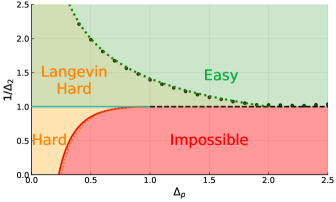
Figure 1: Phase diagram of the spiked $2+3$-spin model (matrix plus order 3 tensor are observed). In the easy (green) region AMP achieves the optimal error smaller than random pick from the prior. In the impossible region (red) the optimal error is as bad as random pick from the prior, and AMP achieves it as well. In the hard region (orange) the optimal error is low, but AMP does not find an estimator better than random pick from the prior. In the case of Langevin algorithm the performance is strictly worse than that for AMP in the sense that the hard region increases up to line $1/\Delta_{2}^{*}=\max(1,\sqrt{\Delta_{3}/2})$, depicted in green dots. The green circles are obtained by numerical extrapolation of the Langevin state evolution equations.

IV Langevin Algorithm and its Analysis

We now turn to the core of the paper and the analysis of the Langevin algorithm. In statistics, the most commonly used way to compute the Bayes-optimal estimator (3) is to attempt to sample the posterior distribution (2) and use several independent samples to compute the expectation in (3). In order to do that one needs to set up a stochastic dynamics on $x$ that has a stationary measure at long times given by the posterior measure (2). The Langevin algorithm is one of the possibilities (others include notably Monte Carlo Markov chain). The common bottleneck is that the time needed to achieve stationarity can be in general exponential in the system size. In which case the algorithm is practically useless. However, this is not always the case and there are regions in parameter space where one can expect that the relaxation to the posterior measure happens on tractable timescales. Therefore it is crucial to understand where this happens and what are the associated relaxation timescales.

The Langevin algorithm on the hypersphere with Hamiltonian given by Eq. (4) reads

$$\dot{x}_{i}(t)=-\mu(t)x_{i}(t)-\frac{\partial\mathcal{H}}{\partial x_{i}}+\eta_{i}(t)\,,$$ (7)

where $\eta_{i}(t)$ is a zero mean noise term, with $\langle\eta_{i}(t)\eta_{j}(t^{\prime})\rangle=2\delta_{ij}\delta(t-t^{\prime})$ where the average $\langle\cdot\rangle$ is with respect to the realizations of the noise. The Lagrange multiplier $\mu(t)$ is chosen in such a way that the dynamics remains on the hypersphere. In the large $N$-limit one finds $\mu(t)=1-2\mathcal{H}_{2}(t)-p\mathcal{H}_{p}(t)$ where the $\mathcal{H}_{2}(t)$ is the 1st term from (4) evaluated at $x(t)$, and $\mathcal{H}_{p}(t)$ is the value of the 2nd term from (4).

The presented spiked matrix-tensor model falls into the particular class of spherical $2+p$-spin glasses Crisanti and Leuzzi (2004, 2006) for which the performance of the Langevin algorithm can be tracked exactly in the large-$N$ limit via a set of integro-partial differential equations Crisanti et al. (1993); Cugliandolo and Kurchan (1993), beforehand dubbed CHSCK. We call this generalised version of the CHSCK equations Langevin State Evolution (LSE) equations in analogy with the state evolution of AMP.

In order to write the LSE equations, we defined three dynamical correlation functions

$$C_{N}(t,t^{\prime}) \equiv\frac{1}{N}\sum_{i=1}^{N}x_{i}(t)x_{i}(t^{\prime})\,,$$ (8)

$$\overline{C}_{N}(t) \equiv\frac{1}{N}\sum_{i=1}^{N}x_{i}(t)x_{i}^{*}\,,$$ (9)

$$R_{N}(t,t^{\prime}) \equiv\frac{1}{N}\sum_{i=1}^{N}\partial x_{i}(t)/\partial h_{i}(t^{\prime})|_{h_{i}=0}\,,$$ (10)

where $h_{i}$ is a pointwise external field applied at time $t^{\prime}$ to the Hamiltonian as $\mathcal{H}+\sum_{i}h_{i}x_{i}$. We note that the correlation functions defined above depend on the realization of the thermal history (i.e. of the noise $\eta(t)$) and on the disorder (here the matrix $Y$ and tensor $T$). However, in the large-$N$ limit they all concentrate around their averages. We thus define $C(t,t^{\prime})=\lim_{N\to\infty}{\mathbb{E}}_{Y,T}\langle C_{N}(t,t^{\prime})\rangle_{\eta}$ and analogously for $\overline{C}(t)$ and $R(t,t^{\prime})$. Standard field theoretical methods Martin et al. (1973) or dynamical cavity method arguments Mézard et al. (1987) can then be used to obtain a closed set of integro-differential equations for the averaged dynamical correlation functions, describing the average global evolution of the system under the Langevin algorithm. The resulting LSE equations are (see the Appendix for a complete derivation)

$$\begin{split}&\frac{\partial}{\partial t}C(t,t^{\prime})=2R(t^{\prime},t)-\mu(t)C(t,t^{\prime})+Q^{\prime}(\overline{C}(t))\overline{C}(t^{\prime})+\int_{0}^{t}dt^{\prime\prime}R(t,t^{\prime\prime})Q^{\prime\prime}(C(t,t^{\prime\prime}))C(t^{\prime},t^{\prime\prime})+\int_{0}^{t^{\prime}}dt^{\prime\prime}R(t^{\prime},t^{\prime\prime})Q^{\prime}(C(t,t^{\prime\prime}))\,,\\ &\frac{\partial}{\partial t}R(t,t^{\prime})=\delta(t-t^{\prime})-\mu(t)R(t,t^{\prime})+\int_{t^{\prime}}^{t}dt^{\prime\prime}R(t,t^{\prime\prime})Q^{\prime\prime}(C(t,t^{\prime\prime}))R(t^{\prime\prime},t^{\prime})\,,\\ &\frac{\partial}{\partial t}\overline{C}(t)=-\mu(t)\overline{C}(t)+Q^{\prime}(\overline{C}(t))+\int_{0}^{t}dt^{\prime\prime}R(t,t^{\prime\prime})\overline{C}(t^{\prime\prime})Q^{\prime\prime}(C(t,t^{\prime\prime}))\,,\end{split}$$ (11)

where we have defined $Q(x)=x^{2}/(2\Delta_{2})+x^{p}/(p\Delta_{p})$. The Lagrange multiplier, $\mu(t)$, is fixed by the spherical constraint, through the condition $C(t,t)=1\;\forall t$. Furthermore causality implies that $R(t,t^{\prime})=0$ if $t<t^{\prime}$. Finally the Ito convention on the stochastic equation (7) gives $\forall t\;\lim_{t^{\prime}\rightarrow t^{-}}R(t,t^{\prime})=1$.

V Behavior of the Langevin algorithm

In order to assess the perfomances of the Langevin algorithm and compare it with AMP, we notice that the correlation function $\overline{C}(t)$ is directly related to accuracy of the algorithm. We solve the differential equations (11) numerically along the lines of Kim and Latz (2001); Berthier et al. (2007a), for a detailed procedure see the Appendix Sec. C.1, codes available online at Sarao Mannelli et al. (2018). In Fig. 2 we plot the correlation with the spike $\overline{C}(t)$ as a function of the running time $t$ for $p=3$, fixed $\Delta_{2}=0.7$ and several values of $\Delta_{p}$, we use as initial condition $\overline{C}(t=0)=10^{-4}$. In the inset of the plot we compare it to the same quantity obtained from the state evolution of the AMP algorithm, with the same initial condition.

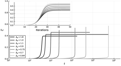
Figure 2: Evolution of the correlation with the signal $\overline{C}(t)$ starting from $\overline{C}(t=0)=10^{-4}$ in the Langevin algorithm at fixed noise on the matrix ($\Delta_{2}=0.7$) and different noises on the tensor ($\Delta_{p}$). As we decrease $\Delta_{p}$ the time required to jump to the solution appears to diverge. Inset: the behavior of $\overline{C}(t)$ as a function of the iteration time for the AMP algorithm for the same values of $\Delta_{p}$ and the same initialization.

For the Langevin algorithm in Fig. 2 we see a pattern that is striking. One would expect that as the noise $\Delta_{p}$ decreases the inference problem is getting easier, the correlation with the signal is larger and is reached sooner in the iteration. This is, after all, exactly what we observe for the AMP algorithm in the inset of Fig. 2. Also for the Langevin algorithm the plateau reached for large times $t$ becomes higher (better accuracy) as the noise $\Delta_{p}$ is reduced. Furthermore the height of the plateau coincides with that reached by AMP, thus testifying the algorithm reached equilibrium. However, contrary to AMP, the relaxation time for the Langevin algorithm increases dramatically when diminishing $\Delta_{p}$ (notice the log scale on x-axes of Fig. 2, as compared to the linear scale of the inset).

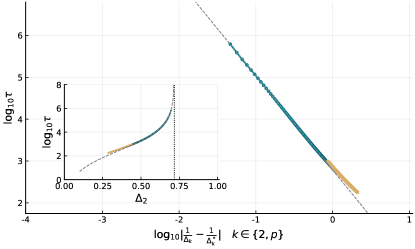
Figure 3: Extrapolation of the Langevin relaxation time. The inset presents the relaxation time for fixed $\Delta_{p}=1$. The main pannel then presents a fit using a power law consistent with a divergence at $\Delta_{2}^{*}\approx 0.72$ The circles are obtained with numerical solution of LSE that uses the dynamical grid while crosses are obtained using a fixed-grid, initial condition was $\overline{C}(t=0)=10^{-40}$ (details in the Appendix).

We define $\tau$ as the time it takes for the correlation to reach a value $\overline{C}_{\rm plateau}/2$. We then plot the value of this equilibration time in the insets of Fig. 3 as a function of the noise $\Delta_{2}$ having fixed $\Delta_{p}$. The data are consistent with a divergence of $\tau$ at a certain finite value of $\Delta^{*}_{2}$. We found that the divergence points are affected by the initial condition of the dynamics $\overline{C}(t=0)$, this aspect is discussed in the Appendix Sec. D.5. In the analysis of the phase diagram we initialize the dynamics to $\overline{C}(t=0)=10^{-40}$ (smaller values have not led to noticeable changes in $\Delta^{*}_{2}$). We calculate the divergence time and we fit the data with a power law $\tau(\Delta)=\left|\frac{1}{\Delta}-\frac{1}{\Delta^{*}}\right|^{-\gamma}$ and we obtain in the particular case of fixed $\Delta_{p}=1.0$ that $\gamma=2.24$ and $\Delta_{2}^{*}=0.72$. We are not able to strictly prove that the divergence of the relaxation time truly occurs, but at least our results imply that for $\Delta_{2}>\Delta_{2}^{*}$ the Langevin algorithm (7) is not a practical solver for the spiked mixed matrix-tensor problem. We will call the region $\Delta_{2}^{*}<\Delta_{2}<1$ where the AMP algorithm works optimally without problems yet Langevin algorithm does not, the Langevin-hard region. $\Delta_{2}^{*}$ is then plotted in Fig. 1 with green points and delimits the Langevin-hard region that extends considerably into the region where the AMP algorithm works optimally in a small number or iterations. Our main conclusion is thus that the Langevin algorithm designed to sample the posterior measure works efficiently in a considerably smaller region of parameters than the AMP as quantified in Fig. 1.

Fig. 4 presents another way to depict the observed data, the correlation $\overline{C}(t)$ reached after time $t$ is plotted as a function of the tensor noise variance $\Delta_{p}$. The results of AMP are depicted with dotted lines and, as one would expect, decrease monotonically as the noise $\Delta_{p}$ increases. The equilibrium value (black dashed) is reached within few dozens of iterations. On the contrary, the correlation reached by the Langevin algorithm after time $t$ is non-monotonic and close to zero for small values of noise $\Delta_{p}$ signaling again a rapidly growing relaxation time when $\Delta_{p}$ is decreased.

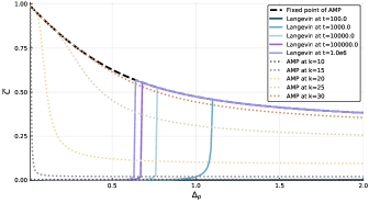
Figure 4: Correlation with the signal of AMP and Langevin at the $k$th iteration (at time $t$) for fixed $\Delta_{2}=0.7$ where both the evolutions start with initial overlap $10^{-4}$.

VI Glassy nature of the Langevin-hard phase

The behaviour of the Langevin dynamics as presented in the last section might seem counter-intuitive at first sight, because one would expect any problem to get simpler when noise $\Delta_{p}$ is decreased. In the present model instead, as $\Delta_{p}$ is decreased, the tensor part of the cost function (4) becomes more important. This brings as a consequence that the landscape becomes rougher and causes the failure of the Langevin algorithm.

In the presence of the hard (for AMP) phase, it was recently argued in Antenucci et al. (2019) that sampling-based algorithms are indeed to be expected to be worse than the approximate message passing ones. This is due to residual glassiness that extends beyond the hard phase. We repeated the analysis of Antenucci et al. (2019) in the present model (details in the Appendix Sec. E) and conclude that while this explanation provides the correct physical picture, the transition line obtained in this way does not agree quantitatively with the numerical extrapolation of the relaxation times we have obtained numerically in the previous section, at least on the timescales on which we were able to solve the LSE equations. The reasons behind this remain open.

In order to obtain a theoretical estimate that quantitatively agrees with the observed behaviour of the LSE, we found the following argument. We first notice that the Langevin dynamics initialized at very small overlap $\overline{C}(t=0)$ remains for a long time at small values of the correlation with the signal. We assume that during this time the dynamics behaves as it would in the mixed $2+p$-spin model without the spike. The model without the spike has been studied extensively in physics literature, precisely with the aim to understand the dynamical properties of glasses Cugliandolo and Kurchan (1993, 1995); Bouchaud et al. (1998). One of the important results of those studies is that the randomly initialized dynamics converges asymptotically to the so-called threshold states. Indeed in Fig. 5 this aspect can be observed in the evolution of the energy. It soon approaches a value that can be evaluated Cugliandolo and Kurchan (1993, 1995); Bouchaud et al. (1998) and corresponds to threshold state energy $E^{\text{\rm th}}$ (horizontal lines)

$$E^{\text{\rm th}}=-Q(1)-\left[\frac{1}{(1-q^{\text{\rm th}})Q^{\prime}(q^{\text{\rm th}})}-\frac{1}{q^{\text{\rm th}}}\right]Q(q^{\text{\rm th}})\;.$$ (12)

In the above equation $q^{\text{\rm th}}$ represents the correlation, a.k.a. overlap, of two configurations randomly picked from the same threshold state, which can be also evaluated as the solution of

$$\frac{1}{1-q^{\text{\rm th}}}=\sqrt{(p-1)\frac{(q^{\text{\rm th}})^{p-2}}{\Delta_{p}}+\frac{1}{\Delta_{2}}}\,.$$ (13)

The derivation of these expressions can be found in Appendix E.1 and in Appendix F. Supported by the numerical results of Fig. 5, we make an approximation that already on the observed time-scales the algorithm converges to the threshold states. The presence of the signal decides whether the algorithm develops a correlation with the signal. To understand how it occurs one has to study the statistical properties of the Thouless-Anderson-Palmer (TAP) free-energy landscape, which is the finite temperature counterpart of the energy landscape, as it has been shown in early days results of spin-glass theory Thouless et al. ; Mézard et al. (1987) and in the recent ones of the mathematical community Chen and Panchenko (2018). The generic picture, that comes out from several years of studies on spin-glass models, is that threshold states corresponds to marginal local minima of the TAP free-energy. Critical points of the TAP free-energy functional that are below the threshold states are typically local minima, while those above are saddles with extensively many negative directions. The threshold states lie in between and have just a few very flat directions. In order to obtain an analytical prediction for the Langevin dynamics threshold, one has to find out how the presence of the spike destabilises the threshold states.

This can be achieved by studying the free-energy Hessian at a threshold state. As shown in App. F, such Hessian reads:

$$\frac{\partial^{2}F}{\partial m_{i}\partial m_{j}}=G_{ij}+\delta_{ij}2\sigma_{F}(q_{th})-\frac{1}{\Delta_{2}}\frac{x_{i}^{*}x_{j}^{*}}{N}+f^{\prime\prime}(q_{th})\frac{m_{i}m_{j}}{N}\,,$$ (14)

where $f^{\prime\prime}(q_{th})$ is positive and its expression can be found in App. F, $m_{i}$ is the average magnetization of site $i$ in the given threshold state, and $G_{ij}$ can be shown to be statistically equivalent to a random matrix having elements which are i.i.d. Gaussian random variables with mean zero and variance

$$\frac{\sigma^{2}_{F}(q_{th})}{N}=\frac{(p-1)q_{th}^{p-2}}{\Delta_{p}}+\frac{1}{\Delta_{2}}\,.$$

The free-energy Hessian evaluated at a typical threshold state is therefore a random matrix belonging to the Gaussian Orthogonal Ensemble plus two rank-one perturbations; one is negative and in the direction of the signal, whereas the other is positive and in the direction of the threshold state.
Results from random matrix theory allow us to completely characterise the spectral properties of the Hessian. Its bulk density of eigenvalues is shifted semi-circle whose left edge touches zero, hence leading to the marginality of the threshold states. For small signal to noise ratio the minimal eigenvalue is zero, whereas when the signal to noise ratio exceeds a certain critical value, the rank-one perturbation in the direction of the signal induces a BBP (Baik, Ben Arous, Peché) transition Edwards and Jones (1976); Baik et al. (2005), where a negative eigenvalue pops out from the Wigner semi-circle, and correspondingly a downward descent direction toward the spike emerges and makes the threshold states unstable. Note that the last term of the Hessian has no effect on the development of an unstable direction as it is positive and uncorrelated with the signal. By adapting the known formulas for the BBP transition to our case, see App. F, we find a landscape-based conjecture for the algorithmic threshold, that is the larger value of $\Delta_{2}^{*}$ between $\Delta_{2}^{*}=1$ and the roots of

$$\Delta_{p}=(p-1)(\Delta^{*}_{2})^{2}(1-\Delta^{*}_{2})^{p-3}\,.$$ (15)

This is the threshold depicted in Fig. 1 for $p=3$ in green dotted line. We note a very good agreement with the data points obtained with extrapolation of the relaxation time from numerical solution of the LSE equations.

In the following, we present a complementary argument that interestingly also makes a direct link with AMP state evolution. We again assume that Langevin dynamics approaches the threshold states. This time we use AMP to determine whether it will remain there or not. If the initial correlation is $0<m^{t=0}\ll 1$ its evolution follows

$$m^{t+1}=(1-q^{\text{\rm th}})\left[\frac{(m^{t})^{p-1}}{\Delta_{p}}+\frac{m^{t}}{\Delta_{2}}\right]\,.$$ (16)

This equation is obtained from the state evolution of the AMP algorithm where the overlap is fixed to $q^{\text{\rm th}}$, as detailed in the Appendix B.3.

The stability condition that decides whether an infinitesimal correlation will grow or decrease under (16) reads $q^{\text{\rm th}}=1-\Delta_{2}$. Using (13), this then leads to eq. (15).

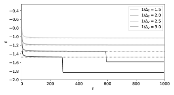
Figure 5: Dynamical evolution of the energy starting from a configuration with overlap $10^{-40}$ at $\Delta_{p}=1.0$ and for various $\Delta_{2}$. The system first tends to the threshold energy, Eq. (12) horizontal lines, and then for sufficiently small $\Delta_{2}$ finds the direction toward the signal.

VII Discussion and Perspectives

Motivated by the general aim to shed light on behaviour and performance of noisy-gradient descent algorithms that are widely used in machine learning, we investigate analytically the performance of the Langevin algorithm in the noisy high-dimensional limit of a spiked matrix-tensor model. We compare it to the performance of the approximate message passing algorithm. While both these algorithms are designed with the aim to sample the posterior measure of the model, we show that the Langevin algorithm fails to find correlation with the signal in a considerable part of the AMP-easy region. Neither of the two algorithm enters the so-called hard phase. Our analysis is based on the Langevin State Evolution equations, generalization of the dynamical theory for mean field spin glasses, that describe the evolution of the algorithm in the large size limit.

The Langevin algorithm performs worse than the AMP due to the underlying glass transition in the corresponding region of parameters. Relying on result from spin glass theory, we present a simple heuristic expression of the Langevin-threshold (15) line which appears to be in agreement with the value obtained from numerical solution of the LSE equations.

We note that so far, in our study of the spiked matrix-tensor model with Langevin dynamics, we only accessed the cost function (4) and its derivatives. We did not allow ourselves to split the cost function in the tensor-related ${\cal H}_{p}$ and the matrix-related ${\cal H}_{2}$ parts. If we did then there is a simple way to overcome the Langevin-hard regime by first considering only the matrix measurements and then slowly turning on the tensor, in a similar way as temperature is tuned in simulated annealing. We study this procedure in the Appendix D.6. It is interesting to underline that from the point of view of Bayesian inference this finding remains somewhat paradoxical. In the setting of this paper we know perfectly the model that generated the data and all its parameters, yet we see that for the Langevin algorithm it is computationally advantageous to mismatch the parameters and perform the annealing in the tensor part in order to reach faster convergence to equilibrium. This is particularly striking given that for AMP it has been proven in Deshpande and Montanari (2015) that mismatching the parameters can never improve the performance. In fact, from a physics point the principle thanks to which AMP does hot share the hurdles of the Langeving algorithm remains an interesting open question.

We stress that the above annealing procedure is a particularity of the present model and will not generalize to a broad range of inference problems, because it is not clear in general how to split the cost function into simple to optimize yet informative part and the rest. A formidably interesting direction for future work consists instead in investigating whether the performance of the Langevin algorithm can be improved in a manner that only accesses the cost function or its derivatives.

While we studied here the spiked matrix-tensor model, we expect that our findings, based on the existence of an underlying glass transition, will hold more universally. We expect them to apply to other local sampling dynamics, e.g. to Monte Carlo Markov chains, and to a broader range of models, e.g. simple models of neural networks. An interesting extension of this work would be to investigate algorithms closer to stochastic gradient descent and models closer to current neural network architectures.

Appendix A Definition of the spiked matrix-tensor model

We consider a teacher-student setting in which the teacher constructs a matrix and a tensor from a randomly sampled signal and the student is asked to recover the signal from the observation of the matrix and tensor provided by the teacher Zdeborová and Krzakala (2016).

The signal, $x^{*}$ is an $N$-dimensional vector whose entries are real i.i.d. random variables sampled from the normal distribution (i.e. the prior is $P_{X}\sim\mathcal{N}(0,1)$). The teacher generates from the signal a symmetric matrix and a symmetric tensor of order $p$. Those two objects are then transmitted through two noisy channels with variances $\Delta_{2}$ and $\Delta_{p}$, so that at the end one has two noisy observations given by

$$Y_{ij}=\frac{x_{i}^{*}x_{j}^{*}}{\sqrt{N}}+\xi_{ij},$$ (17)

$$T_{i_{1},\dots,i_{p}}=\frac{\sqrt{(p-1)!}}{N^{(p-1)/2}}x_{i_{1}}^{*}\dots x_{i_{p}}^{*}+\xi_{i_{1},\dots,i_{p}},$$ (18)

where, for $i<j$ and $i_{1}<\dots<i_{p}$, $\xi_{ij}$ and $\xi_{i_{1},\dots,i_{p}}$ are i.i.d. random variables distributed according to $\xi_{ij}\sim{\cal N}(0,\Delta_{2})$ and $\xi_{i_{1},\dots,i_{p}}\sim{\cal N}(0,\Delta_{p})$. The $\xi_{ij}$ and $\xi_{i_{1},\dots,i_{p}}$ are symmetric random matrix and tensor, respectively. Given $Y_{ij}$ and $T_{i_{1},\dots,i_{p}}$ the inference task is to reconstruct the signal $x^{*}$.

In order to solve this problem we consider the Bayesian approach. This starts from the assumption that both the matrix and tensor have been produced from a process of the same kind of the one described by Eq. (17-18). Furthermore we assume to know the statistical properties of the channel, namely the two variances $\Delta_{2}$ and $\Delta_{p}$, and the prior on $x$. Given this, the posterior probability distribution over the signal is obtained through the Bayes formula

$$P(X|Y,T)=\frac{P(Y,T|X)P(X)}{P(Y,T)}\,,$$ (19)

where

$$\begin{split}P(Y,T|X)&=\prod_{i<j}P_{Y}\left(Y_{ij}\Bigg{|}\frac{x_{i}x_{j}}{\sqrt{N}}\right)\prod_{i_{1}<\dots<i_{p}}P_{T}\left(T_{i_{1}\dots i_{p}}\Bigg{|}\frac{\sqrt{(p-1)!}}{N^{(p-1)/2}}x_{i_{1}}\dots x_{i_{p}}\right)=\\ &\propto\prod_{i<j}e^{-\frac{1}{2\Delta_{2}}\left(Y_{ij}-\frac{x_{i}x_{j}}{\sqrt{N}}\right)^{2}}\prod_{i_{1}<\dots<i_{p}}e^{-\frac{1}{2\Delta_{p}}\left(T_{i_{1}\dots i_{p}}-\frac{\sqrt{(p-1)!}}{N^{(p-1)/2}}x_{i_{1}}\dots x_{i_{p}}\right)^{2}}.\end{split}$$ (20)

Therefore we have

$$\begin{split}P(X|Y,T)&=\frac{1}{Z(Y,T)}\prod_{i}e^{-\frac{1}{2}x_{i}^{2}}\prod_{i<j}e^{-\frac{1}{2\Delta_{2}}\left(Y_{ij}-\frac{x_{i}x_{j}}{\sqrt{N}}\right)^{2}}\prod_{i_{1}<\dots<i_{p}}e^{-\frac{1}{2\Delta_{p}}\left(T_{i_{1}\dots i_{p}}-\frac{\sqrt{(p-1)!}}{N^{(p-1)/2}}x_{i_{1}}\dots x_{i_{p}}\right)^{2}},\end{split}$$ (21)

where $Z(Y,T)$ is a normalization constant.

Plugging Eqs. (17-18) into Eq. (21) allows to rewrite the posterior measure in the form of a Boltzmann distribution of the mixed $2+p$-spin Hamiltonian Crisanti and Leuzzi (2004, 2006, 2013)

$$\begin{split}\mathcal{H}&=-\frac{1}{\Delta_{2}\sqrt{N}}\sum_{i<j}\xi_{ij}x_{i}x_{j}-\frac{\sqrt{(p-1)!}}{\Delta_{p}N^{\frac{p-1}{2}}}\sum_{i_{1}<\dots<i_{p}}\xi_{i_{1}\dots i_{p}}x_{i_{1}}\dots x_{i_{p}}-\frac{N}{2\Delta_{2}}\left(\frac{1}{N}\sum_{i}x_{i}x_{i}^{*}\right)^{2}+\\ &-\frac{N}{p\Delta_{p}}\left(\frac{1}{N}\sum_{i}x_{i}x_{i}^{*}\right)^{p}-\frac{1}{2}\sum_{i=1}^{N}x_{i}^{2}+\text{const.}\end{split}$$ (22)

so that

$$P(X|Y,T)=\frac{1}{\tilde{Z}(Y,T)}e^{-\mathcal{H}}\,.$$ (23)

In the following we will refer to $\tilde{Z}(Y,T)$ as the partition function. We note here that in the large $N$ limit, using a Gaussian prior on the variables $x_{i}$ is equivalent to consider a flat measure over the $N$-dimensional hypersphere $\sum_{i=1}^{N}x_{i}^{2}=N$. This choice will be used when we will describe the Langevin algorithm and in this case the last term in the Hamiltonian will become an irrelevant constant.

Appendix B Approximate Message Passing, state evolution and phase diagrams

Approximate Message Passing (AMP) is a powerful iterative algorithms to compute the local magnetizations $\langle x_{i}\rangle$ given the observed matrix and tensor. It is rooted in the cavity method of statistical physics of disordered systems Thouless et al. (1977); Mézard et al. (1987) and it has been recently developed in the context of statistical inference Donoho et al. (2009), where in the Bayes optimal case it has been conjectured to be optimal among all local iterative algorithms. Among the properties that make AMP extremely useful is the fact that its performances can be analyzed in the thermodynamic limit. Indeed in such limit, its dynamical evolution is described by the so called State Evolution (SE) equations Donoho et al. (2009). In this section we derive the AMP equations and their SE description for the spiked matrix-tensor model and solve them to obtain the phase diagram of the model as a function of the variances $\Delta_{2}$ and $\Delta_{p}$ of the two noisy channels.

B.1 Approximate Message Passing and Bethe free entropy

AMP can be obtained as a relaxed Gaussian closure of the Belief Propagation (BP) algorithm. The derivation that we present follows the same lines of Lesieur et al. (2017a, b). The posterior probability can be represented as a factor graph where all the variables are represented by circles and are linked to squares representing the interactions Mézard and Montanari (2009).

Figure 6: The factor graph representation of the posterior measure of the matrix-tensor factorization model. The variable nodes represented with white circles are the components of the signal while black squares are factor nodes that denote interactions between the variable nodes that appear in the interaction terms of the Boltzmann distribution in Eqs. (22-23). There are three types of factor nodes: $P_{X}$ is the prior that depends on a single variable, $P_{Y}$ that is the probability of observing a matrix element $Y_{ij}$ given the values of the variables $x_{i}$ and $x_{j}$, and finally $P_{T}$ that is the probability of observing a tensor element $T_{i_{1},\dots,i_{p}}$. The posterior, apart from the normalization factor, is simply given by the product of all the factor nodes.

This representation is very convenient to write down the BP equations. In the BP algorithm we iteratively update until convergence a set of variables, which are beliefs of the (cavity) magnetization of the nodes. The intuitive underlying reasoning behind how BP works is the following. Given the current state of the variable nodes, take a factor node and exclude one node among its neighbors. The remaining neighbors through the factor node express a belief on the state of the excluded node. This belief is mathematically described by a probability distribution called message, $\tilde{m}^{t}_{ij\rightarrow i}(x_{i})$ and $\tilde{t}^{t}_{ii_{2}\dots i_{p}\rightarrow i}(x_{i})$ depending on which factor node is selected. At the same time, another belief on the state of the excluded node is given by the rest of the network but the factor node previously taken into account, $m_{i\rightarrow ij}(x_{i})$ and $t_{i\rightarrow ii_{2}\dots i_{p}}(x_{i})$ respectively. All these messages travel in the factor graph carrying partial information on the real magnetization of the single nodes, and they are iterated until convergence. The iterative scheme is described by the following equations

$$\tilde{m}^{t}_{ij\rightarrow i}(x_{i}) \propto\int dx_{j}m^{t}_{j\rightarrow ij}(x_{j})P_{Y}\left(Y_{ij}\Bigg{|}\frac{x_{i}x_{j}}{\sqrt{N}}\right),$$ (24)

$$m^{t+1}_{i\rightarrow ij}(x_{i}) \propto P_{X}(x_{i})\prod_{l\neq j}\tilde{m}^{t}_{il\rightarrow i}(x_{i})\prod_{i_{2}<\dots<i_{p}}\tilde{t}^{t}_{ii_{2}\dots i_{p}\rightarrow i}(x_{i}),$$ (25)

$$\tilde{t}^{t}_{ii_{2}\dots i_{p}\rightarrow i}(x_{i}) \propto\int\prod_{l=2\dots p}\left(dx_{l}t^{t}_{i_{l}\rightarrow ii_{2}\dots i_{p}}(x_{l})\right)P_{T}\left(T_{ii_{2}\dots i_{p}}\Bigg{|}\frac{\sqrt{(p-1)!}}{N^{(p-1)/2}}x_{i}x_{i_{2}}\dots x_{i_{p}}\right),$$ (26)

$$t^{t+1}_{i\rightarrow ii_{2}\dots i_{p}}(x_{i}) \propto P_{X}(x_{i})\prod_{l}\tilde{m}^{t}_{il\rightarrow i}(x_{i})\prod_{k_{2}<\dots<k_{p}\neq i_{2}\dots i_{p}}\tilde{t}^{t}_{ik_{2}\dots k_{p}\rightarrow i}(x_{i})$$ (27)

and we have omitted the normalization constants that guarantee that the messages are probability distributions. When the messages have converged to a fixed point, the estimation of the local magnetizations can be obtained through the computation of the real marginal probability distribution of the variables given by

$$\mu_{i}(x_{i})=\int\left[\prod_{j(\neq i)}dx_{j}\right]P(X|Y,T)=P_{X}(x_{i})\prod_{l}\tilde{m}^{t}_{il\rightarrow i}(x_{i})\prod_{i_{2}<\dots<i_{p}}\tilde{t}^{t}_{ii_{2}\dots i_{p}\rightarrow i}(x_{i})\,.$$ (28)

We note that the computational cost to produce an iteration of BP scales as $O(N^{p})$. Furthermore Eqs. (24 -27) are iterative equations for continuous functions and therefore are extremely hard to solve when dealing with continuous variables. The advantage of AMP is to reduce drastically the computational complexity of the algorithm by closing the equations on a Gaussian ansatz for the messages. This is justified in the present context since the factor graph is fully connected and therefore each iteration step of the algorithm involves sums of a large number of independent random variables that give rise to Gaussian distributions. Gaussian random variables are characterized by their mean and covariance that are readily obtained for $N\gg 1$ expanding the factor nodes for small $\omega_{ij}=x_{i}x_{j}/\sqrt{N}$ and $\omega_{i_{1}\dots i_{p}}=\sqrt{(p-1)!}x_{1}\dots x_{p}/N^{\frac{p-1}{2}}$.

Once the BP equations are relaxed on Gaussian messages, the final step to obtain the AMP algorithm is the so-called TAPyfication procedure Lesieur et al. (2017b); Thouless et al. (1977), which exploits the fact that the procedure of removing one node or one factor produces only a weak perturbation to the real marginals and therefore can be described in terms of the real marginals of the variable nodes themselves. By applying this scheme we obtain the AMP equations, which are described by a set of auxiliary variables $A^{(k)}$ and $B^{(k)}_{i}$ and by the mean $\langle x_{i}\rangle$ and variance $\sigma_{i}=\langle x_{i}^{2}\rangle$ of the marginals of variable nodes. The AMP iterative equations are

$$B^{(2),t}_{i} =\frac{1}{\Delta_{2}\sqrt{N}}\sum_{k}Y_{ki}\hat{x}_{k}^{t}-\frac{1}{\Delta_{2}}\left(\frac{1}{N}\sum_{k}\sigma_{k}^{t}\right)\hat{x}_{i}^{t-1}\,;$$ (29)

$$A^{(2),t} =\frac{1}{\Delta_{2}N}\sum_{k}\left(\hat{x}_{k}^{t}\right)^{2}\,;$$ (30)

$$B^{(p),t}_{i} =\frac{\sqrt{(p-1)!}}{\Delta_{p}N^{(p-1)/2}}\sum_{k_{2}\dots k_{p}}T_{ik_{2}\dots k_{p}}\left(\hat{x}_{k_{2}}^{t}\dots\hat{x}_{k_{p}}^{t}\right)-\frac{p-1}{\Delta_{p}}\left[\left(\frac{1}{N}\sum_{k}\sigma_{k}^{t}\right)\;\left[\frac{1}{N}\sum_{k}\hat{x}_{k}^{t}\hat{x}_{k}^{t-1}\right]^{p-2}\right]\hat{x}_{i}^{t-1}\,;$$ (31)

$$A^{(p),t} =\frac{1}{\Delta_{p}}\left[\frac{1}{N}\sum_{k}\left(\hat{x}_{k}^{t}\right)^{2}\right]^{p-1}\,;$$ (32)

$$\hat{x}_{i}^{t+1} =f(A^{(2)}+A^{(p)},B^{(2)}_{i}+B^{(p)}_{i})\,;$$ (33)

$$\sigma_{i}^{t+1} =\left.\frac{\partial}{\partial B}f(A,B)\right|_{A=A^{(2)}+A^{(p)},B=B^{(2)}_{i}+B^{(p)}_{i}}\,,$$ (34)

$$f(A,B) \equiv\int dx\frac{1}{{\cal Z}(A,B)}xP_{X}(x)e^{Bx-\frac{1}{2}Ax^{2}}=\frac{B}{1+A}\>.$$ (35)

It can be shown that these equations can be obtained as saddle point equations from the so called Bethe free entropy defined as $\Phi_{\text{Bethe}}=\log Z^{\rm Bethe}(Y,T)/N$ where $Z^{\rm Bethe}$ is the Bethe approximation to the partition function which is defined as the normalization of the posterior measure. The expression of the Bethe free entropy per variable can be computed in a standard way (see Mézard and Montanari (2009)) and it is given by

$$\Phi_{\text{Bethe}}=\frac{1}{N}\left(\sum_{i}\log Z_{i}+\sum_{i\leq j}\log Z_{ij}+\sum_{i_{1}\leq\dots\leq i_{p}}\log Z_{i_{1}\dots i_{p}}-\sum_{i(ij)}\log Z_{i,ij}-\sum_{i(ii_{2}\dots i_{p})}\log Z_{i(ii_{2}\dots i_{p})}\right)\;,$$ (36)

where

$$Z_{i}=\int dx_{i}P_{X}(x_{i})\prod_{j}\tilde{m}_{ij\rightarrow i}(x_{i})\prod_{(i_{2}\dots i_{p})}\tilde{t}_{ii_{2}\dots i_{p}\rightarrow i}(x_{i}),$$

$$Z_{ij}=\int\prod_{j(\neq i)}\left[dx_{j}m_{j\rightarrow ij}(x_{j})\right]\prod_{i<j}e^{-\frac{1}{2\Delta_{2}}\left(Y_{ij}-\frac{x_{i}x_{j}}{\sqrt{N}}\right)^{2}}\,,$$

$$Z_{i_{1}\dots i_{p}}=\int\prod_{l=1}^{p}\left[dx_{i_{l}}t_{i_{l}\rightarrow i_{1}\dots i_{p}}(x_{i_{l}})\right]\prod_{i_{1}<\dots<i_{p}}e^{-\frac{1}{2\Delta_{p}}\left(T_{i_{1}\dots i_{p}}-\frac{\sqrt{(p-1)!}}{N^{(p-1)/2}}x_{i_{1}}\dots x_{i_{p}}\right)^{2}}\,,$$

$$Z_{i(ij)}=\int dx_{i}m_{i\rightarrow ij}(x)\tilde{m}_{ij\rightarrow i}(x_{i}),$$

$$Z_{i(ii_{2}\dots i_{p})}=\int dx_{i}t_{i\rightarrow ii_{2}\dots i_{p}}(x)\tilde{t}_{ii_{2}\dots i_{p}\rightarrow i}(x_{i})$$

are a set of normalization factors. Using the Gaussian approximation for the messages and employing the same TAPyification procedure used to get the AMP equations we obtain the Bethe free entropy density as

$$\begin{split}\Phi_{\text{Bethe}}&=\frac{1}{N}\sum_{i}\log{\cal Z}(A^{(p)}+A^{(2)},B^{(p)}_{i}+B^{(2)}_{i})+\frac{p-1}{p}\frac{1}{N}\sum_{i}\Bigg{[}-B_{i}^{(p)}\hat{x}_{i}+A_{i}^{(p)}\frac{\hat{x}_{i}^{2}+\sigma_{i}}{2}\Bigg{]}+\\ &+\frac{p-1}{2p\Delta_{p}}\left(\frac{\sum_{i}\hat{x}_{i}^{2}}{N}\right)^{p-1}\left(\frac{\sum_{i}\sigma_{i}}{N}\right)+\frac{1}{2N}\sum_{i}\Bigg{[}-B_{i}^{(2)}\hat{x}_{i}+A_{i}^{(2)}\frac{\hat{x}_{i}^{2}+\sigma_{i}}{2}\Bigg{]}+\frac{1}{4\Delta_{2}}\left(\frac{\sum_{i}\hat{x}_{i}^{2}}{N}\right)\left(\frac{\sum_{i}\sigma_{i}}{N}\right)\;,\end{split}$$ (37)

where we used the variables defined in eqs. (29-32) for sake of compactness and ${\cal Z}(A,B)$ is defined as

$${\cal Z}(A,B)=\int dxP_{X}(x)e^{Bx-\frac{Ax^{2}}{2}}=\frac{1}{\sqrt{A+1}}e^{\frac{B^{2}}{2(A+1)}}\;.$$ (38)

B.2 Averaged free entropy and its proof

Eq. (37) represents the Bethe free entropy for a single realization of the factor nodes in the large size limit. Here we wish to discuss the actual, exact, value of this free entropy, that is:

$$f_{N}(Y,T)=\frac{\log Z(Y,T)}{N},$$

where the partition function $Z(Y,T)$ is defined as the normalization of the posterior probability distribution, eq. (2). The free entropy is a random variable, since it depends a priori on the planted signal and the noise in the tensor and matrices. However one expects that, since free entropy is an intensive quantity, we expect from the statistical physics intuition that it should be self averaging and concentrate around its mean value in the large $N$ limit Mézard et al. (1987). In fact, this is easily proven. First, since the spherical model has a rotational symmetry, one may assume the planted assignment could be any vector on the hyper-sphere, and we might as well suppose it is the uniform one $x_{i}^{*}=1\forall~{}i$: the true source of fluctuation comes from the noise $Y$ and $T$. These can be controlled by noticing that the free entropy is a Lipshitz function of the Gaussian random variable $Y$ and $T$. Indeed:

$$\partial_{Y_{ij}}f_{N}(Y,T)=\frac{1}{\Delta_{2}N\sqrt{N}}\langle x_{i}x_{j}\rangle$$

, so that the free energy $f_{N}$ is Lipschitz with respect to $Y$ with constant

$$L=\frac{1}{\Delta_{2}N\sqrt{N}}\sqrt{\sum_{i<j}\langle x_{i}x_{j}\rangle^{2}}\leq\frac{1}{\Delta_{2}N\sqrt{N}}\sqrt{\frac{1}{2}\sum_{i,j}\langle x_{i}x_{j}\rangle^{2}}=\frac{1}{\Delta_{2}N\sqrt{N}}\sqrt{\frac{1}{2}\sum_{i,j}\langle x_{i}\tilde{x}_{i}x_{j}\tilde{x}_{j}\rangle}$$

, where $\tilde{x}$ represent a copy (or replica) of the system. In this case

$$L\leq\frac{1}{\Delta_{2}N\sqrt{N}}\sqrt{N^{2}\langle\left(\frac{\sum_{i}x_{i}\tilde{x}_{i}}{N}\right)^{2}\rangle}=\frac{\sqrt{\langle q^{2}\rangle}}{\Delta_{2}\sqrt{N}}$$

, where $q$ is the overlap between the two replica $x$ and $\tilde{x}$, that is bounded by one on the sphere, so $L\leq\frac{1}{\Delta_{2}\sqrt{N}}$. Therefore, by Gaussian concentration of Lipschitz functions (the Tsirelson-Ibragimov-Sudakov inequality Boucheron et al. (2004)), we have for some constant $K$:

$$\textrm{Pr}\left[|f_{n}-\mathbb{E}_{Y}f_{n}|\geq t\right]\leq 2e^{-Nt^{2}/K}\,,$$ (39)

and it particular any fluctuation larger than $O(1/\sqrt{N})$ is (exponentially) rare. A similar computaton shows that $f_{N}$ also concentrates with respect to the tensor $T$. This shows that in the large size limit, we can consider the averaged free entropy:

$${\cal F}_{N}\equiv\frac{1}{N}\mathbb{E}\left[\log Z_{N}\right]$$

.

With our (non-rigorous) statistical physics tools, this can be obtained by averaging Eq. (37) over the disorder, see for instance Lesieur et al. (2017b), and this yields an expression for the free energy called the replica symmetric (RS) formula:

$$\Phi_{\text{RS}}=\lim_{N\to\infty}\mathbb{E}_{Y,T}\frac{\log Z(Y,T)}{N}\,.$$ (40)

We now state precisely the form of $\Phi_{\rm RS}$ and prove the validity of Eq. (40). The RS free entropy for any prior distribution $P_{X}$ reads as

$$\begin{split}\Phi_{\text{RS}}&\equiv{\rm max}_{m}\tilde{\Phi}_{\text{RS}}(m)\quad{\rm where}\\ \tilde{\Phi}_{\text{RS}}(m)&=\mathbb{E}_{W,x^{*}}\left[\log\left[{\cal Z}\left(\frac{m}{\Delta_{2}}+\frac{m^{p-1}}{\Delta_{p}},\left(\frac{m}{\Delta_{2}}+\frac{m^{p-1}}{\Delta_{p}}\right)x^{*}+\sqrt{\frac{m}{\Delta_{2}}+\frac{m^{p-1}}{\Delta_{p}}}W\right)\right]\right]-\frac{1}{4\Delta_{2}}m^{2}-\frac{p-1}{2p\Delta_{p}}m^{p}\;,\end{split}$$ (41)

where $W$ is a Gaussian random variable of zero mean and unit variance and $x^{*}$ is a random variables taken from the prior $P_{X}$. We remind that the function ${\cal Z}(A,B)$ is defined via Eq. (38).

For Gaussian prior $P_{X}$, which is the one of interest here, we obtain

$$\tilde{\Phi}_{\text{RS}}(m)=-\frac{1}{2}\log\left(\frac{m}{\Delta_{2}}+\frac{m^{p-1}}{\Delta_{p}}+1\right)+\frac{1}{2}\left(\frac{m}{\Delta_{2}}+\frac{m^{p-1}}{\Delta_{p}}\right)-\frac{1}{4\Delta_{2}}m^{2}-\frac{p-1}{2p\Delta_{p}}m^{p}\;.$$ (42)

The expression given in the main text is slightly different but can be obtained as follow. First notice that the extremization condition for $\tilde{\Phi}_{\text{RS}}(m)$ reads

$$m=1-\frac{1}{1+\frac{m}{\Delta_{2}}+\frac{m^{p-1}}{\Delta_{p}}}$$ (43)

and by plugging this expression in Eq. (42) we recover the more compact expression $\Phi_{\text{RS}}(m)$ showed in the main text:

$$\Phi_{\text{RS}}(m)=\frac{1}{2}\log\left(1-m\right)+\frac{m}{2}+\frac{m^{2}}{4\Delta_{2}}+\frac{m^{p}}{2p\Delta_{p}}\;.$$ (44)

The two expressions $\Phi_{\text{RS}}(m)$ and $\tilde{\Phi}_{\text{RS}}(m)$ are thus equal for each value of $m$ that satisfy Eq. (43). The parameter $m$ can be interpreted as the average correlation between the true and the estimated signal

$$m=\frac{1}{N}\sum_{i=1}^{N}x_{i}^{*}\hat{x}_{i}\>.$$ (45)

The average minimal mean squared error (MMSE) can be obtained from the maximizer $m$ of the average Bethe free entropy as

$${\rm MMSE}\equiv\frac{1}{N}\sum_{i=1}^{N}\overline{(x_{i}^{*}-\hat{x}_{i})^{2}}=1-m^{*}\,,\quad{\rm where}\quad m^{*}={\rm argmax}\;\tilde{\Phi}_{\text{RS}}(m)\,.$$ (46)

where the overbar stands for the average over the signal $x^{*}$ and the noise of the two Gaussian channels.

The validity of Eq. (41) can be proven rigorously for every prior having a bounded second moment. The proof we shall present is a straightforward generalization of the one presented in Lesieur et al. (2017a) for the pure tensor case, and in Lelarge and Miolane (2016) for the matrix case, and it is based on two main ingredients. The first one is the Guerra interpolation method applied on the Nishimori line Korada and Macris (2009); Krzakala et al. (2016); Lelarge and Miolane (2016), in which we construct an interpolating Hamiltonian that depends on a parameter $t\in[0;1]$ that is used to move from the original Hamiltonian of Eq. (22), to the one corresponding to a scalar denoising problem whose free entropy is given by the first term in Eq. (41). The second ingredient is the Aizenman-Sims-Starr method Aizenman et al. (2003) which is the mathematical version of the cavity method (note that other techniques could also be employed to obtain the same results, see Barbier et al. (2016); Barbier and Macris (2018); Alaoui and Krzakala (2018); Mourrat (2018)). The theorem we want to prove is:

Theorem 1 (Replica-Symmetric formula for the free energy).

Let $P_{X}$ be a probability distribution over  $\mathbb{R}$, with finite second moment $\Sigma_{X}$. Then, for all $\Delta_{2}>0$ and $\Delta_{p}>0$

$${\cal F}_{N}\equiv\frac{1}{N}\mathbb{E}\left[\log Z_{N}\right]\xrightarrow[N\to\infty]{}\sup_{m\geq 0}\tilde{\Phi}_{\rm RS}(m)\equiv\Phi_{\text{\rm RS}}(\Delta_{2},\Delta_{p})\,.$$ (47)

For almost every $\Delta_{2}>0$ and $\Delta_{p}>0$, $\tilde{\Phi}_{\rm RS}$ admits a unique maximizer $m$ over $\mathbb{R}_{+}\times\mathbb{R}_{+}$ and

$${\rm T-MMSE}_{N}\xrightarrow[N\to\infty]{}\Sigma_{X}^{p}-(m^{*})^{p}\,,$$

$${\rm M-MMSE}_{N}\xrightarrow[N\to\infty]{}\Sigma_{X}^{2}-(m^{*})^{2}\,.$$

Here, we have defined the tensor-MMSE $\text{T-MMSE}_{N}$ by the error in reconstructing the tensor:

$$\text{T-MMSE}_{N}(\Delta_{2},\Delta_{p})=\inf_{\hat{\theta}}\left\{\frac{p!}{N^{p}}\sum_{i_{1}<\dots<i_{p}}\left(x^{0}_{i_{1}}\dots x^{0}_{i_{p}}-\hat{\theta}(Y)_{i_{1}\dots i_{p}}\right)^{2}\right\}\,,$$

and the matrix-MMSE $\text{M-MMSE}_{N}$ by the error in reconstructing the matrix:

$$\text{M-MMSE}_{N}(\Delta_{2},\Delta_{p})=\inf_{\hat{\theta}}\left\{\frac{2}{N^{2}}\sum_{i<j}\left(x^{0}_{i}x^{0}_{j}-\hat{\theta}(Y)_{i,j}\right)^{2}\right\}\,,$$

where in both cases the infimum is taken over all measurable functions $\hat{\theta}$ of the observations $Y$.

The result concerning the MMSE is a simple application of the I-MMSE theorem Guo et al. (2005), that relates the derivative of the free energy with respect to the noise variances and the MMSE. The details of the arguments are the same than in the matrix ($p=2$) case (Lelarge and Miolane (2016), corollary 17) and the tensor one (Lesieur et al. (2017a), theorem 2). Indeed, as discussed in Lelarge and Miolane (2016); Lesieur et al. (2017a), these M-MMSE and T-MMSE results implies the vector MMSE result of Eq. (46) when $p$ is odd, and thus in particular for the $p=3$ case discussed in the main text.

Sketch of proof

In this section we give a detailed sketch of the proof theorem $1$. Following the techniques used in many recent works Korada and Macris (2009); Krzakala et al. (2016); Barbier et al. (2016); Lelarge and Miolane (2016); Lesieur et al. (2017a); Barbier and Macris (2018); Alaoui and Krzakala (2018); Barbier et al. (2019), we shall make few technical remarks:

• We will consider only priors with bounded support, $\text{supp}(P_{X})=S\subset[-K;K]$. This allows to switch integrals and derivatives without worries. This condition can then be relaxed to unbounded distributions with bounded second moment using the same techniques as the ones that we are going to present, and the proof is therefore valid in this case. This is detailed for instance in Lelarge and Miolane (2016) sec. 6.2.2.

• Another key ingredient is the introduction of a small perturbation in the model that takes the form of a small amount of side information. This kind of techniques are frequently used in statistical physics, where a small “magnetic field” forces the Gibbs measure to be in a single pure state Georgii (2011). It has also been used in the context of coding theory Macris (2007) for the same reason. In the context of Bayesian inference, we follow the generic scheme proposed by Montanari in Montanari (2008) (see also Coja-Oghlan et al. (2017)) and add a small additional source of information that allows the system to be in a single pure state so that the overlap concentrates on a single value. This source depends on Bernoulli random variables $L_{i}\stackrel{{\scriptstyle\text{i.i.d.}}}{{\sim}}\text{Bern}(\epsilon)$, $i\in[N]$; if $L_{i}=1$, the channel, call it $A$, transmits the correct information. We can then consider the posterior of this new problem, $P(X|A,Y,T)$, and focus on the associated free energy density $F_{N,\epsilon}$ defined as the expected value of the average of the logarithm of normalization constant divided by the number of spins. Then we can immediately prove that for all $N\geq 1$ and $\epsilon,\epsilon^{\prime}\in[0;1]$ it follows: $\left|F_{N,\epsilon}-F_{N,\epsilon^{\prime}}\right|\leq\left(\frac{K^{2p}}{\Delta_{p}}+\frac{K^{4}}{\Delta_{2}}\right)|\epsilon-\epsilon^{\prime}|$. This allows (see for instance Lesieur et al. (2017a)) to obtain the concentration of the posterior distribution around the replica parameter ($q=\frac{1}{N}\langle x^{(1)}\cdot x^{(2)}\rangle$)

  $$\mathbb{E}\left\langle\left(\frac{x^{(1)}\cdot x^{(2)}}{N}-q\right)^{2}\right\rangle\stackrel{{\scriptstyle N\rightarrow\infty}}{{\longrightarrow 0}}\;;$$ (48)

  $$\mathbb{E}\left\langle\left(\frac{x^{*}\cdot x}{N}-q\right)^{2}\right\rangle\stackrel{{\scriptstyle N\rightarrow\infty}}{{\longrightarrow 0}}\;,$$ (49)

  where $x,x^{(1)},x^{(2)}$ are sampled from the posterior distribution and the averages $\langle\cdot\rangle$ and $\mathbb{E}[\cdot]$ are respectively the average over the posterior measure and the remaining random variables.

• Finally, a fundamental property of inference problems which is a direct consequence of the Bayes theorem, and of the fact that we are in the Bayes optimal setting where we know the statistical properties of the signal, namely the prior, and the statistical properties of the channels, namely $\Delta_{2}$ and $\Delta_{p}$, is the so-called Nishimori symmetry Nishimori (2001); Zdeborová and Krzakala (2016): Let $(X,Y)$ be a couple of random variables on a polish space. Let $k\geq 1$ and let $X^{(1)},\dots,X^{(k)}$ be $k$ i.i.d. samples (given $Y$) from the distribution $P(X=\cdot\,|\,Y)$, independently of every other random variables. Let us denote $\langle\cdot\rangle$ the expectation with respect to $P(X=\cdot\,|\,Y)$ and $\mathbb{E}$ the expectation with respect to $(X,Y)$. Then, for all continuous bounded function $f$

  $$\mathbb{E}\langle f(Y,X^{(1)},\dots,X^{(k)})\rangle=\mathbb{E}\langle f(Y,X^{(1)},\dots,X^{(k-1)},X)\rangle\,.$$

  While the consequences of this identity are important, the proof is rather simple: It is equivalent to sample the couple $(X,Y)$ according to its joint distribution or to sample first $Y$ according to its marginal distribution and then to sample $X$ conditionally to $Y$ from its conditional distribution $P(X=\cdot\,|\,Y)$. Thus the $(k+1)$-tuple $(Y,X^{(1)},\dots,X^{(k)})$ is equal in law to $(Y,X^{(1)},\dots,X^{(k-1)},X)$.

The proof of Theorem 1 is obtained by using the Guerra interpolation technique to prove a lower bound for the free entropy and then by applying the Aizenman-Sims-Star scheme to get a matching upper bound.

Lower bound: Guerra interpolation

We now move to the core of the proof. The first part combines the Guerra interpolation method Guerra and Toninelli (2002) developed for matrices in Krzakala et al. (2016) and tensors in Lesieur et al. (2017a).

Consider the interpolating Hamiltonian depending of $t\in[0,1]$

$$\begin{split}\mathcal{H}_{N,t}&=-\sum_{i<j}\left[\frac{\sqrt{t}}{\Delta_{2}\sqrt{N}}Y_{ij}x_{i}x_{j}+\frac{t}{2\Delta_{2}N}(x_{i}x_{j})^{2}\right]+\\ &-\sum_{i_{1}<\dots<i_{p}}\left[\frac{\sqrt{t(p-1)!}}{\Delta_{p}N^{\frac{p-1}{2}}}T_{i_{1}\dots i_{p}}x_{i_{1}}\dots x_{i_{p}}+\frac{t(p-1)!}{2\Delta_{p}N^{p-1}}(x_{i_{1}}\dots x_{i_{p}})^{2}\right]+\\ &-\sum_{j}\left[\sqrt{1-t}\sqrt{\frac{m^{p-1}}{\Delta_{p}}+\frac{m}{\Delta_{2}}}W_{j}x_{j}+(1-t)\left(\frac{m^{p-1}}{\Delta_{p}}+\frac{m}{\Delta_{2}}\right)x_{j}^{*}x_{j}+\frac{1-t}{2}\left(\frac{m^{p-1}}{\Delta_{p}}+\frac{m}{\Delta_{2}}\right)x_{j}^{2}\right]\,,\end{split}$$ (50)

where we have for $t=1$ the regular Hamiltonian and for $t=0$ the first term of Eq. (41) where $W_{j}$ are i.i.d. canonical Gaussian variables. More importantly, for all $t\in[0,1]$ we can show that the Hamiltonian above can be seen as the one emerging for an appropriate inference problem, so that the Nishimori property is kept valid for generic $t\in[0,1]$ Krzakala et al. (2016).

Given the interpolating Hamiltonian we can write the corresponding Gibbs measure,

$$P(x|W,Y,T)=\frac{1}{\mathcal{Z}_{N,t}}P_{X}(x)e^{H_{N,t}(x)}\,,$$ (51)

and the interpolating free entropy

$$\psi_{N}(t)\doteq\frac{1}{N}\mathbb{E}\left[\log\mathcal{Z}_{N,t}\right]\,,$$ (52)

whose boundaries are $\psi_{N}(1)=\frac{1}{N}\mathcal{F}_{N}$ (our target) and $\psi_{N}(0)=\frac{1}{N}\tilde{\Phi}_{\text{RS}}+\frac{1}{4\Delta_{2}}m^{2}+\frac{p-1}{2p\Delta_{p}}m^{p}$. We then use the fundamental theorem of calculus to write

$$\mathcal{F}_{N}=\psi_{N}(1)=\psi_{N}(0)+\frac{1}{N}\underbrace{\mathbb{E}\int_{0}^{1}\left(-\frac{\partial\log\mathcal{Z}_{N,t}}{\partial t}\right)dt}_{\doteq\mathcal{R}}\,.$$ (53)

We work with the second term and use Stein’s lemma which, given a well behaving function $g$, provides the useful relation for a canonical Gaussian variable $Z$: $\mathbb{E}_{Z}[Zg(Z)]=\mathbb{E}_{Z}[g^{\prime}(Z)]$. This yields

$$\begin{split}\mathcal{R}&=-\mathbb{E}\int_{0}^{1}\left[\frac{1}{\mathcal{Z}_{N,t}}\int dx^{N}\frac{\partial\mathcal{H}_{N,t}(x)}{\partial t}P_{X}(x)e^{\mathcal{H}_{N,t}(x)}\right]dt=-\mathbb{E}\int_{0}^{1}\left\langle\frac{\partial\mathcal{H}_{N,t}(x)}{\partial t}\right\rangle dt\\ &=-\mathbb{E}\int_{0}^{1}\left\langle\sum_{i<j}\frac{1}{\Delta_{2}N}(x_{i}^{*}x_{i}x_{j}^{*}x_{j})+\sum_{i_{1}<\dots<i_{p}}\frac{(p-1)!}{\Delta_{2}N^{p-1}}(x_{i_{1}}^{*}x_{i_{1}}\dots x_{i_{p}}^{*}x_{i_{p}})-\sum_{i}\left(\frac{m}{2\Delta_{2}}+\frac{m^{p-1}}{2\Delta_{p}}\right)x_{i}^{*}x_{i}\right\rangle dt\\ &=\mathbb{E}\int_{0}^{1}\left[\frac{1}{4\Delta_{2}}\left\langle\left(\frac{x\cdot x^{*}}{N}\right)^{2}-2m\left(\frac{x\cdot x^{*}}{N}\right)\right\rangle+\frac{1}{2p\Delta_{p}}\left\langle\left(\frac{x\cdot x^{*}}{N}\right)^{p}-pm^{p-1}\left(\frac{x\cdot x^{*}}{N}\right)\right\rangle\right]dt\,.\end{split}$$

where we have used the Nishimori property to replace terms such as $\langle x\rangle^{2}$ by $\langle xx^{*}\rangle$. At this point, we can write

$$\mathcal{R} = \mathbb{E}\int_{0}^{1}\left[\frac{1}{4\Delta_{2}}\left\langle\left(\frac{x\cdot x^{*}}{N}\right)^{2}-2m\left(\frac{x\cdot x^{*}}{N}\right)\right\rangle\right]dt+\mathbb{E}\int_{0}^{1}\left[\frac{1}{2p\Delta_{p}}\left\langle\left(\frac{x\cdot x^{*}}{N}\right)^{p}-pm^{p-1}\left(\frac{x\cdot x^{*}}{N}\right)\right\rangle\right]dt\,$$

$$= -\frac{m^{2}}{4\Delta_{2}}+\frac{1}{4\Delta_{2}}\mathbb{E}\int_{0}^{1}\frac{1}{4\Delta_{2}}\left\langle\left(\frac{x\cdot x^{*}}{N}-m\right)^{2}\right\rangle dt+\frac{1}{2p\Delta_{p}}\mathbb{E}\int_{0}^{1}\ \left\langle\left(\frac{x\cdot x^{*}}{N}\right)^{p}-pm^{p-1}\left(\frac{x\cdot x^{*}}{N}\right)\right\rangle dt\,.$$

The first integral is clearly positive. The second one, however, seems harder to estimate. We may, however, use a simple convexity argument on the function $f(x)=x^{k}$. Indeed observe that $\forall\;a,b\geq 0$ and $p\geq 1$: $a^{p}-pb^{p-1}a\geq(1-p)b^{p}$. We would like to use this property but there is the subtlety that we need $x\cdot x^{*}$ to be non-negative. To bypass this problem we can add again a small perturbation that forces $x\cdot x^{*}$ to concentrate around a non-negative value, without affecting the “interpolating free entropy” $\psi_{N}(t)$ in the $N\to\infty$ limit. This is, again, the argument used in Lesieur et al. (2017a) and originally in Korada and Macris (2009). In this way we can write

$$\mathcal{R} \geq -\frac{m^{2}}{4\Delta_{2}}+\mathbb{E}\int_{0}^{1}\left[\frac{1}{4\Delta_{2}}\left\langle\left(\frac{x\cdot x^{*}}{N}\right)^{2}-2m\left(\frac{x\cdot x^{*}}{N}\right)\right\rangle\right]dt+\frac{(1-p)m^{p}}{4\Delta_{2}}\,$$ (55)

$$\geq -\frac{m^{2}}{4\Delta_{2}}-\frac{(p-1)m^{p}}{4\Delta_{2}}\>.$$

This concludes the proof and yields the lower bound:

$$\mathcal{F}_{N}\geq\psi_{N}(0)-\frac{1}{4\Delta_{2}}m^{2}-\frac{p-1}{2p\Delta_{p}}m^{p}=\frac{1}{N}\tilde{\Phi}_{\text{RS}}(m)\,,$$ (56)

so that for all $m\geq 0$

$$\liminf_{N\to\infty}{\cal F}_{N}=\liminf_{N\to\infty}\psi_{N}(1) =\liminf_{N\to\infty}\left[\psi_{N}(0)+\int_{0}^{1}\psi^{\prime}_{N}(t)dt\right]\geq\tilde{\Phi}_{\rm RS}(m)\,.$$

Upper bound: Aizenman-Sims-Starr scheme.

The matching upper bound is obtained using the Aizenman-Sims-Starr scheme Aizenman et al. (2003) . This is a particularly effective tool that has been already used for these problems, see for example Lelarge and Miolane (2016); Coja-Oghlan et al. (2017); Lesieur et al. (2017a). The method goes as follows. Consider the original system with $N$ variables, $\mathcal{H}_{N}$ and add an new variable $x_{0}$ so that we get an Hamiltonian $\mathcal{H}_{N+1}$. Define the Gibbs measures of the two systems, the first with $N$ variables and the second with $N+1$ variables, and consider the two relative free entropies. Call $A_{N}=\mathbb{E}\left[\log\mathcal{Z}_{N+1}\right]-\mathbb{E}\left[\log\mathcal{Z}_{N}\right]$ their difference. First, we notice that we have $\lim\sup_{N}\mathcal{F}_{N}\leq\lim\sup_{N}A_{N}$ because

$${\cal F}_{N}=\mathbb{E}\frac{1}{N}\log{Z_{N}}=\frac{1}{N}\mathbb{E}\log\left(\frac{Z_{N}}{Z_{N-1}}\frac{Z_{N-1}}{Z_{N-2}}\ldots\frac{Z_{1}}{Z_{0}}\right)=\frac{1}{N}\sum_{i}A_{i}\leq\sup_{i}A_{i}\,.$$

Moreover, we can separate the contribution of the additional variable in the Hamiltonian ${\cal H}_{N+1}$ so that $\mathcal{H}_{N+1}=\tilde{\mathcal{H}}_{N}+x_{0}z(x)+x_{0}^{2}s(x)$, with $x=(x_{1},\dots,x_{N})$, and

$$z(x)=\frac{1}{\sqrt{\Delta_{2}(N+1)}}\sum_{i=1}^{N}Z_{0i}x_{i}+\frac{\sqrt{(p-1)!}}{\sqrt{\Delta_{p}}(N+1)^{(p-1)/2}}\sum_{1\leq i_{1}<\dots<i_{p-1}\leq N}Z_{0i_{1}\dots i_{p-1}}x_{i_{1}}\dots x_{i_{p-1}}+$$

$$\quad+\frac{1}{\Delta_{2}(N+1)}\sum_{i=1}^{N}x_{0}^{*}x_{i}^{*}x_{i}+\frac{(p-1)!}{\Delta_{p}(N+1)^{p-1}}\sum_{1\leq i_{1}<\dots<i_{p-1}\leq N}x_{0}^{*}x_{i_{1}}^{*}x_{i_{1}}\dots x_{i_{p-1}}^{*}x_{i_{p-1}}$$

$$s(x)=-\frac{1}{2\Delta_{2}(N+1)}\sum_{i=1}^{N}x_{i}^{2}-\frac{(p-1)!}{2\Delta_{p}(N+1)^{p-1}}\sum_{1\leq i_{1}<\dots<i_{p-1}\leq N}(x_{i_{1}}\dots x_{i_{p-1}})^{2}$$

and $\mathcal{H}_{N+1}$ is the same expression as Eq. (22) where the $N$ in the denominators are replaced by $N+1$. We rewrite also $\mathcal{H}_{N}(x)$ as a perturbation of $\tilde{\mathcal{H}}_{N}$: $\mathcal{H}_{N}(x)=\tilde{\mathcal{H}}_{N}(x)+y(x)+O(1)$ with

$$y(x)=\frac{1}{\sqrt{\Delta_{2}N}}\sum_{i<j}V_{ij}x_{i}x_{j}+\sqrt{p-1}\frac{\sqrt{(p-1)!}}{\sqrt{\Delta_{p}}N^{p/2}}\sum_{i_{1}<\dots<i_{p}}V_{i_{1}\dots i_{p}}x_{i_{1}}\dots x_{i_{p}}+$$

$$\quad+\frac{1}{N^{2}}\sum_{i<j}\left[x_{i}^{*}x_{i}x_{j}^{*}x_{j}-\frac{1}{2}(x_{i}x_{j})^{2}\right]+(p-1)!\frac{p-1}{N^{p}}\sum_{i_{1}<\dots<i_{p}}\left[x_{i_{1}}^{*}x_{i_{1}}\dots x_{i_{p}}^{*}x_{i_{p}}-\frac{1}{2}(x_{i_{1}}\dots x_{i_{p}})^{2}\right],$$

where the $Z$s and the $V$s are standard Gaussian random variables.

Finally we can observe the partition functions $Z_{N}$ can be interpreted as ensemble averages with respect to $\tilde{\mathcal{H}}_{N}$. Thus $A_{N}=\mathbb{E}\log\left\langle\int P_{X}(x_{0})e^{x_{0}z(x)+x_{0}^{2}s(x)}dx_{0}\right\rangle_{\tilde{\mathcal{H}}_{N}}-\mathbb{E}\log\left\langle e^{y(x)}\right\rangle_{\tilde{\mathcal{H}}_{N}}$. Now, using the Nishimori property and the concentration of the overlap around a non-negative value —that we denote $m(Y,T)$ since it depends explicitly on the disorder— it yields (see Lelarge and Miolane (2016), see section 4.3 for details) (41) in the thermodynamic limit, with $m(Y,T)$ instead of $m$. From this, we can now obtain the upper bound that concludes the proof:

$$\limsup_{N}\mathcal{F}_{N}\leq\limsup_{N}A_{N}\leq\limsup_{N}\mathbb{E}_{Y,T}\tilde{\Phi}_{\text{RS}}[m(Y,T)]\leq\limsup_{N}\sup_{{m}}\Phi_{\text{RS}}({m})\leq\tilde{\Phi}_{\text{RS}}\,.$$ (57)

B.3 State evolution of AMP and its analysis

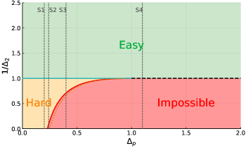
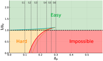
Figure 7: On the left: Phase diagram of the spiked matrix-tensor model for $p=3$. The phase diagram identifies four regions: easy (green), impossible (red), and hard (orange). The lines correspond to different phase transitions namely the stability threshold (dashed black), the information theoretic threshold (solid red), the algorithmic threshold (solid cyan), and the dynamical threshold (dotted orange). The vertical cuts represent the section along which the magnetization is plotted in Fig. 9. On the right: Phase diagram of the spiked matrix-tensor model for $p=4$. The main difference with respect to case $p=3$, is that the algorithmic spinodal (solid cyan) is strictly above the stability threshold (dashed black). The hybrid-hard phase appears between these two lines (combined green and orange color). The vertical cuts represent the section along which the magnetization is plotted in Fig. 10.

The dynamical evolution of the AMP algorithm in the large $N$ limit is described by the so-called State Evolution (SE) equations. The derivation of these equations can be straightforwardly done using the same techniques as developed in Lesieur et al. (2017b). They can be written in terms of two dynamical order parameters namely $m^{t}=\sum_{i}\hat{x}_{i}^{t}x_{i}^{*}/N$, which encodes for the alignment of the current estimation $\hat{x}_{i}^{t}$ of the components of the signal with the signal itself at time $t$ and $q^{t}=\sum_{i}\hat{x}_{i}^{t}\hat{x}_{i}^{t}/N$. Keeping the spherical constraint in mind we obtain the following SE equations

$$\frac{m^{t+1}}{1-q^{t+1}} = \frac{m^{t}}{\Delta_{2}}+\frac{(m^{t})^{p-1}}{\Delta_{p}}\;\;,$$ (58)

$$\frac{q^{t+1}}{(1-q^{t+1})^{2}} = \left[\frac{m^{t}}{\Delta_{2}}+\frac{(m^{t})^{p-1}}{\Delta_{p}}\right]^{2}+\left[\frac{q^{t}}{\Delta_{2}}+\frac{(q^{t})^{p-1}}{\Delta_{p}}\right]\;\;.$$ (59)

Note that eq. (58) at fixed values of $q$ describes the evolution of the parameter $m$, this is why we use in the main text to derive the Langevin threshold eq. (15). Finally, using the Nishimori symmetry it can be shown that $m^{t}=q^{t}$ at all times, see e.g. Zdeborová and Krzakala (2016), and therefore the evolution of the algorithm is characterized by a single order parameter $m^{t}$ whose dynamical evolution is given by

$$m^{t+1}=1-\frac{1}{1+\frac{m^{t}}{\Delta_{2}}+\frac{(m^{t})^{p-1}}{\Delta_{p}}}\;\;.$$ (60)

Note that AMP satisfies the Nishimori property at all times while this condition is violated on the run by the Langevin dynamics. In that case the Nishimori symmetry is recovered only when equilibrium is reached and therefore it is violated when the Langevin algorithm gets trapped in the glass phase, see below. If we initialize the configuration of the estimator $\hat{x}$ at random, the initial value of $m$ will be equal to zero on average. However, finite size fluctuations produce by chance a small bias towards the signal and therefore we consider the initialization to be $m^{t=0}=\epsilon$ being $\epsilon$ an arbitrarily small positive number. We will call $m_{\rm AMP}$ the fixed point of Eq. (60) reached from this infinitesimal initialization. The mean-square-error (MSE) reached by AMP after convergence is then given by ${\rm MSE}_{\rm AMP}=1-m_{\rm AMP}$.

We underline that Eq. (60) can be proven rigorously following Javanmard and Montanari (2013); Richard and Montanari (2014). Finally we note that the fixed point of the SE satisfies the very same Eq. (43) that gives the replica free entropy. In the rest of this section we will study the fixed points of Eq. (60). This will allow too determine the phase diagram of the spiked matrix-tensor model.

We start by observing that $m=0$ is a fixed point of Eq. (60). However, in order to understand whether it is a possible attractor of the AMP dynamics we need to understand its local stability. This can be obtained perturbatively by expanding Eq. (60) around $m=0$

$$m^{t+1}=\frac{m^{t}}{\Delta_{2}}+\left(\frac{m^{t}}{\Delta_{2}}\right)^{2}-\frac{(m^{t})^{p-1}}{\Delta_{p}}+O\left((m^{t})^{3}\right)\;.$$ (61)

It is clear that the non-informative fixed point $m=0$ is stable as long as $\Delta_{2}>1$. We will call $\Delta_{2}=1$ the stability threshold.

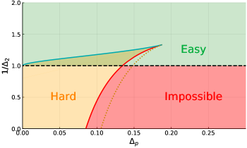
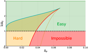
Figure 8: On the left: Phase diagram of the spiked matrix-tensor model for $p=5$. On the right: Phase diagram of the spiked matrix-tensor model for $p=10$. In both cases we observe qualitatively the same scenario found in the right panel of Fig. 7.

When $p=3$ the SE equations are particularly simple and the fixed points are written explicitly as

$$m_{0}=0\,;\quad\quad m_{\pm}=\frac{1}{2}\left[1-\frac{\Delta_{3}}{\Delta_{2}}\pm\sqrt{\left(1+\frac{\Delta_{3}}{\Delta_{2}}\right)^{2}-4\Delta_{3}}\right]\;.$$ (62)

In the regime where $\Delta_{2}>1$, $m_{0}$ and $m_{+}$ are stable while $m_{-}$ in unstable. When $\Delta_{2}$ becomes smaller than one, $m_{+}$ becomes the only non-negative stable solution and therefore $\Delta_{2}=1$ is also known as the algorithmic spinodal since it corresponds to the point where the AMP algorithm converges to the informative fixed point. The informative solution $m_{+}$ exists as long as $\Delta_{2}\leq\Delta^{\rm dyn}_{2}$, where we have defined the dynamical spinodal by

$$\Delta^{\rm dyn}_{2}=\frac{\Delta_{3}}{2\sqrt{\Delta_{3}}-1}\,.$$ (63)

For a generic $p$ we cannot determine the values of the informative fixed points explicitly but we can easily study Eq. (60) numerically to get the full phase diagram.

Furthermore we can obtain the spinodal transition lines as follows. The key observation is that the two spinodals are critical points of the equation $\Delta_{p}(m;\Delta_{2})$ where $\Delta_{2}$ is fixed, or analogously $\Delta_{2}(m;\Delta_{p})$ where $\Delta_{p}$ is fixed (to have a pictorial representation of the idea you can see Fig. 10). We call $x=m/\Delta_{2}+m^{p-1}/\Delta_{p}$, and $f_{\text{SE}}(x)\equiv 1-\frac{1}{1+x}$, then

$$\Delta_{p}\equiv\Delta_{p}(x;\Delta_{2})=\frac{\left(f_{\text{SE}}(x)\right)^{p-1}}{x-\frac{f_{\text{SE}}(x)}{\Delta_{2}}}\;.$$ (64)

Then the stationary points are implicitly defined by

$$0=\frac{d\log\Delta_{p}}{dm}=\frac{\partial\log\Delta_{p}}{\partial x}(1+x)^{2}\propto(p-1)\frac{f_{\text{SE}}^{\prime}(x)}{f_{\text{SE}}(x)}-\frac{1-\frac{f_{\text{SE}}^{\prime}(x)}{\Delta_{2}}}{x-\frac{f_{\text{SE}}^{\prime}(x)}{\Delta_{2}}}=\frac{\frac{2-p}{\Delta_{2}}+(1+x)(p-x-2)}{x(1+x)\left[x+1-\frac{1}{\Delta_{p}}\right]}\;,$$

giving

$$x_{\pm}(\Delta_{2})=\frac{1}{2}\left[p-3\pm\sqrt{(p-1)^{2}-\frac{4}{\Delta_{2}}(p-2)}\right]\;.$$ (65)

Finally $\Delta_{p}\left(x_{\pm}(\Delta_{2});\Delta_{2}\right)$ describes the two spinodals. We can also derive the tri-critical point, when the two spinodals meet, which is given by the zero discriminant condition on (65)

$$\left(\Delta_{p}^{\rm tri};1/\Delta_{2}^{\rm tri}\right)=\left(\frac{4(p-2)\left(\frac{p-3}{p-1}\right)^{p-1}}{(p-3)^{2}};\frac{(p-1)^{2}}{4(p-2)}\right)\;.$$ (66)

B.4 Phase diagrams of spiked matrix-tensor model

In this section we present the phase diagrams for the spiked matrix-tensor model as a function of the two noise levels $\Delta_{2}$ and $\Delta_{p}$ and for several values of $p$. These phase diagrams are plotted in Figs. 7 and 8.

Generically we can have four regions:

• Easy phase (green), where the MSE obtained through AMP coincides with the MMSE which is better than random sampling of the prior.

• Impossible phase (red), where the MMSE and MSE of AMP coincide and are equal to 1 (meaning that $m^{*}=m_{AMP}$=0).

• Hard phase (orange), where the MMSE is smaller than the MSE obtained from AMP and $m^{*}>m_{\rm AMP}\geq 0$.

• Hybrid-hard phase Ricci-Tersenghi et al. (2019) (mix of green and orange), is a part of the hard phase where the AMP performance is strictly better than random sampling from the prior, but still the MSE obtained this way does not match the MMSE, i.e. $m^{*}>m_{\rm AMP}>0$. The hybrid-hard phase can be found for $p\geq 4$.

All these phases are separated by the following transition lines:

• The stability threshold (dashed black line) at $\Delta_{2}=1$ for all $p$. This corresponds to the point where the uninformative fixed point $m=0$ looses its local stability.

• The information theoretic threshold (solid red line). Here $m^{*}>0$ and the MMSE jumps to a value strictly smaller than one.

• The algorithmic threshold (solid cyan line). This is where the fixed point of AMP jumps to the MMSE$<1$. For $p=3$ this line coincides with a segment of the stability threshold while for $p\geq 4$ it is strictly above.

• The dynamic threshold (dotted orange line). Here the most informative fixed point (the one with largest $m_{\rm AMP}$) disappears.

In Figs. 9, and 10 we plot the evolution of the magnetization $m$, as found through the fixed points of the SE equation, for several fixed values of $\Delta_{p}$ and $p=3$ and $p=4$, respectively. The values of $\Delta_{p}$ are identified by the vertical cuts in the phase diagrams of Fig. 7.

(a) Section S1: $p=3$, $\Delta_{p}=0.2$

(b) Section S2:$p=3$, $\Delta_{p}=0.24$

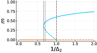
(c) Section S3: $p=3$, $\Delta_{p}=0.4$

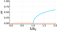
(d) Section S4: $p=3$, $\Delta_{p}=1.1$

Figure 9: Fixed points of Eq. (60) as a function of $\Delta_{2}$ for $p=3$ and several fixed values of $\Delta_{p}$. The values of $\Delta_{p}$ correspond to the vertical cuts in the left panel of Fig. 7. Solid lines are stable fixed point, dashed lines are unstable fixed points. The blue line represent informative fixed points with positive overlap with the signal while the orange line represent a uninformative fixed points with no overlap with the signal. Starting from high $\Delta_{2}$ an informative fixed point appears at the dynamical threshold (vertical dashed line) but is energetically disfavored until the information theoretic threshold (vertical dotted line) and finally it becomes the only stable solution crossing the algorithmic threshold (vertical dotted-dashed line). When the transition is continuous the three vertical threshold lines merge and we have a single second order phase transition, which here occurs at $\Delta_{p}\geq 1$.

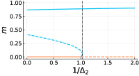
(a) Section S1: $p=4$, $\Delta_{p}=0.1$

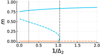
(b) Section S2: $p=4$, $\Delta_{p}=0.14$

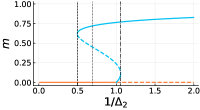
(c) Section S3: $p=4$, $\Delta_{p}=0.18$

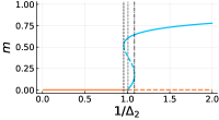
(d) Section S4: $p=4$, $\Delta_{p}=0.24$

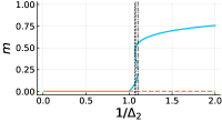
(e) Section S5: $p=4$, $\Delta_{p}=0.27$

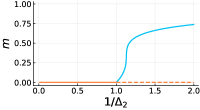
(f) Section S6: $p=4$, $\Delta_{p}=0.3$

Figure 10: Fixed points Eq. (60) as a function of $\Delta_{2}$ for $p=4$ and several fixed values of $\Delta_{p}$. The values of $\Delta_{p}$ correspond to the vertical cuts of the right panel of Fig. 7. The situation is qualitatively similar to Fig. 9, the difference being only the presence of the hybrid-hard phase. We can observe that when the transition is discontinuous, figure from (a) to (e), for $1/\Delta_{2}>1.0$ the uninformative solution becomes unstable and continuously goes to a stable-informative solution which is not the optimal one.

Appendix C Langevin Algorithm and its state evolution

The main goal of our analysis is to compare AMP with the performance of the Langevin dynamics. The advantage of the spiked matrix-tensor model is that in this case the Langevin dynamics can be studied in the large $N$ limit through integro-differential equations for the correlation function, $C(t,t^{\prime})=\lim_{N\to\infty}\sum_{i}\langle x_{i}(t)x_{i}(t^{\prime})\rangle/N$, the response function $R(t,t^{\prime})=\lim_{N\to\infty}\frac{1}{N}\sum_{i}\frac{d\langle x_{i}(t)\rangle}{d\eta_{i}(t^{\prime})}$ and the magnetization $\overline{C}(t)=\lim_{N\to\infty}\sum_{i}\langle x_{i}(t)x_{i}^{*}\rangle/N$.

To obtain these equations we use the techniques developed in the context of mean-field spin glass systems Mézard et al. (1987); Cugliandolo (2003). We call $\eta_{i}(t)$ a time dependent noise and we indicate with $\langle\cdot\rangle$ the average with respect to it. The noise is Gaussian and characterized by $\langle\eta_{i}(t)\rangle=0$ for all $t$ and $i=1,\ldots N$ and $\langle\eta_{i}(t)\eta_{j}(t^{\prime})\rangle=2\delta_{ij}\delta(t-t^{\prime})$. As before we will denote by $\mathbb{E}[\dots]$ the average with respect to the realization of disorder that in this case goes back to the specific realization of the signal.

Before proceeding, it is useful to introduce a set of auxiliary variables that will help in the following. For $k\in\{2,p\}$ we define $r_{k}\equiv r_{k}(t)=2/\left(kT_{k}(t)\Delta_{k}\right)$, $f_{k}(x)=x^{k}/2$ and $m(t)\doteq\frac{1}{N}\sum_{i}x_{i}(t)x_{i}^{*}$, and the random variable $\tilde{\xi}_{i_{1}\dots i_{k}}\equiv\frac{1}{\Delta_{k}}\xi_{i_{1}\dots i_{k}}\sim\mathcal{N}(0,1/\Delta_{k})$. The time dependence in $T_{k}$, will be used in the tensor-annealing protocol that will be used to avoid part of the Langevin hard phase. We introduce a time dependent Hamiltonian

$$\begin{split}\mathcal{H}(t)&=-\frac{1}{T_{2}(t)\sqrt{N}}\sum_{i<j}\tilde{\xi}_{ij}x_{i}(t)x_{j}(t)-\frac{\sqrt{(p-1)}!}{T_{p}(t)N^{\frac{p-1}{2}}}\sum_{i_{1}<\dots<i_{p}}\tilde{\xi}_{i_{1}\dots i_{p}}x_{i_{1}}(t)\dots x_{i_{p}}(t)\\ &-Nr_{2}(t)f_{2}(m(t))-Nr_{p}(t)f_{p}(m(t))\,,\end{split}$$

and the associated Langevin dynamics

$$\begin{split}\dot{x}_{i}(t)&=-\mu(t)x_{i}(t)-\frac{\partial\mathcal{H}}{\partial x_{i}}(t)-\eta_{i}(t)=-\mu(t)x_{i}(t)-\frac{1}{T_{2}(t)\sqrt{N}}\sum_{j(\neq i)}\tilde{\xi}_{ij}x_{j}(t)+\\ &+r_{2}(t)f^{\prime}_{2}(m(t))-\frac{\sqrt{(p-1)!}}{T_{p}(t)N^{\frac{p-1}{2}}}\sum_{(i,i_{1},\dots,i_{p-1})\setminus i}\tilde{\xi}_{ii_{1}\dots i_{p-1}}x_{i_{1}}(t)\cdots x_{i_{p-1}}(t)+r_{p}(t)f^{\prime}_{p}(m(t))-\eta_{i}(t)\,,\end{split}$$ (67)

with $\mu$ a Langrange multiplier that enforces the spherical constraint $\sum_{i=1}^{N}x_{i}^{2}(t)=N$. If $T_{k}(t)=1$ for all $k=2,\ p$, the stationary equilibrium distribution for the Langevin dynamics is given by the posterior measure. Using Ito’s lemma one finds

$$\frac{1}{N}\frac{d}{dt}\sum_{i}x_{i}^{2}(t)=\frac{2}{N}\sum_{i}x_{i}(t)\dot{x}_{i}(t)+2\,.$$

Since the spherical constraint imposes the left-hand-side to be zero, one obtains a condition on the right-hand-side. By plugging the expression (67) in it, one gets that in the large $N$ limit

$$\mu(t)=1-2\mathcal{H}_{2}(t)-p\mathcal{H}_{p}(t)$$ (68)

where

$${\cal H}_{k}=-\frac{\sqrt{(k-1)}!}{T_{k}(t)N^{\frac{k-1}{2}}}\sum_{i_{1}<\dots<i_{k}}\tilde{\xi}_{i_{1}\dots i_{k}}x_{i_{1}}(t)\dots x_{i_{k}}(t)-Nr_{k}(t)f_{k}(m(t))\ \ \ \ \ \ k=2,p$$ (69)

are the parts of the Hamiltonian defined in Eq. (C) relative to the matrix ($k=2$) and to the tensor ($k=p$).

Note that we have not specified any initial condition for the variables $x_{i}(t=0)$. Therefore, since we always employ the spherical constraint, the initial condition for the dynamics is a point on the $N$ dimensional hypersphere $|x|^{2}=N$ extracted with the flat measure.

In order to analyze the Langevin dynamics in the large $N$ limit, we will use the dynamical cavity method Mézard et al. (1987); Castellani and Cavagna (2005); Agoritsas et al. (2018). We will consider a system of $N$ variables, with $N\gg 1$, and add a new one. This new variable will be considered as a small perturbation to the original system but at the same time will be treated self consistently.

C.1 Dynamical Mean-Field Equations

In the following we will drop the time dependence for simplicity restoring it only when it is needed. Given the system with $N$ variables $i=1\dots N$, we add a new one, say $i=0$, and define $\tilde{m}=\frac{1}{N+1}\sum_{i=0}^{N}x_{i}x_{i}^{*}\simeq\frac{1}{N}\sum_{i=0}^{N}x_{i}x_{i}^{*}$ (henceforth we use the symbol $\simeq$ to denote two quantities that are equal up to terms that vanish in the large-$N$ limit). The Langevin equation associated to the new variable is

$$\begin{split}\dot{x}_{0}&=-\mu x_{0}-\frac{1}{T_{2}(t)\sqrt{N}}\sum_{j(\neq 0)}\tilde{\xi}_{0j}x_{j}+r_{2}f^{\prime}_{2}(\tilde{m})-\frac{\sqrt{(p-1)!}}{T_{p}(t)N^{\frac{p-1}{2}}}\sum_{(0,i_{1},\dots,i_{p-1})\setminus 0}\tilde{\xi}_{0i_{1}\dots i_{p-1}}x_{i_{1}}\cdots x_{i_{p-1}}+r_{p}f^{\prime}_{p}(\tilde{m})-\eta_{0}\,,\end{split}$$ (70)

where we used that $N\simeq N+1$ for $N\gg 1$. We will consider the contribution of the new variable on the others in perturbation theory. In the dynamical equations for the variables $i=1,\ldots,N$ we can isolate the variable $i=0$ and write

$$\begin{split}\dot{x}_{i}&=-\mu x_{i}-\frac{1}{T_{2}(t)\sqrt{N}}\sum_{j(\neq i,0)}\tilde{\xi}_{ij}x_{j}+r_{2}f^{\prime}_{2}(m)-\frac{\sqrt{(p-1)!}}{T_{p}(t)N^{\frac{p-1}{2}}}\sum_{(i,i_{1},\dots,i_{p-1})\setminus i,0}\tilde{\xi}_{ii_{1}\dots i_{p-1}}x_{i_{1}}\cdots x_{i_{p-1}}\\ &+r_{p}f^{\prime}_{p}(m)-\eta_{i}+H_{i}\,,\end{split}$$ (71)

with

$$H_{i}(t)=\left(r_{2}f_{2}^{\prime\prime}(m)+r_{p}f_{p}^{\prime\prime}(m)\right)\frac{1}{N}x_{0}-\frac{1}{T_{2}(t)\sqrt{N}}\tilde{\xi}_{0i}x_{0}-\frac{\sqrt{(p-1)!}}{T_{p}(t)N^{\frac{p-1}{2}}}\sum_{(i,0,i_{1},\dots,i_{p-2})\setminus i,0}\tilde{\xi}_{i0i_{1}\dots i_{p-2}}x_{0}x_{i_{1}}\cdots x_{i_{p-2}}\,.$$ (72)

Consider the unperturbed variables $x_{i}^{0}=x_{i}\big{|}_{H_{i}=0}$. At leading order in $N$ we can write

$$x_{i}\simeq x_{i}^{0}+\int_{t_{o}}^{t}dt^{\prime}\frac{\delta x_{i}(t)}{\delta H_{i}(t^{\prime})}\bigg{|}_{H_{i}=0}H_{i}(t^{\prime})\>.$$ (73)

In the dynamical equation for the variable 0 we can identify a piece associated to the unperturbed variables $x_{i}^{0}$. This term can be thought of collectively as a stochastic term $\Xi(t)$

$$\begin{split}\dot{x}_{0}&=-\mu x_{0}\overbrace{-\frac{1}{T_{2}(t)\sqrt{N}}\sum_{j(\neq 0)}\tilde{\xi}_{0j}x^{0}_{j}-\frac{\sqrt{(p-1)!}}{T_{p}(t)N^{\frac{p-1}{2}}}\sum_{(0,i_{1},\dots,i_{p-1})\setminus 0}\tilde{\xi}_{0i_{1}\dots i_{p-1}}x^{0}_{i_{1}}\cdots x^{0}_{i_{p-1}}-\eta_{0}}^{\doteq\;\Xi(t)}+\\ &+r_{2}f^{\prime}_{2}(m)+r_{p}f^{\prime}_{p}(m)+\left(r_{2}f_{2}^{\prime\prime}(m)+r_{p}f_{p}^{\prime\prime}(m)\right)\frac{1}{N}x_{0}-\frac{1}{T_{2}(t)\sqrt{N}}\sum_{j(\neq 0)}\tilde{\xi}_{0j}\int_{t_{o}}^{t}dt^{\prime}\frac{\delta x_{j}(t)}{\delta H_{j}(t^{\prime})}\bigg{|}_{H_{j}=0}H_{j}(t^{\prime})+\\ &-\Bigg{[}\frac{\sqrt{(p-1)!}}{T_{p}(t)N^{\frac{p-1}{2}}}\sum_{(0,i_{1},\dots,i_{p-1})\setminus 0}\tilde{\xi}_{0i_{1}\dots i_{p-1}}\int_{t_{o}}^{t}dt^{\prime}\frac{\delta x_{i_{1}}(t)}{\delta H_{i_{1}}(t^{\prime})}\bigg{|}_{H_{i_{1}}=0}H_{i_{1}}(t^{\prime})x^{0}_{i_{2}}\cdots x^{0}_{i_{p-1}}+\text{permutations}\Bigg{]}\,.\end{split}$$ (74)

Indeed $\Xi(t)$ encodes the effect of a kind of bath made by of the unperturbed variables $i=1,\ldots,N$ to the new one. We can show that at leading order in $N$, $\Xi(t)$ is a Gaussian noise with zero mean and variance given by

$$\begin{split}\mathbb{E}\langle\Xi(t)\Xi(t^{\prime})\rangle&=2\delta(t-t^{\prime})-\mathbb{E}\left[\frac{1}{T_{2}(t)T_{2}(t^{\prime})N}\sum_{j(\neq 0)}\sum_{l(\neq 0)}\tilde{\xi}_{0j}\tilde{\xi}_{0l}x_{j}^{0}(t)x_{l}^{0}(t^{\prime})\right]+\\ &-\mathbb{E}\left[\frac{(p-1)!}{T_{p}(t)T_{p}(t^{\prime})N^{p-1}}\sum_{(0,i_{1},\dots,i_{p-1})\setminus 0}\sum_{(0,j_{1},\dots,j_{p-1})\setminus 0}\tilde{\xi}_{0i_{1}\dots i_{p-1}}\tilde{\xi}_{0j_{1}\dots j_{p-1}}x^{0}_{i_{1}}\cdots x^{0}_{i_{p-1}}x^{0}_{j_{1}}\cdots x^{0}_{j_{p-1}}\right]\end{split}$$

and the second term can be simplified as

$$\begin{split}\mathbb{E}\Bigg{[}&\frac{(p-1)!}{T_{p}(t)T_{p}(t^{\prime})N^{p-1}}\sum_{(0,i_{1},\dots,i_{p-1})\setminus 0}\sum_{(0,j_{1},\dots,j_{p-1})\setminus 0}\tilde{\xi}_{0i_{1}\dots i_{p-1}}\tilde{\xi}_{0j_{1}\dots j_{p-1}}x^{0}_{i_{1}}\cdots x^{0}_{i_{p-1}}x^{0}_{j_{1}}\cdots x^{0}_{j_{p-1}}\Bigg{]}=\\ &\simeq\frac{(p-1)!}{N^{p-1}}\frac{1}{T_{p}(t)T_{p}(t^{\prime})\Delta_{p}}\sum_{(0,i_{1},\dots,i_{p-1})\setminus 0}\langle x^{0}_{i_{1}}(t)x^{0}_{i_{1}}(t^{\prime})\cdots x^{0}_{i_{p-1}}(t)x^{0}_{i_{p-1}}(t^{\prime})\rangle=\frac{1}{T_{p}(t)T_{p}(t^{\prime})\Delta_{p}}C^{p-1}(t,t^{\prime})\,,\end{split}$$

where we used $\sum_{(i_{1},\dots,i_{k})}=\frac{1}{k!}\sum_{1\leq i_{1},\dots,i_{k}\leq N}$, we neglected terms sub-leading in $N$, and we used the definition of the dynamical correlation function

$$C(t,t^{\prime})=\frac{1}{N}\sum_{i=1}^{N}\langle x_{i}(t)x_{i}(t^{\prime})\rangle\>.$$

Therefore we have

$$\mathbb{E}\langle\Xi(t)\rangle=0\,;$$ (75)

$$\mathbb{E}\langle\Xi(t)\Xi(t^{\prime})\rangle=2\delta(t-t^{\prime})+\frac{1}{T_{2}(t)T_{2}(t^{\prime})}C(t,t^{\prime})+\frac{1}{T_{p}(t)T_{p}(t^{\prime})\Delta_{p}}C^{p-1}(t,t^{\prime})\,.$$ (76)

Now we can focus of the deterministic term coming from the first order perturbation in (74). Consider just the integral for the $p$-body term, the other will be given by setting $p=2$

$$\begin{split}\frac{\sqrt{(p-1)!}}{T_{p}(t)N^{\frac{p-1}{2}}}&\sum_{(0,i_{1},\dots,i_{p-1})\setminus 0}\tilde{\xi}_{0i_{1}\dots i_{p-1}}\int_{t_{o}}^{t}dt^{\prime}\frac{\delta x_{i_{1}}(t)}{\delta H_{i_{1}}(t^{\prime})}\bigg{|}_{H_{i_{1}}=0}H_{i_{1}}(t^{\prime})x^{0}_{i_{2}}\cdots x^{0}_{i_{p-1}}+\text{permutations}=\\ &\simeq\frac{(p-1)!}{T_{p}(t)N^{p-1}}\sum_{(0,i_{1},\dots,i_{p-1})\setminus 0}\tilde{\xi}^{2}_{0i_{1}\dots i_{p-1}}\int_{t_{o}}^{t}dt^{\prime}\frac{1}{T_{p}(t^{\prime})}\frac{\delta x_{i_{1}}(t)}{\delta H_{i_{1}}(t^{\prime})}\bigg{|}_{H_{i_{1}}=0}x^{0}_{i_{1}}(t)x^{0}_{i_{1}}(t^{\prime})\cdots x^{0}_{i_{p-2}}(t)x^{0}_{i_{p-2}}(t^{\prime})x_{0}(t^{\prime})+\\ &+\text{permutations}\simeq-\frac{p-1}{T_{p}(t)\Delta_{p}}\int_{t_{o}}^{t}dt^{\prime}\frac{1}{T_{p}(t^{\prime})}R(t,t^{\prime})C^{p-2}(t,t^{\prime})x_{0}(t^{\prime})\end{split}$$ (77)

where we have used the definition of the response function

$$R(t,t^{\prime})=\frac{1}{N}\sum_{i=1}^{N}\left\langle\frac{\delta x_{i}(t)}{\delta H_{i}(t^{\prime})}\right\rangle\>.$$

Plugging (77) into (74) we obtain an effective dynamical equation for the new variable in terms of the correlation and response function of the system with $N$ variables

$$\begin{split}\dot{x}_{0}(t)&=-\mu(t)x_{0}(t)+\Xi(t)+r_{p}f_{p}^{\prime}(\overline{C}(t))+r_{2}f_{2}^{\prime}(\overline{C}(t))+\\ &+\frac{p-1}{T_{p}(t)\Delta_{p}}\int_{t_{o}}^{t}dt^{\prime\prime}\frac{1}{T_{p}(t^{\prime\prime})}R(t,t^{\prime\prime})C^{p-2}(t,t^{\prime\prime})x_{0}(t^{\prime\prime})+\frac{1}{T_{2}(t)\Delta_{2}}\int_{t_{o}}^{t}dt^{\prime\prime}\frac{1}{T_{p}(t^{\prime\prime})}R(t,t^{\prime\prime})x_{0}(t^{\prime\prime})\,.\end{split}$$ (78)

In order to close Eq. (78) we need to give the recipe to compute the correlation and response function.

C.2 Integro-differential equations

In order to obtain the final equations for dynamical order parameters we will assume that the new variable $x_{0}$ is a typical one, namely it has the same statistical nature of all the others. Therefore we can assume that

$$\begin{split}C(t,t^{\prime})&\doteq\mathbb{E}\langle x_{0}(t)x_{0}(t^{\prime})\rangle\\ R(t,t^{\prime})&\doteq\mathbb{E}\left\langle\frac{\delta x_{0}(t)}{\delta\Xi(t^{\prime})}\right\rangle\\ \overline{C}(t)&\doteq\mathbb{E}\langle x_{0}(t)x_{0}^{*}\rangle\>.\end{split}$$ (79)

Eqs. (79) give a way to obtain the equation for all the correlation functions. Indeed we can consider Eq. (78), multiply it by $x_{0}(t^{\prime})$, or differentiate it with respect to an external field $h_{0}(t^{\prime})$, or multiply it it by $x_{0}^{*}$ and we can average the results over the disorder and thermal noise. Using the following identity

$$\begin{split}\mathbb{E}\langle\Xi(t)&x_{0}(t^{\prime})\rangle=\int\mathcal{D}\Xi(t)\;\Xi(t)x_{0}(t^{\prime})e^{-\int d\bar{t}d\tilde{t}\Xi(\bar{t})\mathbb{K}^{-1}(\bar{t},\tilde{t})\Xi(\tilde{t})}=\\ &=-\int dt^{\prime\prime}\int\mathcal{D}\Xi(t)\;x_{0}(t^{\prime})\frac{\delta}{\delta\Xi(t^{\prime\prime})}e^{-\int d\bar{t}d\tilde{t}\Xi(\bar{t})\mathbb{K}^{-1}(\bar{t},\tilde{t})\Xi(\tilde{t})}\mathbb{K}(t,t^{\prime\prime})=\\ &=\int dt^{\prime\prime}\mathbb{E}\left\langle\frac{\delta x_{0}(t^{\prime})}{\delta\Xi(t^{\prime\prime})}\mathbb{K}(t,t^{\prime\prime})\right\rangle=\int dt^{\prime\prime}R(t^{\prime},t^{\prime\prime})\mathbb{K}(t,t^{\prime\prime})=\\ &=2R(t^{\prime},t)+\frac{1}{T_{p}(t)\Delta_{p}}\int_{t_{o}}^{t^{\prime}}dt^{\prime\prime}\frac{1}{T_{p}(t^{\prime\prime})}R(t^{\prime},t^{\prime\prime})C^{p-1}(t,t^{\prime\prime})+\frac{1}{T_{2}(t)\Delta_{2}}\int_{t_{o}}^{t^{\prime}}dt^{\prime\prime}\frac{1}{T_{2}(t^{\prime\prime})}R(t^{\prime},t^{\prime\prime})C(t,t^{\prime\prime})\end{split}$$ (80)

we get the following Langevin State Evolution (LSE) equations

$$\begin{split}\frac{\partial}{\partial t}C(t,t^{\prime})&=\mathbb{E}\langle\dot{x}_{0}(t)x_{0}(t^{\prime})\rangle=2R(t^{\prime},t)-\mu(t)C(t,t^{\prime})+r_{p}(t)f_{p}^{\prime}(\overline{C}(t))\overline{C}(t^{\prime})+r_{2}(t)f_{2}^{\prime}(\overline{C}(t))\overline{C}(t^{\prime})+\\ &+(p-1)\frac{1}{T_{p}(t)\Delta_{p}}\int_{t_{o}}^{t}dt^{\prime\prime}\frac{1}{T_{p}(t^{\prime\prime})}R(t,t^{\prime\prime})C^{p-2}(t,t^{\prime\prime})C(t^{\prime},t^{\prime\prime})+\\ &+\frac{1}{T_{p}(t)\Delta_{p}}\int_{t_{o}}^{t^{\prime}}dt^{\prime\prime}\frac{1}{T_{p}(t^{\prime\prime})}R(t^{\prime},t^{\prime\prime})C^{p-1}(t,t^{\prime\prime})+\\ &+\frac{1}{T_{2}(t)\Delta_{2}}\int_{t_{o}}^{t}dt^{\prime\prime}\frac{1}{T_{2}(t^{\prime\prime})}R(t,t^{\prime\prime})C(t^{\prime},t^{\prime\prime})+\frac{1}{T_{2}(t)\Delta_{2}}\int_{t_{o}}^{t^{\prime}}dt^{\prime\prime}\frac{1}{T_{2}(t^{\prime\prime})}R(t^{\prime},t^{\prime\prime})C(t,t^{\prime\prime})\,;\end{split}$$ (81)

$$\begin{split}\frac{\partial}{\partial t}R(t,t^{\prime})&=\mathbb{E}\left\langle\frac{\delta\dot{x}_{0}(t)}{\delta\Xi(t^{\prime})}\right\rangle=\\ &=\delta(t-t^{\prime})-\mu(t)R(t,t^{\prime})+(p-1)\frac{1}{T_{p}(t)\Delta_{p}}\int_{t^{\prime}}^{t}dt^{\prime\prime}\frac{1}{T_{p}(t^{\prime\prime})}R(t,t^{\prime\prime})R(t^{\prime\prime},t^{\prime})C^{p-2}(t,t^{\prime\prime})+\\ &+\frac{1}{T_{2}(t)\Delta_{2}}\int_{t^{\prime}}^{t}dt^{\prime\prime}\frac{1}{T_{2}(t^{\prime\prime})}R(t,t^{\prime\prime})R(t^{\prime\prime},t^{\prime})\,;\end{split}$$ (82)

$$\begin{split}\frac{\partial}{\partial t}\overline{C}(t)&=\mathbb{E}\langle\dot{x}_{0}(t)x^{*}_{0}\rangle=\\ &=-\mu(t)\overline{C}(t)+r_{p}(t)f_{p}^{\prime}(\overline{C}(t))+r_{2}(t)f_{2}^{\prime}(\overline{C}(t))+\\ &+(p-1)\frac{1}{T_{p}(t)\Delta_{p}}\int_{t_{o}}^{t}dt^{\prime\prime}\frac{1}{T_{p}(t^{\prime\prime})}R(t,t^{\prime\prime})C^{p-2}(t,t^{\prime\prime})\overline{C}(t^{\prime\prime})+\frac{1}{T_{2}(t)\Delta_{2}}\int_{t_{o}}^{t}dt^{\prime\prime}\frac{1}{T_{2}(t^{\prime\prime})}R(t,t^{\prime\prime})\overline{C}(t^{\prime\prime})\,;\end{split}$$ (83)

$$\begin{split}\mu(t)&=1+r_{p}(t)f_{p}^{\prime}(\overline{C}(t))\overline{C}(t)+r_{2}(t)f_{2}^{\prime}(\overline{C}(t))\overline{C}(t)+\\ &+p\frac{1}{T_{p}(t)\Delta_{p}}\int_{t_{o}}^{t}dt^{\prime\prime}\frac{1}{T_{p}(t^{\prime\prime})}R(t,t^{\prime\prime})C^{p-1}(t,t^{\prime\prime})+2\frac{1}{T_{2}(t)\Delta_{2}}\int_{t_{o}}^{t}dt^{\prime\prime}\frac{1}{T_{2}(t^{\prime\prime})}R(t,t^{\prime\prime})C(t,t^{\prime\prime})\,.\end{split}$$ (84)

Note that the last equation for $\mu(t)$ is obtained by imposing the spherical constraint $C(t,t)=1\;\forall t$ using the fact that $0=\frac{dC(t,t)}{dt}=\frac{\partial C(t,t^{\prime})}{\partial t}\Big{|}_{t^{\prime}=t}+\frac{\partial C(t^{\prime},t)}{\partial t}\Big{|}_{t^{\prime}=t}$. The boundary conditions of this equations are: $C(t,t)=1$ the spherical constrain, $R(t,t)=0$ which comes from causality in the Itô approach and $R(t,t^{\prime}\to t^{-})=1$. The initial condition for $\overline{C}(0)=\overline{C}_{0}$ is the overlap with the initial configuration with the true signal. If the initial configuration is random, $\overline{C}_{0}=0$ but will have finite size fluctuations, as in the case of AMP. Therefore we can think that $\overline{C}_{0}=\epsilon$ being $\epsilon$ an arbitrary small positive number.

Appendix D Numerical solution of the LSE equations

The dynamical equations (81-82-83-84) were integrated numerically using two schemes:

• fixed time-grid: the derivatives were discretized and integrated according to their causal structure. This method is suited only for short times (up to $500$ time units);

• dynamic time-grid: the step size is doubled after a given number of steps and the equations are solved self-consistently for every waiting-time. This is the approach proposed in Kim and Latz (2001) and described in Appendix C of Berthier et al. (2007b). It allows integration up to very large times (up to $10^{6}$ time units).

The results of these algorithms are concisely reported in the phase diagram shown in the main paper. In what follows we will present the algorithms and a series of investigations that we carried out to check their stability, we will explain the procedure followed to delimit the Langevin hard region, and we will discuss how we can enter into part of that region by choosing a proper annealing protocol. The codes are available online Sarao Mannelli et al. (2018).

D.1 Fixed time-grid $(2+p)$-spin

In this approach time-derivatives and integrals were discretized using $\frac{\partial}{\partial t}f(t,t^{\prime})\simeq\frac{1}{\Delta t}\left[f(t+\Delta t,t^{\prime})-f(t,t^{\prime})\right]$, and the trapezoidal rule for integration $\int_{0}^{t}f(t)dt\simeq\frac{\Delta t}{2}\sum_{l=0}^{t/\Delta t-1}\left[f(l\Delta t)+f((l+1)\Delta t)\right]$. For instance we defined a function for computing the update in the the response function, (82) as follows

$$\begin{split}R(t+\Delta t&,t^{\prime})=R(t,t^{\prime})-\Delta t\,\mu(t)R(t,t^{\prime})+\frac{1}{2}\frac{\Delta t^{2}}{\Delta_{2}}\sum_{l=t^{\prime}/\Delta t}^{t/\Delta t-1}\left[R(t,l\Delta t)R(l\Delta t,t^{\prime})+R(t,(l+1)\Delta t)R((l+1)\Delta t,t^{\prime})\right]+\\ &+(p-1)\frac{\Delta t^{2}}{\Delta_{p}}\sum_{l=t^{\prime}/\Delta t}^{t/\Delta t-1}\left[C^{p-2}(t,l\Delta t)R(t,l\Delta t)R(l\Delta t,t^{\prime})+C^{p-2}(t,(l+1)\Delta t)R(t,(l+1)\Delta t)R((l+1)\Delta t,t^{\prime})\right]\;.\end{split}$$

Analogously we defined the other integrators. A simple causal integration scheme, being careful with the Itô prescription, gives the pseudo-code below.

  $C(0,0)\leftarrow 1$; $R(0,0)\leftarrow 0$; $\overline{C}(0)\leftarrow\overline{C}_{0}$;

  for $t\leq t_{\max}$ do

     $C(t+\Delta t,t+\Delta t)\leftarrow 1$; $R(t+\Delta t,t+\Delta t)\leftarrow 0$;

     $\mu(t)\leftarrow$ compute_mu($C$, $R$, $\overline{C}$, $t$);

     $\overline{C}(t+\Delta t)\leftarrow$ compute_mag($\mu$, $C$, $R$, $\overline{C}$, $t$);

     for $t^{\prime}\leq t$ do

        $C(t+\Delta t,t^{\prime})\leftarrow$ compute_C($\mu$, $C$, $R$, $\overline{C}$, $t$);

        $R(t+\Delta t,t^{\prime})\leftarrow$ compute_R($\mu$, $C$, $R$, $\overline{C}$, $t$);

     end for

     $R(t+\Delta t,t)\leftarrow 1$;

  end for

D.2 Dynamical time-grid $(2+p)$-spin

(a) Memory allocation;

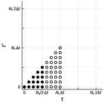
(b) step 1;

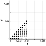
(c) step 2;

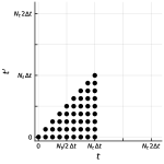
(d) step 3;

(e) step 4.1;

(f) step 4.2;

(g) step 2;

(h) step 3.

Figure 11: Representation of the initialization and the first two iterations for the evaluation of a two-times observable using the dynamic-grid algorithm. The empty circles represent slots allocated in memory but not associated to any specific value, while the full circles are memory slots already associated. For any two time function, it first allocates the memory (a), than it fills half of the grid by linear propagation (b). Still using linear propagation it fills the slots with $t-t^{\prime}\ll 1$ (c), and it sets the other values by imposing self-consistency (d). Finally it halves the grid (e), doubles time step and it allocates the memory (f). Then the algorithm loops following the same scheme as in (b-c-d-e).

The numerical scheme we are going to discuss is presented in the Bayes-optimal case where $T_{2}(t)\equiv T_{p}(t)\equiv 1$. However the derivation that we propose can be easily generalized to the case where the $T$s assume different values, but are constants. Therefore we do not employ this algorithm to solve the LSE equations in the annealing protocol for which instead we use the fixed time-grid algorithm. It is convenient to manipulate the equations to obtain an equivalent set of equations for the functions $C(t,t^{\prime})$, $Q(t,t^{\prime})\doteq 1-C(t,t^{\prime})-\int_{t^{\prime}}^{t}R(t,t^{\prime\prime})dt^{\prime\prime}$, $\overline{C}(t)$, where $Q(t,t^{\prime})$ represents the deviation from Fluctuation Dissipation Theorem (FDT) at time $t$ starting from time $t^{\prime}$. Indeed when the FDT theorem holds, it states that $R(t,t^{\prime})=-\partial_{t}C(t,t^{\prime})$.

We briefly anticipate the strategy that the algorithm uses to solve the equations. The algorithm discretizes the times into $N_{t}$ intervals, first starting from the boundary conditions, $C(t,t)=1$, $Q(t,t)=0$ and $\overline{C}=\overline{C}_{0}\in[0;1]$, it fills the grid for small times (or small time differences $\tau=t-t^{\prime}\ll 1$) using linear propagation. Given a time $t$ and the initial guess for the Lagrange multiplier obtained by the linear propagator, the integrals are discretized and evaluated, then the results is used to update the value of the Lagrange multiplier. This procedure is repeated iteratively until convergence. Once that the first grid is filled, it follows a coarse-graining procedure where the sizes of the time intervals is doubled and only half of the information is retained. This procedure is repeated a fixed number of doubling of the original grid. The doubling scheme allows to explore exponentially long times at the cost of loosing part of the information, the direct consequence of this is the loss of stability for very large times (especially when the functions $C(t,t^{\prime})$, $R(t,t^{\prime})$, $\overline{C}(t)$ undergo fast changes at large times).

Dynamical equations in the algorithm.

We recall the function $f_{k}(x)=\frac{x^{k}}{2}$ and its derivatives, $f_{k}^{\prime}(x)=\frac{kx^{k-1}}{2}$ and $f_{k}^{\prime\prime}(x)=\frac{k(k-1)x^{k-2}}{2}$. For simplicity in the notation, we introduce also $f_{k}(t,t^{\prime})\doteq f_{k}\left(C(t,t^{\prime})\right)$

$$(\partial_{t}+\mu(t))C(t,t^{\prime}) =2R(t^{\prime},t)+r_{2}\overline{C}(t^{\prime})f_{2}^{\prime}(\overline{C}(t))+r_{p}\overline{C}(t^{\prime})f_{p}^{\prime}(\overline{C}(t))+$$

$$+\frac{1}{\Delta_{2}}\int_{0}^{t^{\prime}}dt^{\prime\prime}f_{2}^{\prime}(t,t^{\prime\prime})R(t^{\prime},t^{\prime\prime})+\frac{1}{\Delta_{2}}\int_{0}^{t}dt^{\prime\prime}f_{2}^{\prime\prime}(t,t^{\prime\prime})R(t,t^{\prime\prime})C(t^{\prime},t^{\prime\prime})+$$

$$+\frac{2}{p\Delta_{p}}\int_{0}^{t^{\prime}}dt^{\prime\prime}f_{p}^{\prime}(t,t^{\prime\prime})R(t^{\prime},t^{\prime\prime})+\frac{2}{p\Delta_{p}}\int_{0}^{t}dt^{\prime\prime}f_{p}^{\prime\prime}(t,t^{\prime\prime})R(t,t^{\prime\prime})C(t^{\prime},t^{\prime\prime})\,,$$

$$(\partial_{t}+\mu(t))R(t,t^{\prime}) =\delta(t-t^{\prime})+\frac{1}{\Delta_{2}}\int_{t^{\prime}}^{t}dt^{\prime\prime}f_{2}^{\prime\prime}(t,t^{\prime\prime})R(t,t^{\prime\prime})R(t^{\prime\prime},t^{\prime})+$$

$$+\frac{2}{p\Delta_{p}}\int_{t^{\prime}}^{t}dt^{\prime\prime}f_{p}^{\prime\prime}(t,t^{\prime\prime})R(t,t^{\prime\prime})R(t^{\prime\prime},t^{\prime})\,,$$

$$(\partial_{t}+\mu(t))\overline{C}(t) =r_{2}f_{2}^{\prime}(\overline{C}(t))+r_{p}f_{p}^{\prime}(\overline{C}(t))+$$

$$+\frac{1}{\Delta_{2}}\int_{0}^{t}dt^{\prime\prime}f_{2}^{\prime\prime}(t,t^{\prime\prime})R(t,t^{\prime\prime})\overline{C}(t^{\prime\prime})+\frac{2}{p\Delta_{p}}\int_{0}^{t}dt^{\prime\prime}f_{p}^{\prime\prime}(t,t^{\prime\prime})R(t,t^{\prime\prime})\overline{C}(t^{\prime\prime})\,,$$

$$\mu(t) =1+r_{2}\overline{C}(t)f_{2}^{\prime}(\overline{C}(t))+r_{p}\overline{C}(t)f_{p}^{\prime}(\overline{C}(t))+$$

$$+\frac{2}{\Delta_{2}}\int_{0}^{t}dt^{\prime\prime}f_{2}^{\prime}(t,t^{\prime\prime})R(t,t^{\prime\prime})+\frac{2}{\Delta_{p}}\int_{0}^{t}dt^{\prime\prime}f_{p}^{\prime}(t,t^{\prime\prime})R(t,t^{\prime\prime})\,.$$

Following the lines of Berthier et al. (2007b), we introduce the FDT violation function, $Q(t,t^{\prime})$, and after some manipulation the systems becomes

$$\begin{split}(\partial_{t}+&\mu(t))C(t,t^{\prime})=\overline{C}(t^{\prime})\left[r_{2}f_{2}^{\prime}(\overline{C}(t))+r_{p}f_{p}^{\prime}(\overline{C}(t))\right]+\\ &+\frac{1}{\Delta_{2}}\Big{\{}\int_{0}^{t^{\prime}}dt^{\prime\prime}\left[f_{2}^{\prime}(t,t^{\prime\prime})\frac{\partial Q(t^{\prime},t^{\prime\prime})}{\partial t^{\prime\prime}}+f_{2}^{\prime\prime}(t,t^{\prime\prime})\frac{\partial Q(t,t^{\prime\prime})}{\partial t^{\prime\prime}}C(t^{\prime},t^{\prime\prime})\right]+\\ &-\int_{t^{\prime}}^{t}dt^{\prime\prime}\left[f_{2}^{\prime}(t,t^{\prime\prime})\frac{\partial C(t^{\prime\prime},t^{\prime})}{\partial t^{\prime\prime}}-f_{2}^{\prime\prime}(t,t^{\prime\prime})\frac{\partial Q(t,t^{\prime\prime})}{\partial t^{\prime\prime}}C(t^{\prime\prime},t^{\prime})\right]+f_{2}^{\prime}(1)C(t,t^{\prime})-f_{2}^{\prime}(t,0)C(t^{\prime},0)\Big{\}}+\\ &+\frac{2}{p\Delta_{p}}\Big{\{}\int_{0}^{t^{\prime}}dt^{\prime\prime}\left[f_{p}^{\prime}(t,t^{\prime\prime})\frac{\partial Q(t^{\prime},t^{\prime\prime})}{\partial t^{\prime\prime}}+f_{p}^{\prime\prime}(t,t^{\prime\prime})\frac{\partial Q(t,t^{\prime\prime})}{\partial t^{\prime\prime}}C(t^{\prime},t^{\prime\prime})\right]+\\ &-\int_{t^{\prime}}^{t}dt^{\prime\prime}\left[f_{p}^{\prime}(t,t^{\prime\prime})\frac{\partial C(t^{\prime\prime},t^{\prime})}{\partial t^{\prime\prime}}-f_{p}^{\prime\prime}(t,t^{\prime\prime})\frac{\partial Q(t,t^{\prime\prime})}{\partial t^{\prime\prime}}C(t^{\prime\prime},t^{\prime})\right]+f_{p}^{\prime}(1)C(t,t^{\prime})-f_{p}^{\prime}(t,0)C(t^{\prime},0)\Big{\}}\,,\end{split}$$ (85)

$$\begin{split}(\partial_{t}+&\mu(t))Q(t,t^{\prime})=\mu(t)-1+\frac{1}{\Delta_{2}}\Big{\{}-\int_{t^{\prime}}^{t}dt^{\prime\prime}f_{2}^{\prime}(t,t^{\prime\prime})\frac{\partial Q(t^{\prime\prime},t^{\prime})}{\partial t^{\prime\prime}}+\int_{t^{\prime}}^{t}dt^{\prime\prime}f_{2}^{\prime\prime}(t,t^{\prime\prime})\frac{\partial Q(t,t^{\prime\prime})}{\partial t^{\prime\prime}}[Q(t^{\prime\prime},t^{\prime})-1]+\\ &+f_{2}^{\prime}(1)[Q(t,t^{\prime})-1]+f_{2}^{\prime}(t,0)C(t^{\prime},0)-\int_{0}^{t^{\prime}}dt^{\prime\prime}\left[f_{2}^{\prime}(t,t^{\prime\prime})\frac{\partial Q(t^{\prime},t^{\prime\prime})}{\partial t^{\prime\prime}}+f_{2}^{\prime\prime}(t,t^{\prime\prime})\frac{\partial Q(t,t^{\prime\prime})}{\partial t^{\prime\prime}}C(t^{\prime},t^{\prime\prime})\right]\Big{\}}+\\ &+\frac{2}{p\Delta_{p}}\Big{\{}-\int_{t^{\prime}}^{t}dt^{\prime\prime}f_{p}^{\prime}(t,t^{\prime\prime})\frac{\partial Q(t^{\prime\prime},t^{\prime})}{\partial t^{\prime\prime}}+\int_{t^{\prime}}^{t}dt^{\prime\prime}f_{p}^{\prime\prime}(t,t^{\prime\prime})\frac{\partial Q(t,t^{\prime\prime})}{\partial t^{\prime\prime}}[Q(t^{\prime\prime},t^{\prime})-1]+\\ &+f_{p}^{\prime}(1)[Q(t,t^{\prime})-1]+f_{p}^{\prime}(t,0)C(t^{\prime},0)-\int_{0}^{t^{\prime}}dt^{\prime\prime}\left[f_{p}^{\prime}(t,t^{\prime\prime})\frac{\partial Q(t^{\prime},t^{\prime\prime})}{\partial t^{\prime\prime}}+f_{p}^{\prime\prime}(t,t^{\prime\prime})\frac{\partial Q(t,t^{\prime\prime})}{\partial t^{\prime\prime}}C(t^{\prime},t^{\prime\prime})\right]\Big{\}}+\\ &-\overline{C}(t^{\prime})\left[r_{2}f_{2}^{\prime}(\overline{C}(t))+r_{p}f_{p}^{\prime}(\overline{C}(t))\right]\,,\end{split}$$ (86)

$$\begin{split}(\partial_{t}+&\mu(t))\overline{C}(t)=r_{2}f_{2}^{\prime}(\overline{C}(t))+r_{p}f_{p}^{\prime}(\overline{C}(t))+\frac{1}{\Delta_{2}}\Big{\{}f_{2}^{\prime}(1)\overline{C}(t)-f_{2}^{\prime}(t,0)\overline{C}(0)-\int_{0}^{t}dt^{\prime\prime}f_{2}^{\prime}(t,t^{\prime\prime})\frac{d}{dt^{\prime\prime}}\overline{C}(t^{\prime\prime})+\\ &+\int_{0}^{t}dt^{\prime\prime}f_{2}^{\prime\prime}(t,t^{\prime\prime})\frac{\partial Q(t,t^{\prime\prime})}{\partial t^{\prime\prime}}\overline{C}(t^{\prime\prime})\Big{\}}+\frac{2}{p\Delta_{p}}\Big{\{}f_{p}^{\prime}(1)\overline{C}(t)-f_{p}^{\prime}(t,0)\overline{C}(0)-\int_{0}^{t}dt^{\prime\prime}f_{p}^{\prime}(t,t^{\prime\prime})\frac{d}{dt^{\prime\prime}}\overline{C}(t^{\prime\prime})+\\ &+\int_{0}^{t}dt^{\prime\prime}f_{p}^{\prime\prime}(t,t^{\prime\prime})\frac{\partial Q(t,t^{\prime\prime})}{\partial t^{\prime\prime}}\overline{C}(t^{\prime\prime})\Big{\}}\,,\end{split}$$ (87)

$$\begin{split}\mu(t)&=1+r_{2}\overline{C}(t)f_{2}^{\prime}(\overline{C}(t))+r_{p}\overline{C}(t)f_{p}^{\prime}(\overline{C}(t))+\frac{2}{\Delta_{2}}[f_{2}(1)-f_{2}(t,0)]+\frac{2}{\Delta_{p}}[f_{p}(1)-f_{p}(t,0)]+\\ &+\int_{0}^{t}dt^{\prime\prime}\left[\frac{2}{\Delta_{2}}f_{2}^{\prime}(t,t^{\prime\prime})+\frac{2}{\Delta_{p}}f_{p}^{\prime}(t,t^{\prime\prime})\right]\frac{\partial Q(t,t^{\prime\prime})}{\partial t^{\prime\prime}}\,,\end{split}$$ (88)

further simplifications can be obtained introducing $\mu^{\prime}(t)=\mu(t)-\frac{2}{\Delta_{2}}f_{2}(1)-\frac{2}{\Delta_{p}}f_{p}(1)$

$$\begin{split}\mu^{\prime}(t)&=1+r_{2}\overline{C}(t)f_{2}^{\prime}(\overline{C}(t))+r_{p}\overline{C}(t)f_{p}^{\prime}(\overline{C}(t))-\frac{2}{\Delta_{2}}f_{2}(t,0)-\frac{2}{\Delta_{p}}f_{p}(t,0)+\\ &+\int_{0}^{t}dt^{\prime\prime}\left[\frac{2}{\Delta_{2}}f_{2}^{\prime}(t,t^{\prime\prime})+\frac{2}{\Delta_{p}}f_{p}^{\prime}(t,t^{\prime\prime})\right]\frac{\partial Q(t,t^{\prime\prime})}{\partial t^{\prime\prime}}\,,\end{split}$$ (89)

$$\begin{split}(\partial_{t}+&\mu^{\prime}(t))C(t,t^{\prime})=\overline{C}(t^{\prime})\left[r_{2}f_{2}^{\prime}(\overline{C}(t))+r_{p}f_{p}^{\prime}(\overline{C}(t))\right]+\\ &+\frac{1}{\Delta_{2}}\Big{\{}\int_{0}^{t^{\prime}}dt^{\prime\prime}\left[f_{2}^{\prime}(t,t^{\prime\prime})\frac{\partial Q(t^{\prime},t^{\prime\prime})}{\partial t^{\prime\prime}}+f_{2}^{\prime\prime}(t,t^{\prime\prime})\frac{\partial Q(t,t^{\prime\prime})}{\partial t^{\prime\prime}}C(t^{\prime},t^{\prime\prime})\right]+\\ &-\int_{t^{\prime}}^{t}dt^{\prime\prime}\left[f_{2}^{\prime}(t,t^{\prime\prime})\frac{\partial C(t^{\prime\prime},t^{\prime})}{\partial t^{\prime\prime}}-f_{2}^{\prime\prime}(t,t^{\prime\prime})\frac{\partial Q(t,t^{\prime\prime})}{\partial t^{\prime\prime}}C(t^{\prime\prime},t^{\prime})\right]-f_{2}^{\prime}(t,0)C(t^{\prime},0)\Big{\}}+\\ &+\frac{2}{p\Delta_{p}}\Big{\{}\int_{0}^{t^{\prime}}dt^{\prime\prime}\left[f_{p}^{\prime}(t,t^{\prime\prime})\frac{\partial Q(t^{\prime},t^{\prime\prime})}{\partial t^{\prime\prime}}+f_{p}^{\prime\prime}(t,t^{\prime\prime})\frac{\partial Q(t,t^{\prime\prime})}{\partial t^{\prime\prime}}C(t^{\prime},t^{\prime\prime})\right]+\\ &-\int_{t^{\prime}}^{t}dt^{\prime\prime}\left[f_{p}^{\prime}(t,t^{\prime\prime})\frac{\partial C(t^{\prime\prime},t^{\prime})}{\partial t^{\prime\prime}}-f_{p}^{\prime\prime}(t,t^{\prime\prime})\frac{\partial Q(t,t^{\prime\prime})}{\partial t^{\prime\prime}}C(t^{\prime\prime},t^{\prime})\right]-f_{p}^{\prime}(t,0)C(t^{\prime},0)\Big{\}}\,,\end{split}$$ (90)

$$\begin{split}(\partial_{t}+&\mu^{\prime}(t))Q(t,t^{\prime})=\mu^{\prime}(t)-1-\overline{C}(t^{\prime})\left[r_{2}f_{2}^{\prime}(\overline{C}(t))+r_{p}f_{p}^{\prime}(\overline{C}(t))\right]+\\ &+\frac{1}{\Delta_{2}}\Big{\{}-\int_{t^{\prime}}^{t}dt^{\prime\prime}f_{2}^{\prime}(t,t^{\prime\prime})\frac{\partial Q(t^{\prime\prime},t^{\prime})}{\partial t^{\prime\prime}}+\int_{t^{\prime}}^{t}dt^{\prime\prime}f_{2}^{\prime\prime}(t,t^{\prime\prime})\frac{\partial Q(t,t^{\prime\prime})}{\partial t^{\prime\prime}}[Q(t^{\prime\prime},t^{\prime})-1]+\\ &+f_{2}^{\prime}(t,0)C(t^{\prime},0)-\int_{0}^{t^{\prime}}dt^{\prime\prime}\left[f_{2}^{\prime}(t,t^{\prime\prime})\frac{\partial Q(t^{\prime},t^{\prime\prime})}{\partial t^{\prime\prime}}+f_{2}^{\prime\prime}(t,t^{\prime\prime})\frac{\partial Q(t,t^{\prime\prime})}{\partial t^{\prime\prime}}C(t^{\prime},t^{\prime\prime})\right]\Big{\}}+\\ &+\frac{2}{p\Delta_{p}}\Big{\{}-\int_{t^{\prime}}^{t}dt^{\prime\prime}f_{p}^{\prime}(t,t^{\prime\prime})\frac{\partial Q(t^{\prime\prime},t^{\prime})}{\partial t^{\prime\prime}}+\int_{t^{\prime}}^{t}dt^{\prime\prime}f_{p}^{\prime\prime}(t,t^{\prime\prime})\frac{\partial Q(t,t^{\prime\prime})}{\partial t^{\prime\prime}}[Q(t^{\prime\prime},t^{\prime})-1]+\\ &+f_{p}^{\prime}(t,0)C(t^{\prime},0)-\int_{0}^{t^{\prime}}dt^{\prime\prime}\left[f_{p}^{\prime}(t,t^{\prime\prime})\frac{\partial Q(t^{\prime},t^{\prime\prime})}{\partial t^{\prime\prime}}+f_{p}^{\prime\prime}(t,t^{\prime\prime})\frac{\partial Q(t,t^{\prime\prime})}{\partial t^{\prime\prime}}C(t^{\prime},t^{\prime\prime})\right]\Big{\}}\,,\end{split}$$ (91)

$$\begin{split}(\partial_{t}+&\mu^{\prime}(t))\overline{C}(t)=r_{2}f_{2}^{\prime}(\overline{C}(t))+r_{p}f_{p}^{\prime}(\overline{C}(t))+\frac{1}{\Delta_{2}}\Big{\{}-f_{2}^{\prime}(t,0)\overline{C}(0)+\\ &-\int_{0}^{t}dt^{\prime\prime}f_{2}^{\prime}(t,t^{\prime\prime})\frac{d}{dt^{\prime\prime}}\overline{C}(t^{\prime\prime})+\int_{0}^{t}dt^{\prime\prime}f_{2}^{\prime\prime}(t,t^{\prime\prime})\frac{\partial Q(t,t^{\prime\prime})}{\partial t^{\prime\prime}}\overline{C}(t^{\prime\prime})\Big{\}}+\\ &+\frac{2}{p\Delta_{p}}\Big{\{}-f_{p}^{\prime}(t,0)\overline{C}(0)+\\ &-\int_{0}^{t}dt^{\prime\prime}f_{p}^{\prime}(t,t^{\prime\prime})\frac{d}{dt^{\prime\prime}}\overline{C}(t^{\prime\prime})+\int_{0}^{t}dt^{\prime\prime}f_{p}^{\prime\prime}(t,t^{\prime\prime})\frac{\partial Q(t,t^{\prime\prime})}{\partial t^{\prime\prime}}\overline{C}(t^{\prime\prime})\Big{\}}\,.\end{split}$$ (92)

First order expansion coefficients.

In the numerics we will initialize the grid by a linear propagation of the initial conditions. To determine the coefficients to use we can expand the functions up the second term for small values of $\tau$ (and in the last equation of $t$)

$$\begin{split}C(t^{\prime}+\tau,t^{\prime})&=C(t^{\prime},t^{\prime})+C^{(1,0)}(t^{\prime},t^{\prime})\tau+\frac{1}{2}C^{(2,0)}(t^{\prime},t^{\prime})+O(\tau^{3})\,,\\ Q(t^{\prime}+\tau,t^{\prime})&=Q(t^{\prime},t^{\prime})+Q^{(1,0)}(t^{\prime},t^{\prime})\tau+\frac{1}{2}Q^{(2,0)}(t^{\prime},t^{\prime})+O(\tau^{3})\,,\\ \overline{C}(t)&=\overline{C}(0)+\overline{C}^{(1)}(0)\tau+\frac{1}{2}\overline{C}^{(2)}(0)+O(t^{3})\,.\end{split}$$ (93)

This gives the following coefficients: $C(t,t)=1$, $C^{(1,0)}(t,t)=-1$, $Q(t,t)=0$, $Q^{(1,0)}(t,t)=0$, $\overline{C}(0)=\overline{C}_{0}$ and $\overline{C}^{(1)}(0)=\left[r_{2}f_{2}^{\prime}(\overline{C}_{0})+r_{p}f_{p}^{\prime}(\overline{C}_{0})\right](1-(\overline{C}_{0})^{2})-\overline{C}_{0}$, where $\overline{C}_{0}$ is the initial value of the overlap with the signal.

Numerical integration and derivation.

The set of equations derived above presents six types of integrals

$$I_{ij}^{(1AB)}=\int_{t_{j}}^{t_{i}}dt^{\prime\prime}A(t_{i},t^{\prime\prime})\frac{\partial B(t^{\prime\prime},t_{j})}{\partial t^{\prime\prime}}\,;$$

$$I_{ij}^{(2ABC)}=\int_{t_{j}}^{t_{i}}dt^{\prime\prime}A(t_{i},t^{\prime\prime})\frac{\partial B(t_{i},t^{\prime\prime})}{\partial t^{\prime\prime}}C(t^{\prime\prime},t_{j})\,;$$

$$I_{ij}^{(3AB)}=\int_{0}^{t_{j}}dt^{\prime\prime}A(t_{i},t^{\prime\prime})\frac{\partial B(t_{i},t^{\prime\prime})}{\partial t^{\prime\prime}}\,;$$

$$I_{ij}^{(4ABC)}=\int_{0}^{t_{j}}dt^{\prime\prime}A(t_{i},t^{\prime\prime})\frac{\partial B(t_{i},t^{\prime\prime})}{\partial t^{\prime\prime}}C(t_{j},t^{\prime\prime})\,;$$

$$I_{i}^{(5AB)}=\int_{0}^{t_{i}}dt^{\prime\prime}A(t_{i},t^{\prime\prime})\frac{\partial B(t^{\prime\prime})}{\partial t^{\prime\prime}}\,;$$

$$I_{i}^{(6ABC)}=\int_{0}^{t_{i}}dt^{\prime\prime}A(t_{i},t^{\prime\prime})\frac{\partial B(t_{i},t^{\prime\prime})}{\partial t^{\prime\prime}}C(t^{\prime\prime})\,.$$

The integrals can be easily discretized

$$I_{ij}^{(2ABC)} =\sum_{t_{l}=t_{j}+\delta t}^{t_{i}}\int_{t_{l}-\delta t}^{t_{l}}dt^{\prime\prime}A(t_{i},t^{\prime\prime})\frac{\partial B(t_{i},t^{\prime\prime})}{\partial t^{\prime\prime}}C(t^{\prime\prime},t_{j})\simeq$$

$$\simeq\sum_{t_{l}=t_{j}+\delta t}^{t_{i}}\int_{t_{l}-\delta t}^{t_{l}}dt_{1}A(t_{i},t_{1})\int_{t_{l}-\delta t}^{t_{l}}dt_{2}\frac{\partial B(t_{i},t_{2})}{\partial t_{2}}\int_{t_{l}-\delta t}^{t_{l}}dt_{3}C(t_{3},t_{j})\simeq$$

$$\simeq\sum_{t_{l}=t_{j}+\delta t}^{t_{i}}\frac{1}{2}[A(t_{i},t_{l})+A(t_{i},t_{l}-\delta t)][B(t_{i},t_{l})-B(t_{i},t_{l}-\delta t)]\frac{1}{2}[C(t_{l},t_{j})+C(t_{l}-\delta t,t_{j})]\;.$$

In particular the 6 integrals become

$$\begin{split}&I_{ij}^{(1AB)}=A_{im}B_{mj}-A_{ij}B_{jj}+\sum_{l=m+1}^{i}\frac{1}{2}(A_{il}+A_{i(l-1)})(B_{lj}-B_{(l-1)j})+\\ &\quad\quad\quad-\sum_{l=j+1}^{m}\frac{1}{2}(B_{lj}+B_{(l-1)j})(A_{il}-A_{i(l-1)})=\\ &\quad\quad\quad=A_{im}B_{mj}-A_{ij}B_{jj}+\sum_{l=m+1}^{i}dA_{il}^{(v)}(B_{lj}-B_{(l-1)j})-\sum_{l=j+1}^{m}(A_{il}-A_{i(l-1)})dB_{lj}^{(h)}\,;\end{split}$$ (94)

$$\begin{split}&I_{ij}^{(2ABC)}=\sum_{l=j+1}^{i}\frac{1}{2}(A_{il}+A_{i(l-1)})(B_{lj}-B_{(l-1)j})\frac{1}{2}(C_{lj}+C_{(l-1)j})=\\ &\quad\quad\quad=\sum_{l=m+1}^{i}dA_{il}^{(h)}(B_{il}-B_{i(l-1)})\frac{1}{2}(C_{lj}+C_{(l-1)j})+\sum_{l=j+1}^{m}\frac{1}{2}(A_{il}+A_{i(l-1)})(B_{il}-B_{i(l-1)})dC_{lj}^{(v)}\,;\end{split}$$ (95)

$$I_{ij}^{(3AB)}=A_{ij}B_{jj}-A_{i0}B_{j0}-\sum_{l=1}^{j}(A_{il}-A_{i(l-1)})dB_{jl}^{(v)}\,;$$ (96)

$$I_{ij}^{(4ABC)}=\sum_{l=1}^{j}\frac{1}{2}(A_{il}+A_{i(l-1)})(B_{il}-B_{i(l-1)})dC_{jl}^{(v)}\,;$$ (97)

$$I_{i}^{(5AB)}=\sum_{l=1}^{i}dA_{il}^{(v)}(B_{l}-B_{l-1})\,;$$ (98)

$$I_{i}^{(6ABC)}=\sum_{l=1}^{i}\frac{1}{2}(A_{il}+A_{i(l-1)})(B_{il}-B_{i(l-1)})dC_{l}\,,$$ (99)

where the superscript $(v)$ and $(h)$ represent the vertical ($t^{\prime}$) and horizontal ($t$) derivatives in the discretized times, see Fig. 11 for an intuitive understanding.

We also discretized the derivative using the last two time steps

$$\frac{d}{dt}g(t)=\frac{3}{2\delta t}g(t)-\frac{2}{\delta t}g(t-\delta t)+\frac{1}{2\delta t}g(t-2\delta t)+O(\delta t^{3})\,.$$ (100)

Given the time indices $i$ and $j$, we will define and evaluate the following quantities

$$\begin{split}\{&C_{ij},Q_{ij},M2_{ij},N2_{ij},Mp_{ij},Np_{ij},\text{Cbar}_{i},P2_{i},Pp_{i},mu_{i}\}=\\ &=\{C(t_{i},t_{j}),Q(t_{i},t_{j}),f_{2}^{\prime}(C(t_{i},t_{j})),f_{2}^{\prime\prime}(C(t_{i},t_{j})),f_{p}^{\prime}(C(t_{i},t_{j})),f_{p}^{\prime\prime}(C(t_{i},t_{j})),\overline{C}(t_{i}),f_{2}^{\prime}(\overline{C}(t_{i})),f_{p}^{\prime}(\overline{C}(t_{i})),\mu(t_{i})\}\end{split}$$

plus the respective vertical and horizontal derivatives.

Calling $D_{i}=\frac{3}{2dt}+\mu^{\prime}_{i}-\frac{1}{\Delta_{2}}M2_{ii}-\frac{2}{p\Delta_{p}}Mp_{ii}$, the original dynamical equations are integrated as follow

$$\begin{split}C_{ij}D_{i}&=\frac{2}{dt}C_{(i-1)j}-\frac{1}{2dt}C_{(i-2)j}+\text{Cbar}_{j}(r_{2}P2_{i}+r_{p}Pp_{i})+\\ &+\frac{1}{\Delta_{2}}\left(-\dot{I}_{ij}^{(1f_{2}^{\prime}C)}+I_{ij}^{(2f_{2}^{\prime\prime}QC)}+I_{ij}^{(3f_{2}^{\prime}Q)}+I_{ij}^{(4f_{2}^{\prime\prime}QC)}-M2_{i0}C_{j0}\right)+\\ &+\frac{2}{p\Delta_{p}}\left(-\dot{I}_{ij}^{(1f_{p}^{\prime}C)}+I_{ij}^{(2f_{p}^{\prime\prime}QC)}+I_{ij}^{(3f_{p}^{\prime}Q)}+I_{ij}^{(4f_{p}^{\prime\prime}QC)}-Mp_{i0}C_{j0}\right)\,,\end{split}$$ (101)

$$\begin{split}Q_{ij}D_{i}&=\mu^{\prime}_{i}-1+\frac{2}{dt}Q_{(i-1)j}-\frac{1}{2dt}Q_{(i-2)j}+\text{Cbar}_{j}(r_{2}P2_{i}+r_{p}Pp_{i})+\\ &+\frac{1}{\Delta_{2}}\left(-\dot{I}_{ij}^{(1f_{2}^{\prime}Q)}+I_{ij}^{(2f_{2}^{\prime\prime}Q(Q-1))}-I_{ij}^{(3f_{2}^{\prime}Q)}-I_{ij}^{(4f_{2}^{\prime\prime}QC)}-M2_{i0}C_{i0}\right)+\\ &+\frac{2}{p\Delta_{p}}\left(-\dot{I}_{ij}^{(1f_{p}^{\prime}Q)}+I_{ij}^{(2f_{p}^{\prime\prime}Q(Q-1))}-I_{ij}^{(3f_{p}^{\prime}Q)}-I_{ij}^{(4f_{p}^{\prime\prime}QC)}-Mp_{i0}C_{i0}\right)\,,\end{split}$$ (102)

$$\begin{split}\text{Cbar}_{i}D_{i}&=\frac{2}{dt}\text{Cbar}_{i-1}-\frac{1}{2dt}\text{Cbar}_{i-2}+r_{2}P2_{i}+r_{p}Pp_{i}+\\ &+\frac{1}{\Delta_{2}}\left(-\dot{I}_{i}^{(5f_{2}^{\prime}\text{Cbar})}+I_{i}^{(6f_{2}^{\prime\prime}Q\text{Cbar})}-M2_{i0}\text{Cbar}_{0}\right)+\\ &+\frac{2}{p\Delta_{p}}\left(-\dot{I}_{i}^{(5f_{p}^{\prime}\text{Cbar})}+I_{i}^{(6f_{p}^{\prime\prime}Q\text{Cbar})}-Mp_{i0}\text{Cbar}_{0}\right)\,.\end{split}$$ (103)

In the systems we used $\dot{I}$ to characterize the integrals where we remove from the sum the term present in the left-hand side (e.g. for $C_{ij}$ eq. 101). Using Simpson’s integration formula we define the increments

$$\begin{split}\Delta_{il}&=\frac{1}{12}(Q_{il}-Q_{i(l-1)})\{W_{2}^{2}[-(M2_{i(l+1)}+N2_{i(l+1)}C_{i(l+1)})+8(M2_{il}+N2_{il}C_{il})+5(M2_{i(l-1)}+N2_{i(l-1)}C_{i(l-1)})]+\\ &+W_{p}^{2}[-(Mp_{i(l+1)}+Np_{i(l+1)}C_{i(l+1)})+8(Mp_{il}+Np_{il}C_{il})+5(Mp_{i(l-1)}+Np_{i(l-1)}C_{i(l-1)})]\}\end{split}$$

and we determine $\mu^{\prime}$ as

$$\mu^{\prime}=1+r_{2}P2_{i}+r_{p}Pp_{i}+\delta\mu^{\prime}+\sum_{l=1}^{i-N_{t}/4}\Delta_{il}-(W_{2}^{2}M2_{i0}+W_{p}^{2}Mp_{i0})C_{i0}\,,$$ (104)

with $\delta\mu^{\prime}$ initially set to 0.

Algorithm:

Here we describe the main steps of the algorithm, pictorially represented Fig. 11.

Discretize the time $(t,t^{\prime})$ in $N_{t}$ (even) intervals, the results shown use $N_{t}=1024$.

1. Initialization. Fill the first $N_{t}/2$ times by linear propagation of the value obtained from the perturbative analysis

   $$C_{ij}=1-(i-j)dt\,;$$ (105)

   $$Q_{ij}=0\,;$$ (106)

   $$\text{Cbar}_{i}=\overline{C}_{0}+\left\{\left[r_{2}f_{2}^{\prime}(\overline{C}_{0})+r_{p}f_{p}^{\prime}(\overline{C}_{0})\right](1+(\overline{C}_{0})^{2})-\overline{C}_{0}\right\}dt\,;$$ (107)

   $$M2_{ij}=f_{2}^{\prime}(C_{ij})\,;$$ (108)

   $$N2_{ij}=f_{2}^{\prime\prime}(C_{ij})\,;$$ (109)

   $$Mp_{ij}=f_{p}^{\prime}(C_{ij})\,;$$ (110)

   $$Np_{ij}=f_{p}^{\prime\prime}(C_{ij})\,.$$ (111)

2. Fill the grid (small $\tau$). Continue to propagate the values for small time differences $\tau=t-t^{\prime}\ll 1$. In terms of the algorithm it means that we have some elements of the grid, $N_{c}$ of them, close to the diagonal that will be updated by linear propagation because the approximation of small $\tau$ is still valid. In our simulation the first $\Delta t$ is of the order $10^{-7}$ and $N_{c}=2$.

3. Fill the grid (larger $\tau$). The rest of the values will be copied from the previous $t$ ($A_{t+\Delta t,t^{\prime}}=A_{t,t^{\prime}}$). These values are the initial guess for solving the self-consistent equations (101-102-103) and (104), in this procedure the derivatives are updated using the 2nd order discretization.

4. Half the grid and expand. The grid is decimated which means that each observable is contracted $A_{i,j}\leftarrow A_{2i,2j}$ and the derivate are updated as follows $dA^{(h)}_{i,j}\leftarrow\frac{1}{2}(dA^{(h)}_{2i,2j}+dA^{(h)}_{2i-1,2j})$, $dA^{(v)}_{i,j}\leftarrow\frac{1}{2}(dA^{(v)}_{2i,2j}+dA^{(v)}_{2i,2j-1})$. The new time step is now: $\Delta t\leftarrow 2\Delta t$.

5. Start over from step 2.

D.3 Numerical checks on the dynamical algorithm

The dynamic-grid algorithm has been checked in a variety of ways.

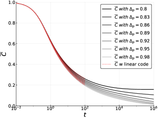
(a) $p=3\quad\Delta_{2}=1.01$

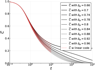
(b) $p=3\quad\Delta_{2}=1.05$

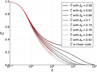
(c) $p=3\quad\Delta_{2}=1.10$

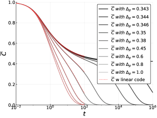
(d) $p=3\quad\Delta_{2}=2.00$

Figure 12: Evolution of the correlation with the signal starting from the solution, $\overline{C}_{0}=1.0$ at fixed $\Delta_{2}$ for different $\Delta_{p}$. The dotted red line overlapping with other lines, is the same quantity evaluated using the fixed grid algorithm up to time $100$. We have started the LSE from an informative initial condition.

Cross-checking using the fixed-grid algorithm.

For short times the dynamical equations were solved using the fixed-grid algorithm and compared with the outcome of the dynamic-grid algorithm, obtaining the same results, see Fig. 12. In the figure we used the fixed-grid with $t_{\max}=100$ and the $\Delta t=6.25*10^{-3}$.

Same magnetization in the easy region.

In the impossible and easy regions, the overlap with the signal of both AMP and dynamic-grid integration, converges to the same value. In Fig. 13 we show the overlap obtained with AMP, black dashed line, and the overlap achieved by the integration scheme at a given time. We can see that the overlap with the signal as obtained solving the LSE equations converges to the same value of the fixed point of AMP. Given a fixed $\Delta_{2}$ we can observe that the time to convergence increase very rapidly as we decrease $\Delta_{p}$. We fitted this increase of the relaxation time to get the boundary of the Langevin hard region.

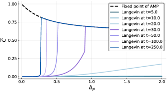
(a) $p=3\quad\Delta_{2}=0.40$

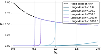
(b) $p=3\quad\Delta_{2}=0.60$

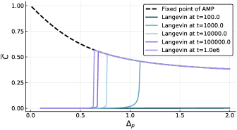
(c) $p=3\quad\Delta_{2}=0.70$

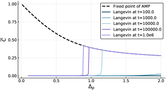
(d) $p=3\quad\Delta_{2}=0.80$

Figure 13: Correlation with the signal of AMP (dotted lines) and Langevin (solid lines) at $k$th iteration and $t$ time respectively starting in both cases with an initial overlap of $10^{-4}$. The black dashed line is the asymptotic value predicted with AMP. In the easy region, provided enough running time, Langevin dynamics finds the same alignment as AMP. The figures show qualitatively the same behaviour for different values of $\Delta_{2}$.

Dynamical transition.

The dynamical transition where the finite magnetization fixed point disappears can be regarded as a clustering or dynamical glass transition. Indeed coming from the impossible phase, going towards the hard phase, at the dynamical transition the free energy landscape changes and the unique ergodic paramagnetic minimum of the impossible phase gets clustered into an exponential number of metastable glassy states (see Sec. E). Correspondingly the relaxation time of the Langevin algorithm diverges. Fitting this divergence with a power law we obtain an alternative estimation of the dynamical line. In the right panel of Fig. 14 we plot with yellow points the dynamical transition line as extracted from the fit of the relaxation time of the Langevin algorithm extracted coming from the impossible phase and entering in the hard phase.

D.4 Extrapolation procedure

In order to determine the Langevin Hard region, given a fixed value of $\Delta_{p}$ ($\Delta_{2}$), we measure the relaxation time that it takes to relax to equilibrium. On approaching the Langevin hard region, this relaxation time increases and we extrapolate the growth to obtain the critical $\Delta_{p}^{*}$ ($\Delta_{2}^{*}$ respectively) where the relaxation time appears to diverge. The extrapolation is done starting from $\overline{C}_{0}=10^{-40}$ and assuming a power law divergence. Fig. 14 shows the results of this procedure for the cases $2+3$ and $2+4$. We remark that the divergence times increase as $p$ increases. Therefor in reason of the instability of the code for large times it becomes difficult to extrapolate the threshold accurately. In particular in the right panel of Fig. 14 when estimating the threshold for $2+4$, we consider horizontal sections and the points extrapolated for $\Delta_{2}$ close to the threshold $\Delta_{2}=1.0$ are very hard to estimate because of these instabilities.

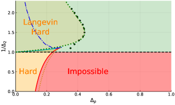
Figure 14: On the left: phase diagram of the spiked matrix-tensor model for $p=3$ as presented in the left panel of Fig. 7 with the additional boundary of the Langevin hard phase (green circles and dotten green line). The data points (circles) have been obtained numerically by fitting the relaxation time at fixed $\Delta_{p}$ and increasing $\Delta_{2}$. The green dotted line are fixed points of expression (15). The blue dashed-dotted line marks a region above which we do not observe anymore a stable positive 1RSB complexity. Finally we plot with orange and yellow dots the dynamical transition line as extracted from the relaxation time of the Langevin algorithm coming from respectively the hard and impossible phase. On the right: phase diagram of the spiked matrix-tensor model for $p=4$ as presented in the right panel of Fig. 7 with the additional Langevin hard phase boundary. The data points are obtained fixing $\Delta_{2}$ and decreasing $\Delta_{p}$. Also in this case we observe that Langevin hard phase extends in the AMP easy phase. Interestingly the Langevin hard phase here folds and presents a re-entrant behaviour, investigating the precise character of this reentrance is hampered by vicinity of the critical point and is left for future work. The blue dashed line marks a region above which we do not observe anymore a stable positive 1RSB complexity.

Numerical checks on the extrapolation procedure.

To test the quality of the fits we use a similar numerical procedure to locate the spinodal of the informative solution, which is given by the points where the informative solution ceases to exist. This spinodal must be the same for both the AMP and the Langevin algorithm Zdeborová and Krzakala (2016).

Since we aim at studying the spinodal of the informative solution, we initialize the LSE with $\overline{C}_{0}=1$ and let it relax, measuring the time it takes to equilibrate at the value of $\overline{C}$ given by the informative fixed point of AMP. We do this fixing $\Delta_{2}$ and changing $\Delta_{p}$. As we approach the critical $\Delta_{p,{\rm dyn}}$, the relaxation time will diverge and we can fit this divergence with a power law. The dynamic threshold extracted in this way is finally compared with the one obtained from AMP. In Fig. 17 we show how this scheme has been applied for $\Delta_{2}\in\{1.01,\;1.05,\;1.10,\;2.00\}$. As we get closer to the critical line $\Delta_{2}=1$ the relaxation time increases (and the height of the plateau decreases), making the fit harder. All in all, we observe a very good agreement between the points found with these extrapolation procedures and the prediction obtained with AMP, as shown in Fig. 14.

D.5 Initial conditions

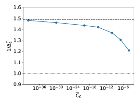
Figure 15: Estimated divergence point $\Delta_{2}^{*}$ at fixed $\Delta_{p}=0.9$ with $p=3$ as a function of the initial condition $\overline{C}$, ranging from $10^{-40}$ to $10^{-4}$. The vertical axis is in linear scale while the horizontal axis is in log-scale. We observe that the dependence of estimated divergence points on the initial condition is consistent with the asymptotic value $1/\Delta_{2}^{*}=\sqrt{2/\Delta_{p}}\approx 1.491$ following from eq. (15), and depicted by the dashed line. The dotted line instead represents the AMP threshold for comparison.

The LSE equations show a rather strong dependence on the initial condition $\overline{C}_{0}$. A low initial magnetization will give a low initial momentum in the direction of the signal, as it the can be observed in the linear expansion of $\overline{C}$ Eq. (93), and consequently the system will not be able to cross even very small barriers. The direct consequence is that reducing the initial magnetization the estimated threshold will get worse, in the sense that a larger signal-to-noise ratio will be required to find the solution. This finding can be observe in Fig. 15, where different initial conditions are compared on the section $\Delta_{p}=0.9$.

Finally we remark how the different initial conditions affect the phase diagram. In Fig. 16 we compare the Langevin hard-easy threshold evaluated starting from different initial condition, showing that the region gets larger as the initial condition decrease up to convergence.

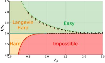
Figure 16: Phase diagram of the $p=3$ model where we compare the threshold of the Langevin hard region using different values of the initial conditions, respectively: green circles $\overline{C}_{0}=10^{-40}$, yellow circles $\overline{C}_{0}=10^{-30}$, red circles $\overline{C}_{0}=10^{-20}$.

D.6 Annealing protocol

In this section we show that using specific protocols that separate the matrix and tensor part of the cost function (something we do not allow in the main part of this paper for the purpose of having a model as generic as possible) we are able to enter in the Langevin hard region. A generic annealing scheme would lower the noises of both the channels simultaneously, which will not be able to avoid the Langevin hard region. Instead we can use the following protocol

$$\begin{split}&T_{2}\equiv 1\,,\\ &T_{p}\equiv T_{p}(t)=1+\frac{C}{\Delta_{p}}e^{-\frac{t}{\tau_{\text{ann}}}}\ .\end{split}$$ (112)

The constant $C$ allows to select at the initial time the desired effective $\Delta_{p,{\rm eff}}=\Delta_{p}+Ce^{-\frac{t}{\tau_{\text{ann}}}}$ far from (and much larger than) the original one. Instead $\tau_{\text{ann}}$ chooses the speed of the annealing protocol. Fig. 18 shows that using this protocol we are able to enter in Langevin Hard region even with $\Delta_{2}$ close to the AMP threshold. To this purpose we initiated the effective $\Delta_{p,{\rm eff}}$ close to $100$ (i.e. $C=100$), very far from the Langevin hard region, and we used different speeds for the annealing of $\Delta_{p}$ (different colors in the figures). In the figures we can observe that approaching the $\Delta_{2}=1$ we need slower and slower protocols (larger and larger $\tau_{\text{ann}}$). The reason for this behavior is due to the fact that approaching $\Delta_{2}=1$ with $\Delta_{p}=100$ a longer time is required to gain a non trivial overlap with the solution. Evidence of this growing timescale at $\Delta_{p}=100$ is given in Fig. 19 where we show the relaxation time for magnetizing to the solution varying $\Delta_{2}$. In particular, we can observe that at $\Delta_{2}=0.70$ the relaxation time is of the order of $100$ time units.

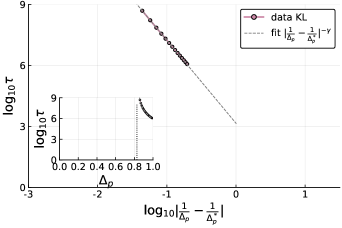
(a) $\Delta_{2}=1.01$: estimation $0.82857$ (AMP $0.82719$)

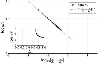
(b) $\Delta_{2}=1.05$: estimation $0.67447$ (AMP $0.67382$)

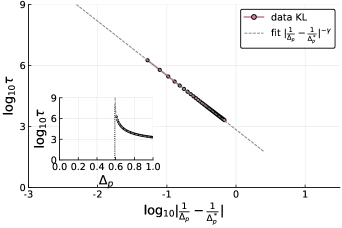
(c) $\Delta_{2}=1.10$: estimation $0.59104$ (AMP $0.59034$)

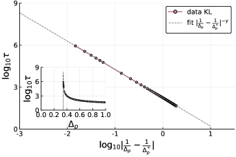
(d) $\Delta_{2}=2.00$: estimation $0.34326$ (AMP $0.34314$)

Figure 17: Relaxation time obtained from the LSE starting from an informative initial condition $\overline{C}_{0}=1$. The four cases refers to the $2+3$ model and are fitted with a power law and the relaxation time appears to diverge very close to point predicted by AMP (the AMP prediction is given in the captions).

For the protocol to be successful it is therefore crucial that the annealing time $\tau_{ann}$ is large enough to give the possibility of magnetizing the solution before $\Delta_{p,{\rm eff}}$ has significantly decreased towards $\Delta_{p}$. According to this analysis, it is not surprising that in Fig. 18 for $\Delta_{2}=0.90$ the proposed protocol seems not to be successful. For this value of the parameter $\Delta_{2}$, the time to find a solution even with $\Delta_{p}=100$ should be larger than $1000$ time units, which is much larger than the used $\tau_{ann}$ and anyway out of the time window of our numerical solution. However, with an annealing time large enough it would be in principle possible to recover exactly the same boundaries of the AMP easy region.

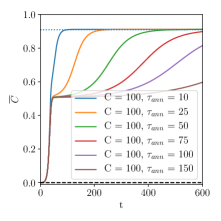
(a) $\Delta_{2}=0.50$, $\Delta_{p}=0.10$

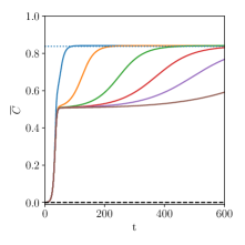
(b) $\Delta_{2}=0.50$, $\Delta_{p}=0.20$

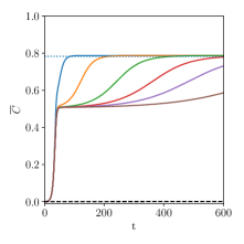
(c) $\Delta_{2}=0.50$, $\Delta_{p}=0.30$

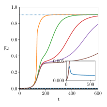
(d) $\Delta_{2}=0.70$, $\Delta_{p}=0.10$

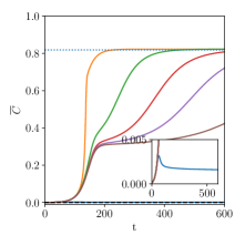
(e) $\Delta_{2}=0.70$, $\Delta_{p}=0.20$

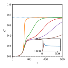
(f) $\Delta_{2}=0.70$, $\Delta_{p}=0.30$

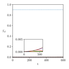
(g) $\Delta_{2}=0.90$, $\Delta_{p}=0.10$

(h) $\Delta_{2}=0.90$, $\Delta_{p}=0.20$

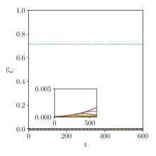
(i) $\Delta_{2}=0.90$, $\Delta_{p}=0.30$

Figure 18: The figures show the correlation with the signal in time obtained using different annealing protocols, whose details are reported in the legend of the first figure. All the protocols have $C=100$ which means that all the dynamics start with close effective $\Delta_{p}\sim 100$, $T_{p}(0)\Delta_{p}\simeq 100$ and start with an initial overlap $\overline{C}_{0}=10^{-4}$. What changes among the different lines is the relaxation speed, from the fastest, drawn in blue, to the slowest, drown in brown. They are compared with the asymptotic value of AMP, dotted line, and the Langevin dynamics without tensor-annealing, dashed line.

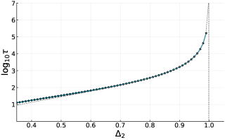
Figure 19: Relaxation times of Langevin dynamics at $\Delta_{p}=100$ without using protocols starting from $\overline{C}_{0}=10^{-4}$.

Appendix E Glassy nature of the Langevin hard phase: the replica approach

In this section we study the landscape of the spiked matrix-tensor problem following the approach of Antenucci et al. (2019). We underline here that we are interested in studying the free energy landscape problem rather than the energy landscape since the former is the relevant quantity for finite temperatures ($\beta=1$ in our case, as discussed in Sec. A). The results of Antenucci et al. (2019) suggest that the AMP-hard phase and part of the AMP-easy phase are glassy. Therefore we could expect that low magnetization glassy states trap the Langevin algorithm and forbid the relaxation to the equilibrium configurations that surrounds the signal. This may happen also in a region where AMP instead is perfectly fine in producing configurations strongly correlated with the signal. In order to check this hypothesis we compute the logarithm of the number of glassy states, called the complexity by using the replica method Monasson (1995); Antenucci et al. (2019). The goal of this analysis is to trace an additional line in the phase diagram that delimits the region where stable one step replica symmetry breaking (1RSB) metastable states exist. We conjecture that this provides a physical lower bound to the Langevin hard phase in the $(\Delta_{p},1/\Delta_{2})$ phase diagram.

E.1 Computation of the complexity through the replica method

The replica trick is based on the simple identity: $\mathbb{E}\log x=\lim_{n\rightarrow 0}\frac{\partial}{\partial n}\mathbb{E}x^{n}$. Using this observation we can compute the expected value of the free energy, $\Phi=-(\log Z)/N$, averaging the $Z^{n}$ and taking the limit $n\rightarrow 0$. This is in general as difficult as the initial problem, however, if we consider only integer $n$ and extrapolate to $0$, the computation becomes much less involved due to the fact that for integer $n$ the average $\mathbb{E}x^{n}$ can be sometimes performed analytically. Indeed in this case the replicated partition function $Z^{n}$ can be regarded as the partition function of $n$ identical uncoupled systems or replicas. Averaging over the disorder we obtain a clean system of interacting replicas. The Hamiltonian of this system displays an emerging replica symmetry since it is left unchanged by a permutation of replicas. This symmetry can be spontaneously broken in certain disordered models where frustration is sufficiently strong Mézard et al. (1987).

In mean field models characterized by fully connected factor graphs, the resulting Hamiltonian of interacting replicas depends on the configuration of the system only through a simple order parameter, the overlap $\tilde{Q}$ between them, which is a $n\times n$ matrix that describes the similarities of the configurations of different replicas in phase space. Furthermore the Hamiltonian is proportional to $N$ which means that in the thermodynamic limit $N\to\infty$, the model can be solved using the saddle point method. In this case one needs to consider a simple ansatz for the saddle point structure of the matrix $\tilde{Q}$ that allows to take the analytic continuation for $n\to 0$. The solution to this problem comes from spin glass theory and general details can be found in Mézard et al. (1987). The saddle point solutions for $\tilde{Q}$ can be classified according to the replica symmetry breaking level going from the replica symmetric solution where replica symmetry is not spontaneously broken to various degree of spontaneous replica symmetry breaking (including full-replica symmetry breaking). Here we will not review this subject but the interested reader can find details in Mézard et al. (1987). The model we are analyzing can be studied in full generality at any degree of RSB (see for example Crisanti and Leuzzi (2004, 2006, 2013) where the same models have been studied in absence of a signal). However here we will limit ourselves to consider saddle point solutions up to a 1RSB level.

The complexity of the landscape can be directly related to replica symmetry breaking. A replica symmetric solution implies an ergodic free energy landscape characterized by a single pure state. When replica symmetry is broken instead, a large number of pure states arises and the phase space gets clustered in a hierarchical way Mézard et al. (1987). Making a 1RSB approximation means to look for a situation in which the hierarchical organization contains just one level: the phase space gets clustered into an exponential number of pure states with no further internal structure.

If we assume a 1RSB glassy landscape, we can compute the complexity of metastable states using a recipe due to Monasson Monasson (1995) (see also Zamponi (2010) for a pedagogical introduction). The argument goes as follows.

Let us consider system with $x$ real replicas infinitesimally coupled. If the free energy landscape is clustered into an exponential number of metastable states, the replicated partition function, namely the partition function of the system of $x$ real replicas, can be written as

$$Z^{x}\simeq e^{N[\Sigma(f^{*})-x\beta f^{*}]}$$

where $f^{*}$ is the internal free energy of the dominant metastable states that is determined by the saddle point condition $\frac{d\Sigma}{df}(f^{*})=\beta x$ and $\beta$ the inverse temperature. Note that since we are interested in the Bayes optimal case, this corresponds to set $\beta=1$. In the analysis we will consider a generic $\beta$ before taking the limits in order to derive the averaged energy by taking its derivative. The function $\Sigma(f)$ is the complexity of metastable states having internal entropy $f$. Therefore, using the free parameter $x$ we can reconstruct the form of $\Sigma(f)$ from the replicated free energy. In order to compute the replicated free energy we need to apply the replica trick on the replicated system, $\overline{\log Z^{x}}=\lim_{n\rightarrow 0}\frac{\partial}{\partial n}\overline{(Z^{x})^{n}}$. Calling the replicated free energy $\Phi=-\frac{1}{N}\overline{\log Z^{x}}$, we get the complexity as $\Sigma=x\frac{\partial\Phi}{\partial x}-\Phi$.

We can now specify the computation to our case where the partition function is the normalization of the posterior measure. With simple manipulations of the equations Castellani and Cavagna (2005), the partition function can be expressed as the integral over the overlap matrix

$$\overline{(Z^{x})^{n}}=\overline{Z_{x}^{n}}\propto\int\prod_{ab}dQ_{ab}e^{\beta NnxS(Q)}\simeq\limsup_{Q}e^{\beta NnxS(Q)}\,;$$ (113)

where the overlap $Q$ is a $(nx+1)\times(nx+1)$ matrix

$$Q=\left(\begin{array}[]{c|c}1&m\cdots m\\ \hline\cr m&\raisebox{-15.0pt}{{\huge\mbox{$\tilde{Q}$}}}\\[-17.22217pt] \vdots&\\[-2.15277pt] m&\end{array}\right)$$

that contains a special row and column that encodes the overlap between different replicas with the signal and therefore the corresponding overlap is the magnetization $m$.

The 1RSB structure for the matrix $\tilde{Q}$ can be obtained by defining the following $nx\times nx$ matrices: the identity matrix $\mathbb{I}_{ij}=\delta_{ij}$, the full matrix $\mathbb{J}^{(0)}_{nx,ij}=1$, and $\mathbb{J}_{nx}^{(1)}=\text{diag}(J_{x}^{(0)},\dots,J_{x}^{(0)})$ a block diagonal matrix where the diagonal blocks $J_{x}^{(0)}$ have size $x\times x$ and are matrices full of 1. In this case the 1RSB ansatz for $\tilde{Q}$ reads

$$\tilde{Q}=(1-q_{M})\mathbb{I}_{nx}+(q_{M}-q_{m})\mathbb{J}_{nx}^{(1)}+q_{m}\mathbb{J}_{nx}^{(0)}\,.$$

Using this ansatz we can compute $S(Q)$ that is given by

$$\begin{split}\beta S(Q)&=\frac{1}{nx}\left[\frac{1}{2}\log\text{det}\;Q+\frac{\beta^{2}}{2p\Delta_{p}}\sum_{a,b=1}^{n}Q_{ab}^{p}+\frac{\beta^{2}}{4\Delta_{2}}\sum_{a,b=1}^{n}Q_{ab}^{2}+\frac{\beta}{p\Delta_{p}}\sum_{a=1}^{n}Q_{0a}^{p}+\frac{\beta}{2\Delta_{2}}\sum_{a=1}^{n}Q_{0a}^{2}\right]=\\ &=\frac{1}{2}\log(1-q_{M})+\frac{1}{2x}\log\frac{1-q_{M}+x(q_{M}-q_{m})}{1-q_{M}}+\frac{1}{2}\frac{q_{m}-m^{2}}{1-q_{M}+x(q_{M}-q_{m})}+\\ &+\frac{\beta^{2}}{2p\Delta_{p}}\left(1-q_{M}^{p}+x(q_{M}^{p}-q_{m}^{p})+\frac{2}{\beta}m^{p}\right)+\frac{\beta^{2}}{4\Delta_{2}}\left(1-q_{M}^{2}+x(q_{M}^{2}-q_{m}^{2})+\frac{2}{\beta}m^{2}\right)\,.\end{split}$$ (114)

From Eq. (114) we obtain the saddle point equations

$$\begin{split}&0=2\frac{\partial S}{\partial q_{M}}=(x-1)\left[\frac{1}{x}\left(\frac{1}{1-q_{M}+x(q_{M}-q_{m})}-\frac{1}{1-q_{M}}\right)-\frac{q_{m}-m^{2}}{[1-q_{M}+x(q_{M}-q_{m})]^{2}}+\beta^{2}\left(\frac{q_{M}^{p-1}}{\Delta_{p}}+\frac{q_{M}}{\Delta_{2}}\right)\right]\,;\\ &0=2\frac{\partial S}{\partial q_{m}}=x\left[\frac{q_{m}-m^{2}}{[1-q_{M}+x(q_{M}-q_{m})]^{2}}-\beta^{2}\left(\frac{q_{m}^{p-1}}{\Delta_{p}}+\frac{q_{m}}{\Delta_{2}}\right)\right]\,;\\ &0=\frac{\partial S}{\partial m}=\frac{-m}{1-q_{M}+x(q_{M}-q_{m})}+\beta^{2}\left(\frac{m^{p-1}}{\Delta_{p}}+\frac{m}{\Delta_{2}}\right)\,.\end{split}$$ (115)

The above 1RSB fixed point equations can be used to derive the de Almeida-Thouless instability of the RS solution towards 1RSB. This stability condition, sometimes called the replicon also determines the overlap of the marginal threshold states. The stability analysis is done by expansion of eqs. (115) in a small parameters $q_{M}-q_{m}=\varepsilon\ll 1$ and investigating whether under iterations such a small difference grows of decreases. This leads directly to the threshold condition on the overlap

$$\frac{1}{\beta^{2}(1-q^{\rm th})^{2}}=(p-1)\frac{(q^{\rm th})^{(p-2)}}{\Delta_{p}}+\frac{1}{\Delta_{2}}\,.$$ (116)

This condition is then used in the derivation of the Langevin threshold (15) in the main text.

From Eq. (114) we obtain also the averaged energy

$$E=\frac{\partial\overline{\log Z^{x}}}{\partial\beta}\Big{|}_{\beta=1}=\frac{1-q_{M}^{p}+x(q_{M}^{p}-q_{m}^{p})+m^{p}}{p\Delta_{p}}+\frac{1-q_{M}^{2}+x(q_{M}^{2}-q_{m}^{2})+m^{2}}{2\Delta_{2}}\,.$$ (117)

In particular the threshold states are characterized by $q_{M}=q^{\text{\rm th}}$, fixed by Eq. (116), $q_{m}=0$ and $m=0$. Imposing these values, we can use the saddle point equation for $q_{M}$, Eq. 115, to fix the Parisi parameters $x$,

$$x(q^{\text{\rm th}})=\frac{1}{(1-q^{\text{\rm th}})\left[\frac{(q^{\text{\rm th}})^{p-1}}{\Delta_{p}}+\frac{q^{\text{\rm th}}}{\Delta_{2}}\right]}-\frac{1}{q^{\text{\rm th}}}+1\;.$$ (118)

These pieces together give Eq. (12) showed in the main text.

Having obtained the energy we can consider $\beta=1$ fixed for the rest of the analysis. We can observe that starting from this expression we can derive the RS free energy, (41), $q_{M}=q_{m}$ or equivalently in the limit $x\rightarrow 1$. The low magnetization solution to these equations gives the complexity of the metastable branch of the posterior measure which is given by

$$\begin{split}-\Sigma(x;Q^{*})&=-\frac{1}{2}\log\frac{1-q_{M}+x(q_{M}-q_{m})}{1-q_{M}}+\frac{x}{2}\frac{q_{M}-q_{m}}{1-q_{M}+x(q_{M}-q_{m})}-\frac{x^{2}}{2}\frac{(q_{m}-m^{2})(q_{M}-q_{m})}{[1-q_{M}+x(q_{M}-q_{m})]^{2}}+\frac{x^{2}}{2}\frac{q_{M}^{p}-q_{m}^{p}}{p\Delta_{p}}+\\ &+\frac{x^{2}}{2}\frac{q_{M}^{2}-q_{m}^{2}}{2\Delta_{2}}\,.\end{split}$$ (119)

The free parameter $x$ allows us to tune the free energy of the states of which we compute the complexity. Thus we can characterize the part of the phase diagram where an exponential number of states is present.

To complete the 1RSB analysis we compute the stability of the 1RSB saddle point solution for $Q$. This is done analogously to the derivation of the replicon condition (116), analyzing stability of the 1RSB towards further replica symmetry breaking. Following Crisanti and Sommers (1992); Crisanti and Leuzzi (2013) we obtain two replicon eigenvalues given by

$$\lambda_{I} =1-(1-q_{M}+x(q_{M}-q_{m}))^{2}\left[(p-1)\frac{q_{m}^{p-2}}{\Delta_{p}}+\frac{1}{\Delta_{2}}\right]\,,$$ (120)

$$\lambda_{II} =1-(1-q_{M})^{2}\left[(p-1)\frac{q_{M}^{p-2}}{\Delta_{p}}+\frac{1}{\Delta_{2}}\right]\,.$$ (121)

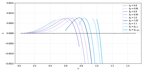
Figure 20: Complexity with as a function of the Parisi parameter $x$ for $p=3$ on the line $\Delta_{p}=0.5$. The solid line characterizes the stable part of the complexity while the dashed line the unstable one.

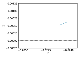
(a) $p=3$; $\Delta_{p}=0.50$; $\Delta_{2}=0.85$

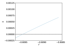
(b) $p=3$; $\Delta_{p}=0.50$; $\Delta_{2}=0.90$

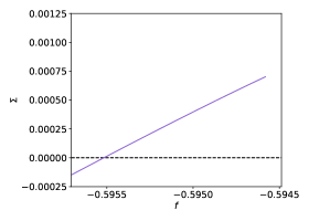
(c) $p=3$; $\Delta_{p}=0.50$; $\Delta_{2}=0.95$

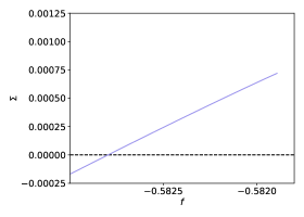
(d) $p=3$; $\Delta_{p}=0.50$; $\Delta_{2}=1.00$

Figure 21: The stable part of the 1RSB complexity as a function of the free energy for $p=3$ and $\Delta_{p}=0.5$.

We can analyze what happens to the landscape when we fix $\Delta_{p}<1$ and we start from a large value of $\Delta_{2}<\Delta_{2,{\rm dyn}}(\Delta_{p})$ and we decrease $\Delta_{2}$. In this case for sufficiently high $\Delta_{2}$ and large enough $\Delta_{p}$ the system is in a paramagnetic phase and no glassy states are present. At the dynamical transition line instead we find a positive complexity as plotted in Fig. 20. At this point the equilibrium states that dominate the posterior measure are the so called threshold states for which the complexity is maximal. For those states the eigenvalue $\lambda_{II}=0$ which confirms that these states are marginally stable Cugliandolo and Kurchan (1993). Decreasing $\Delta_{2}$ one crosses the information theoretic phase transition where the relevant metastable states that dominate the posterior measure have zero complexity. This corresponds to a freezing/condensation/Kauzmann transition. Below the information theoretic phase transition the thermodynamics of the posterior measure is dominated by the state containing the signal. However one can neglect the high magnetization solution of the 1RSB equations to get the properties of the metastable branch and computing the complexity of states that have zero overlap with the signal. The complexity curves as a function of the Parisi parameter $x$ for decreasing values of $\Delta_{2}$ are plotted in Fig. 20 for fixed $\Delta_{p}=0.5$ and several $\Delta_{2}$. The curves contain a stable 1RSB part and an unstable one where $\lambda_{II}$ is negative. The 1RSB line shown in Figs. 14 is obtained by looking at when the states with positive complexity and $\lambda_{II}=0$ disappear. This means that it gives the point where the 1RSB marginally stable states disappear and therefore it is expected to be a lower bound for the disappearance of glassiness in the phase diagram. The important outcome of this analysis is that for $\Delta_{2}<1$ but not sufficiently small, namely in part of the AMP-easy phase, the replica analysis predicts the existence of 1RSB marginally stable glassy states that may trap the Langevin algorithm from relaxing towards the signal Antenucci et al. (2019) and therefore supports the existence of the Langevin hard phase. This approach, however, does not predict quantitatively correctly the extent on the Langevin-hard phase for reasons that remain obscure and should be investigated further.

Finally in Fig. 21 we plot the complexity as a function of the internal free energy of the metastable states for some values of $\Delta_{2}$ and $\Delta_{p}$.

E.2 Breakdown of the fluctuation-dissipation theorem in the Langevin hard phase

When the Langevin algorithm is able to reach equilibrium, being it the signal or the paramagnetic state, it should satisfy the Fluctuation-Dissipation Theorem (FDT) according to which the response function is related to the correlation function through $R(t,t^{\prime})=-\frac{\partial C(t,t^{\prime})}{\partial t}$. Furthermore, time translational invariance (TTI) should arise implying that both correlation and response functions should be functions of only the time difference meaning that $R(t,t^{\prime})=R(t-t^{\prime})$ and $C(t,t^{\prime})=C(t-t^{\prime})$, note that all one time quantities are constant in equilibrium. When the dynamics is run in the glass phase, metastable states may forbid equilibration. In this case time translational invariance is never reached at long times, it is supposed to be reached only on exponential timescales in the system size, and the dynamics displays aging violating at the same time the FDT relation. The analysis of the asymptotic aging dynamics has been cracked by Cugliandolo and Kurchan in Cugliandolo and Kurchan (1993, 1995) (see also Cugliandolo (2003) for a pedagogical review) in the simplest spin glass model (see also Cugliandolo and Kurchan (1994) for a much more complex situation) where no signal is present. The outcome of this work is that when the dynamics started from a random initial conditions is run in the glass phase, it drives the system to surf on the threshold states. In the model analyzed in Cugliandolo and Kurchan (1993) these states correspond to the 1RSB marginally stable glassy states that maximize the complexity. In this section we analyze the Cugliandolo-Kurchan scenario by contrasting the numerical solution of the dynamical equations with the replica analysis of the complexity. According to Cugliandolo and Kurchan (1993), the long time Langevin dynamics, but still for times that are not exponentially large in the system size $N$, can be characterized by two time regimes. For short times differences $t-t^{\prime}\sim{\cal O}(1)$ and $t^{\prime}\to\infty$, the system obeys the FDT theorem and TTI; this regime can be understood as a first fast local equilibration in the nearest metastable state available. On a longer timescale $t-t^{\prime}\to\infty$ and $t/t^{\prime}<\infty$, the dynamics surfs on threshold states and FDT and TTI are both violated. In this time window, both the response and correlation functions become functions of $\lambda=h(t)/h(t^{\prime})$ being $h(t)$ an arbitrary reparametrization of the time variable. The function $h(t)$ must be a monotonously increasing function. The asymptotic reparametrization invariance is a key property of the dynamical equations Cugliandolo and Kurchan (1993). By defining ${\cal C(\lambda)}=C(t,t^{\prime})$ and ${\cal R(\lambda)}=tR(t,t^{\prime})$ the Cugliandolo-Kurchan solution implies that in this aging regime the FDT relation can be generalized to

$$\mathcal{R}\left(\lambda\right)=x\ \mathcal{C}^{\prime}\left(\lambda\right)$$ (122)

with $x$ an effective FDT ratio that controls how much the FDT is violated. In the scenario of Cugliandolo and Kurchan (1993), the value of $x$ coincides with the 1RSB Parisi parameter that corresponds to threshold states computed within the replica approach. In order to test this picture we follow Cugliandolo and Kurchan Cugliandolo and Kurchan (1997) and we plot the integrated response ${\cal{F}}(t,t^{\prime})=-\int_{t^{\prime}}^{t}R(t,t^{\prime\prime})dt^{\prime\prime}$ as a function of $C(t,t^{\prime})$ in a parametric way. This is done in Fig. 22.

If FDT holds at all timescales, one should see a straight line with slope $-1$. Instead what we see in the Langevin hard phase is that for large values of $t^{\prime}$ the curves approach asymptotically for $t^{\prime}\gg 1$ two straight lines. For high values of $\cal C$, meaning for short time differences $t-t^{\prime}\sim{\cal O}(1)$, the slope of the straight line is $-1$ which means that ${\cal F}=1-{\cal C}$ as implied by the short time FDT relation. On longer timescales FDT is violated, confirming the glassiness of the Langevin hard phase. By doing a linear fit we can use the data plotted in Fig. 22 to estimate the FDT ratio $x$ appearing in Eq. (122). This can be compared with the Parisi parameter $x$ for which we have marginally stable 1RSB states. We find an overall very good agreement (data coming from the fit is reported in the caption of Fig. 22). The small discrepancy between the two values of $x$ can be either due to the numerical accuracy in solving the dynamical equations as well as the possibility that the 1RSB threshold is not exactly the one that characterizes the long time dynamics. Further investigations are needed to clarify this point. Finally, according to Cugliandolo and Kurchan (1993) the value of $\cal C$ at which the two straight line cross should coincide with the value of $q_{M}$ computed for the threshold states within the 1RSB solution. Again we find a very good agreement.

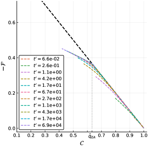
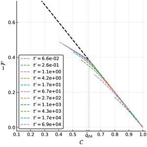
Figure 22: Left panel: parametric plot of integrate response function with respect to correlation function for $p=3$, $\Delta_{2}=0.8$ and $\Delta_{p}=0.2$. The different lines represent different waiting time, $t^{\prime}$. The black dashed line correspond to the FDT prediction $x=1$. The vertical dotted line is the point where we observe a kink, which we denote by ${\cal C}=\hat{q}_{EA}$ and should be equal to the saddle point value of $q_{M}$ as extracted from the 1RSB threshold states in the replica computation Cugliandolo and Kurchan (1993): $\hat{q}_{EA}=0.633$ and $q_{M}=0.638$. For $\mathcal{C}$ smaller than $q_{EA}$ the FDT is violated and is replaced by a generalized version as in Eq. (122). We can obtain the value of the FDT ratio from a fit of the slope of the asymptotic curves for ${\cal C}<\hat{q}_{EA}$. We obtain $\hat{x}=0.397$ which should be compared with the Parisi parameter that corresponds to 1RSB marginally stable states obtained from the replica computation that is $x=0.408$. Right panel: parametric plot of the integrated response as a function of the correlation for $p=3$ and $\Delta_{2}=1.4$ and $\Delta_{p}=0.2$. In this case the value of the FDT ratio extracted from fitting the data is $\hat{x}=0.397$ to be compared with the value of the Parisi parameter for the 1RSB threshold states that is $x=0.408$. At the same time data gives $\hat{q}_{EA}=0.633$ while the replica computation gives $q_{M}=0.638$.

Appendix F Free-energy Hessian, BBP transition and Langevin threshold

In the following we present the derivation and the analysis of the Langevin threshold based on the study of the free energy Hessian. The starting point of the analysis is the so-called TAP free energy, i.e. the free energy as a function of the local magnetizations. The TAP free-energy was introduced in the early days of spin-glass theory Thouless et al. ; Mézard et al. (1987) and is now receiving a lot of attention in the mathematical community, see e.g. Chen and Panchenko (2018). A straightforward generalization of the results of Crisanti and Sommers (1995) allows one to obtain the TAP free energy for the model considered in this work, i.e. for the Hamiltonian (4):

$$F(\{m_{i}\})=-\frac{\sqrt{(p-1)!}}{\Delta_{p}N^{(p-1)/2}}\sum_{i_{1}<\dots<i_{p}}T_{i_{1}\dots i_{p}}m_{i_{1}}\dots m_{i_{p}}\\ -\frac{1}{\Delta_{2}\sqrt{N}}\sum_{i<j}Y_{ij}m_{i}m_{j}+f(q)N\,.$$

where we have set the temperature to one, $q=\sum_{i}m_{i}^{2}/N$ and $f(q)$ reads:

$$f(q)=-\frac{1}{2}\log(1-q)-\frac{1}{2p\Delta_{p}}\left[1+(p-1)q^{p}-pq^{p-1}\right]-\frac{1}{4\Delta_{2}}\left[1+q^{2}-2q\right]\,.$$

The so-called TAP states are local minima of $F(\{m_{i}\})$. We are interested in the free energy Hessian evaluated at the TAP states having zero overlap with the signal:

$$\frac{\partial^{2}F}{\partial m_{i}\partial m_{j}}=G_{ij}+\delta_{ij}f^{\prime}(q)-\frac{1}{\Delta_{2}}\frac{x_{i}^{*}x_{j}^{*}}{N}+f^{\prime\prime}(q)\frac{m_{i}m_{j}}{N}\,,$$ (123)

where the matrix $G_{ij}$ is defined as

$$G_{ij}=-\frac{1}{\Delta_{2}\sqrt{N}}\xi_{ij}-\frac{\sqrt{(p-1)!}}{\Delta_{p}N^{(p-1)/2}(p-2)!}\sum_{i_{1},\dots,i_{p-2}}\xi_{iji_{1}\dots i_{p-2}}m_{i_{1}}\dots m_{i_{p-2}}\,.$$

As shown originally in the spin-glass literature Bray and Moore (1979), and recently put on a firmer basis by the Kac-Rice method Auffinger et al. (2013); Ros et al. (2019), the matrix $G_{ij}$ is statistically equivalent to a random matrix belonging to the Gaussian Orthogonal Ensemble (GOE). In our case, the corresponding GOE matrix has elements which are i.i.d. Gaussian random variables with mean zero and variance $\sigma^{2}_{F}/N$, where

$$\sigma^{2}_{F}(q)=\frac{(p-1)q^{p-2}}{\Delta_{p}}+\frac{1}{\Delta_{2}}\,.$$

Neglecting for the moment the last two terms in eq. (14), one finds that the free-energy Hessian is the sum of a GOE matrix and the identity multiplied by $f^{\prime}(q)$. The corresponding density of eigenvalues is therefore the Wigner semicircle with support $[-2\sigma_{F}(q)+f^{\prime}(q),2\sigma_{F}(q)+f^{\prime}(q)]$. This result is valid for any TAP state. The threshold states, which are the ones trapping the Langevin dynamics, are characterized by a vanishing fraction of zero modes, i.e. the left edge of the support of the Wigner semi-circle is zero. Their overlap is therefore fixed by the equation:

$$2\sigma_{F}(q_{\rm th})=f^{\prime}(q_{\rm th})\qquad\rightarrow\qquad\frac{1}{1-q_{\rm th}}=\sqrt{\frac{(p-1)q_{\rm th}^{p-2}}{\Delta_{p}}+\frac{1}{\Delta_{2}}}\,.$$ (124)

Let’s consider now the role of the last two terms in eq. (14). Both are rank-one perturbations and hence can lead to a BBP transition Baik et al. (2005), i.e. an eigenvalue that pops out of the Wigner semi-circle with an eigenvector having a finite overlap in the direction of the perturbation. It can be easily checked that $f^{\prime\prime}(q_{\rm th})\geq 0$; therefore the last term cannot lead to any negative eigenvalue and does not play any role in determining the stability of the threshold states. It is the other term which is responsible for the instability in the direction of the signal. In fact, it is the contribution due to the spike; it becomes larger when the signal to noise ratio, $1/\Delta_{2}$, increases.

The condition for the BBP transition for a GOE matrix having elements with variance $\sigma_{F}^{2}/N$ and which is perturbed by a rank one perturbation of strength $1/\Delta_{2}$ is $\frac{1}{\Delta_{2}}=\sigma_{F}$. This is the equation for the Langevin threshold:

$$\frac{1}{\Delta_{2}}=\sqrt{\frac{(p-1)q_{\rm th}^{p-2}}{\Delta_{p}}+\frac{1}{\Delta_{2}}}\ ,$$

Together with (124), this leads to the equation (15) presented in the main text and implies $q_{\rm th}=1-\Delta_{2}^{*}$ at the Langevin threshold.

References

• Bottou (2010) L. Bottou, Large-scale machine learning with stochastic gradient descent, in Proceedings of COMPSTAT’2010 (Springer, 2010) pp. 177–186.
• Welling and Teh (2011) M. Welling and Y. W. Teh, Bayesian learning via stochastic gradient Langevin dynamics, in Proceedings of the 28th International Conference on Machine Learning (ICML-11) (2011) pp. 681–688.
• LeCun et al. (2015) Y. LeCun, Y. Bengio, and G. Hinton, Deep learning, Nature 521, 436 (2015).
• Bouchaud et al. (1998) J.-P. Bouchaud, L. F. Cugliandolo, J. Kurchan, and M. Mézard, Out of equilibrium dynamics in spin-glasses and other glassy systems, Spin glasses and random fields , 161 (1998).
• Seung et al. (1992) H. S. Seung, H. Sompolinsky, and N. Tishby, Statistical mechanics of learning from examples, Phys. Rev. A 45, 6056 (1992).
• Zdeborová and Krzakala (2016) L. Zdeborová and F. Krzakala, Statistical physics of inference: thresholds and algorithms, Advances in Physics 65, 453 (2016)http://dx.doi.org/10.1080/00018732.2016.1211393 .
• Deshpande and Montanari (2015) Y. Deshpande and A. Montanari, Finding hidden cliques of size $\sqrt{(N/e)}$ in nearly linear time, Foundations of Computational Mathematics 15, 1069 (2015).
• Barbier et al. (2019) J. Barbier, F. Krzakala, N. Macris, L. Miolane, and L. Zdeborová, Optimal errors and phase transitions in high-dimensional generalized linear models, Proceedings of the National Academy of Sciences 116, 5451 (2019).
• Barbier et al. (2016) J. Barbier, M. Dia, N. Macris, F. Krzakala, T. Lesieur, and L. Zdeborová, Mutual information for symmetric rank-one matrix estimation: A proof of the replica formula, in Advances in Neural Information Processing Systems 29 (2016) p. 424–432.
• Lesieur et al. (2017a) T. Lesieur, L. Miolane, M. Lelarge, F. Krzakala, and L. Zdeborová, Statistical and computational phase transitions in spiked tensor estimation, in Information Theory (ISIT), 2017 IEEE International Symposium on (IEEE, 2017) pp. 511–515.
• Aubin et al. (2018) B. Aubin, A. Maillard, J. Barbier, F. Krzakala, N. Macris, and L. Zdeborová, The committee machine: Computational to statistical gaps in learning a two-layers neural network, in Advances in Neural Information Processing Systems (2018).
• Donoho et al. (2009) D. L. Donoho, A. Maleki, and A. Montanari, Message-passing algorithms for compressed sensing, Proceedings of the National Academy of Sciences 106, 18914 (2009).
• Krzakala et al. (2013) F. Krzakala, C. Moore, E. Mossel, J. Neeman, A. Sly, L. Zdeborová, and P. Zhang, Spectral redemption in clustering sparse networks, Proceedings of the National Academy of Science 110, 20935 (2013)arXiv:1306.5550 .
• Hopkins and Steurer (2017) S. B. Hopkins and D. Steurer, Bayesian estimation from few samples: community detection and related problems, arXiv preprint arXiv:1710.00264  (2017).
• Baik et al. (2005) J. Baik, G. B. Arous, S. Péché, et al., Phase transition of the largest eigenvalue for nonnull complex sample covariance matrices, The Annals of Probability 33, 1643 (2005).
• Johnstone and Lu (2009) I. M. Johnstone and A. Y. Lu, On consistency and sparsity for principal components analysis in high dimensions, Journal of the American Statistical Association 104, 682 (2009).
• Anandkumar et al. (2014) A. Anandkumar, R. Ge, D. Hsu, S. M. Kakade, and M. Telgarsky, Tensor decompositions for learning latent variable models, The Journal of Machine Learning Research 15, 2773 (2014).
• Richard and Montanari (2014) E. Richard and A. Montanari, A statistical model for tensor PCA, in Advances in Neural Information Processing Systems (2014) pp. 2897–2905.
• Hopkins et al. (2015) S. B. Hopkins, J. Shi, and D. Steurer, Tensor principal component analysis via sum-of-square proofs, in Conference on Learning Theory (2015) pp. 956–1006.
• Ge and Ma (2017) R. Ge and T. Ma, On the optimization landscape of tensor decompositions, in Advances in Neural Information Processing Systems (2017) pp. 3653–3663.
• Arous et al. (2018) G. B. Arous, R. Gheissari, and A. Jagannath, Algorithmic thresholds for tensor PCA, arXiv preprint arXiv:1808.00921  (2018).
• Ros et al. (2019) V. Ros, G. B. Arous, G. Biroli, and C. Cammarota, Complex energy landscapes in spiked-tensor and simple glassy models: Ruggedness, arrangements of local minima, and phase transitions, Physical Review X 9, 011003 (2019).
• Krzakala and Zdeborová (2009) F. Krzakala and L. Zdeborová, Hiding quiet solutions in random constraint satisfaction problems, Physical review letters 102, 238701 (2009).
• Decelle et al. (2011) A. Decelle, F. Krzakala, C. Moore, and L. Zdeborová, Asymptotic analysis of the stochastic block model for modular networks and its algorithmic applications, Physical Review E 84, 066106 (2011).
• Antenucci et al. (2019) F. Antenucci, S. Franz, P. Urbani, and L. Zdeborová, Glassy nature of the hard phase in inference problems, Physical Review X 9, 011020 (2019).
• Crisanti et al. (1993) A. Crisanti, H. Horner, and H.-J. Sommers, The spherical $p$-spin interaction spin-glass model, Zeitschrift für Physik B Condensed Matter 92, 257 (1993).
• Cugliandolo and Kurchan (1993) L. F. Cugliandolo and J. Kurchan, Analytical solution of the off-equilibrium dynamics of a long-range spin-glass model, Physical Review Letters 71, 173 (1993).
• Ben Arous et al. (2006) G. Ben Arous, A. Dembo, and A. Guionnet, Cugliandolo-Kurchan equations for dynamics of spin-glasses, Probability theory and related fields 136, 619 (2006).
• Deshpande and Montanari (2014) Y. Deshpande and A. Montanari, Information-theoretically optimal sparse PCA, in Information Theory (ISIT), 2014 IEEE International Symposium on (IEEE, 2014) pp. 2197–2201.
• Gross and Mézard (1984) D. J. Gross and M. Mézard, The simplest spin glass, Nuclear Physics B 240, 431 (1984).
• Fyodorov (2004) Y. V. Fyodorov, Complexity of random energy landscapes, glass transition, and absolute value of the spectral determinant of random matrices, Physical review letters 92, 240601 (2004).
• Auffinger et al. (2013) A. Auffinger, G. B. Arous, and J. Černý, Random matrices and complexity of spin glasses, Communications on Pure and Applied Mathematics 66, 165 (2013).
• Sagun et al. (2014) L. Sagun, V. U. Guney, G. B. Arous, and Y. LeCun, Explorations on high dimensional landscapes, arXiv preprint arXiv:1412.6615  (2014).
• Arous et al. (2019) G. B. Arous, S. Mei, A. Montanari, and M. Nica, The landscape of the spiked tensor model, Communications on Pure and Applied Mathematics 72, 2282 (2019).
• Anandkumar et al. (2016) A. Anandkumar, Y. Deng, R. Ge, and H. Mobahi, Homotopy analysis for tensor pca, COLT 2017, arXiv:1610.09322  (2016).
• Wein et al. (2019) A. S. Wein, A. E. Alaoui, and C. Moore, The Kikuchi hierarchy and tensor PCA, arXiv preprint arXiv:1904.03858  (2019).
• Lesieur et al. (2017b) T. Lesieur, F. Krzakala, and L. Zdeborová, Constrained low-rank matrix estimation: Phase transitions, approximate message passing and applications, Journal of Statistical Mechanics: Theory and Experiment 2017, 073403 (2017b).
• Lelarge and Miolane (2016) M. Lelarge and L. Miolane, Fundamental limits of symmetric low-rank matrix estimation, Probability Theory and Related Fields , 1 (2016).
• Thouless et al. (1977) D. J. Thouless, P. W. Anderson, and R. G. Palmer, Solution of‘solvable model of a spin glass’, Philosophical Magazine 35, 593–601 (1977).
• Javanmard and Montanari (2013) A. Javanmard and A. Montanari, State evolution for general approximate message passing algorithms, with applications to spatial coupling, Information and Inference: A Journal of the IMA 2, 115 (2013).
• Crisanti and Leuzzi (2004) A. Crisanti and L. Leuzzi, Spherical 2+ p spin-glass model: An exactly solvable model for glass to spin-glass transition, Physical review letters 93, 217203 (2004).
• Crisanti and Leuzzi (2006) A. Crisanti and L. Leuzzi, Spherical 2+ p spin-glass model: An analytically solvable model with a glass-to-glass transition, Physical Review B 73, 014412 (2006).
• Martin et al. (1973) P. C. Martin, E. Siggia, and H. Rose, Statistical dynamics of classical systems, Physical Review A 8, 423 (1973).
• Mézard et al. (1987) M. Mézard, G. Parisi, and M.-A. Virasoro, Spin glass theory and beyond. (World Scientific Publishing, 1987).
• Kim and Latz (2001) B. Kim and A. Latz, The dynamics of the spherical p-spin model: From microscopic to asymptotic, EPL (Europhysics Letters) 53, 660 (2001).
• Berthier et al. (2007a) L. Berthier, G. Biroli, J.-P. Bouchaud, W. Kob, K. Miyazaki, and D. Reichman, Spontaneous and induced dynamic fluctuations in glass formers. I. General results and dependence on ensemble and dynamics, The Journal of chemical physics 126, 184503 (2007a).
• Sarao Mannelli et al. (2018) S. Sarao Mannelli, G. Biroli, C. Cammarota, F. Krzakala, P. Urbani, and L. Zdeborová, Langevin state evolution integrators (2018), available at: https://github.com/sphinxteam/spiked_matrix-tensor.
• Cugliandolo and Kurchan (1995) L. Cugliandolo and J. Kurchan, Weak ergodicity breaking in mean-field spin-glass models, Philosophical Magazine B 71, 501 (1995).
• (49) D. Thouless, P. Anderson, and R. Palmer, Solution of a solvable model of a spin glass, 1977, Phil. Mag 35, 593.
• Chen and Panchenko (2018) W.-K. Chen and D. Panchenko, On the tap free energy in the mixed p-spin models, Communications in Mathematical Physics 362, 219 (2018).
• Edwards and Jones (1976) S. F. Edwards and R. C. Jones, The eigenvalue spectrum of a large symmetric random matrix, Journal of Physics A: Mathematical and General 9, 1595 (1976).
• Crisanti and Leuzzi (2013) A. Crisanti and L. Leuzzi, Exactly solvable spin–glass models with ferromagnetic couplings: The spherical multi-p-spin model in a self-induced field, Nuclear Physics B 870, 176 (2013).
• Mézard and Montanari (2009) M. Mézard and A. Montanari, Information, physics, and computation (Oxford University Press, 2009).
• Boucheron et al. (2004) S. Boucheron, G. Lugosi, and O. Bousquet, Concentration inequalities, in Advanced Lectures on Machine Learning (Springer, 2004) pp. 208–240.
• Korada and Macris (2009) S. B. Korada and N. Macris, Exact solution of the gauge symmetric p-spin glass model on a complete graph, Journal of Statistical Physics 136, 205 (2009).
• Krzakala et al. (2016) F. Krzakala, J. Xu, and L. Zdeborová, Mutual information in rank-one matrix estimation, in 2016 IEEE Information Theory Workshop (ITW) (2016) pp. 71–75.
• Aizenman et al. (2003) M. Aizenman, R. Sims, and S. L. Starr, Extended variational principle for the sherrington-kirkpatrick spin-glass model, Physical Review B 68, 214403 (2003).
• Barbier and Macris (2018) J. Barbier and N. Macris, The adaptive interpolation method: a simple scheme to prove replica formulas in bayesian inference, Probability Theory and Related Fields , 1 (2018).
• Alaoui and Krzakala (2018) A. E. Alaoui and F. Krzakala, Estimation in the spiked wigner model: A short proof of the replica formula, in 2018 IEEE International Symposium on Information Theory (ISIT) (2018) pp. 1874–1878.
• Mourrat (2018) J.-C. Mourrat, Hamilton-Jacobi equations for mean-field disordered systems, arXiv preprint arXiv:1811.01432  (2018).
• Guo et al. (2005) D. Guo, S. Shamai, and S. Verdú, Mutual information and minimum mean-square error in gaussian channels, IEEE Transactions on Information Theory 51, 1261 (2005).
• Georgii (2011) H.-O. Georgii, Gibbs measures and phase transitions, Vol. 9 (Walter de Gruyter, 2011).
• Macris (2007) N. Macris, Griffith-Kelly-Sherman correlation inequalities: A useful tool in the theory of error correcting codes, IEEE Transactions on Information Theory 53, 664 (2007).
• Montanari (2008) A. Montanari, Estimating random variables from random sparse observations, European Transactions on Telecommunications 19, 385 (2008).
• Coja-Oghlan et al. (2017) A. Coja-Oghlan, F. Krzakala, W. Perkins, and L. Zdeborova, Information-theoretic thresholds from the cavity method, in Proceedings of the 49th Annual ACM SIGACT Symposium on Theory of Computing (STOC) (2017) pp. 146–157.
• Nishimori (2001) H. Nishimori, Statistical physics of spin glasses and information processing: an introduction, Vol. 111 (Clarendon Press, 2001).
• Guerra and Toninelli (2002) F. Guerra and F. L. Toninelli, The thermodynamic limit in mean field spin glass models, Communications in Mathematical Physics 230, 71 (2002).
• Ricci-Tersenghi et al. (2019) F. Ricci-Tersenghi, G. Semerjian, and L. Zdeborová, Typology of phase transitions in bayesian inference problems, Physical Review E 99, 042109 (2019).
• Cugliandolo (2003) L. F. Cugliandolo, Course 7: Dynamics of glassy systems, in Slow Relaxations and nonequilibrium dynamics in condensed matter (Springer, 2003) pp. 367–521.
• Castellani and Cavagna (2005) T. Castellani and A. Cavagna, Spin glass theory for pedestrians, Journal of Statistical Mechanics: Theory and Experiment 2005, P05012 (2005).
• Agoritsas et al. (2018) E. Agoritsas, G. Biroli, P. Urbani, and F. Zamponi, Out-of-equilibrium dynamical mean-field equations for the perceptron model, Journal of Physics A: Mathematical and Theoretical 51, 085002 (2018).
• Berthier et al. (2007b) L. Berthier, G. Biroli, J.-P. Bouchaud, W. Kob, K. Miyazaki, and D. R. Reichman, Spontaneous and induced dynamic correlations in glass formers. II. Model calculations and comparison to numerical simulations, The Journal of chemical physics 126, 184504 (2007b).
• Monasson (1995) R. Monasson, Structural glass transition and the entropy of the metastable states, Physical review letters 75, 2847 (1995).
• Zamponi (2010) F. Zamponi, Mean field theory of spin glasses, arXiv preprint arXiv:1008.4844  (2010).
• Crisanti and Sommers (1992) A. Crisanti and H.-J. Sommers, The spherical p-spin interaction spin glass model: the statics, Zeitschrift für Physik B Condensed Matter 87, 341 (1992).
• Cugliandolo and Kurchan (1994) L. Cugliandolo and J. Kurchan, On the out-of-equilibrium relaxation of the Sherrington-Kirkpatrick model, Journal of Physics A: Mathematical and General 27, 5749 (1994).
• Cugliandolo and Kurchan (1997) L. F. Cugliandolo and J. Kurchan, Aging and effective temperatures in the low temperature mode-coupling equations, Progress of Theoretical Physics Supplement 126, 407 (1997).
• Crisanti and Sommers (1995) A. Crisanti and H.-J. Sommers, Thouless-anderson-palmer approach to the spherical p-spin spin glass model, Journal de Physique I 5, 805 (1995).
• Bray and Moore (1979) A. Bray and M. Moore, Evidence for massless modes in the’solvable model’of a spin glass, Journal of Physics C: Solid State Physics 12, L441 (1979).