Cardiac and Respiratory Self-Gating in Radial MRI using an Adapted Singular Spectrum Analysis (SSA-FARY)
Abstract
Cardiac Magnetic Resonance Imaging (MRI) is time-consuming and error-prone. To ease the patient’s burden and to increase the efficiency and robustness of cardiac exams, interest in methods based on continuous steady-state acquisition and self-gating has been growing in recent years. Self-gating methods extract the cardiac and respiratory signals from the measurement data and then retrospectively sort the data into cardiac and respiratory phases. Repeated breathholds and synchronization with the heartbeat using some external device as required in conventional MRI are then not necessary. In this work, we introduce a novel self-gating method for radially acquired data based on a dimensionality reduction technique for time-series analysis (SSA-FARY). Building on Singular Spectrum Analysis, a zero-padded, time-delayed embedding of the auto-calibration data is analyzed using Principle Component Analysis. We demonstrate the basic functionality of SSA-FARY using numerical simulations and apply it to in vivo cardiac radial single-slice bSSFP and Simultaneous Multi-Slice radio-frequency-spoiled gradient-echo measurements, as well as to Stack-of-Stars bSSFP measurements. SSA-FARY reliably detects the cardiac and respiratory motion and separates it from noise. We utilize the generated signals for high-dimensional image reconstruction using parallel imaging and compressed sensing with in-plane wavelet and (spatio-)temporal total-variation regularization.
Keywords: Self-Gating, MRI, dimensionality reduction, PCA, Singular Spectrum Analysis
1 Introduction
Magnetic Resonance Imaging (MRI) is an intrinsically slow imaging technique, which makes imaging of moving organs particularly challenging. Still, from the early years of MRI, researchers recognized the great chances and implications of monitoring the beating heart without the use of ionizing radiation and with the superior tissue contrast of MRI. Here, the respiratory and cardiac motion pose high demands on the acquisition and reconstruction.
One solution is real-time imaging, which resolves the true dynamics of the heart but is limited in terms of temporal and spatial resolution and restricted to two-dimensional imaging [1, 2, 3, 4]. In clinical practice, pro- or retrospective gating is typically used, which exploits the quasi-periodicity of the respiratory and cardiac motion to compose a single synthetic heartbeat from data acquired during several actual beats. To synchronize data-acquisition with breathing motion, external devices like a respiratory belt or adapted sequences with navigator readouts are commonly used [5, 6]. However, these devices have to be placed and adjusted individually for each patient. Furthermore, the resulting respiratory signal is not always directly correlated to the motion of the heart [7]. Sequences with additional interleaved navigator acquisitions prolong the measurement substantially and complicate the use of steady-state sequences. Otherwise, breath-hold commands can be used to avoid the need for respiratory gating completely, which, however, can be exhausting, time-consuming and not expedient for sick or non-compliant patients and children. For cardiac gating, the standard in clinical practice is the use of an electrocardiogram (ECG) [8], but the ECG signals can experience signal distortion when MRI sequences with fast gradient switching are utilized [9].
To avoid these drawbacks and to gain more flexibility, techniques have been developed to extract cardiac motion from the data itself, which is known as retrospective self-gating [10]. Similar approaches can also be used to extract respiratory motion [11]. A large number of different strategies for cardiac, respiratory or combined self-gating with Cartesian or Non-Cartesian acquisition were proposed in the past, e.g. [10, 12, 13, 14, 15, 16]. Still, the fundamental idea in most approaches is similar: Either a 1D signal is extracted from certain receive channels using a band-pass filter and specific properties of the acquired auto-calibration (AC) data, or a (sliding window) low-spatial high-temporal resolution reconstruction of a specific region of interest (ROI) is analyzed. A more sophisticated yet simple idea was proposed by Pang et al. [17]: The general concept of dimensionality reduction [18] is applied to the AC data by using a Principle Component Analysis (PCA) to extract the required motion signals. However, the resulting signals are often spoiled by noise or trajectory-dependent oscillations, which makes additional filtering necessary [19, 20, 21]. Moreover, cardiac and respiratory motion are not always clearly separated [22], which complicates data binning into the respective breathing and heart phases and requires the use of further post-processing steps such as coil clustering [23].
To overcome these limitations, we propose the use of an adapted Singular Spectrum Analysis (SSA), which can be thought of as a temporally localized PCA or equivalently as a PCA applied to time-delay embedded coordinates. SSA is an application of the general Karhunen-Loève theorem [24] and a powerful tool for the analysis of dynamical systems, incorporating elements of classical time-series analysis, multivariate statistics, multivariate geometry and signal processing [25]. Broomhead and King derived SSA from Takens’ theorem for the analysis of chaotic dynamical systems, and applied it to the problems of dynamical systems theory [26, 27]. Further development was promoted by Vautard et al. [28, 29]. Since the birth of SSA in 1986 [27, 30] it has found wide-spread application in various fields [31, 32, 33, 34, 35, 36]. SSA can be used for noise reduction, detrending and the identification of oscillatory components [29], hence it is ideally suited for the extraction of vital motion signals such as respiratory and cardiac motion in self-gated MRI.
Nevertheless, conventional univariate SSA can only be applied to single-channel time series, whereas in parallel MRI multiple receive channels (phased array coils) are available. Channels located closer to the heart tend to capture cardiac motion, while coils placed near the diaphragm rather monitor respiratory motion. Manual coil selection [37] can enable the use of univariate SSA for vital motion extraction, but correlated information from other coils is then lost. Moreover, for routine clinical use a fully automated technique is preferred.
Fortunately, univariate SSA has a natural extension for the analysis of a multi-channel time series [30]. However, this multivariate SSA is not a dimensionality reduction technique, but recovers the specific oscillations for each channel rather than to extract a single signal that describes the temporal evolution of the principle motion components.
Here, we adapt the Singular Spectrum Analysis For Advanced Reduction of dimensionalitY, which we dub SSA-FARY [38, 39]. In its original form (multivariate) SSA consists of four steps [25]: I) Hankelization, II) Decomposition, III) Grouping, IV) Backprojection. In SSA-FARY, we remove steps III) and IV) and instead perform a zero-padding operation at the start. We will demonstrate the basic functionality of SSA-FARY in numerical simulations and show reconstructions of in vivo cardiac measurements acquired with single-slice bSSFP and Simultaneous Multi-Slice (SMS) radio-frequency (RF)-spoiled gradient-echo (FLASH) sequences, as well as with a Stack-of-Stars (SOS) bSSFP sequence.
2 Theory
In radial single-slice, SMS or Stack-of-Stars imaging the central k-space point or the central line along the slice-dimension (, ), respectively, have proved to be ideally suited for self-gating [10, 20]. We extract this AC data from the measurement data and stack all coils and partitions into a single dimension. This yields a multi-channel time-series of size , with and , which contains information about the respiratory and cardiac motion. is the total number of central k-space points or lines used for auto-calibration, is the number of partitions and is the number of receive coils. Each channel is normalized to have zero mean.
2.1 Correction of the AC Data
System imperfections such as gradient delays and off-resonances usually cause a corruption of the AC data , which manifests an oscillation of a trajectory-dependent frequency in radial imaging [19]. This signal fluctuation is often misinterpreted by dimensionality reduction methods as a major signal contribution. This contribution can mostly be removed by a simple orthogonal projection based on its known frequency. Here, we extend this method to also include higher-order harmonics which yields a method that almost completely removes the unwanted signal. For simplicity, we assume a golden angle acquisition scheme. Let be the incremental projection angle, then
| (1) |
is the projection angle used for the acquisition at time step . We define the vector
| (2) |
containing the oscillations up to the -th harmonic as a basis for the perturbing oscillation and constrain to be orthogonal to ,
| (3) |
with † denoting the pseudo-inverse. This procedure cleans the corrupted signal and yields a corrected time series . We use this AC correction method in all presented in vivo experiments.
2.2 Dimensionality Reduction Methods
Principle Component Analysis
PCA can be understood as the rotation of the original coordinate system to a new one with orthogonal axes that coincide with the directions of maximum variable variance [40]. The PCA of a time series can be performed using the Singular Value Decomposition (SVD).
| (4) |
Here, the diagonal matrix contains the real eigenvalues in decreasing order of magnitude. PCA provides the expansion of onto the orthonormal [] basis ,
| (5) |
where the principle components are given by
| (6) |
Since the cardiac and respiratory motion signals contribute as main sources of variation to the time series , their temporal behavior should be captured by one of the first basis vectors , respectively [17].
Singular Spectrum Analysis For Advanced Dimensionality Reduction (SSA-FARY)
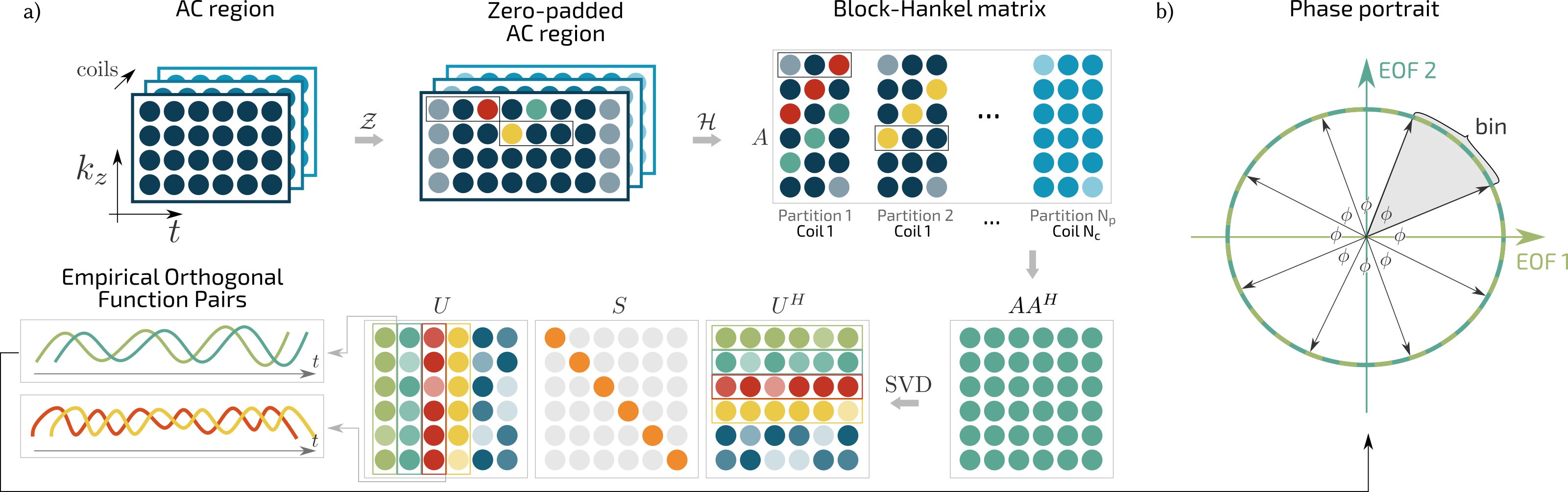
A schematic of the SSA-FARY procedure is depicted in Fig. 1a. In contrast to conventional (multivariate) SSA, we first zero-pad () the second dimension of the AC data to obtain matrix of size [],
| (7) |
Next, we construct a Block-Hankel calibration matrix
| (8) |
of size []. Here, the Hankelization operator slides a window of size [] through channel of the zero-padded AC data and takes each block to be a row in the -th column of the calibration matrix. This operation is similar to the construction of the calibration matrix in ESPIRiT [41].
We decompose using an SVD
| (9) |
and consider of size [] as the orthonormal basis that consists of the Empirical Orthonormal Functions (EOFs) , . The principle components are given by
| (10) |
The expansion of , or , in the basis then reads
| (11) |
where iterates through the temporal samples, through the channels and is the index inside the sliding window. The EOFs can be considered as data-adaptive weighted moving averages of the original time series , with being the data-adaptive filters [29, 42],
| (12) |
| (13) |
In fact, the columns of can bee seen as a complete eigenfilter decomposition of the original time series [43]. These filters act as data-adaptive band-pass filters with a frequency bandwidth given by
| (14) |
where is the sampling rate [44, 45]. Harris and Yuan showed in [42] for the univariate case that a periodic oscillation contained in the data lead to an even and odd filter. The application of these filters to the original time series constitutes for each oscillation one EOF which is in phase and one which is in quadrature to the original oscillation, respectively.
Vautard et al. [29] proposed another interpretation of the EOFs considering the minimization problem
| (15) |
The solution of eq. (15) is , thus the EOFs can be obtained by a local least-squares fit of the k-th principle component to the original time series. This locality, determined by the window size , distinguishes SSA-FARY from classical PCA, which does not take the temporal past and future of a sample into account. In fact, PCA is a special case of SSA-FARY with ,
| (16) |
In conventional SSA, i.e. where no zero-padding is applied, the EOFs are of reduced length . Thus, the exact correspondence in time is lost, which inhibits their use as self-gating signal. In contrast, the EOFs in SSA-FARY preserve the length of the original time series and can directly be used for self-gating, similar to the eigenvectors in PCA. In distinction to PCA, the EOFs in SSA(-FARY) capture temporal oscillations via oscillatory pairs [28]. In particular, if two consecutive eigenvalues are nearly equal, the two corresponding EOFs are nearly periodic with the same period and in quadrature [46], which is a consequence of the filtering property of SSA-FARY [42]. To ensure a proper separation the singular values of different EOF pairs should be distinct, which is called the strong separability condition [47] and usually fulfilled for our application.
These pairs can be seen as the data-adaptive equivalent to the sine-cosine pairs of Fourier analysis [48]. A single EOF-pair might suffice for the analysis of nonlinear and inharmonic oscillations, as it automatically locates intermittent oscillatory regions. In contrast, classical spectral analysis would require a large amount of harmonics or subharmonics of the fundamental period [29, 49].
Comments
The EOF is also the k-th left eigenvector of the [] real-symmetric cross-covariance matrix
| (17) |
Depending on the number of acquired spokes and partitions, computing the eigen-decomposition of is usually more efficient than computing the SVD of .
In contrast to the parameter-free PCA, for SSA we must define a window size . To long-range correlations in time, should be large, which - as a trade-off - results in a lower degree of statistical confidence [49]. Vautard et al. [29] showed that SSA can resolve oscillations best when the periods are shorter than the window size . In our study, the window size proofed to be a robust choice for most measurements, independently of the utilized sequence, and this value was chosen as the default. More information on the choice of the window size is given in the Methods and Discussion section.
The fundamental concept behind the use of a temporal window is Taken’s delay embedding theorem [26], one of the backbones of chaotic dynamical system analysis. Instead of considering each temporal sample individually and isolated from other time points, so called time-delay coordinates are constructed by embedding the samples in a higher-dimensional space with embedding dimension . Consequently, each time point is represented by a time-delay coordinate vector, which comprises not only the sample of the respective time but also its temporal past and future. It is therefore a natural choice to pick an odd value for in order to incorporate the same amount of past and future information.
Towards the beginning and the end of a time series this embedding can no longer be constructed due to lack of past or future samples, respectively. There are two strategies to overcome this limitation: 1.) Time-delay coordinates are constructed for the central samples only, which means that samples would be discarded from future processing. 2.) samples are zero-padded on both ends of the time series, which comes at the expense of increased inaccuracy for the marginal samples of the time series. However, for the second approach no samples have to be discarded and through the symmetric zero-padding the time-delay coordinates remain in sync with the actual temporal evolution of the signal. In this manuscript, the second approach is used.
2.3 Binning
The myocardium shows different behavior for contraction and expansion, so usually the entire cardiac cycle is divided into multiple distinct bins to accurately resolve the temporal motion. For respiratory gating it is usually assumed that inspiration and expiration do not have to be distinguished [50, 20, 16]. However, various studies reveal that respiratory motion is heavily subject-dependent and exhibits a strong variability as well as hysteresis, which affects the global position of the myocardium [51, 52, 53, 54]. Hence, inspiration and expiration should be distinguished to properly resolve the effects of breathing motion on the heart.
Since SSA-FARY yields EOF quadrature pairs that capture the phase information of periodic oscillations, binning is straight-forward for both cardiac and respiratory motion: The phase portrait, i.e. the amplitude-amplitude scatter plot, of an EOF pair is divided into circular sectors with central angle . The samples are then binned according to their respective circular sector, see Fig. 1b.
3 Methods
3.1 Numerical Simulations
We compare the capability of PCA and SSA-FARY in extracting and separating oscillatory signals in simple numerical simulations.
The signals we want to extract are two frequency-modulated sinusoids
| (18) |
| (19) |
with
| (20) |
| (21) |
which account for frequency variations. To simulate various channels , we use a weighted sum
| (22) |
To spoil the composite signals , we add Gaussian white noise with standard deviation , or an oscillatory spell from time to time ,
| (23) |
or an exponential trend
| (24) |
to all channels, which yields
| (25) |
We analyze the time-series , and using PCA and SSA-FARY with window size . Note, that the aim of this numerical experiment is to demonstrate the general benefits of SSA-FARY over PCA for the analysis of time series, and not to simulate cardiac and respiratory motion in the most accurate way. We therefore did not include the modeling of a more complex frequency variability or motion signal shapes. More details on the simulation are provided in the appendix.
3.2 In Vivo experiments
All measurements were performed on a Skyra 3T scanner (Siemens Healthcare GmbH, Erlangen, Germany) using 30 channels of a thorax and spine coil. Gradient delay correction was performed using RING [55, 56]. The AC data was corrected using the orthogonal projection with . In the following, the AC data’s real and imaginary part are treated as individual channels. The field of view in all experiments was at base resolution . All presented experiments were performed on volunteers with no known diseases, who gave written informed consent. All SOS measurements were performed on different volunteers. The study had received approval from the local ethics committee.
Sequence Design, Auto-Calibration and Reconstruction
We utilize a radial bSSFP sequence for the single-slice measurement, an RF-spoiled gradient-echo sequence with randomized RF spoiling [57] for the SMS measurement and a radial bSSFP sequence with undersampling in direction [58] for the SOS measurement. To obtain maximum k-space coverage and thus improved image quality [59, 60], the projection angle is increased in each shot about the seventh tiny golden angle [61]. For the SMS and SOS measurements, the partitions are acquired in an interleaved fashion, i.e. one spoke is recorded for each partition before the next in-plane spoke of a partition is acquired.
For single-slice imaging, the central sample of all spokes is used for auto-calibration. For SMS, more AC data is available as not only a single sample but the central line along the () direction can be utilized.
Inspired by [58], we make use of variable-density -undersampling for the SOS acquisition. From the total number of 14 partitions, the central 6 partitions are always acquired and the corresponding central line is used for auto-calibration. The remaining 8 partitions are undersampled by a factor of 4. This center-dense sampling scheme does not only increase the temporal resolution of the AC data but also improves the image quality [62].
For self-gating with PCA and SSA-FARY as well as for imaging reconstruction we use BART [63]. Image reconstruction is performed using combined parallel imaging and compressed sensing (PICS) [64] applying the alternating direction method of multipliers (ADMM) [65] with in-plane wavelet-regularization on the spatial dimensions and total variation (TV) on the cardiac and respiratory dimension [20, 66]. For SOS imaging, we additionally apply TV regularization in slice direction. The coil sensitivities for the single-slice and SMS measurements are generated using radial ENLIVE allowing two maps [3, 60, 67, 41]. To reduce the memory demand we allow only one map in the SOS reconstruction. We apply coil compression [68, 69] to reduce the number of coils to 13 for single-slice and SMS, and 10 for SOS imaging and perform the calibration of the sensitivities using a lower resolution.
The SSA-FARY gating signals is distributed into 25 cardiac and 9 respiratory bins for image reconstruction. Although not always necessary, we standardly perform an additional detrending of the EOFs using a moving average filter of length . This further improves the binning accuracy of SSA-FARY by removing a possibly remaining residual trend.
In the spirit of reproducible research, code and data to reproduce the experiments are made available on Github.111https://github.com/mrirecon/SSA-FARY
Single-slice imaging
We perform a second free-breathing bSSFP scan (TE/TR = , flip angle ) with slice-thickness of the human heart in short-axis view and use the first 30 seconds of data for further analysis and image reconstruction. The full second scan is used for a gridding reconstruction in Supplementary Material chapter II. We furthermore conduct an ECG-triggered CINE bSSFP breath-hold scan of the same slice (TE/TR = , flip angle , slice-thickness ).
We compare the principal motion signals using PCA and SSA-FARY with window size , which covers a period of about .
SMS imaging
We perform a 60 second free-breathing SMS RF-spoiled gradient-echo scan (TE/TR = , flip angle ) with three simultaneously acquired slices in short-axis view. The slice thickness is and the slice gap . We use SSA-FARY with window size , which covers a period of about . We perform a joint reconstruction of all slices using binning based on SSA-FARY. To evaluate the accuracy of SSA-FARY, we compare the SSA-FARY respiration quadrature-signals of the complete time series with the breathing pattern extracted from a pneumatic respiratory belt (Siemens Healthcare GmbH, Erlangen, Germany) and a real-time reconstruction [60, 70].
SOS imaging
We measure 8 volunteers and on each we perform a free-breathing three-minute radial SOS bSSFP scan (TE/TR = , flip angle ) with fourteen partitions in short-axis view and slice thickness . By default we use SSA-FARY with window size , which covers a period of about . For one volunteer the respiratory EOF pair revealed highly irregular breathing with occasional breath-holds of up to and for another volunteer the cardiac EOF pair showed a pronounced frequency variation. To improve the gating accuracy in these two cases, we determined another respiratory EOF pair using window size and another cardiac EOF pair using window size , respectively.
To evaluate the precision of the cardiac gating with SSA-FARY, we analyze the SSA-FARY signal in comparison to the simultaneously acquired ECG trigger using a Python 3 script. Therefore, we define a synthetic trigger point when the phase related to the orthogonal cardiac SSA-FARY quadrature pair experiences a zero-phase crossing. Since the global phase-offset of the quadrature pair is arbitrary, we correct the synthetic SSA-FARY trigger by a constant shift using the average distance to the ECG trigger. We then compute the standard deviation and standard error of the corrected SSA-FARY trigger to the ECG trigger.
Moreover, we acquire the same slices using a conventional ECG-triggered breath-hold CINE single-slice stack bSSFP measurement with Cartesian read-out (TE/TR = , flip angles depending on the Specific Absorbtion Rate (SAR) limits between and ) and cardiac bin size . The patient dependent measurement time is around . We compare the end-diastolic and end-systolic left-ventricular blood-pool area of a mid-ventricular slice to the SSA-FARY based reconstruction using ImageJ.
4 Results
Numerical simulations
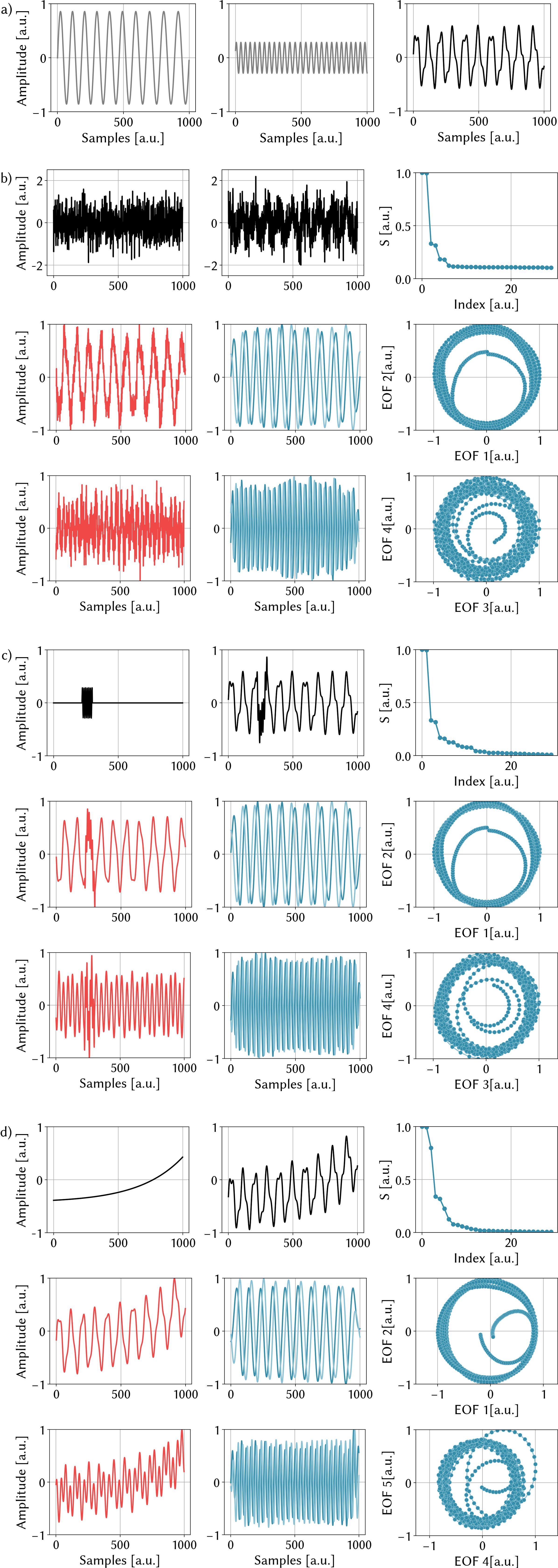
Fig. 2 depicts the results of the numerical simulations. PCA is able to extract, at least essentially, the shape of the two oscillations and from and . However, both the noise and the oscillation spell are still evident in the resulting eigenvectors and corrupt the signal. PCA fails to produce a useful result for . While oscillation is present in two principle eigenvectors, oscillation is not distinctly separated in any of the eigenvectors.
In contrast, SSA-FARY extracts the oscillation signals with almost no spoiling residuals in all three investigated cases. Only at the borders deviations from the ideal signal can be observed. Notably, SSA-FARY does not only yield a one-dimensional signal of the temporal evolution of an oscillation, but preserves the phase information by quadrature pairs, as can be appreciated from the amplitude-amplitude plots. The two EOFs corresponding to the same pair have very similar singular values. In the scree plot of Fig. 2 b) and c), the first plateau corresponds to EOF 1 and 2, and the second plateau belongs to EOF 3 and 4. In Fig. 2 d), the first two plateaus correspond to EOF 1 and 2, and to EOF 4 and 5. Hence, SSA-FARY does not mix the trend into the oscillations but creates an additional EOF to account for it.222In Supplementary Material Fig. 1-3 we provide results for simulations with different noise variance and trend and spell amplitudes, as well as a different frequency variation. More information on these figures is provided in chapter I of the supplementary document.
Single-slice imaging
For each coil, Fig. 3 depicts the DC component of 100 consecutive spokes before and after the data correction using the orthogonal projection. Before correction some coils exhibit pronounced oscillations with approximately 15 samples per period. As we have used the seventh tiny golden angle () the oscillations period of 15 samples corresponds to (see eq. (1)). Hence, the oscillation period in the AC data is linked to the period of the projection angle. By removing this frequency and the higher-order harmonics these oscillations can be completely eliminated.
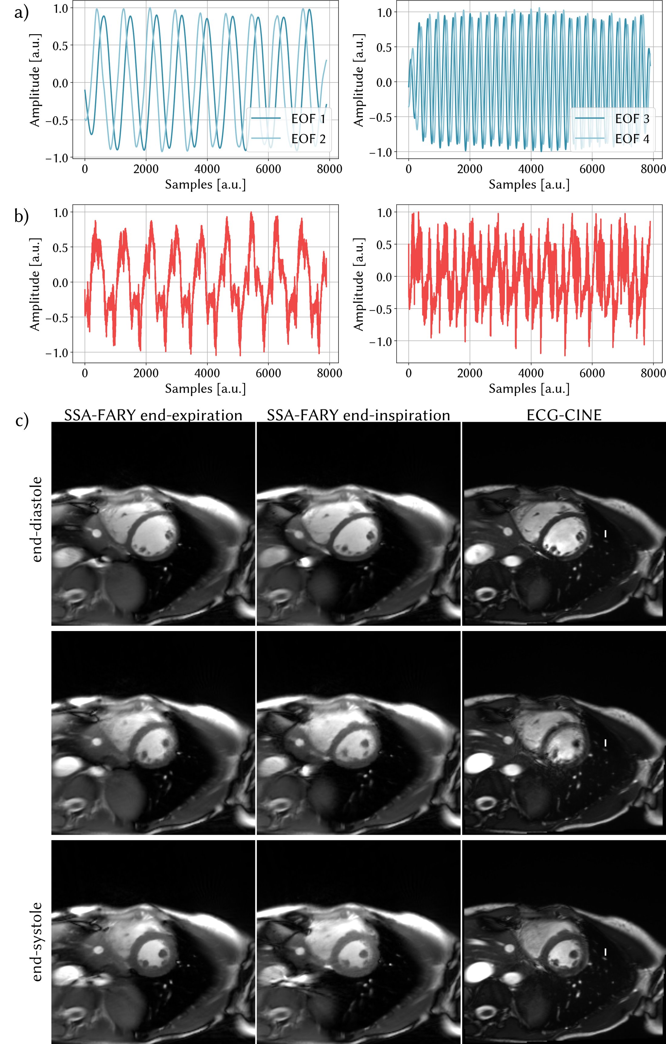
Fig. 4 shows the self-gating signals generated with PCA and SSA-FARY. In SSA-FARY, the first two EOFs represent respiratory motion and the third and fourth EOF cardiac motion. The EOFs of the pairs are in quadrature, respectively. Both the cardiac and the respiratory phases are well separated. In contrast, PCA cannot fully extract and separate the signals as respiratory and cardiac motion are superposed and heavily spoiled by noise.
Fig. 4c shows six representative images of the SSA-FARY-gated reconstruction. Depicted are from bottom to top the end-systolic, an intermittent and the end-diastolic frame for end-expiration and end-inspiration, respectively. For comparison, we also show the result of the ECG-triggered CINE breath-hold scan.
In Supplementary Material chapter II we present the results of a conventional gridding reconstruction of the full 72 second measurement gated with SSA-FARY.333Supplementary Material Fig. 4 shows the SSA-FARY and PCA gating signals of the 72 second scan. Moreover, a gridding reconstruction for three different cardiac phases is depicted and the results of a breath-hold and an ECG-gated CINE scan are shown for comparison.
In Supplementary Material chapter III we present a similar experiment with a RF-spoiled gradient-echo sequence.444Supplementary Material Fig. 5 shows the effect of the proposed correction on the AC region. Supplementary Material Fig. 6 shows the self-gating signals determined with SSA-FARY and PCA. Furthermore, six representative frames of the SSA-FARY-gated reconstruction for different respiratory and cardiac motion states are depicted.
SMS imaging
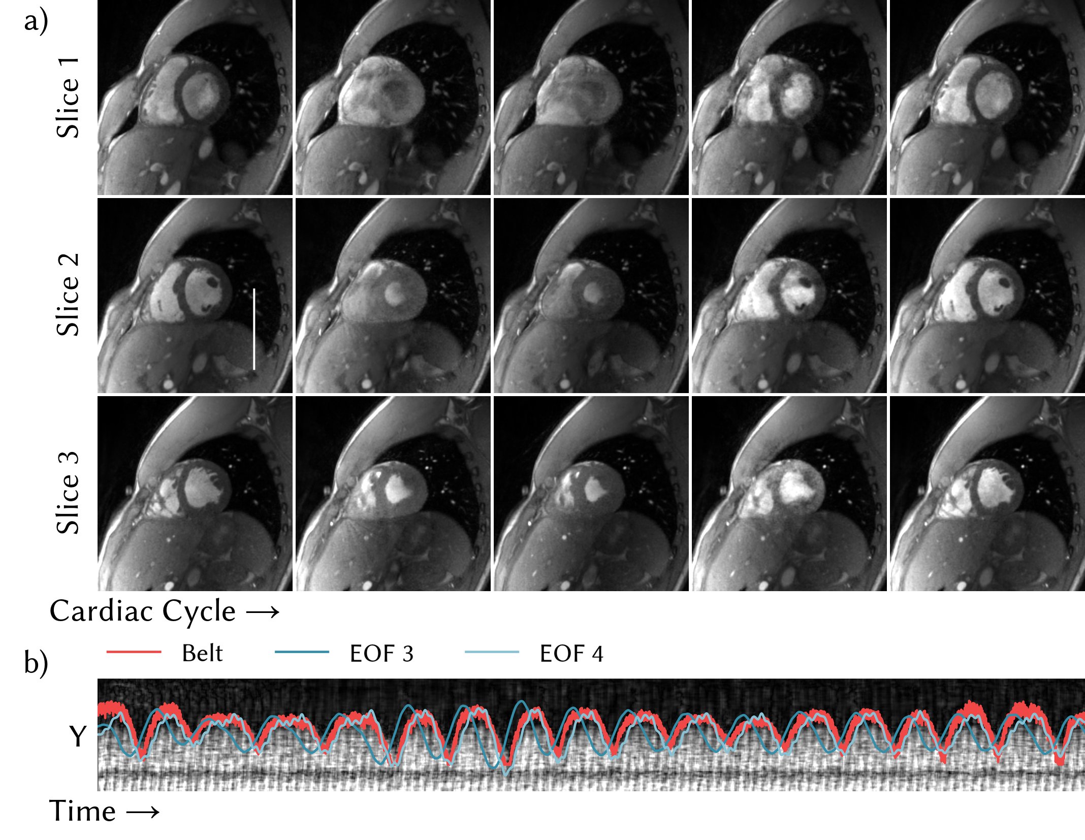
Fig. 5a shows 5 out of 25 cardiac phases for all three slices in end-expiration. The different systolic and diastolic phases are well resolved.
The background of Fig. 5b shows the temporal evolution of a line extracted from an SMS-NLINV real-time reconstruction of the full time series. The line was placed in slice two in vertical direction such that the actual motion of the diaphragm can be observed. This diaphragmatic motion is linearly related to the translation of the heart during breathing [71]. On top of the background image, we have plotted the respiratory EOF quadrature pair obtained from SSA-FARY as well as the signal provided by the respiratory belt. For the purpose of comparison, the motion signals were scaled according to the amplitude of the diaphragm motion in the background image.
One of the EOFs (light blue) coincides very well both in amplitude and phase with the temporal evolution of the diaphragm. This is in line with the filtering interpretation of SSA-FARY, which states that one EOF of the quadrature pair is in phase with the related underlying motion, whereas the other EOF (dark blue) constitutes the quadrature signal. The in-phase EOF is furthermore in good agreement with the motion signal provided by the respiratory belt.
The presented volunteer shows a largely periodic breathing pattern. In Supplementary Material chapter IV we present the results of the same experiment on another volunteer, which happend to exhibit a highly irregular respiration pattern during measurement.555 In Supplementary Material Fig. 7 we provide results of the same experiment conducted on a different volunteer. We depict 5 cardiac phases for all three slices, as well as a comparison between the SSA-FARY respiratory self-gating signal, the respiratory belt and the diaphragm motion extracted from a real-time reconstruction.
SOS imaging
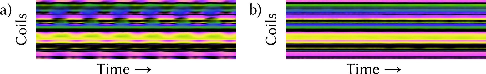
Fig. 6a depicts a zoomed view on EOFs representing respiratory and cardiac motion for different window sizes. For window size , which - considering the undersampling scheme - covers a period of , respiratory and cardiac motion are not fully separated and appear superposed in one EOF for respiratory and one EOF for cardiac motion. In contrast, for the proposed window size () the motion signals are well separated. Then again, for () a signal loss can be observed in the cardiac EOFs. Fig. 6b shows one respiratory EOF and one cardiac EOF for the windows , and , covering periods from to . All signals are in good agreement. The corresponding pairing-components of the EOFs show similar behavior and are therefore not depicted. Fig. 6c presents end-diastolic and end-systolic frames for three out of fourteen slices in end-expiration. All respiratory and cardiac states are well separated, the cardiac wall and the diaphragm are sharply resolved. Note, however, that some slices at the fringe of the slab have low signal intensity due to an unoptimized excitation profile. The image quality is comparable to the CINE reconstruction Fig. 6d, although the latter tends to be sharper. Due to the higher flip-angle, which is restricted by SAR limitations in volumetric sequences, the CINE images possess a better blood myocardium contrast.

For the different volunteers, Table (1) shows the average heart-rate , its standard deviation , the standard deviation of the synthetic SSA-FARY trigger to the ECG trigger and the end-diastolic and end-systolic left-ventricular blood-pool area of a mid-ventricular slice for CINE and SSA-FARY.
For imaging on a 3T system an insufficient shim can lead to banding artifacts. Measurements with bandings affecting the heart could not immediately be noticed and repeated as the reconstruction was performed offline. Therefore, these measurements were discarded for which the analysis of one volunteer is omitted.
The observed average heart rates range from ( bpm) to ( bpm) with different heart rate variabilities. For the given SOS acquisition with 14 partitions (6 AC lines and undersampling factor of 4), the temporal resolution of the SSA-FARY trigger is . The standard deviation of the SSA-FARY trigger to the ECG trigger, , is of similar size. Hence, the SSA-FARY trigger is in good agreement with the ECG signal and also matches the temporal resolution of the ECG-CINE acquisition.
The areas of the chosen mid-ventricular slices are comparable for ECG-CINE and SSA-FARY, particularly for end-diastole the difference lies mostly in the lower single-digit percent range, whereas a larger uncertainty can be observed for end-systole.
Volunteer V6 exhibits a highly erratic breathing pattern and volunteer V7 possesses a strongly irregular heartbeat and furthermore unintentionally yawned three times during the measurement. Still, SSA-FARY can provide satisfying results as Table 1 and the figures in the Supplementary Material show.666Supplementary Material Fig. 8 and 9 display the SSA-FARY gating signal, representative frames of the SSA-FARY-based image reconstruction and the corresponding CINE reconstructions for volunteers V6 and V7. More information on the figures is provided in chapter V of the supplementary document.
| Volunteer | [] | [] | [] | Diastole [] | Systole [] | ||||
|---|---|---|---|---|---|---|---|---|---|
| ECG | SSA-FARY | Err. [] | ECG | SSA-FARY | Err. [] | ||||
| V1 | 0.910(4) | 0.057(3) | 23(1) | 2254 | 2222 | 1.4 | 1068 | 1017 | 4.8 |
| V2 | 1.380(3) | 0.0541(2) | 14.7(7) | 1536 | 1647 | 7.2 | 573 | 706 | 23.2 |
| V3 | 0.979(2) | 0.0245(1) | 28(2) | 1911 | 2161 | 13.1 | 1072 | 1168 | 11.0 |
| V4 | 1.245(3) | 0.045(2) | 23(1) | 1998 | 1956 | 2.1 | 866 | 961 | 11.0 |
| V5 | 0.955(4) | 0.056(3) | 19(1) | 2348 | 2380 | 1.4 | 1005 | 1179 | 17.3 |
| V6∗ | 1.195(7) | 0.103(5) | 34(2) | 2244 | 2220 | 1.1 | 1351 | 1407 | 4.1 |
| V7∗∗ | 1.08(1) | 0.129(7) | 27(1) | 3398 | 3314 | 2.5 | 2060 | 1930 | 6.3 |
For all in vivo experiments, we have attached representative movies as Supplementary Material.777The files Mov1-14 of the Supplementary Material show representative movies of all in vivo reconstructions. More information on the movies is provided in chapter VI of the supplementary document.
5 Discussion
We introduced a novel dimensionality reduction method dubbed ”SSA-FARY”, which is based on Singular Spectrum Analysis and showed that the proposed technique can successfully recover the cardiac and respiratory signal from the AC data of single-slice, SMS and SOS MRI measurements. Moreover, we have proposed an extended orthogonal projection to correct for system imperfections in the AC data.
AC correction
The reasons for the oscillations in the AC data are many fold and according to our experience cannot be eliminated completely by techniques that correct for trajectory errors only [72, 73]. Particularly for bSSFP sequences, eddy current related dephasing of spins additionally compromises the data [74, 75], although this effect should be rather small for the tiny golden angle [61].
Zhang et al. [76] find this to be particularly problematic for 3D bSSFP imaging on a 3T system and propose to eliminate these measurement errors by averaging over the central five samples of each spoke. However, we found this to produce even more oscillations in the AC data, which requires additional filtering. In contrast, the orthogonal projection used here can remove most of the signal perturbations directly. For constant increments of the projection angle, the correction can be thought of as a set of sharp band-stop or notch filters corresponding to higher-order harmonics of a base frequency, which can be calculated from the increment of the projection angle.
Strictly speaking, the AC correction is not mandatory for SSA-FARY as without filtering these spurious oscillations appear as additional EOFs. However, as these oscillations usually manifest distinctly in the AC region, the corresponding EOFs often possess the highest singular values. Consequently, they dominate the result of eq. (15) which reduces the significance and accuracy of the components of interest, i.e. cardiac and respiratory motion, and complicates the analysis. This can be easily avoided by using the proposed orthogonal projection, which corrects for first-order system imperfections.
Alternatively, advanced techniques to measure the trajectory error [77, 78] or higher-order system imperfection corrections could be utilized to account for the oscillations in the AC region [79, 80]. Still, these approaches require additional hardware and/or sequence modifications, which limits their accessibility.
SSA-FARY
The presented dimensionality reduction technique for time-series SSA-FARY can be considered a PCA applied to a time-delayed embedding of the AC data to exploit the locally low-rankness of dynamic time series. The Block-Hankel matrix (eq. (8)) consists of shifted segments of the original time series. Its covariance matrix (eq. (17)) is an array of scalar products specifying the correlation of all pairs of multi-channel segments in the embedding space. The considerable redundancy in the correlations of the segments in the presence of (quasi) repetitive oscillations, e.g. cardiac and respiratory motion, causes to have low-rank. By exploiting not only spatial but also these temporal correlations, SSA-FARY performs better in recognizing temporal patterns than classical PCA and allows the separation of trend, oscillations and noise from the signal. This was successfully demonstrated on numerical simulations of superposed and spoiled sinusoidal time series. In the actual in vivo measurements the respiratory and cardiac motion could be detected and clearly separated for all investigated sequence types.
To yield comparable results, methods like classical PCA must be combined with various pre- and post-processing techniques such as coil-selection or coil-clustering [23], (iterative) band-pass filtering [50] and signal smoothing [20], which - especially for small AC regions - may be unstable and demand further manual tuning. By contrast, in SSA-FARY these steps are implicitly integrated and therefore surplus to requirement. Moreover, since SSA-FARY preserves phase information by producing quadrature pairs it allows for direct binning, which also renders the otherwise mandatory peak detection obsolete [10].
We demonstrated the high quality of the SSA-FARY gating signals by comparison with a real-time reconstruction, a respiratory belt and ECG triggers. Moreover, at free breathing and at a considerably lower acquisition time SSA-FARY achieved a reconstruction quality that comes close to the results of the ECG-triggered CINE breath-hold scans. The analyzed left-ventricular blood-pool area of SSA-FARY reconstructions mostly corresponds well to the CINE results for end-diastole, whereas larger uncertainties were found for end-systole. Here, because the left-ventricular blood-pool area is significantly decreased compared to end-diastolic states, any deviation will result in larger relative errors. One reason might be that due to the high acceleration factor the short end-systolic phase is not perfectly resolved. In addition, some discrepancy between a breath-hold scan and a gated free-breathing scan is expected, since it cannot be guaranteed that the selected respiratory bins exactly matches the anatomical state of the breath-hold scan.
As the aim of this manuscript was the introduction of the self-gating technique, we did not fully optimize the sequence and reconstruction parameters, particularly the number of cardiac and respiratory bins, the regularization values of the ADMM and the undersampling scheme of the SOS sequence. The parameter tuning and the setup of a clinically applicable protocol is left for future investigations.
In single-slice imaging we only use a single sample per time step for auto-calibration and despite the proportionally large window size, which reduces statistical significance, SSA-FARY yields reliable results. Still, SSA-FARY tends to be more resilient when multiple partitions are used and thus more AC data is available, as in SMS or SOS experiments, or when more samples relative to the window size are used for auto-calibration. For SMS or SOS imaging a bSSFP sequence is recommended since for RF-spoiled gradient-echo imaging a loss of contrast in systolic phases can occur due to pre-saturated blood flowing in from other slices, see Fig. 5. Note, however, that bSSFP sequences suffer from SAR limitations due to the increased flip-angle of the RF pulse and are prone to banding artifacts when no proper shimming is conducted.
Due to the zero-padding operation, eq. (7), and the subsequent Hankelization, eq. (8), the first and last samples in the SSA-FARY EOFs suffer from slight approximation errors. Still, for all presented experiments and analysis we did not discard these samples.
Occasionally, the trend was not completely separated from the EOFs for cardiac and respiratory motion, which we fixed by standardly using a moving average filter. The reason for the incomplete separation of trend can be understood by considering eq. (14), which relates the window size to the frequency bandwidth of the eigenfilters generating the EOFs . Our default choice of window size and sampling rate corresponds to for all measurements and sequences. If we choose too small, the EOFs capture a wider range of frequencies, which can result in a mixing of trend and oscillations. Similarly, if the respiration frequency (usually ) and cardiac frequency (usually ) happen to be spectrally close to one another, a very small window and the corresponding large frequency pass-band of the filters can hinder a proper separation, as it is the case in Fig. (6a), ). Then again, if we choose a very large , the frequency response of the filters can be too narrow. Thus, possible frequency variations in the cardiac and respiratory motion can no longer be captured by a single (band-limited) EOF, which results in signal voids and/or the generation of additional EOFs representing higher order harmonics. Detecting these related EOFs corresponds to the ’Grouping’ step of conventional SSA [81]. In the cardiac signal of Fig. (6a) such a signal void caused by a cardiac frequency variation of can be observed for , whereas the signal can still be adequately captured with . As a summary, we found to be a robust choice and we propose to choose the window size accordingly using eq. (14).
The computational bottle-neck of SSA-FARY is the SVD of of size . Especially for single-slice imaging, the window size required to obtain and the corresponding number of AC samples to obtain good results is relatively large. Hence, the decomposition of is rather time-consuming. Nevertheless, there are approaches to significantly speed up the decomposition stage [82, 83].
SSA-FARY reliably detected the EOF pairs corresponding to cardiac and respiratory motion, which for RF-spoiled gradient echo measurements usually possess the highest singular values. It is, however, not determined that the two largest components belong to the cardiac or the respiratory motion. For bSSFP sequences, which are generally more prone to system imperfections, we frequently found other components such as trends to have high singular values, too. Although for this study the components used for gating were chosen by visual inspection of the EOFs, it is fairly simple to automatize the assignment using a frequency analysis.
If one finds the separation of SSA-FARY to work insufficiently, a variation of the window size usually helps to recover a suitable gating result. Still, for patients with strong cardiac or respiratory frequency variations, highly non-periodic respiratory motion or arrhythmia the results of the presented SSA-FARY method might still be insufficient. In this case various promising extensions of SSA(-FARY) exist to improve the results, e.g. ’Nonlinear Laplacian Spectral Analysis’, ’Sliding SSA’, ’Oblique SSA’, ’Nested SSA’ and their combinations [84, 85, 47].
Outlook
The property of SSA-FARY to not only reliably separate cardiac and respiratory motion but also to extract the trend in data, suggests further applications. In dynamic contrast-enhanced MRI, SSA-FARY could replace spline-fitting [20] for separating motion and contrast enhancement. Furthermore, preliminary results suggest that the T1 decay in inversion recovery sequences is detected as an individual component and separated from the motion signals, which would enable the simultaneous reconstruction of parameter maps and self-gated anatomical motion [86].
Last but not least we want to mention that the zero-padding approach used in SSA-FARY is not limited to self-gated MRI but turns multi-variate SSA into a general dimensionality reduction method, which might be useful for many other problems related to time-series analysis.
6 Conclusion
We have introduced a novel SSA-based dimensionality reduction method called SSA-FARY. Its intuitive approach, the easy implementation and its capability to separate cardiac and respiratory motion as well as trend makes it a promising approach for MRI self-gating, particularly when it is combined with efficient data acquisition schemes and a state-of-the-art image reconstruction technique.
7 Acknowledgement
The orthogonality projection to correct the AC data was originally conceived by Dr. Anthony G. Christodoulou (Biomedical Imaging Research Institute, Cedars-Sinai Medical Center). We extended it by including the higher-order harmonics.
Supported by the DZHK (German Centre for Cardiovascular Research), the Physics-to-Medicine Initiative Göttingen (LM der Niedersächsischen Vorab), the DFG (German Research Foundation) under grant UE 189/1-1, and the Studienstiftung des deutschen Volkes. We gratefully acknowledge the support of the NVIDIA Corporation with the donation of one NVIDIA TITAN Xp GPU for this research.
Appendix A Details for Numerical Simulations
Here we present the values for the variables used in the numerical simulation (Fig. 2). The total duration consists of discrete samples. The other parameters can be found in Table 2.
| Variable | Value |
|---|---|
References
- [1] A. B. Kerr, J. M. Pauly, B. S. Hu, K. C. Li, C. J. Hardy, C. H. Meyer, A. Macovski, and D. G. Nishimura, “Real-time interactive mri on a conventional scanner,” Magn. Reson. Med., vol. 38, no. 3, pp. 355–367, 1997.
- [2] P. C. Yang, A. B. Kerr, A. C. Liu, D. H. Liang, C. Hardy, C. H. Meyer, A. Macovski, J. M. Pauly, and B. S. Hu, “New real-time interactive cardiac magnetic resonance imaging system complements echocardiography,” J. Am. Coll. Cardiol., vol. 32, no. 7, pp. 2049–2056, 1998. http://www.sciencedirect.com/science/article/pii/S0735109798004628
- [3] M. Uecker, S. Zhang, and J. Frahm, “Nonlinear inverse reconstruction for real-time MRI of the human heart using undersampled radial FLASH,” Magn. Reson. Med., vol. 63, no. 6, p. 1456–1462, 2010.
- [4] M. Uecker, S. Zhang, D. Voit, A. Karaus, K.-D. Merboldt, and J. Frahm, “Real-time MRI at a resolution of 20 ms,” NMR Biomed., vol. 23, no. 8, pp. 986–994, 2010.
- [5] R. L. Ehman, M. McNamara, M. Pallack, H. Hricak, and C. Higgins, “Magnetic resonance imaging with respiratory gating: techniques and advantages,” Am. J. Roentgenol., vol. 143, no. 6, pp. 1175–1182, 1984.
- [6] Y. L. Liu, S. J. Riederer, P. J. Rossman, R. C. Grim, J. P. Debbins, and R. L. Ehman, “A monitoring, feedback, and triggering system for reproducible breath-hold mr imaging,” Magn. Reson. Med., vol. 30, no. 4, pp. 507–511, 1993. https://onlinelibrary.wiley.com/doi/abs/10.1002/mrm.1910300416
- [7] L. Guo, “Novel techniques in projection-based motion tracking in cardiac magnetic resonance imaging,” Ph.D. dissertation, Johns Hopkins University, 2017.
- [8] C. B. Higgins and H. Hricak, Magnetic resonance imaging of the body. Elsevier, 1987.
- [9] R. Rokey, R. E. Wendt, and D. L. Johnston, “Monitoring of acutely iii patients during nuclear magnetic resonance imaging: Use of a time-varying filter electrocardiographic gating device to reduce gradient artifacts,” Magn. Reson. Med., vol. 6, no. 2, pp. 240–245, 1988.
- [10] A. C. Larson, R. D. White, G. Laub, E. R. McVeigh, D. Li, and O. P. Simonetti, “Self-gated cardiac cine MRI,” Magn. Reson. Med., vol. 51, no. 1, pp. 93–102, 2004.
- [11] W. Kim, C. Mun, D. Kim, and Z. Cho, “Extraction of cardiac and respiratory motion cycles by use of projection data and its applications to nmr imaging,” Magn. Reson. Med., vol. 13, no. 1, pp. 25–37, 1990.
- [12] M. E. Crowe, A. C. Larson, Q. Zhang, J. Carr, R. D. White, D. Li, and O. P. Simonetti, “Automated rectilinear self-gated cardiac cine imaging,” Magn. Reson. Med., vol. 52, no. 4, pp. 782–788, 2004.
- [13] A. C. Larson, P. Kellman, A. Arai, G. A. Hirsch, E. McVeigh, D. Li, and O. P. Simonetti, “Preliminary investigation of respiratory self-gating for free-breathing segmented cine MRI,” Magn. Reson. Med., vol. 53, no. 1, pp. 159–168, 2005.
- [14] S. Uribe, V. Muthurangu, R. Boubertakh, T. Schaeffter, R. Razavi, D. L. G. Hill, and M. S. Hansen, “Whole-heart cine MRI using real-time respiratory self-gating,” Magn. Reson. Med., vol. 57, no. 3, pp. 606–613, 2007.
- [15] M. Buehrer, J. Curcic, P. Boesiger, and S. Kozerke, “Prospective self-gating for simultaneous compensation of cardiac and respiratory motion,” Magn. Reson. Med., vol. 60, no. 3, pp. 683–690, 2008. https://onlinelibrary.wiley.com/doi/abs/10.1002/mrm.21697
- [16] J. Paul, E. Divkovic, S. Wundrak, P. Bernhardt, W. Rottbauer, H. Neumann, and V. Rasche, “High-resolution respiratory self-gated golden angle cardiac MRI: comparison of self-gating methods in combination with k-t SPARSE SENSE,” Magn. Reson. Med., vol. 73, no. 1, pp. 292–298, 2015.
- [17] J. Pang, B. Sharif, Z. Fan, X. Bi, R. Arsanjani, D. S. Berman, and D. Li, “Ecg and navigator-free four-dimensional whole-heart coronary mra for simultaneous visualization of cardiac anatomy and function,” Magn. Reson. Med., vol. 72, no. 5, pp. 1208–1217, 2014. https://onlinelibrary.wiley.com/doi/abs/10.1002/mrm.25450
- [18] M. Kirby, Geometric Data Analysis: An Empirical Approach to Dimensionality Reduction and the Study of Patterns. John Wiley & Sons, Inc., 2000.
- [19] Z. Deng, J. Pang, W. Yang, Y. Yue, B. Sharif, R. Tuli, D. Li, B. Fraass, and Z. Fan, “Four-dimensional mri using three-dimensional radial sampling with respiratory self-gating to characterize temporal phase-resolved respiratory motion in the abdomen,” Magn. Reson. Med., vol. 75, no. 4, pp. 1574–1585, 2016. https://onlinelibrary.wiley.com/doi/abs/10.1002/mrm.25753
- [20] L. Feng, L. Axel, H. Chandarana, K. T. Block, D. K. Sodickson, and R. Otazo, “XD-GRASP: Golden-angle radial MRI with reconstruction of extra motion-state dimensions using compressed sensing,” Magn. Reson. Med., vol. 75, no. 2, pp. 775–788, 2016.
- [21] S. Rosenzweig, H. C. M. Holme, N. Scholand, R. N. Wilke, and M. Uecker, “Self-gated and real-time simultaneous multi-slice cardiac mri from the same acquisition,” in Proc. Intl. Soc. Mag. Reson. Med., vol. 26, Paris, 2018, p. 0209.
- [22] Y. Gao, Z. Zhou, F. Han, P. J. Finn, and P. Hu, “Improved respiratory motion self-gating in cardiovascular mri,” J. Cardiov. Magn. Reson., vol. 18, no. 1, p. P7, 2016. https://doi.org/10.1186/1532-429X-18-S1-P7
- [23] T. Zhang, J. Y. Cheng, Y. Chen, D. G. Nishimura, J. M. Pauly, and S. S. Vasanawala, “Robust self-navigated body mri using dense coil arrays,” Magn. Reson. Med., vol. 76, no. 1, pp. 197–205, 2016.
- [24] K. Fukunaga, Introduction to statistical pattern recognition. Elsevier, 2013.
- [25] N. Golyandina, V. Nekrutkin, and A. A. Zhigljavsky, Analysis of time series structure: SSA and related techniques. Chapman and Hall/CRC, 2001.
- [26] F. Takens, “Detecting strange attractors in turbulence,” in Dynamical Systems and Turbulence (Warwick 1980), vol. 898. Berlin, Heidelberg: Springer, Berlin, Heidelberg, 1981, pp. 366–381.
- [27] D. S. Broomhead and G. P. King, “Extracting qualitative dynamics from experimental data,” Physica D, vol. 20, no. 2-3, pp. 217–236, 1986.
- [28] R. Vautard and M. Ghil, “Singular spectrum analysis in nonlinear dynamics, with applications to paleoclimatic time series,” Physica D, vol. 35, no. 3, pp. 395–424, 1989.
- [29] R. Vautard, P. Yiou, and M. Ghil, “Singular-spectrum analysis: A toolkit for short, noisy chaotic signals,” Physica D, vol. 58, no. 1-4, pp. 95–126, 1992.
- [30] D. S. Broomhead and G. P. King, “On the qualitative analysis of experimental dynamical systems,” in Nonlinear Phenomena and Chaos, S. Sarkar, Ed. Bristol, England: Adam Hilger, 1986, pp. 113–144.
- [31] A. Hannachi, I. T. Jolliffe, and D. B. Stephenson, “Empirical orthogonal functions and related techniques in atmospheric science: A review,” Int. J. Climatol., vol. 27, no. 9, pp. 1119–1152, 2007. https://rmets.onlinelibrary.wiley.com/doi/abs/10.1002/joc.1499
- [32] K. Koelle, X. Rodó, M. Pascual, M. Yunus, and G. Mostafa, “Refractory periods and climate forcing in cholera dynamics,” Nature, vol. 436, no. 7051, p. 696, 2005.
- [33] I. A. Rezek and S. J. Roberts, “Stochastic complexity measures for physiological signal analysis,” IEEE Trans. Biomed. Eng., vol. 45, no. 9, pp. 1186–1191, 1998.
- [34] U. Kumar and V. Jain, “Time series models (grey-markov, grey model with rolling mechanism and singular spectrum analysis) to forecast energy consumption in india,” Energy, vol. 35, no. 4, pp. 1709–1716, 2010. http://www.sciencedirect.com/science/article/pii/S0360544209005416
- [35] C. L. Wu, K. Chau, and Y. Li, “Methods to improve neural network performance in daily flows prediction,” J. Hydrol., vol. 372, no. 1, pp. 80–93, 2009. http://www.sciencedirect.com/science/article/pii/S0022169409002182
- [36] H. Janssens, S. Hou, J. Jaeger, A.-R. Kim, E. Myasnikova, D. Sharp, and J. Reinitz, “Quantitative and predictive model of transcriptional control of the drosophila melanogaster even skipped gene,” Nat. Genet., vol. 38, no. 10, p. 1159, 2006.
- [37] L. Feng, L. Axel, L. A. Latson, J. Xu, D. K. Sodickson, and R. Otazo, “Compressed sensing with synchronized cardio-respiratory sparsity for free-breathing cine mri: initial comparative study on patients with arrhythmias,” J. Cardiov. Magn. Reson., vol. 16, no. 1, p. O17, 2014. https://doi.org/10.1186/1532-429X-16-S1-O17
- [38] S. Rosenzweig, N. Scholand, H. Holme, and M. Uecker, “Robust cardiac and respiratory self-gating using an adapted singular spectrum analysis (ssa-fari): Application to simultaneous-multi-slice imaging,” in Proc. Intl. Soc. Mag. Reson. Med., vol. 27, Montreal, 2019, p. 2444. http://indexsmart.mirasmart.com/ISMRM2019/PDFfiles/0445.html
- [39] S. Rosenzweig, N. Scholand, H. Holme, and M. Uecker, “Robust cardiac and respiratory self-gating using an adapted singular spectrum analysis,” in Proc. Soc. Cardiovasc. Magn. Reson., vol. 22, Bellevue, 2019, p. 549871. http://indexsmart.mirasmart.com/ISMRM2019/PDFfiles/0445.html
- [40] N. A. Campbell and W. R. Atchley, “The geometry of canonical variate analysis,” Syst. Biol., vol. 30, no. 3, pp. 268–280, 1981. http://dx.doi.org/10.1093/sysbio/30.3.268
- [41] M. Uecker, P. Lai, M. J. Murphy, P. Virtue, M. Elad, J. M. Pauly, S. S. Vasanawala, and M. Lustig, “ESPIRiT—an eigenvalue approach to autocalibrating parallel MRI: where SENSE meets GRAPPA,” Magn. Reson. Med., vol. 71, no. 3, pp. 990–1001, 2014.
- [42] T. Harris and H. Yuan, “Filtering and frequency interpretations of singular spectrum analysis,” Physica D, vol. 239, no. 20-22, pp. 1958–1967, 2010.
- [43] K. Kume, “Interpretation of singular spectrum analysis as complete eigenfilter decomposition,” Adv. Adapt. Data Anal., vol. 4, no. 04, p. 1250023, 2012.
- [44] M. C. Leles, A. S. Cardoso, M. G. Moreira, H. N. Guimarães, C. M. Silva, and A. Pitsillides, “Frequency-domain characterization of singular spectrum analysis eigenvectors,” in IEEE Intern. Symp. Signal Process. and Info. Tech. (ISSPIT). Limassol: IEEE, 2016, pp. 22–27.
- [45] S. Xu, H. Hu, L. Ji, and P. Wang, “Embedding dimension selection for adaptive singular spectrum analysis of eeg signal,” Sensors, vol. 18, no. 3, p. 697, 2018.
- [46] G. Plaut and R. Vautard, “Spells of low-frequency oscillations and weather regimes in the northern hemisphere,” J. Atmos. Sci., vol. 51, no. 2, pp. 210–236, 1994.
- [47] N. Golyandina and A. Shlemov, “Variations of singular spectrum analysis for separability improvement: non-orthogonal decompositions of time series,” Stat. Interface, vol. 8(3), pp. 277–294, 2015.
- [48] A. Groth and M. Ghil, “Multivariate singular spectrum analysis and the road to phase synchronization,” Phys. Rev. E, vol. 84, no. 3, p. 036206, 2011.
- [49] M. Ghil, M. R. Allen, M. D. Dettinger, K. Ide, D. Kondrashov, M. E. Mann, A. W. Robertson, A. Saunders, Y. Tian, F. Varadi, and P. Yiou, “Advanced spectral methods for climatic time series,” Rev. Geophys., vol. 40, no. 1, pp. 3–1–3–41, 2002. https://agupubs.onlinelibrary.wiley.com/doi/abs/10.1029/2000RG000092
- [50] J. Liu, P. Spincemaille, N. C. F. Codella, T. D. Nguyen, M. R. Prince, and Y. Wang, “Respiratory and cardiac self-gated free-breathing cardiac CINE imaging with multiecho 3D hybrid radial SSFP acquisition,” Magn. Reson. Med., vol. 63, no. 5, pp. 1230–1237, 2010.
- [51] K. Nehrke, P. Bornert, D. Manke, and J. C. Bock, “Free-breathing cardiac mr imaging: study of implications of respiratory motion—initial results,” Radiology, vol. 220, no. 3, pp. 810–815, 2001.
- [52] I. Burger and E. M. Meintjes, “Elliptical subject-specific model of respiratory motion for cardiac mri,” Magn. Reson. Med., vol. 70, no. 3, pp. 722–731, 2013.
- [53] P. Dasari, K. Johnson, J. Dey, C. Lindsay, M. S. Shazeeb, J. M. Mukherjee, S. Zheng, and M. A. King, “Mri investigation of the linkage between respiratory motion of the heart and markers on patient’s abdomen and chest: Implications for respiratory amplitude binning list-mode pet and spect studies,” IEEE Trans. Nucl. Sci., vol. 61, no. 1, pp. 192–201, 2014.
- [54] P. K. Dasari, A. Könik, P. H. Pretorius, K. L. Johnson, W. P. Segars, M. S. Shazeeb, and M. A. King, “Correction of hysteretic respiratory motion in spect myocardial perfusion imaging: Simulation and patient studies,” Med. Phys., vol. 44, no. 2, pp. 437–450, 2017.
- [55] S. Rosenzweig, H. C. M. Holme, and M. Uecker, “Simple auto-calibrated gradient delay estimation from few spokes using radial intersections (ring),” Magn. Reson. Med., vol. 81, no. 3, pp. 1898–1906, 2019. https://onlinelibrary.wiley.com/doi/abs/10.1002/mrm.27506
- [56] S. Rosenzweig, H. Holme, and M. Uecker, “Simple auto-calibrated gradient delay estimation from few spokes using radial intersections (ring) for interactive real-time mri,” in Proc. Intl. Soc. Mag. Reson. Med., vol. 27, Montreal, 2019, p. 445. http://indexsmart.mirasmart.com/ISMRM2019/PDFfiles/0445.html
- [57] V. Roeloffs, D. Voit, and J. Frahm, “Spoiling without additional gradients: Radial FLASH MRI with randomized radiofrequency phases,” Magn. Reson. Med., vol. 75, no. 5, pp. 2094–2099, 2016.
- [58] L. Feng, T. Zhao, H. Chandarana, D. K. Sodickson, and R. Otazo, “Motion-resolved golden-angle radial sparse mri using variable-density stack-of-stars sampling,” in Proc. Intl. Soc. Mag. Reson. Med., Singapore, 2016, p. 1091. http://archive.ismrm.org/2016/1091.html
- [59] Z. Zhou, F. Han, L. Yan, D. J. Wang, and P. Hu, “Golden-ratio rotated stack-of-stars acquisition for improved volumetric mri,” Magn. Reson. Med., vol. 78, no. 6, pp. 2290–2298, 2017. https://onlinelibrary.wiley.com/doi/abs/10.1002/mrm.26625
- [60] S. Rosenzweig, H. C. M. Holme, R. N. Wilke, D. Voit, J. Frahm, and M. Uecker, “Simultaneous multi-slice mri using cartesian and radial flash and regularized nonlinear inversion: Sms-nlinv,” Magn. Reson. Med., vol. 79, no. 4, pp. 2057–2066, 2018.
- [61] S. Wundrak, J. Paul, J. Ulrici, E. Hell, and V. Rasche, “A small surrogate for the golden angle in time-resolved radial mri based on generalized fibonacci sequences,” IEEE Trans. Med. Imag., vol. 34, no. 6, pp. 1262–1269, 2015.
- [62] B. Berman, Z. Li, M. Altbach, J. Galons, D. Martin, B. Dong, P. Sharma, B. Kalb, and A. Bilgin, “How to stack the stars: A variable center-dense k-space trajectory for 3d mri,” in Proc. Intl. Soc. Mag. Reson. Med., Salt Lake City, 2013, p. 3829. http://archive.ismrm.org/2016/1091.html
- [63] M. Uecker, F. Ong, J. I. Tamir, D. Bahri, P. Virtue, J. Y. Cheng, T. Zhang, and M. Lustig, “Berkeley advanced reconstruction toolbox,” in Proc. Intl. Soc. Mag. Reson. Med., vol. 23, Toronto, 2015, p. 2486.
- [64] K. T. Block, M. Uecker, and J. Frahm, “Undersampled radial MRI with multiple coils. Iterative image reconstruction using a total variation constraint,” Magn. Reson. Med., vol. 57, no. 6, p. 1086–1098, 2007.
- [65] S. Boyd, N. Parikh, E. Chu, B. Peleato, and J. Eckstein, “Distributed Optimization and Statistical Learning via the Alternating Direction Method of Multipliers,” Found. Trends Mach. Learn., vol. 3, no. 1, pp. 1–122, 2011.
- [66] J. Y. Cheng, T. Zhang, M. T. Alley, M. Uecker, M. Lustig, J. M. Pauly, and S. S. Vasanawala, “Comprehensive multi-dimensional mri for the simultaneous assessment of cardiopulmonary anatomy and physiology,” Sci. Rep., vol. 7, no. 1, p. 5330, 2017.
- [67] H. C. M. Holme, F. Ong, S. Rosenzweig, R. N. Wilke, M. Lustig, and M. Uecker, “ENLIVE: A Non-Linear Calibrationless Method for Parallel Imaging using a Low-Rank Constraint,” in Proc. Intl. Soc. Mag. Reson. Med., vol. 25, Honolulu, 2017, p. 5160. http://indexsmart.mirasmart.com/ISMRM2017/PDFfiles/5160.html
- [68] F. Huang, S. Vijayakumar, Y. Li, S. Hertel, and G. R. Duensing, “A software channel compression technique for faster reconstruction with many channels,” Magn. Reson. Imaging, vol. 26, no. 1, pp. 133–141, 2008. http://www.sciencedirect.com/science/article/pii/S0730725X07002731
- [69] M. Buehrer, K. P. Pruessmann, P. Boesiger, and S. Kozerke, “Array compression for mri with large coil arrays,” Magn. Reson. Med., vol. 57, no. 6, pp. 1131–1139, 2007. https://onlinelibrary.wiley.com/doi/abs/10.1002/mrm.21237
- [70] S. Rosenzweig, H. C. M. Holme, R. N. Wilke, and M. Uecker, “Simultaneous Multi-Slice Real-Time Imaging with Radial Multi-Band FLASH and Nonlinear Inverse Reconstruction,” in Proc. Intl. Soc. Mag. Reson. Med., vol. 24, Honolulu, 2017, p. 0518.
- [71] Y. Wang, S. J. Riederer, and R. L. Ehman, “Respiratory motion of the heart: kinematics and the implications for the spatial resolution in coronary imaging,” Magn. Reson. Med., vol. 33, no. 5, pp. 713–719, 1995.
- [72] N. Seiberlich, F. A. Breuer, M. Blaimer, K. Barkauskas, P. M. Jakob, and M. A. Griswold, “Non-cartesian data reconstruction using grappa operator gridding (grog),” Magn. Reson. Med., vol. 58, no. 6, pp. 1257–1265, 2007.
- [73] A. Deshmane, M. Blaimer, F. Breuer, P. Jakob, J. Duerk, N. Seiberlich, and M. Griswold, “Self-calibrated trajectory estimation and signal correction method for robust radial imaging using grappa operator gridding,” Magn. Reson. Med., vol. 75, no. 2, pp. 883–896, 2016.
- [74] O. Bieri, M. Markl, and K. Scheffler, “Analysis and compensation of eddy currents in balanced ssfp,” Magn. Reson. Med., vol. 54, no. 1, pp. 129–137, 2005.
- [75] O. Bieri and K. Scheffler, “Flow compensation in balanced ssfp sequences,” Magn. Reson. Med., vol. 54, no. 4, pp. 901–907, 2005. https://onlinelibrary.wiley.com/doi/abs/10.1002/mrm.20619
- [76] X. Zhang, G. Xie, N. Lu, Y. Zhu, Z. Wei, S. Su, C. Shi, F. Yan, X. Liu, B. Qiu, and Z. Fan, “3d self-gated cardiac cine imaging at 3 tesla using stack-of-stars bssfp with tiny golden angles and compressed sensing,” Magn. Reson. Med., vol. 81, no. 5, pp. 3234–3244, 2019. https://onlinelibrary.wiley.com/doi/abs/10.1002/mrm.27612
- [77] J. H. Duyn, Y. Yang, J. A. Frank, and J. W. van der Veen, “Simple correction method fork-space trajectory deviations in mri,” J. Magn. Reson., vol. 132, no. 1, pp. 150 – 153, 1998. http://www.sciencedirect.com/science/article/pii/S1090780798913969
- [78] C. Barmet, N. D. Zanche, and K. P. Pruessmann, “Spatiotemporal magnetic field monitoring for mr,” Magn. Reson. Med., vol. 60, no. 1, pp. 187–197, 2008.
- [79] S. J. Vannesjo, M. Haeberlin, L. Kasper, M. Pavan, B. J. Wilm, C. Barmet, and K. P. Pruessmann, “Gradient system characterization by impulse response measurements with a dynamic field camera,” Magn. Reson. Med., vol. 69, no. 2, pp. 583–593, 2013.
- [80] M. Stich, T. Wech, A. Slawig, R. Ringler, A. Dewdney, A. Greiser, G. Ruyters, T. A. Bley, and H. Köstler, “Gradient waveform pre-emphasis based on the gradient system transfer function,” Magn. Reson. Med., 2018.
- [81] N. Golyandina and A. Zhigljavsky, Singular Spectrum Analysis for time series. Springer Science & Business Media, 2013.
- [82] A. Korobeynikov, “Computation- and space-efficient implementation of ssa,” Stat. Interface, vol. 3, no. 3, pp. 357–368, 2010.
- [83] M. Leles, J. Sansão, L. Mozelli, and H. Guimarães, “A new algorithm in singular spectrum analysis framework: The overlap-ssa (ov-ssa),” SoftwareX, vol. 8, pp. 26–32, 2018. http://www.sciencedirect.com/science/article/pii/S2352711017300596
- [84] D. Giannakis and A. J. Majda, “Nonlinear laplacian spectral analysis for time series with intermittency and low-frequency variability,” PNAS, vol. 109, no. 7, pp. 2222–2227, 2012.
- [85] J. Harmouche, D. Fourer, F. Auger, P. Borgnat, and P. Flandrin, “The sliding singular spectrum analysis: a data-driven nonstationary signal decomposition tool,” IEEE Trans. Signal Process., vol. 66, no. 1, pp. 251–263, 2018.
- [86] A. G. Christodoulou, J. L. Shaw, C. Nguyen, Q. Yang, Y. Xie, N. Wang, and D. Li, “Magnetic resonance multitasking for motion-resolved quantitative cardiovascular imaging,” Nat. Biomed. Eng., vol. 2, no. 4, p. 215, 2018.
See pages - of Sup/Sup_SSA_pub_arXiv_red.pdf