Two-level System coupled to Phonons: Full Analytical Solution

Abstract

We propose an analytical procedure to fully solve a two-level system coupled to phonons. Instead of using the common formulation in terms of linear and quadratic system-phonon couplings, we introduce different phonons depending on the system electronic level. We use this approach to recover known results for the linear-coupling limit in a simple way. More importantly, we derive results for the quadratic coupling induced by a phonon frequency change, a problem considered up to now as not analytically solvable.

Coupling between a system and its environment is of primordial importance in science and emerging technologies, but its description at the microscopic level is extremely complicated Breuer and Petruccione (2007); Weiss (2012); May and Kühn (2001); Valkunas et al. (2013); Ferry and Goodnick (1997); Wiseman and Milburn (2009); Schlosshauer (2007). Any consistent study of a quantum system calls for an open description which includes the large, often poorly known environment that interacts with it.

A paradigmatic example of open systems is the ‘spin-boson’ model Weiss (2012); Leggett et al. (1987), that describes a two-level system coupled to a vibrational environment. In its simpler version, known as the ‘independent boson’ model Mahan (2000), the system excited level is suddenly populated or depopulated through its coupling to a photon field. While very simple, this model is not trivial and already allows studying a variety of phenomena that include spectral lineshapes Mahan (2000), electron transfer Cai et al. (1989); Morillo and Cukier (1996), electron-phonon interaction in quantum dots Vagov et al. (2002); Hohenester and Stadler (2004), and quantum control Jirari and P tz (2007); Duke and Mahan (1965); Steinbach et al. (1999); Castella and Zimmermann (1999); Axt et al. (1999); Krummheuer et al. (2002); Besombes et al. (2001); Scully and Zubairy (1997); Loudon (2000); Breuer and Petruccione (2007).

The independent boson model fundamentally deals with the consequences of electronic excitations that induce a spatial shift in the vibrational modes Silbey and Munn (1980); Mukamel (1995); Nitzan (2006), and in some materials like aromatic hydrocarbons, a frequency change Munn and Siebrand (1970); Coropceanu et al. (2007); Sluch et al. (2001); Coropceanu et al. (2002); Liu et al. (2007); Uskov et al. (2000); Muljarov and Zimmermann (2004). Instead of using the physically relevant phonons that depend on the occupied level of the electronic system, i.e. a diagonal representation, the common approach to this problem resorts to only using ground-phonons—the vibrations physically relevant when the system is in its ground level—even when the system is in its excited level. This off-diagonal representation gives rise to a linear coupling associated with the atom (or molecule) spatial shift and a quadratic coupling associated with the phonon frequency change. These couplings are then commonly eliminated using a polaron transformation Mahan (2000).Since then and until now, a plethora of studies follows this polaron procedure to address a diversity of problems, including ‘open systems’, which presently is a very active field.

Although the polaron transformation can formally eliminate both linear and quadratic couplings, it involves calculations so tedious that to date, analytical results have been found for the linear limit only. This representation leads to the idea that after its sudden excitation, the electronic system is dressed by a cloud of ground-phonons—whereas our treatment suggests to interpret the vibrations as dependent on the system excitation. Approaches relying on cumulant expansion and diagrammatic Green’s functions have also been used to study the broadening of the zero-phonon line when the quadratic coupling is included. However, these results were obtained through a weak-coupling expansion McCumber and Sturge (1963); Krivoglaz (1964); Jones and Zewail (1978); Di Bartolo (2010), through a long-time expansion Levenson (1971); Osad’ko (1973); Goupalov et al. (2002); Hsu and Skinner (1984); Hizhnyakov et al. (2002), or numerically Muljarov and Zimmermann (2004).

In this Letter, we propose a totally different procedure that relies on level-dependent phonons: The ground-phonons and the excited-phonons that describe the vibrational environment when the electronic system is, respectively, in its ground and excited level. A compelling evidence demonstrating the strength of this alternative approach is that (i) all the results for the linear limit become easy to derive, and more importantly, (ii) the same straightforward algebras make possible the handling of the quadratic coupling induced by a phonon frequency difference, a configuration considered up to now as not analytically solvable.

The hidden difficulty incurred by considering different phonon frequencies comes from the fact that the destruction of an excited-phonon not only corresponds to the destruction but also the creation of a ground-phonon, making the phonon subspace associated with the excited level infinitely large when written in terms of ground-phonons. We will show that this difficulty is simply accounted for in the excited-phonon vacuum.

The two relevant phonon bases.— We consider a two-level system coupled to phonons, which for simplicity are taken as one-dimensional harmonic oscillators. When the electronic system is in its ground level $\left|g\right\rangle$ with energy $\epsilon_{g}$, the Hamiltonian reads in first quantization as

$$\mathcal{H}_{g}=\Big{(}\epsilon_{g}+\frac{p_{x}^{2}}{2m}+\frac{m\omega_{g}^{2}}{2}x^{2}\Big{)}\left|g\right\rangle\left\langle g\right|,$$ (1)

where $m$ and $\omega_{g}$ are the mass and frequency of the oscillator. By introducing the ground-phonon destruction operator

$$b_{g}=\sqrt{\frac{m\omega_{g}}{2\hbar}}\Big{(}\hat{x}+i\frac{\hat{p}_{x}}{m\omega_{g}}\Big{)},$$ (2)

that fulfills $[b_{g},b_{g}^{\dagger}]=1$, we obtain the well-known second-quantization form

$$H_{g} = \Big{(}\epsilon_{g}+\hbar\omega_{g}\big{(}b_{g}^{\dagger}b_{g}+1/2\big{)}\Big{)}a^{\dagger}_{g}a_{g},$$ (3)

with $a^{\dagger}_{g}\left|v\right\rangle=\left|g\right\rangle$ where $\left|v\right\rangle$ is the electronic system vacuum. The Hamiltonian eigenset reads

$$\left|\psi_{g,p}\right\rangle=\left|g\right\rangle\otimes\left|p_{g}\right\rangle,\,\,\,\,\,\,\,\,\,\,E_{g,p}=\epsilon_{g}+\hbar\omega_{g}\left(p+1/2\right),$$ (4)

where $\left|p_{g}\right\rangle=(1/\sqrt{p!})\,\,b_{g}^{\dagger\,p}\left|0_{g}\right\rangle$ contains $\left\langle p_{g}\right|b_{g}^{\dagger}b_{g}\left|p_{g}\right\rangle=p$ ground-phonons, the state $\left|0_{g}\right\rangle$ being the ground-phonon vacuum defined as $b_{g}\left|0_{g}\right\rangle=0$.

When the system is in its excited level $\left|e\right\rangle$ with energy $\epsilon_{e}$, the Hamiltonian is the same, except for a spatial shift $l$ related to the dipolar nature of the excited level, and a possibly different frequency, which, as shown below, induces a quadratic coupling mostly neglected in the absence of known procedure to handle it,

$$\mathcal{H}_{e}=\Big{(}\epsilon_{e}+\frac{p_{x}^{2}}{2m}+\frac{m\omega_{e}^{2}}{2}(x-l)^{2}\Big{)}\left|e\right\rangle\left\langle e\right|.$$ (5)

The relevant ‘excited-phonon’ operator then reads

$$b_{e}=\sqrt{\frac{m\omega_{e}}{2\hbar}}\Big{(}(\hat{x}-l)+i\frac{\hat{p}_{x}}{m\omega_{e}}\Big{)},$$ (6)

that also fulfills $[b_{e},b_{e}^{\dagger}]=1$. This gives the $\mathcal{H}_{e}$ Hamiltonian in second quantization as

$$H_{e} = \Big{(}\epsilon_{e}+\hbar\omega_{e}\big{(}b_{e}^{\dagger}b_{e}+1/2\big{)}\Big{)}a^{\dagger}_{e}a_{e},$$ (7)

with $a^{\dagger}_{e}\left|v\right\rangle=\left|e\right\rangle$, its eigenset being

$$\left|\psi_{e,p}\right\rangle=\left|e\right\rangle\otimes\left|p_{e}\right\rangle,\,\,\,\,\,\,\,\,\,\,E_{e,p}=\epsilon_{e}+\hbar\omega_{e}\left(p+1/2\right),$$ (8)

where $\left|p_{e}\right\rangle=(1/\sqrt{p!})\,\,b_{e}^{\dagger\,p}\left|0_{e}\right\rangle$ contains $\left\langle p_{e}\right|b_{e}^{\dagger}b_{e}\left|p_{e}\right\rangle=p$ excited-phonons provided that $\left|0_{e}\right\rangle$ is the excited-phonon vacuum defined as $b_{e}\left|0_{e}\right\rangle=0$.

Equations (2,6) that relate $(\hat{x},\hat{p}_{x})$ to $(b_{g},b_{e})$ give the link between these operators as

$$\gamma_{{}_{+}}b_{g}+\gamma_{{}_{-}}b_{g}^{\dagger}=b_{e}+\Lambda_{e},$$ (9a)

$$\gamma_{{}_{+}}b_{e}-\gamma_{{}_{-}}b_{e}^{\dagger}=b_{g}-\Lambda_{g},$$ (9b)

where the dimensionless prefactors are

$$\gamma_{{}_{\pm}}=\frac{1}{2}\Big{(}\sqrt{\frac{\omega_{e}}{\omega_{g}}}\pm\sqrt{\frac{\omega_{g}}{\omega_{e}}}\Big{)}\,,\,\,\,\,\,\,\,\,\,\Lambda_{e,g}=l\sqrt{\frac{m\,\omega_{e,g}}{2\hbar}}\,.\quad$$ (10)

When the two frequencies ($\omega_{g},\omega_{e}$) are equal, $\gamma_{{}_{+}}$ reduces to one, $\gamma_{{}_{-}}$ to zero and $\Lambda_{g}=\Lambda_{e}$. Equation (9) allows switching back and forth from ground- and excited-phonons, depending on which basis is more convenient to perform calculation.

Usual independent-boson Hamiltonian.— By not ing that in a two-level system, $\left|g\right\rangle\left\langle g\right|+\left|e\right\rangle\left\langle e\right|$ is the identity operator, we can rewrite $\mathcal{H}_{g}+\mathcal{H}_{e}$ as

$$\mathcal{H} = \Big{(}\epsilon_{g}\left|g\right\rangle\left\langle g\right|+\epsilon^{\prime}_{e}\left|e\right\rangle\left\langle e\right|\Big{)}+\Big{(}\frac{p_{x}^{2}}{2m}+\frac{m\omega_{g}^{2}}{2}x^{2}\Big{)}$$ (11)

$$-\Big{(}m\omega_{e}^{2}lx+m\frac{\omega_{g}^{2}-\omega_{e}^{2}}{2}x^{2}\Big{)}\left|e\right\rangle\left\langle e\right|,$$

with $\epsilon_{e}^{\prime}=\epsilon_{e}+m\omega_{e}^{2}l^{2}/2=\epsilon_{e}+\hbar\omega_{e}\Lambda_{e}^{2}$. As, from Eq. (2), $\hat{x}$ is proportional to $(b_{g}+b^{\dagger}_{g})$, the above Hamiltonian reads in terms of ground-phonon operators as

$$H=H_{e}+H_{g}=\epsilon_{g}a^{\dagger}_{g}a_{g}+\epsilon_{e}^{\prime}a^{\dagger}_{e}a_{e}+\hbar\omega_{g}\big{(}b_{g}^{\dagger}b_{g}+1/2\big{)}$$

$$-\hbar\omega_{e}\left(\lambda_{1}\big{(}b_{g}+b^{\dagger}_{g}\big{)}+\lambda_{2}\big{(}b_{g}+b^{\dagger}_{g}\big{)}^{2}\right)a^{\dagger}_{e}a_{e}\,,\,\,\,\,\,\,\,$$ (12)

the ‘coupling’ constants being given by $\lambda_{1}=\Lambda_{e}\sqrt{\omega_{e}/\omega_{g}}$, and $\lambda_{2}=(\omega_{g}^{2}-\omega_{e}^{2})/4\omega_{e}\omega_{g}$ which cancels for $\omega_{g}=\omega_{e}$.

The usual procedure starting from the Hamiltonian (Two-level System coupled to Phonons: Full Analytical Solution), is to follow Huang and Rhys Huang and Rhys (1950) and use the ‘polaron’ transformation $e^{S}He^{-S}$ with $S=-a^{\dagger}_{e}a_{e}\,(b_{g}^{\dagger}-b_{g})\lambda_{1}$ in the case of ‘linear’ coupling, that is, $\lambda_{2}=0$ and $\lambda_{1}=\Lambda_{g}=\Lambda_{e}\equiv\Lambda$. The excited-level eigenstate then appears as Duke and Mahan (1965)

$$\left|\Psi_{e,p}^{\rm(pol)}\right\rangle=e^{a^{\dagger}_{e}a_{e}\,(b_{g}^{\dagger}-b_{g})\lambda_{1}}\,\,\frac{b_{g}^{\dagger\,p}}{\sqrt{p!}}\,a^{\dagger}_{e}\left|v\right\rangle\otimes\left|0_{g}\right\rangle,$$ (13)

the physical meaning of this state being hard to catch. This state simply is $\left|e\right\rangle\otimes\left|p_{e}\right\rangle$ given in Eq. (8). To show it, we first split $e^{(b^{\dagger}_{g}-b_{g})\lambda_{1}}$ as $e^{-\Lambda^{2}/2}e^{\Lambda b_{g}^{\dagger}}e^{-\Lambda b_{g}}$ and note that $e^{-\Lambda b_{g}}\>b_{g}^{\dagger\,p}\>e^{\Lambda b_{g}}=(b^{\dagger}_{g}-\Lambda)^{p}=b_{e}^{\dagger\,p},$ which leads to $|\Psi_{e,p}^{\rm(pol)}\rangle=\left|e\right\rangle\otimes e^{-\Lambda^{2}/2}\frac{b_{e}^{\dagger\,p}}{\sqrt{p!}}e^{\Lambda b_{g}^{\dagger}}\left|0_{g}\right\rangle.$ To end the identification, we write the excited-phonon vacuum $\left|0_{e}\right\rangle$ in terms of ground-phonon states. From its definition, $b_{e}\left|0_{e}\right\rangle=0$, we get $\left|0_{e}\right\rangle=\sum_{p}\frac{\Lambda^{p}}{\sqrt{p!}}u_{p}\left|p_{g}\right\rangle$ through a recursion relation $u_{p+1}-u_{p}=0$ that for $\langle 0_{e}|0_{e}\rangle=1$ yields

$$\left|0_{e}\right\rangle=u_{0}\sum_{p=0}^{\infty}\frac{\Lambda^{p}}{\sqrt{p!}}\left|p_{g}\right\rangle=\frac{e^{\Lambda b_{g}^{\dagger}}}{e^{\Lambda^{2}/2}}\left|0_{g}\right\rangle,$$ (14)

from which it is easy to see that $|\Psi_{e,p}^{\rm(pol)}\rangle$ is indeed equal to $\left|e\right\rangle\otimes\left|p_{e}\right\rangle$.

The above excited-phonon vacuum $\left|0_{e}\right\rangle$ has some interesting insights: It is made of states having an arbitrarily large number of ground-phonons. Yet, the number of ground-phonons it contains is finite,

$$\left\langle 0_{e}\right|b_{g}^{\dagger}b_{g}\left|0_{e}\right\rangle=\Lambda^{2},\$$ (15)

which directly follows from Eq. (9b). So, the square of the interaction parameter $\lambda_{1}$, known as the Huang-Rhys’s factor, just corresponds to the ground-phonon number in the excited-phonon vacuum. The ground-phonon vacuum energy, $\left\langle 0_{e}\right|\hbar\omega b_{g}^{\dagger}b_{g}\left|0_{e}\right\rangle=\hbar\omega\Lambda^{2}$, is commonly known as the ‘reorganization energy’, and often added to the exited level through a modified energy $\epsilon_{e}^{\prime}$ as in Eq. (Two-level System coupled to Phonons: Full Analytical Solution).

Effect of spatial shift.— Let us first focus on linear coupling, $\omega_{e}=\omega_{g}\equiv\omega$ and study the time evolution of the initial state $\left|e\right\rangle\otimes\left|p_{g}\right\rangle$, obtained from a sudden photon absorption in the ground-level eigenstate $\left|\psi_{p,g}\right\rangle=\left|g\right\rangle\otimes\left|p_{g}\right\rangle$, namely

$$\left|\phi_{e,p;t}\right\rangle{=}e^{-\frac{i}{\hbar}H_{e}t}\left|e\right\rangle\otimes\left|p_{g}\right\rangle{=}e^{-\frac{i}{\hbar}\epsilon_{e}t}\left|e\right\rangle\otimes\left|p_{g;t}\right\rangle$$ (16)

with $\left|p_{g;t}\right\rangle=e^{-i\omega t(b_{e}^{\dagger}b_{e}+1/2)}\left|p_{g}\right\rangle.$

The best way to perform calculations is to switch back and forth from ground-phonons to excited-phonons using Eq. (9), and to use $b\,e^{-i\omega tb^{\dagger}b}{=}e^{-i\omega t(b^{\dagger}b+1)}\,b$, valid for $b=(b_{g},b_{e})$ since $\big{[}b_{e},b_{e}^{\dagger}\big{]}{=}1{=}\big{[}b_{g},b_{g}^{\dagger}\big{]}$. This leads to

$$b_{g}e^{-i\omega tb_{e}^{\dagger}b_{e}}=e^{-i\omega t(b_{e}^{\dagger}b_{e}+1)}\big{(}b_{g}{-}\Lambda_{t}\big{)},\\$$ (17)

the time-dependent linear coupling being

$$\Lambda_{t}=\Lambda(1-e^{i\omega t}).$$ (18)

This readily gives the number of ground-phonons in the $\left|\phi_{e,p;t}\right\rangle$ state as

$$\left\langle p_{g;t}\right|b_{g}^{\dagger}b_{g}\left|p_{g;t}\right\rangle=p+|\Lambda_{t}|^{2}=p+4\Lambda^{2}\sin^{2}(\omega t/2).$$ (19)

It oscillates between its initial value, $p$, and $p+4\Lambda^{2}$. By contrast, the number of excited-phonons in this state stays constant, $\left\langle p_{g;t}\right|b_{e}^{\dagger}b_{e}\left|p_{g;t}\right\rangle=p+\Lambda^{2}$, making the Hamiltonian mean value of the $\left|\phi_{e,p;t}\right\rangle$ state, $\left\langle\phi_{e,p;t}\right|H_{e}\left|\phi_{e,p;t}\right\rangle$, constant and equal to $\epsilon_{e}+\hbar\omega(p+\Lambda^{2}+1/2)$, in spite of the oscillation of the ground-phonon number. This is an additional supportive point that ground-phonons have no physical relevance when the electronic system is in its excited level.

Another important quantity is the time-dependent correlation function for spectral lineshape. For a two-level system in a phonon bath at thermal equilibrium with the system ground state, the absorption lineshape obtained from the Fermi golden rule follows from

$$G_{g;t}=\sum_{p=0}^{\infty}\frac{e^{-\beta\hbar\omega p}}{Z}G_{g,p;t}$$ (20)

where $T=1/k_{B}\beta$ is the temperature and $Z=\sum_{p}e^{-\beta\hbar\omega p}=(1-e^{-\beta\hbar\omega})^{-1}$ is the phonon partition function. $G_{g,p;t}$ is the correlation function associated with the transition dipole moment $\mu=a^{\dagger}_{e}a_{g}+h.c.$, namely $G_{g,p;t}=\left\langle\psi_{g,p}\right|\mu_{t}\,\mu_{0}\left|\psi_{g,p}\right\rangle$ with $\mu_{t}=e^{\frac{i}{\hbar}Ht}\mu e^{-\frac{i}{\hbar}Ht}$. By separating the electronic part from the phonon part, $G_{g,p;t}$ reduces to $e^{-it\Omega_{eg}}e^{i\omega t(p+1/2)}\langle p_{g}|p_{g;t}\rangle$, the frequency $\Omega_{eg}$ corresponding to the electronic transition, $(\epsilon_{e}-\epsilon_{g})/\hbar$. We get the overlap through $\langle p_{g}|p_{g;t}\rangle\equiv e^{-i\omega t(p+1/2)}T_{p}$, with

$$T_{p}=\left\langle p_{g}\right|e^{-i\omega t(b_{e}^{\dagger}b_{e}-p)}\left|p_{g}\right\rangle.$$ (21)

This quantity, equal to 1 for $b_{e}=b_{g}$, fulfills

$$0=pT_{p}-\Big{(}2p-1-|\Lambda_{t}|^{2}\Big{)}T_{p-1}+(p-1)T_{p-2},$$ (22)

which is the recursion relation for Laguerre polynomials. So, $T_{p}=T_{0}L_{p}(|\Lambda_{t}|^{2})$, with $T_{0}=e^{-\Lambda\Lambda^{*}_{t}}$ obtained from $dT_{0}/dt$. All this yields

$$\langle p_{g}|p_{g;t}\rangle=e^{-\Lambda\Lambda^{*}_{t}}e^{-i\omega t(p+1/2)}L_{p}(|\Lambda_{t}|^{2}).$$ (23)

The thermal average in (20) is easy to perform by using $\sum_{p=0}^{\infty}z^{p}L_{p}(x)=e^{-zx/(1-z)}/(1-z)$. This readily gives the established result in terms of the average phonon number $\bar{p}=\sum_{p}pe^{-\beta\hbar\omega p}=(e^{\beta\hbar\omega}-1)^{-1}$, namely

$$G_{g;t} {=} e^{-i\Omega_{eg}t}e^{-\Lambda\Lambda_{t}^{*}}(1{-}e^{-\beta\hbar\omega}){\sum_{p=0}^{\infty}}e^{-\beta\hbar\omega p}L_{p}(|\Lambda_{t}|^{2})$$ (24)

$${=} e^{-i\Omega_{eg}t}e^{-\Lambda\Lambda_{t}^{*}}e^{-\bar{p}|\Lambda_{t}|^{2}},$$

as derived in far heavier ways using a combination of polaron transformation, Green’s function and Feynman’s disentanglement Mahan (2000), or a combination of interaction picture, cumulant expansion and Wick’s theorem Mukamel (1995). The absorption spectrum then follows from $A(w)=2{\rm Re}(\int_{0}^{\infty}dt\,e^{iwt}G_{g;t})$, its zero-temperature amplitude at the pole $\Omega_{eg}+n\omega$ being the Poisson distribution $2\pi\Lambda^{2n}e^{-\Lambda^{2}}/n!$. When the excited state is at thermal equilibrium with the phonon bath, the emission spectrum can be likewise obtained.

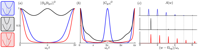
Figure 1: Comparison between three phonon configurations sketched on the left, from top to bottom: (i) Linear coupling ($\omega_{g}=\omega_{e},l\neq 0$), (ii) quadratic coupling ($\omega_{e}\neq\omega_{g},l=0)$, and (iii) both $(\omega_{e}\neq\omega_{g},l\neq 0)$. We show (a) the time evolution of $|\langle p_{g}|p_{g;t}\rangle|^{2}$ given in Eqs. (23, Two-level System coupled to Phonons: Full Analytical Solution) when the initial state is the ground-phonon vacuum, $p=0$; (b) the correlation function $|G_{g;t}|^{2}$ given in Eqs. (24, 34), for $\beta\hbar\omega_{e}=1$; and (c) the absorption spectrum $A(w)$ given in Eq. (35) for $T=0$, the delta functions being taken as Gaussians for representation purpose. (i) Blue curves: Linear coupling only ($\omega_{g}=\omega_{e}\equiv\omega$ and $1=\Lambda_{g}=\Lambda_{e}\equiv\Lambda$); (ii) black curves: Quadratic coupling only ($\omega_{e}=2\omega_{g}$ and $0=\Lambda_{g}=\Lambda_{e})$; (iii) red curves: Both couplings $(\omega_{e}=2\omega_{g}$ and $1=\Lambda_{g}=\Lambda_{e}/\sqrt{2})$.

Spatial shift and frequency change.— Ground- and excited-phonons prove even more useful for different phonon frequencies, $\omega_{g}\neq\omega_{e}$, that is, when the quadratic term is present in Eq. (Two-level System coupled to Phonons: Full Analytical Solution). In this case, it is still possible to find analytical expressions for the quantities considered in the linear limit, by using the same commutation procedure. To catch the consequences of different phonon frequencies, we here only give new expressions of some relevant quantities, with a few hints on how to obtain them. Detailed derivations will be given in an extended version. Some consequences of having a spatial shift, a frequency change or both are visualized in Fig. 1.

When $\omega_{e}\neq\omega_{g}$, that is, $\gamma_{{}_{-}}\neq 0$, the operator $b_{g}$ given in Eq. (9b) not only destroys but also creates an excited-phonon. Compared to Eq. (15), this leads to an increase of the number of ground-phonons in the excited-phonon vacuum,

$$\left\langle 0_{e}\right|b_{g}^{\dagger}b_{g}\left|0_{e}\right\rangle=\Lambda_{g}^{2}+\gamma_{{}_{-}}^{2},$$ (25)

This also transforms Eq. (17) into

$$b_{g}e^{-i\omega_{e}tb_{e}^{\dagger}b_{e}}=e^{-i\omega_{e}t(b_{e}^{\dagger}b_{e}+1)}\big{(}\tilde{D}^{\prime}_{t}b_{g}+\tilde{Q}^{\prime}_{t}b^{\dagger}_{g}{-}\tilde{\Lambda}^{\prime}_{t}\big{)},$$ (26)

with $\tilde{D}^{\prime}_{t}=\gamma_{{}_{+}}^{2}-\gamma_{{}_{-}}^{2}e^{2i\omega_{e}t}$, $\tilde{Q}^{\prime}_{t}=\gamma_{{}_{+}}\gamma_{{}_{-}}(1-e^{2i\omega_{e}t})$, and $\tilde{\Lambda}^{\prime}_{t}=\Lambda_{e}(\gamma_{{}_{+}}-\gamma_{{}_{-}}e^{2i\omega_{e}t})-\Lambda_{g}e^{i\omega_{e}t}$. The existence of two time-dependent terms, $e^{i\omega_{e}t}$ and $e^{2i\omega_{e}t}$, instead of $e^{i\omega t}$ only in the linear limit (see Eq.(18)), brings two oscillatory terms in the time evolution of the ground-phonon number, which now reads

$$\left\langle p_{g;t}\right|b_{g}^{\dagger}b_{g}\left|p_{g;t}\right\rangle=p|\tilde{D}^{\prime}_{t}|^{2}+(p+1)|\tilde{Q}^{\prime}_{t}|^{2}+|\tilde{\Lambda}^{\prime}_{t}|^{2}$$ (27)

$$=p{+}4\Lambda_{g}^{2}\sin^{2}\frac{\omega_{e}t}{2}{+}\frac{\omega_{e}^{2}{-}\omega_{g}^{2}}{\omega_{e}\omega_{g}}\Big{(}\Lambda_{e}^{2}{+}(2p{+}1)\frac{\omega_{e}^{2}{-}\omega_{g}^{2}}{4\omega_{e}\omega_{g}}\Big{)}\sin^{2}\omega_{e}t.$$

The quadratic coupling adds a faster oscillation to the time evolution of the ground-phonon number, with an amplitude that depends on the phonon number $p$. This faster oscillation, which disappears when $\omega_{e}=\omega_{g}$ in agreement with Eq. (19), still exists for zero spatial shift, $l=0$, that is, in the absence of linear coupling, $\Lambda_{e}=\Lambda_{g}=0$.

The correlation function for the spectral lineshapes requires the knowledge of $T_{p}$ defined in Eq. (21) with $\omega$ taken equal to $\omega_{e}$. The fact that the operator $b_{g}$ not only destroys but also creates an excited-phonon brings a recursion relation between four $T_{p}$’s, instead of three as in Eq.(22). For $T_{p}\equiv\tilde{D}_{t}^{{}^{\prime}p}\tilde{T}_{p}$, this recursion relation reads

$$0=a_{0}\,p\tilde{T}_{p}-\Big{(}(p-1)a_{1}+b_{1}\Big{)}\tilde{T}_{p-1}$$ (28)

$$\quad+\Big{(}(p-2)a_{2}+b_{2}\Big{)}\tilde{T}_{p-2}-\Big{(}(p-3)a_{3}+b_{3}\Big{)}\tilde{T}_{p-3}$$

for $p\geq 3$ while for $p=(1,2)$, it reduces to its first two and three terms, respectively. In the linear limit, this equation reduces to the difference of the recursion relations (22) for $T_{p}$ and $T_{p-1}$; so, we do recover the ‘linear-coupling’ result, but in a non-trivial way.

To solve the above recursion relation (28) beyond the linear limit, we introduce the generating function $\tilde{K}(x)=\sum_{p=0}^{\infty}x^{p}\tilde{T}_{p}$. It obeys a first-order differential equation

$$0{=}\Big{(}a_{0}{-}a_{1}x{+}a_{2}x^{2}{-}a_{3}x^{3}\Big{)}\frac{d\tilde{K}(x)}{dx}{+}\Big{(}-b_{1}{+}b_{2}x{-}b_{3}x^{2}\Big{)}\tilde{K}(x)\>$$ (29)

the solution of which reads, by using the explicit $(a_{i},b_{i})$ values, as

$$\tilde{K}(x)=\tilde{T}_{0}{\sqrt{\frac{1-\tilde{Q}^{2}_{t}}{(x{-}1)^{2}-\tilde{Q}_{t}^{2}}}}\exp\Big{(}\frac{-x\,\,\tilde{\Lambda}^{2}_{t}/\tilde{D}_{t}}{(x-1+\tilde{Q}_{t})(1-\tilde{Q}_{t})}\Big{)}{}\,\,\,$$ (30)

with $\tilde{Q}_{t}=e^{-i\omega_{e}t}\tilde{Q}^{\prime}_{t}$ and similarly for $(\tilde{D}_{t},\tilde{\Lambda}_{t})$.

To get $T_{p}$, we must extract the $x^{p}$ coefficient of $\tilde{K}(x)$. We do it by rewriting $\tilde{K}(x)$ as a product of two functions that are easy to expand in powers of $x$. After some algebra, we end with

$$\langle p_{g}|p_{g;t}\rangle = \tilde{T}_{0}\>e^{-i\omega_{e}t/2}\left(\frac{\tilde{D}_{t}}{1+\tilde{Q}_{t}}\right)^{p}$$

$$\times \sum_{k=0}^{p}\left(\frac{1+\tilde{Q}_{t}}{1-\tilde{Q}_{t}}\right)^{k}L^{-\frac{1}{2}}_{p-k}(0)L^{-\frac{1}{2}}_{k}\Big{(}\frac{-\tilde{\Lambda}^{2}_{t}}{\tilde{D}_{t}(1-\tilde{Q}_{t})}\Big{)}$$

with $\tilde{T}_{0}$ given by

$$\tilde{T}_{0}=(\gamma_{{}_{+}}^{2}-\gamma_{{}_{-}}^{2}e^{-2i\omega_{e}t})^{-1/2}\exp({-\Lambda_{g}\Lambda_{e}\dfrac{1-e^{-i\omega_{e}t}}{\gamma_{{}_{+}}-\gamma_{{}_{-}}e^{-i\omega_{e}t}}}).$$ (32)

This result reduces to Eq. (23) in the linear limit: Indeed, $\tilde{Q}_{t}=0$ and $-\tilde{\Lambda}^{2}_{t}/\tilde{D}_{t}=|\Lambda_{t}|^{2}$ while the sum in Eq. (Two-level System coupled to Phonons: Full Analytical Solution) follows from the addition formula of Laguerre polynomials Abramowitz and Stegun (1964), i.e., $\sum_{k=0}^{p}L^{-\frac{1}{2}}_{p-k}(0)L_{p}^{-\frac{1}{2}}(|\Lambda_{t}|^{2})=L_{p}(|\Lambda_{t}|^{2}).$

Consequences of spatial shift and frequency change.— Figure 1a shows $|\langle p_{g}|p_{g;t}\rangle|^{2}$ for the three relevant coupling configurations, namely, a spatial shift $l\neq 0$, a frequency change $\omega_{g}\neq\omega_{e}$ and both, when the initial state is the ground-phonon vacuum. We see that the likelihood that the phonon number state remains in the initial state is much smaller when $l\neq 0$ than when $l=0$, that is, when the linear coupling vanishes. Mathematically, this is due to the fact that when $\Lambda_{e}=\Lambda_{g}=0$, the exponential factor in $\tilde{T}_{0}$ reduces to 1. We also find that, for finite $\Lambda_{g,e}$’s, the likelihood for the phonon state to remain in its initial state is smaller when $\omega_{g}\neq\omega_{e}$ than when $\omega_{g}=\omega_{e}$, that is, when the quadratic coupling vanishes. These observations are born out by the changing distribution of the absorption spectra, shown in Fig. 1c.

With $\langle p_{g}|p_{g;t}\rangle$ known, it becomes possible to derive the correlation function for the absorption lineshape when the phonon bath is at thermal equilibrium, as defined in Eq. (20) with $\omega$ taken as $\omega_{g}$. It reads

$$G_{g;t}=\frac{1}{Z_{g}}e^{-i\Omega_{eg}t}e^{i(\omega_{g}{-}\omega_{e})\frac{t}{2}}\sum_{p=0}^{\infty}(e^{-\beta\hbar\omega_{g}+i\omega_{g}t}\tilde{D}_{t})^{p}\tilde{T}_{p},\quad\>\>$$ (33)

where $Z_{g}$ is the partition function calculated with $\omega_{g}$. This quantity can be conveniently written in terms of the generating function $\tilde{K}(x)$ given in Eq. (30), as

$$G_{g;t}=\frac{1}{Z_{g}}e^{-i\Omega_{eg}t}e^{i(\omega_{g}-\omega_{e})t/2}$$ (34)

$$\hskip 50.00008pt\times\tilde{K}\Big{(}e^{-\beta\hbar\omega_{g}}(\gamma_{{}_{+}}^{2}e^{i(\omega_{g}-\omega_{e})t}-\gamma_{{}_{-}}^{2}e^{i(\omega_{g}+\omega_{e})t})\Big{)}.$$

For $\gamma_{{}_{-}}=0$, it reduces to the linear limit, Eq. (24), while for zero temperature, $G_{g;t}$ reduces to $e^{-i\Omega_{eg}t}e^{i(\omega_{g}-\omega_{e})t/2}\tilde{T}_{0}$. By writing $\tilde{T}_{0}$ in terms of Hermite polynomials ${\rm H}_{n}(x)$ through the Mehler’s formula, we can get the absorption spectrum at $T=0$ as illustrated in Fig. 1c and given by

$$A(w)\!\! = \!\!\frac{2\pi}{\gamma_{+}}e^{-\frac{\Lambda_{e}\Lambda_{g}}{\gamma_{+}}}\sum_{n=0}^{\infty}\frac{1}{n!}\!\left(-\frac{\gamma_{-}}{2\gamma_{+}}\right)^{n}\left({\rm H}_{n}\Big{(}\frac{\Lambda_{g}}{\sqrt{-2\gamma_{+}\gamma_{-}}}\Big{)}\right)^{2}$$ (35)

$$\hskip 28.45274pt\times\delta\big{(}w-\Omega_{eg}-\frac{\omega_{e}-\omega_{g}}{2}-n\omega_{e}\big{)}.$$

The above results (34,35), together with Eqs. (Two-level System coupled to Phonons: Full Analytical Solution,32), are the first analytical expressions that include both ‘linear’ and quadratic couplings for a two-level system coupled to phonons. The correlation function $G_{g;t}$ is shown in Fig. 1b: Compared to the overlap $\langle p_{g}|p_{g;t}\rangle$, a change in periodicity occurs when $\omega_{g}\not=\omega_{e}$, due to the additional oscillatory terms $e^{i(\omega_{g}-\omega_{e})t}$ and $e^{i(\omega_{g}+\omega_{e})t}$ appearing in Eq. (34). Difference in the phonon frequencies also modifies the position and amplitude of the energy poles in the absorption spectrum. Even at $T=0$, the zero-point-energy difference shifts the spectrum compared to linear coupling (see Fig. 1c). Increasing the temperature will add more energy poles to the spectrum as more ground-phonon Fock states come into play.

In conclusion, we propose a conceptually different approach to the independent boson model. It relies on a diagonal representation using two sets of phonons physically relevant for the problem, namely, ground-phonons and excited-phonons that depend on the level occupied by the electronic system. By capturing the essence of the problem, this representation removes couplings in a natural way from the very first line, without the need of any transformation. It considerably simplifies the resolution of the problem, by solely relying on commutation relations between the two types of phonon operators. Besides recovering the known results in a simple way, we are able to go further in the model complexity by solving the problem for different phonon frequencies, that is, quadratic coupling, and to study its intricate consequences on the time dependence of the correlation functions for all coupling configurations. While the independent boson model is the simplest model to study electron-phonon interactions, we anticipate that the physical approach presented here can allow for simpler resolutions of more complex problems, starting with the spin-boson model.

References

• Breuer and Petruccione (2007) H.-P. Breuer and F. Petruccione, The Theory of Open Quantum Systems (Oxford University Press, 2007).
• Weiss (2012) U. Weiss, Quantum dissipative systems, Vol. 13 (World scientific, 2012).
• May and Kühn (2001) V. May and O. Kühn, Charge and Energy Transfer Dynamics in Molecular Systems (Wiley-VCH, Berlin, 2001).
• Valkunas et al. (2013) L. Valkunas, D. Abramavičius,  and T. Mančal, Molecular Excitation Dynamics and Relaxation: Quantum Theory and Spectroscopy (Wiley-VCH, Weinheim, 2013).
• Ferry and Goodnick (1997) D. Ferry and S. M. Goodnick, Transport in nanostructures (Cambridge university press, 1997).
• Wiseman and Milburn (2009) H. M. Wiseman and G. J. Milburn, Quantum measurement and control (Cambridge university press, 2009).
• Schlosshauer (2007) M. Schlosshauer, Decoherence and the Quantum-to-Classical Transition (Springer, Berlin, 2007).
• Leggett et al. (1987) A. J. Leggett et al.Rev. Mod. Phys. 59, 1 (1987).
• Mahan (2000) G. D. Mahan, Many-Particle Physics, 3rd ed. (Kluwer Academic Publishers, 2000) Chps. 1 and 4.
• Cai et al. (1989) W. Cai, T. F. Zheng, P. Hu, B. Yudanin,  and M. Lax, Phys. Rev. Lett. 63, 418 (1989).
• Morillo and Cukier (1996) M. Morillo and R. I. Cukier, Phys. Rev. B 54, 13962 (1996).
• Vagov et al. (2002) A. Vagov, V. M. Axt,  and T. Kuhn, Phys. Rev. B 66, 165312 (2002).
• Hohenester and Stadler (2004) U. Hohenester and G. Stadler, Phys. Rev. Lett. 92, 196801 (2004).
• Jirari and P tz (2007) H. Jirari and W. P tz, EPL (Europhysics Letters) 77, 50005 (2007).
• Duke and Mahan (1965) C. B. Duke and G. D. Mahan, Phys. Rev. 139, A1965 (1965).
• Steinbach et al. (1999) D. Steinbach, G. Kocherscheidt, M. U. Wehner, H. Kalt, M. Wegener, K. Ohkawa, D. Hommel,  and V. M. Axt, Phys. Rev. B 60, 12079 (1999).
• Castella and Zimmermann (1999) H. Castella and R. Zimmermann, Phys. Rev. B 59, R7801 (1999).
• Axt et al. (1999) V. Axt, M. Herbst,  and T. Kuhn, Superlattices and Microstr. 26, 117 (1999).
• Krummheuer et al. (2002) B. Krummheuer, V. M. Axt,  and T. Kuhn, Phys. Rev. B 65, 195313 (2002).
• Besombes et al. (2001) L. Besombes, K. Kheng, L. Marsal,  and H. Mariette, Phys. Rev. B 63, 155307 (2001).
• Scully and Zubairy (1997) M. O. Scully and M. S. Zubairy, Quantum optics (Cambridge university press, 1997).
• Loudon (2000) R. Loudon, The Quantum Theory of Light, 3rd ed. (Oxford University Press, Oxford, 2000).
• Silbey and Munn (1980) R. Silbey and R. W. Munn, J. Chem. Phys. 72, 2763 (1980).
• Mukamel (1995) S. Mukamel, Principles of nonlinear spectroscopy (Oxford University Press, Oxford, 1995) Ch. 8.
• Nitzan (2006) A. Nitzan, Chemical dynamics in condensed phases: Relaxation, transfer and reactions in condensed molecular systems (Oxford university press, 2006).
• Munn and Siebrand (1970) R. W. Munn and W. Siebrand, J. Chem. Phys. 52, 47 (1970).
• Coropceanu et al. (2007) V. Coropceanu, J. Cornil, D. A. da Silva Filho, Y. Olivier, R. Silbey,  and J.-L. Brédas, Chem. Rev. 107, 926 (2007), and references therein.
• Sluch et al. (2001) M. I. Sluch, A. Godt, U. H. Bunz,  and M. A. Berg, J. Am. Chem. Soc. 123, 6447 (2001).
• Coropceanu et al. (2002) V. Coropceanu, M. Malagoli, D. da Silva Filho, N. Gruhn, T. Bill,  and J. Brédas, Phys. Rev. Lett. 89, 275503 (2002).
• Liu et al. (2007) L. T. Liu, D. Yaron,  and M. A. Berg, J. Phys. Chem. C 111, 5770 (2007).
• Uskov et al. (2000) A. V. Uskov, A.-P. Jauho, B. Tromborg, J. Mørk,  and R. Lang, Phys. Rev. Lett. 85, 1516 (2000).
• Muljarov and Zimmermann (2004) E. A. Muljarov and R. Zimmermann, Phys. Rev. Lett. 93, 237401 (2004).
• McCumber and Sturge (1963) D. McCumber and M. Sturge, J. Appl. Phys. 34, 1682 (1963).
• Krivoglaz (1964) M. Krivoglaz, Fiz. Tverd. Tela 6, 1707 (1964).
• Jones and Zewail (1978) K. Jones and A. Zewail, Springer Series in Chemical Physics, Springer, Berlin, Heidelberg New York 3, 196 (1978).
• Di Bartolo (2010) B. Di Bartolo, Optical interactions in solids (World Scientific Publishing Company, 2010).
• Levenson (1971) G. Levenson, physica status solidi (b) 43, 739 (1971).
• Osad’ko (1973) I. Osad’ko, Sov. Phys. Solid State 14, 2522 (1973).
• Goupalov et al. (2002) S. Goupalov, R. Suris, P. Lavallard,  and D. Citrin, IEEE J. S. Top. Quantum Electron. 8, 1009 (2002).
• Hsu and Skinner (1984) D. Hsu and J. Skinner, J. Chem. Phys. 81, 1604 (1984).
• Hizhnyakov et al. (2002) V. Hizhnyakov, H. Kaasik,  and I. Sildos, Phys. Status Solidi B 234, 644 (2002).
• Huang and Rhys (1950) K. Huang and A. Rhys, Proc. R. Soc. Lond. A 204, 406 (1950).
• Abramowitz and Stegun (1964) M. Abramowitz and I. A. Stegun, Handbook of mathematical functions: With formulas, graphs, and mathematical tables, Vol. 55 (Courier Corporation, 1964) eq. (22.12.6), p. 785.