A new parton model for the soft interactions at high energies.

Abstract

We propose a new parton model and demonstrate that the model describes the relevant experimental data at high energies. The model is based on Pomeron calculus in 1+1 space-time dimensions, as suggested in Ref. KLL , and on simple assumptions regarding the hadron structure, related to the impact parameter dependence of the scattering amplitude. This parton model evolves from QCD, assuming that the unknown non-perturbative corrections lead to fixing the size of the interacting dipoles. The advantage of this approach is that it satisfies both t-channel and s-channel unitarity, and can be used for summing all diagrams of Pomeron interactions, including Pomeron loops. We can use this approach for all reactions: dilute-dilute (hadron-hadron), dilute- dense (hadron - nucleus) and dense-dense (nucleus-nucleus) for the scattering of parton systems. Unfortunately, we are still far from being able to tackle this problem in the effective QCD theory at high energy (i.e. in the CGC /saturation approach).

I Introduction

In our previous papers GLP1 ; GLP2 ; GLMNI ; GLM2CH ; GLMINCL ; GLMCOR ; GLMSP ; GLMACOR we demonstrated that it is possible to build a model, based on the effective QCD theory at high energies: i.e. Colour Glass Condensate (CGC) approach (see Ref.KOLEB for the review). The success of the model emanates from two principle ideas, which are supported by experimental data: (i) typical distances in the soft processes at high energies, turn out to be rather short; and (ii) the CGC approach can be re-written in an equivalent form, as the interaction of BFKL PomeronsAKLL in a limited range of rapidities ( $Y\leq Y_{\rm max}$):

$$Y\,\leq\,\frac{2}{\Delta_{\mbox{\tiny BFKL}}}\,\ln\left(\frac{1}{\Delta^{2}_{\mbox{\tiny BFKL}}}\right)$$ (1)

where $\Delta_{\mbox{\tiny BFKL}}$ denotes the intercept of the BFKL PomeronBFKL . In our model $\Delta_{\mbox{\tiny BFKL}}\,\approx\,0.2-0.25$ leading to $Y_{max}=20-30$, which covers all collider energies.

The equivalence between the CGC approach and the BFKL Pomeron calculus is very important, since (i) it shows that the CGC approach satisfies t-channel unitarity, which is a prerequisite for any effective theory at high energies and (ii) it allows us to consider elastic and diffraction processes, and processes of multiparticle generation, on the same footing. The last statement follows from the AGK cutting rulesAGK , which has been proven for inclusive productionKOTU , but not for correlations KOJA .

In Ref.AKLL it was shown than in the rapidity range of Eq. (1) we can use the MPSI approximationMPSI , which sums the large Pomeron loops for the following Hamiltonian

$${\cal H} = \frac{N_{c}^{2}}{2\pi\bar{\alpha}_{s}}\int\bar{P}(x,y)\nabla^{2}_{x}\nabla^{2}_{y}\left[K(x,y|z)P(x,z)+P(z,y)-P(x,y)-P(x,z)P(z,y)\right]$$ (2)

$$-P(x,y)\nabla^{2}_{x}\nabla^{2}_{y}\left[K(x,y|z)\bar{P}(x,z)\bar{P}(z,y)\right]$$

where

$$K(x,y|z)=\frac{(\boldsymbol{x}-\boldsymbol{y})^{2}}{(\boldsymbol{x}-\boldsymbol{z})^{2}(\boldsymbol{y}-\boldsymbol{z})^{2}},$$

$P$ and $\bar{P}$ denote the BFKL Pomeron fields.

The commutation relations are of the form

$$[\bar{P}(x,y),P(u,v)]\,=\,\gamma(x,y;u,v)$$ (3)

where $\gamma(x,y;u,v)$ is the scattering amplitude of a dipole $(x,y)$ on the dipole $(u,v)$

$$\gamma(x,y;u,v)=\frac{\alpha_{s}^{2}}{32\pi^{2}}\ln^{2}\frac{(\boldsymbol{x}-\boldsymbol{u})^{2}(\boldsymbol{y}-\boldsymbol{v})^{2}}{(\boldsymbol{x}-\boldsymbol{v})^{2}(\boldsymbol{y}-\boldsymbol{u})^{2}}$$ (4)

The above form of the Hamiltonian was suggested in Ref.BRAUN as the natural way for summing all BFKL Pomeron diagrams with only triple Pomeron interactions. Below, we will denote this Hamiltonian by ${\cal H}_{\rm B}$.

In Ref.KLL it is shown that the Hamiltonian of Eq. (2) cannot be the correct one, since it violates s-channel unitarity. In other words, we can use ${\cal H}_{\rm B}$ only for summing the large Pomeron loops in the MPSI approximation, but cannot use it for a general description of the high energy interaction in QCD, nor even for the description of the DIS, which is given by Balitsky - Kovchegov equationBK , and was considered to be the most reliable equation in the framework of the CGC approach. It should be stressed, that in the CGC approach, we do not have a general Hamiltonian that describes the interaction of two dense, or of two dilute systems of partons, although some work in this direction has been doneFOAM . Unfortunately, no progress in formulating the BFKL Pomeron calculus for these systems has been achieved in Ref.KLL .

However, in Ref.KLL such a Hamiltonian is constructed for the 1+1 Reggeon Field Theory, which corresponds to QCD in which the size of the interacting dipoles is fixedMUDI ; LELU . In this model the BFKL equation for the dipole scattering cross section $\sigma$ at a rapidity $Y$ is reduced to

$$\frac{d\sigma\left(Y\right)}{dY}\,\,=\,\,\Delta\,\sigma\left(Y\right),$$ (5)

where $\Delta$ denotes the BFKL intercept. The Eq. (5) reproduces the power-like increase of the cross section with energy, $\exp(\Delta Y)=(1/x)^{\Delta}$. For the scattering amplitude $N$ we obtain the non-linear equation:

$$\frac{dN\left(Y\right)}{dY}\,\,=\,\,\Delta\,\Bigg{(}N\left(Y\right)\,\,-\,\,N^{2}\left(Y\right)\Bigg{)}$$ (6)

this form is similar to that of the Balitsky-Kovchegov non-linear equationBK . Note that Eq. (6) does not depend on the impact parameter . This fact is also in agreement with the BFKL approach, in which the average momentum of the produced colourless dipoles increases with energy since $p_{T}\propto\,s^{\lambda}$, and Gribov diffusionGRIBDIF in impact parameter with $\Delta b\propto\frac{1}{p_{T}}n\,=\,\frac{1}{p_{T}}\Delta Y$, leads to $\Delta b\to 0$ at high energies. We can consider this simple model as the QCD approach in which the typical size of the colourless dipoles are fixed, and do not depend on energy. In other words, we can view this simple approach as a new parton model for the high energy interactionPARTMOD .

In this model we encountered the same problems with $s$-channel unitarity as in QCD at high energy, however we have identified the Pomeron Hamiltonian which cures all these problemsKLL . In the next section we will briefly review our finding. In section 3 we propose a model based on this Hamiltonian, while in section 4 we compare the predictions of this model with the relevant experimental data. We summarize our results in the Conclusions.

II A new parton model

Below we give a short review of sections 4 and 5 of Ref.KLL , where 1+1 Reggeon Field Theory(RFT) is discussed. We emphasis section 5, which contains the results that we are going to use in building our model.

II.1 Violation of the s-channel unitarity in 1 + 1 RFT

As a direct generalization of the original QCD to 1+1 RFT, the scattering matrix of the projectile consisting of $m$ dipoles on a target consisting of $\bar{n}$ dipoles, is given as by

$$\langle m|\bar{n}\rangle=\int d\bar{P}\delta(\bar{P})(1-P)^{m}(1-\bar{P})^{\bar{n}}$$ (7)

The evolution in rapidity takes the form

$$\langle m|\bar{n}\rangle_{Y}=\int d\bar{P}\delta(\bar{P})(1-P)^{m}e^{HY}(1-\bar{P})^{\bar{n}}$$ (8)

The 1+1 analog of the BK evolution (see Eq. (6)) is given by the Hamltonian

$${\cal H}_{\rm BK}=-\frac{1}{\gamma}\Big{(}\bar{P}P-\bar{P}P^{2}\Big{)}$$ (9)

As previously, we take $P$ and $\bar{P}$ to satisfy the dilute limit algebra with the commutator Eq. (3), such that

$$P\,=\,-\gamma\frac{d}{d\bar{P}};\ \ \ \ \ \gamma\,\sim\,\bar{\alpha}_{S}^{2}>0~{}~{}~{}~{}\leftarrow~{}~{}~{}\mbox{{Eq.~{}(\ref{DDAM})} in 1+1 RFT}$$ (10)

To comprehend the origin of $s$-channel unitarity, we consider the infinitesimal evolution ($\delta Y$) of the projectile and target wave functions with the Hamiltonian ${\cal H}_{\rm BK}$:

$$\langle m|e^{{\cal H}_{\rm BK}\delta Y}\,\,\propto\,\,(1\,\,-\,\,m\,\delta Y)\langle m|\,\,+\,\,m\,\delta Y\,\langle m+1|$$ (11)

$$e^{{\cal H}_{\rm BK}\,\delta Y}|\bar{n}\rangle=(1\,+\,\bar{n}\,\delta Y)|\bar{n}\rangle\,\,-\,\,\bar{n}[1+\gamma(\bar{n}-1)]\,\delta Y|\bar{n}-1\rangle\,\,+\,\,\gamma\bar{n}(\bar{n}-1)\,\delta Y|\bar{n}-2\rangle$$ (12)

Note the difference between these two equations. The coefficient in front of an $n$-dipole state has the meaning of, the probability to find this number of dipoles in the wave function. The projectile evolution, given by Eq. (11) is unitary: all the probabilities in the evolved state remain positive and smaller than unity, and the sum of the probabilities add up to unity.

On the other hand, the target evolution is non-unitary. Indeed, we face two difficulties with the unitarity: (i) the probability to find the initial state $|\bar{n}\rangle$ after a short interval of evolution exceeds unity; and (ii) the probability to find a state $|\bar{n}-1\rangle$ is negative. The coefficients still sum to unity as for the projectile, but clearly the target evolution violates unitarity.

The Braun Hamiltonian of Eq. (2) takes the following form in 1+1 RFT:

$${\cal H}_{\rm B}\,\,=\,\,-\frac{1}{\gamma}\left[\bar{P}P-\bar{P}P^{2}-\bar{P}^{2}P\right]$$ (13)

Exploring the same question about $s$-channel unitarity as in Eq. (11) and Eq. (12) we obtain for the evolution of the target wave function:

$$e^{{\cal H}_{\rm B}\,\delta Y}|\bar{n}\rangle\,\,\approx\,\,(1+{\cal H}_{\rm B}\delta Y)|\bar{n}\rangle\,\,=\,\,(1-\bar{n}\delta Y)|\bar{n}\rangle+\bar{n}\,\delta Y|\bar{n}+1\rangle-\gamma\bar{n}(\bar{n}-1)\delta Y|\bar{n}-1\rangle+\gamma\bar{n}(\bar{n}-1)\delta Y|\bar{n}-2\rangle$$ (14)

One can see that Eq. (14) violates unitarity, but this violation is smaller than in Eq. (12), being $O(\gamma)$, and it is small for small $\bar{n}$ . However, the coefficient of the term $|\bar{n}\rangle$ is still negative, and becomes large parametrically, long before the saturation limit is reached. Since Eq. (13) is symmetric between the target and the projectile, the projectile evolution now is also non-unitary, and involves negative probabilities. The fact that the violation of the unitarity occurs at large $\bar{n}$ suggets that one reconsiders the commutation relations of Eq. (3) and Eq. (10), which we discuss in the next subsection.

II.2 Commutators

Using the commutators of Eq. (3) and Eq. (10), the scattering matrix can be calculated explicitly (for $m+1<\bar{n}$)

$$\langle m|\bar{n}\rangle\,=\,\sum_{l=0}^{m}\frac{m!\bar{n}!}{(m-l)!\,(\bar{n}-l)!\,l!}(-\gamma)^{l}$$ (15)

In particular

$$\langle 1|\bar{n}\rangle=1-\bar{n}\gamma$$ (16)

From the above one can see that the amplitudes become negative for $\bar{n}\,>\,1/\gamma$, and when a single dipole of the projectile scatters on several dipoles of the target, our commutation relation does not allow us to account for multiple scattering corrections.

Therefore, as well as curing the problems with unitarity, we need to change Eq. (3)(Eq. (10)) in a such way that the scattering matrix will have the form:

$$\langle 1|\bar{n}\rangle=\sum_{k=0}^{\bar{n}}\frac{\bar{n}!}{(\bar{n}-k)!k!}(-\gamma)^{k}$$ (17)

so as to correctly account for multiple rescatterings.

In Ref.KLL the following commutator which reproduce Eq. (17) is proposed.

$$\Big{(}1\,\,-\,\,P\Big{)}\Big{(}1\,\,-\,\,\bar{P}\Big{)}\,\,=\,\,(1-\gamma)\Big{(}1\,\,-\,\,\bar{P}\Big{)}\Big{(}1\,\,-\,\,P\Big{)}$$ (18)

Eq. (18) gives the correct factor $(1-\gamma)^{\bar{n}}$ that includes all multiple scattering corrections, while all the dipoles remain intact, and can subsequently scatter on additional projectile or target dipoles. For small $\gamma$, and in the regime where $P$ and $\bar{P}$ are also small, we obtain

$$[P,\bar{P}]=-\gamma+...$$ (19)

consistent with our original expression.

Note, that the algebra of Eq. (18) is equivalent to the following representation

$$1-\bar{P}=e^{-\ln(1-\gamma)\frac{d}{d\Phi}},;\ \ \ \ \ \ 1-P=e^{-\Phi}$$ (20)

where $\Phi$ and $\bar{\Phi}$ have the same meaning as in Eq. (2).

In the calculation of an amplitude of the type of Eq. (17), once all the factors of $1-\bar{P}$ are commuted through to the left, then in the remaining matrix element $\bar{P}$ operates on the $\delta$-function and thus vanishes. The remaining factors of $(1-P)$ also become unity, since a factor of $\Phi$ is equivalent to a derivative acting on the $\delta$-function, and vanishes when integrated over $\bar{P}$.

With the new algebra we have

$$\langle m|\bar{n}\rangle=(1-\gamma)^{m\bar{n}}$$ (21)

which is a simple and intuitive result: the S-matrix of dipole-dipole scattering raised to the power of the number of dipole pairs that scatter.

It should be stressed, that the modification of the Pomeron algebra is not a matter of choice, but is necessary to obtain the amplitude of Eq. (17), which is unitary for arbitrary numbers of colliding dipoles. However, the question of the unitarity of the evolution is a completely separate one. We will examine the s-channel unitarity for the Braun Hamiltonian, since we plan to use this Hamiltonian for the description of hadron-hadron scattering at high energy.

We write the Braun Hamiltonian in a more convenient form:

$${\cal H}_{\rm B}\,\,=\,\,-\frac{1}{\gamma}\Big{[}(1-\bar{P})P-(1-\bar{P})^{2}P+(1-\bar{P})P^{2}-P^{2}\Big{]}$$ (22)

The action on the projectile and the target is obviously symmetric, as the Hamiltonian is self dual under the transformation $P\rightarrow\bar{P}$.

$$e^{{\cal H}_{\rm B}\,\delta Y}|\bar{n}\rangle=\left[1+\frac{\delta Y}{\gamma}\left[1-(1-\gamma)^{\bar{n}}\right]^{2}\right]|\bar{n}\rangle-\frac{\delta Y}{\gamma}\left[1-(1-\gamma)^{\bar{n}}\right]\left[2-(1-\gamma)^{\bar{n}}\right]|\bar{n}+1\rangle+\frac{\delta Y}{\gamma}\left[1-(1-\gamma)^{\bar{n}}\right]|\bar{n}+2\rangle$$ (23)

$$\langle m|e^{{\cal H}_{\rm B}\,\delta Y}=\left[1+\frac{\delta Y}{\gamma}\left[1-(1-\gamma)^{m}\right]^{2}\right]\langle m|-\frac{\delta Y}{\gamma}\left[1-(1-\gamma)^{m}\right]\left[2-(1-\gamma)^{m}\right]\langle m+1|+\frac{\delta Y}{\gamma}\left[1-(1-\gamma)^{m}\right]\langle m+2|$$ (24)

This result is a disaster: the evolution of both, projectile and target are non-unitary. In fact the lack of unitarity occurs for an arbitrary number of dipoles $m$ and $\bar{n}$. It is shown in Ref.KLL that the terms that include the four Pomeron interaction, do not help.

II.3 The Hamiltonian of the new parton model

In Ref.KLL a new Hamiltonian is proposed

$${\cal H}_{\rm NPM}=-\frac{1}{\gamma}\bar{P}P$$ (25)

where NPM stands for “new parton model”. The fact that it is self dual is obvious. In the limit of small $\bar{P}$ this Hamiltonian reproduces ${\cal H}_{\rm BK}$ ( see Ref.KLL for details). This condition is important for fixing the form of ${\cal H}_{\rm NPM}$.

To check unitarity we consider:

$$e^{{\cal H}_{\rm NPM}\,\delta Y}|\bar{n}\rangle=\left[1-\frac{\delta Y}{\gamma}[1-(1-\gamma)^{\bar{n}}]\right]|\bar{n}\rangle+\frac{\delta Y}{\gamma}[1-(1-\gamma)^{\bar{n}}]|\bar{n}+1\rangle$$ (26)

Performing the operation in Eq. (26), we first express the $P^{\dagger}$ in terms of $\bar{P}$. To do this, recall that $P^{\dagger}$ should annihilate a dipole when acting on the wave function. Using eq.(20) we can write

$$P^{\dagger}=\frac{d}{d\Phi}e^{\Phi}=\frac{1}{\gamma}\ln(1-\bar{P})\frac{1}{1-P};\ \ \ \ \ \ \bar{P}^{\dagger}=-\frac{1}{\gamma}e^{-\gamma\frac{d}{d\Phi}}\Phi=\frac{1}{\gamma}\frac{1}{1-\bar{P}}\ln(1-P)$$ (27)

For simplicity, in the above equations we have used $\ln(1-\gamma)\approx-\gamma$, since $\gamma\sim\alpha_{s}^{2}\ll 1$

To check for unitarity, we see that

$$e^{{\cal H}_{\rm NPM}\,\,\delta Y}|\bar{n}\rangle=\left[1-\frac{\delta Y}{\gamma}[1-(1-\gamma)^{\bar{n}}]\right]|\bar{n}\rangle+\frac{\delta Y}{\gamma}[1-(1-\gamma)^{\bar{n}}]|\bar{n}+1\rangle$$ (28)

showing that this evolution is clearly unitary. Due to self duality, it is clear that the evolution of the projectile wave function is unitary as well.

It is interesting that Eq. (28) displays saturation behavior very similar to that expected from QCD evolution, namely at large $\bar{n}$, the change in the wave function is independent of the number of dipoles $\bar{n}$. In the BK approach in QCD, the wave function never saturates(see Eq. (11)), and saturation of the scattering amplitudes is due to multiple scattering effects.

II.4 Equations of motion and the scattering amplitude

The general form of the equation of motion follows from

$$\frac{dP}{d\eta}\,=\,\Big{[}{\cal H},P\Big{]}\,;~{}~{}~{}~{}{\rm and}~{}~{}~{}~{}\frac{d\bar{P}}{d\eta}\,=\,\Big{[}{\cal H},\bar{P}\Big{]}$$ (29)

For the Hamiltonian ${\cal H}_{\rm NPM}$ we get

$$\frac{dP}{d\eta}\,=\,\left(1-\bar{P}\right)\,\left(1-P\right)\,P;~{}~{}~{}~{}~{}~{}~{}\frac{d\bar{P}}{d\eta}\,=\,-\left(1-P\right)\,\left(1-\bar{P}\right)\,\bar{P};$$ (30)

Interestingly, although it is not obvious from the form of the Hamiltonian (see Eq.(22)), the evolution has the same fixed points as in two transverse dimensions, $(0,0),\ (1,0),\ (0,1),\ (1,1)$.

Since the Hamiltonian is conserved, we have

$$\bar{P}P={\rm Const}\equiv{\rm\alpha}$$ (31)

Using this conservation relation we obtain the following equations of motion:

$$\frac{dP}{d\eta}\,=\,\left(P\,-\,\alpha\right)\,\left(1-P\right);\ \ \ \ \ \ \frac{d\bar{P}}{d\eta}\,=-\,\left(\bar{P}\,-\,\alpha\right)\,\left(1-\bar{P}\right)$$ (32)

It is instructive to note that fixed points $(0,0),\ (0,1)$ and $(1,0)$ are not present in these equations, which means that they are not reachable at $\alpha\neq 0$. The point $(1,1)$ is also not reachable by evolution for $\alpha\neq 1$. Eq. (32) has only two interesting fixed points: $\left(1,\alpha\right)$ and $\left(\alpha,1\right)$. Since for any physical initial condition $P(0)>\alpha$, the asymptotics at $\eta\rightarrow\infty$ is always dominated by the fixed point $(P=1,\bar{P}=\alpha)$, while for $\eta\rightarrow 0$ the point $(P=\alpha,\bar{P}=1)$ is approached.

The general solution to Eq. (30) takes the form:

$$P(\eta)\,=\,\frac{\alpha+\beta e^{(1-\alpha)\eta}}{1+\beta e^{(1-\alpha)\eta}};\ \ \ \ \bar{P}(\eta)=\frac{\alpha(1+\beta e^{(1-\alpha)\eta})}{\alpha+\beta e^{(1-\alpha)\eta}};$$ (33)

where the parameters $\beta$ and $\alpha$ should be determined from the boundary conditions:

$$P(\eta=0)\,=\,p_{0};\,\,\,\,\,\,\,\,\bar{P}(\eta=Y)\,=\,\frac{\alpha}{P(\eta=Y)}\,=\,\bar{p}_{0}$$ (34)

One can see that for $p_{0}\,>\,\bar{p}_{0}$ and $e^{(1-\alpha)Y}\,\gg\,1$ Eq. (34) leads to

$$\beta\,=\,\frac{p_{0}\,-\,\alpha}{1\,-\,p_{0}}\,=\,\frac{p_{0}\,-\,\bar{p}_{0}}{1-p_{0}};\,\,\,\,\,\,\,\,\,\,\alpha\,=\,\bar{p}_{0};$$ (35)

For a symmetric boundary condition $p_{0}=\bar{p}_{0}$, Eq. (34) gives $P(0)=\bar{P}(Y)$, and the solution takes the form

$$P(\eta) = \frac{\alpha+\sqrt{\alpha}e^{(1-\alpha)(\eta-Y/2)}}{1+\sqrt{\alpha}e^{(1-\alpha)(\eta-Y/2)}}$$ (36)

$$\bar{P}(\eta) = \frac{\alpha\left(1+\sqrt{\alpha}e^{(1-\alpha)(\eta-Y/2)}\right)}{\alpha+\sqrt{\alpha}e^{(1-\alpha)(\eta-Y/2)}}$$

$$P(\eta) = \bar{P}(Y-\eta)$$

This solution has a distinct BFKL limit. Indeed, for $\alpha\ll 1$ and $e^{-Y/2}=a\sqrt{\alpha}$ with $1/\alpha\gg a\gg 1$.

We now have the BFKL-like contribution

$$P(\eta)\,\,\approx\,\,a\alpha e^{\eta}$$ (37)

Comparing Eq. (37) with Eq. (5) and Eq. (6) one can see that the variable $Y$ in all our formulae is actually equal to $\Delta Y$. The exponential “BFKL-like” growth continues until the Pomeron reaches the value $P(Y)=1$.

The classical solutions determine the scattering amplitude in the classical approximation. The scattering amplitude has a path integral representation. The Pomeron Lagrangian that generates the equations of motion eq.(30) is

$${\cal L}^{\rm NPM}=\int_{0}^{Y}d\eta\left[\frac{1}{\gamma}\ln(1-P)\frac{\partial}{\partial\eta}\ln(1-\bar{P})-H\right]=\frac{1}{\gamma}\int_{0}^{Y}d\eta\left[\ln(1-P)\frac{\partial}{\partial\eta}\ln(1-\bar{P})+\bar{P}P\right]$$ (38)

The scattering amplitude is then given by

$$S^{\rm NPM}_{m\bar{n}}(Y)=\int dP(\eta)d\bar{P}(\eta)e^{\frac{1}{\gamma}\int_{0}^{Y}d\eta\left[\ln(1-P)\frac{\partial}{\partial\eta}\ln(1-\bar{P})+\bar{P}P\right]}(1-P(Y))^{m}(1-\bar{P}(0))^{\bar{n}}$$ (39)

In the classical approximation

$$S^{\rm NPM}_{m\bar{n}}(Y) = e^{\frac{1}{\gamma}\int_{0}^{Y}d\eta\left[\ln(1-p)\frac{\partial}{\partial\eta}\ln(1-\bar{p})+\bar{p}p\right]}[1-p(Y)]^{m}[1-\bar{p}(0)]^{\bar{n}}|_{p(0)=1-e^{-\gamma\bar{n}};\ \bar{p}(Y)=1-e^{-\gamma m}}$$ (40)

$$= [1-p(Y)]^{m}\,e^{\frac{1}{\gamma}\int_{0}^{Y}d\eta\left[\ln(1-\bar{p})+\bar{p}\right]p}$$

where $p(\eta)$ and $\bar{p}(\eta)$ denote the solutions of the classical equations of motion, with the boundary conditions specified in Eq. (40)).

It is interesting to compare the scattering amplitude given by this expression, to the one obtained from the BK equation, which in QCD describes deep inelastic scattering with nuclei. For the latter we have

$$S^{\rm BK}_{m\bar{n}}(Y)=\int dP(\eta)d\bar{P}(\eta)e^{\frac{1}{\gamma}\int_{0}^{Y}d\eta\left[\ln(1-P)\frac{\partial}{\partial\eta}\ln(1-\bar{P})-\ln(1-\bar{P})PP\right]}(1-P(Y))^{m}(1-\bar{P}(0))^{\bar{n}}$$ (41)

In the classical approximation

$$S^{\rm BK}_{m\bar{n}}(Y) = e^{\frac{1}{\gamma}\int_{0}^{Y}d\eta\left[\ln(1-p)\frac{\partial}{\partial\eta}\ln(1-\bar{p})-\ln(1-\bar{p})p\right]}[1-p(Y)]^{m}[1-\bar{p}(0)]^{\bar{n}}|_{p(0)=1-e^{-\gamma\bar{n}};\ \bar{p}(Y)=1-e^{-\gamma m}}$$ (42)

$$= [1-p(Y)]^{m}$$

Note that the solution for $\bar{P}$ is irrelevant for the BK amplitude, which is determined entirely by $P(Y)$. On the other hand, the scattering amplitude in NPM depends on $\bar{P}$. Nevertheless the two models should be approximately the same in the regime where the BK evolution applies. The results of the estimates in Ref.KLL shows that in the region close to saturation the differences between BK and NPM are quite significant. We will continue the comparison of the two approaches in the following sections, where we construct a realistic model based on the NPM approach.

III The model

To build a model we need to solve two problems:(i) to express parameters $\alpha$ and $\beta$ in Eq. (33) in terms of $p_{0}$ and $\bar{p}_{0}$, and to take the integral over $\eta$ in Eq. (40); (ii) to introduce the non-perturbative structure of hadrons.

III.1 Explicit solutions

We start with solving the first problem, which although it is technical, simplifies the fitting procedure. In the general case we need to replace Eq. (34) and Eq. (35) by the following expressions:

$$\alpha\left(p,\bar{p},z_{m}\right) = \,\frac{1}{2}\left(p_{0}+\bar{p}_{0}\right)\,-\,\frac{1}{2\,z_{m}}\left(1-D\right);~{}~{}\beta\left(p,\bar{p},z_{m}\right)\,\,=\,\frac{1}{2}\frac{p_{0}-\bar{p}_{0}}{1-p_{0}}-\frac{1}{2z_{m}(1-p_{0})}\left((1-p_{0})(1-\bar{p}_{0})-D\right);$$ (43)

$$D = \sqrt{4p_{0}(1-p_{0})(1-\bar{p}_{0})z_{m}-\left((1-p_{0})(1-\bar{p}_{0})-(p_{0}-\bar{p}_{0})z_{m}\right)^{2}};$$ (44)

After doing the integration in Eq. (40) we obtain :

$$S\left(\alpha,\beta,z_{m}\right)\,\,=\,\frac{1}{\gamma}\int_{0}^{Y}d\eta\left[\ln(1-\bar{p}(\eta))+\bar{p}(\eta)\right]\,p(\eta)\,\,=\,\,\tilde{S}\left(\alpha,\beta,z_{m}\right)\,\,-\,\,\tilde{S}\left(\alpha,\beta,z_{m}=1\right)$$ (45)

with

$$\tilde{S}\left(\alpha,\beta,z_{m}\right) = -(\alpha-1)\text{Li}_{2}(-\beta z_{m})+\alpha\text{Li}_{2}\left(-\frac{\beta z_{m}}{\alpha}\right)+(\alpha-1)\text{Li}_{2}\left(\frac{\alpha+\beta z_{m}}{\alpha-1}\right)+\frac{1}{2}\alpha\ln^{2}((1-\alpha)\beta z_{m})$$ (46)

$$-(\alpha-1)\ln(\beta z_{m}+1)\ln((1-\alpha)\beta z_{m})-\left(\alpha\ln(z_{m})-(\alpha-1)\ln\left(-\frac{\beta z_{m}+1}{\alpha-1}\right)\right)\ln(\alpha+\beta z_{m})$$

$$+\alpha\ln(z_{m})\ln\left(\frac{\beta z_{m}}{\alpha}+1\right)$$

where $z_{m}=e^{\Delta(1-p_{0})Y}$.

III.2 Non-perturbative structure of hadrons

In this paper we only discuss the non-perturbative corrections, which are related to the impact parameter dependence of the scattering amplitudes. Our assumptions regarding the hadron structure are based on the following features of the Pomeron interactions which stem from the Colour Glass Condensate (CGC/saturation) effective QCD theory at high energies (see Ref.KOLEB for a review):

1. The BFKL Pomeron exchange occurs at fixed impact parameters. In other words the Green function of the Pomeron $\propto\,\delta^{(2)}\left(\boldsymbol{b}\right)$. The triple Pomeron vertex (see Fig. 1) does not change the impact parameters. We have discussed this property in the introduction.

2. For nucleus-nucleus collisions the main contributions stems from the ’net’ diagrams of Fig. 1-a BRAUN . In these diagrams the dependence on the impact parameters are concentrated in the vertices of the Pomeron interaction with the nuclei, this dependence has a clear meaning: i.e. the number of nucleons in a nucleus at fixed impact parameter.

3. For DIS we have the following formula for the total cross section:

   $$N\left(Q,Y;b\right)\,\,=\,\,\int\frac{d^{2}r}{4\,\pi}\int^{1}_{0}dz\,\Psi_{\gamma^{*}}\left(Q,r,z\right)\,N\left(r,Y;b\right)\,\Psi^{*}_{V}\left(r,z\right)$$ (47)

   where $Y\,=\,\ln\left(1/x_{Bj}\right)$ and $x_{Bj}$ is the Bjorken $x$. $z$ is the fraction of energy carried by quark. $Q$ denotes the photon virtuality. $N\left(r,Y;b\right)$ is the scattering amplitude for a dipole of size $r$ at impact parameter $b$ which is the solution to the Balitsky-Kovchegov equationBK . $\Psi_{\gamma^{*}}\left(Q,r,z\right)$ is the wave function of the dipole in the virtual photon.

   Eq. (47) splits the calculation of the scattering amplitude into two steps: (i) calculation of the wave functions, and (ii) estimates of the dipole scattering amplitude.

4. The initial condition for the amplitude $N\left(r,Y;b\right)$ can be written as follows GLA ; MUGLA ; MV

   $$N\left(r,Y=Y_{0},b\right)\,\,=\,\,i\Bigg{(}1\,\,-\,\,\exp\Big{(}-N^{\rm BA}\left(r,Q_{T}=0\right)\,T_{A}\left(b\right)\Big{)}\Bigg{)}$$ (48)

   where $N^{\rm BA}\left(r,Q_{T}\right)$ is the amplitude for dipole scattering in the Borm approximation . $T\left(b\right)$ denotes the number of the nucleons at fixed impact parameter $b$.

In Eq. (48), $N^{\rm BA}\left(r,Q_{T}=0\right)\,=\,\frac{\alpha_{S}\pi}{2N_{c}}\pi r^{2}\ln\left(\frac{r^{2}}{R_{N}^{2}}\right)$ while $T\left(b\right)\propto 1/(\pi R^{2}_{A})$ ($R_{N}$ and $R_{A}$ are the radii of nucleon and nucleus, respectively). Therefore, we can re-write $N^{\rm BA}\left(r,Q_{T}=0\right)\,T_{A}\left(b\right)$ in Eq. (48) as $\gamma\,S\left(b\right)$ where $\gamma$ is the dipole scattering amplitude which is equal to $\frac{\alpha_{S}\pi}{2N_{c}}\ln\left(\frac{r^{2}}{R_{N}^{2}}\right)$, and $S_{A}\left(b\right)$ denotes the number of the dipoles with size $r$ that we have in the nucleus at impact parameter $b$. Eq. (48) takes the form

$$N\left(r,Y=Y_{0},b\right)\,\,=\,\,i\Bigg{(}1\,\,-\,\,\exp\Big{(}-\gamma^{\rm BA}\left(r\right)\,S_{A}\left(b\right)\Big{)}\Bigg{)}$$ (49)

Comparing Eq. (49) with Eq. (40) we see that we can interpret the initial condition $p(0)=1-\exp\left(-\gamma n\right)$ as $\gamma=\gamma^{\rm BA}\left(r\right)$ and $n=S_{A}\left(b\right)$.

Bearing this in mind, we introduce the following initial conditions for $p(y)$ and $\bar{p}(y)$, considering $\gamma S_{A}(b)\,\ll\,1$:

$$P\left(y=y_{0},b^{\prime}\right)\,\,=\,\,p_{0}\,S\left(b^{\prime},m\right);~{}~{}~{}~{}~{}~{}\bar{P}\left(y=Y,\boldsymbol{b}-\boldsymbol{b}^{\prime}\right)\,\,=\,\,p_{0}\,S\left(\boldsymbol{b}-\boldsymbol{b}^{\prime},m\right);$$ (50)

choosing

$$S\left(b,m\right)\,\,=\,\,m\,b\,K_{1}(m\,b)$$ (51)

where $K_{1}$ is the McDonald function (see Ref.RY formula 8.43). Comparing Eq. (50) with Eq. (49) we see that $\gamma=p_{0}$.

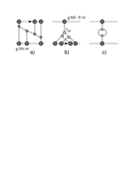
Figure 1: Examples of the Pomeron diagrams: ’net’ diagrams, which give the main contribution to nucleus-nucleus collisions (Fig. 1-a); the diagrams of the Balitsky-Kovchegov equation (Fig. 1-b); and the contribution to the Green function of the Pomeron(Fig. 1-c). The wavy lines describe the Pomeron Green function.

The natural generalization of Eq. (47) for diagram of Fig. 1-b is

$$N_{{Fig.~{}\ref{gen}}-b}\left(Y,b\right)\,\,=\,\,\frac{m^{2}}{4\pi}\int d^{2}b^{\prime}\bar{P}\left(y=Y,\boldsymbol{b}-\boldsymbol{b}^{\prime}\right)\Bigg{(}1-(1-P\left(Y,b^{\prime}\right))^{n}\Bigg{)}$$ (52)

which at $Y\to 0$ has the form

$$N_{{Fig.~{}\ref{gen}}-b}\left(Y=Y_{0},b\right)\,\,=\,\,\frac{m^{2}}{4\pi}\int d^{2}b^{\prime}\,\,p^{2}_{0}\,\,S\left(\boldsymbol{b}-\boldsymbol{b}^{\prime},m\right)\,S\left(\boldsymbol{b}^{\prime},m\right)\,\,=\,\,p^{2}_{0}\,\,n$$ (53)

where $n=\,\frac{m^{2}}{4\pi}\int d^{2}b\,S\left(\boldsymbol{b}-\boldsymbol{b}^{\prime},m\right)\,S\left(\boldsymbol{b}^{\prime},m\right)$ is the number of dipoles of size $1/m$ in the two interacting nucleons. It should be stressed that in Eq. (53) we assumed that the typical size of the dipole that is described by the new parton model is $2/m$. In principle, we can introduce this size as a new parameter whose value we will need to determine from comparison with the experimental data.

The expression for $z_{m}=e^{\Delta(1-p_{0})Y}$ sums diagrams of the type shown in Fig. 1-c . Since the triple Pomeron interaction does not induce any impact parameter dependence, we consider $p_{0}=\gamma={\rm Const}$ as a function of $b$.

Combining all the above, we obtain the following equation for the scattering amplitude:

$$A_{el}(Y,b)\,=\,1-\exp\Bigg{\{}\int\frac{m^{2}d^{2}b^{\prime}}{4\pi}\Bigg{[}\frac{1}{p_{0}}\Big{(}S(\alpha,\beta,z_{m})\,{\mathbf{+}}\,\alpha(p,\bar{p},z_{m})\Delta(1-p_{0})Y\Big{)}\,-\,\bar{P}\left(y=Y,\boldsymbol{b}-\boldsymbol{b}^{\prime}\right)\,P\left(Y,b^{\prime}\right)\Bigg{]}\Bigg{\}}$$ (54)

IV Comparison with experimental data

IV.1 Fitting $\sigma_{\rm tot},\sigma_{\rm el}$ and $B_{\rm el}$

As we have seen in the previous section, we introduce two dimensionless parameters: $\Delta$ - the intercept of the BFKL Pomeron, and $\gamma$ - the amplitude for dipole-dipole scattering at low energies. For $b$-dependence we suggested a specific form for $b$-dependence (see Eq. (50)) which is characterized by the dimensional factor $m$. All three parameters were determined by fitting to the experimental data. We choose to describe three observables: total and elastic cross section and the elastic slope. They have the following expressions through the partial amplitudes:

$$\sigma_{tot}\, = \,\,2\,\int d^{2}b\,\mbox{Im}A_{el}(Y,b);$$

$$\sigma_{el}\, = \,\,\,\int d^{2}b\,|A_{el}(Y,b)|^{2};$$

$$B_{el}\, = \,\frac{1}{2}\frac{\int b^{2}\,d^{2}b\,\mbox{Im}A_{el}(Y,b)}{\int d^{2}b\,\mbox{Im}A_{el}(Y,b)};$$ (55)

From Fig. 2 one can see that we can describe the data for $W\geq 1\,TeV$. The values of parameters are shown in Table 1. Comparing these parameters with the resulting curves in Fig. 2 we note that the shadowing corrections play an essential role. First, the corrections to the Green function of the Pomeron reduce the Pomeron intercept from $\Delta=0.644$ to $\Delta_{\rm dresssed}\,\,=\,\,0.35$. The other shadowing corrections lead to the effective intercept $\Delta_{\rm eff}\approx 0.07$.

$\Delta$	$p_{0}$	m (GeV)	$\chi^{2}$/d.o.f.
0.6488 $\pm$ 0.030	0.489 $\pm$ 0.030	0.867 $\pm$ 0.005	1.3

Table 1: Fitted parameters.

From Fig. 2 we see that we fail to describe the experimental data for $W<1\,TeV$. However, we would like to stress that we used a very naive model for the hadron structure. Our previous experienceGLMNI ; GLM2CH shows that we need to take into account the processes of diffraction production, which have been neglected in this model. Our main goal is to demonstrate that the suggested model is able to describe the experimental data at high energies.

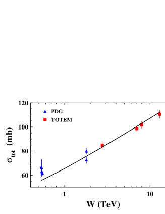
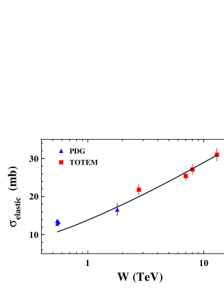
Fig. 2-a	Fig. 2-b	Fig. 2-c

Figure 2: The energy behaviour of $\sigma_{tot},\sigma_{el}$ and the slope $B_{el}$ for proton-proton scattering as predicted in our model. Data are taken from Refs.PDG ; TOTEMRHO . The data taken for the fit were for $W\,\geq\,$ 1 TeV.

IV.2 $A_{el}(Y,b)$

In Fig. 3 we plot the elastic scattering amplitude $A_{\rm el}\left(Y,b\right)$, as a function of the impact parameter. Note that this amplitude has reached the unitary limit 1 at $W=13\,TeV$ and shows the increasing with energy radius, of the interaction. For a comparison, we include in this picture the scattering amplitude, calculated in Balitsky-Kovchegov non-linear equation (see $A_{\rm el}(X)$). This amplitude is far from the unitarity limit and shows only a small increment with increasing energy.

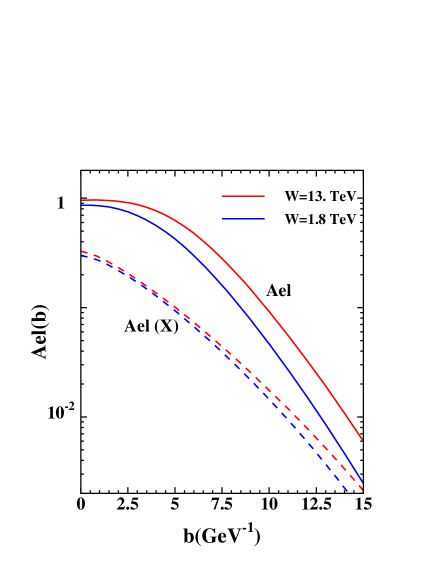
Figure 3: The elastic scattering amplitude versus $b$. $A_{\rm el}(X)$ is the amplitude from the Balitsky-Kovchegov equation( see Eq. (42)).

Such behaviour of the scattering amplitude $A_{\rm el}(X)$ reflects the fact that in our approach there is no fixed point (1,0) (or/ and (0,1)), as occurs in the Braun Hamiltonian, and the scattering of hadrons or nucleus cannot be reduced to BK evolution at high energies.

V Conclusions

In this paper we showed that the experimental data at high energies, can be described in the framework of the new parton model. The model is based on the Pomeron calculus in 1+1 space-time, suggested in Ref. AKLL , and on simple assumptions on the hadron structure, related to the impact parameter dependence of the scattering amplitude. This parton model stems from QCD, assuming that the unknown non-perturbative corrections lead to fixing the size of the interacting dipoles. The advantage of this approach is that it satisfies both the t-channel and s-channel unitarity, and can be used for summing all diagrams of the Pomeron interaction, including Pomeron loops. In other words, we can use this approach for all possible reactions: dilute-dilute (hadron-hadron), dilute-dense (hadron - nucleus) and dense-dense (nucleus-nucleus) parton systems scattering. Unfortunately, we are still far from tackling this problem in the framework of QCD effective theory at high energy (CGC /saturation approach).

We achieved quite good descriptions of the three experimental observables: $\sigma_{\rm tot}$,$\sigma_{\rm el}$ and $B_{\rm el}$, especially regarding the energy dependence of these observables. We consider this paper as the first attempt to show that the new parton model can be relevant to the discussion of the experimental data. In spite of the embryonic state of the theory of the quark-gluon confinement, we hope that our model can be viewed as the first step in the right direction regarding the theoretical description of the dilute-dilute parton system scattering at high energy at which, we believe, that such systems become dense.

We are aware that our model is very naive in the description of the hadron structure. We are planning to include diffraction production in our formalism, and to develop a theoretical approach in the framework of the new parton model, so as to be able to treat processes of multiparticle generation.

Acknowledgements.
We thank our colleagues at Tel Aviv University and UTFSM for encouraging discussions. This research was supported by the BSF grant 2012124, by Proyecto Basal FB 0821(Chile) , Fondecyt (Chile) grants 1140842 and 1180118 and by CONICYT grant PIA ACT1406.

References

- (1) E. Gotsman, E. Levin and I. Potashnikova, Phys. Lett. B 781 (2018) 155, [arXiv:1712.06992 [hep-ph]].
- (2) E. Gotsman, E. Levin and I. Potashnikova, Eur. Phys. J. C 77 (2017) no.9, 632, [arXiv:1706.07617 [hep-ph]].
- (3) E. Gotsman, E. Levin and U. Maor, Eur. Phys. J. C 75 (2015) 1, 18 [arXiv:1408.3811 [hep-ph]].
- (4) E. Gotsman, E. Levin and U. Maor, Eur. Phys. J. C 75 (2015) 5, 179 [arXiv:1502.05202 [hep-ph]].
- (5) E. Gotsman, E. Levin and U. Maor, Phys. Lett. B 746 (2015) 154 [arXiv:1503.04294 [hep-ph]].
- (6) E. Gotsman, E. Levin and U. Maor, Eur. Phys. J. C 75 (2015) 11, 518 [arXiv:1508.04236 [hep-ph]].
- (7) E. Gotsman, E. Levin and U. Maor, Eur. Phys. J. C 76 (2016) no.4, 177, [arXiv:1510.07249 [hep-ph]].
- (8) E. Gotsman, E. Levin, U. Maor and S. Tapia, Phys. Rev. D 93 (2016) no.7, 074029, [arXiv:1603.02143 [hep-ph]].
- (9) Y. V. Kovchegov and E. Levin Quantum chromodynamics at high energy Vol. 33 (Cambridge University Press, 2012).
- (10) T. Altinoluk, A. Kovner, E. Levin and M. Lublinsky, JHEP 1404 (2014) 075 [arXiv:1401.7431 [hep-ph]].
- (11) V. S. Fadin, E. A. Kuraev and L. N. Lipatov, Phys. Lett. B60, 50 (1975); E. A. Kuraev, L. N. Lipatov and V. S. Fadin, Sov. Phys. JETP 45, 199 (1977), [Zh. Eksp. Teor. Fiz.72,377(1977)]; I. I. Balitsky and L. N. Lipatov, Sov. J. Nucl. Phys. 28, 822 (1978), [Yad. Fiz.28,1597(1978)].
- (12) V. N. Gribov, Sov. Phys. JETP 26, 414 (1968) [Zh. Eksp. Teor. Fiz. 53, 654 (1967)].
- (13) V. A. Abramovsky, V. N. Gribov and O. V. Kancheli, Yad. Fiz. 18, 595 (1973) [Sov. J. Nucl. Phys. 18, 308 (1974)].
- (14) Y. V. Kovchegov and K. Tuchin, Phys. Rev. D 65, 074026 (2002) [arXiv:hep-ph/0111362].
- (15) J. Jalilian-Marian and Y. V. Kovchegov, Phys. Rev. D 70, 114017 (2004) [Erratum-ibid. D 71, 079901 (2005)] [arXiv:hep-ph/0405266].
- (16) A. H. Mueller and B. Patel, Nucl. Phys. B425 (1994) 471. A. H. Mueller and G. P. Salam, Nucl. Phys. B475, (1996) 293. [arXiv:hep-ph/9605302]. G. P. Salam, Nucl. Phys. B461 (1996) 512; E. Iancu and A. H. Mueller, Nucl. Phys. A730 (2004) 460 [arXiv:hep-ph/0308315]; 494 [arXiv:hep-ph/0309276].
- (17) M. A. Braun, Phys. Lett. B 483, 115 (2000); e-Print Archive:[hep-ph/0003004];Eur. Phys. J. C 33, 113 (2004) e-Print Archive: [hep-ph/0309293]; Phys. Lett. B 632, 297 (2006)
- (18) A. Kovner, E. Levin and M. Lublinsky, JHEP 1608 (2016) 031, [arXiv:1605.03251 [hep-ph]].
- (19) I. Balitsky, Nucl. Phys. B 463 (1996) 99, [hep-ph/9509348]. Phys. Rev. D60, 014020 (1999) [arXiv:hep-ph/9812311]; Y. V. Kovchegov, Phys. Rev. D60, 034008 (1999), [arXiv:hep-ph/9901281].
- (20) A. Kovner, M. Lublinsky and U. Wiedemann, JHEP 0706, 075 (2007), [arXiv: 0705.1713 [hep-ph]].
- (21) A. H. Mueller, Nucl. Phys. B 415 (1994) 373; ibid 437 (1995) 107.
- (22) E. Levin and M. Lublinsky, Nucl. Phys. A 730 (2004) 191, [hep-ph/0308279].
- (23) V. N. Gribov, Sov. J. Nucl. Phys. 9 (1969) 369 [Yad. Fiz. 9 (1969) 640].
- (24) R.P. Feynman, Phys. Rev. Lett. 23 (1969) 1415, Photon-Hadron Interactions - Reading 1972; V. N. Gribov, “Space-time description of hadron interactions at high-energies,” hep-ph/0006158.
- (25) R.J. Glauber, In: Lectures in Theor. Phys., v. 1, ed. W.E. Brittin and L.G. Duham. NY: Intersciences, 1959 .
- (26) A.H. Mueller, Nucl. Phys.B 335, ( 1990) 115.
-
(27)
L. McLerran and R. Venugopalan,
Phys. Rev. D49 (1994) 2233, 3352; D50 (1994) 2225;
D53 (1996) 458;
D59 (1999) 09400. - (28) I. Gradstein and I. Ryzhik, Table of Integrals, Series, and Products, Fifth Edition, Academic Press, London, 1994.
- (29) The Review of Particle Physics (2018), M. Tanabashi et al. (Particle Data Group), Phys. Rev. D 98, 030001 (2018).
- (30) G. Antchev et al. [TOTEM Collaboration], “First measurement of elastic, inelastic and total cross-section at TeV by TOTEM and overview of cross-section data at LHC energies,” CERN-EP-2017-321, CERN-EP-2017-321-V2 arXiv:1712.06153 [hep-ex]; “First determination of the parameter at probing the existence of a colourless three-gluon bound state,” CERN-EP-2017-335 , Submitted to: Phys.Rev.