Autoregressive Models for Matrix-Valued Time Series

Rong Chen, Han Xiao and Dan Yang

Rutgers University

Abstract

In finance, economics and many other fields, observations in a matrix form are often generated over time. For example, a set of key economic indicators are regularly reported in different countries every quarter. The observations at each quarter neatly form a matrix and are observed over consecutive quarters. Dynamic transport networks with observations generated on the edges can be formed as a matrix observed over time. Although it is natural to turn the matrix observations into long vectors, then use the standard vector time series models for analysis, it is often the case that the columns and rows of the matrix represent different types of structures that are closely interplayed. In this paper we follow the autoregression for modeling time series and propose a novel matrix autoregressive model in a bilinear form that maintains and utilizes the matrix structure to achieve a substantial dimensional reduction, as well as more interpretability. Probabilistic properties of the models are investigated. Estimation procedures with their theoretical properties are presented and demonstrated with simulated and real examples.

KEYWORDS: Autoregressive; Bilinear; Economic Indicators; Kronecker Product; Multivariate Time Series; Matrix-valued Time Series; Nearest Kronecker Product Projection; Prediction;

1 Introduction

Multivariate time series is a classical area in time series analysis, and has been extensively studied in the literature (see Hannan,, 1970; Lütkepohl,, 2005; Tsay,, 2014; Tiao and Box,, 1981, for an overview). Recently there has been an emerging interest in modeling high dimensional time series. Roughly speaking these works fall into two major categories: (i) vector autoregressive modeling with regularization (Davis et al.,, 2012; Basu and Michailidis,, 2015; Guo et al.,, 2015; Han et al.,, 2015, 2016; Nicholson et al.,, 2015; Song and Bickel,, 2011; Kock and Callot,, 2015; Negahban and Wainwright,, 2011; Nardi and Rinaldo,, 2011, among others), and (ii) statistical or dynamic factor models (Bai and Ng,, 2002; Forni et al.,, 2005; Lam et al.,, 2011; Lam and Yao,, 2012; Fan et al.,, 2013; Wang et al.,, 2019, among others). In most of these studies, the multiple observations at each time point are treated as a vector.

Although it has been conventional to treat multiple observations as a vector, often the inter-relationship among the time series exhibits some more structure. For example, Hallin and Liška, (2011) studied subpanel structures in multivariate time series, and Tsai and Tsay, (2010) considered group constraints among the time series. When the time series are collected under the intersections of two classifications, they naturally form matrices.

Figure 1: Time series of four economic indicators (first differenced 3 month interbank interest rate, GDP growth (log difference), Total Manufacture Production growth (log difference), and Total CPI growth from last period) from five countries.

In Figure 1, we plot four economic indicators from five countries, resulting in a $4\times 5$ matrix observed at each time point. In this example, the rows and columns correspond to different classifications (economic indicators and countries). Univariate time series analysis would deal with individual time series separately (e.g. US interest rate, or UK GDP). Panel time series analysis deals with one row at a time (e.g. interest rates of the five countries), or one column at a time (e.g. all economic indicators of US). Obviously every time series is related to all other time series in the matrix and we wish to model them jointly. It is reasonable to assume that the same economic indicator from different countries (the rows) form a strong relationship, and at the same time economic indicators from the same country (the columns) also naturally move together closely. Hence there is a strong structure in the relationship among the time series. If the matrices are concatenated into vectors, the underlying structure is lost with significant impacts on the model complexity and interpretations.

In this paper we propose to model the matrix-valued time series under the autoregressive framework with a bilinear form. Specifically, in this model, the conditional mean of the matrix observation at time $t$ is obtained by multiplying the previous observed matrix at time $t-1$ from both left and right by two autoregressive coefficient matrices. Let ${\boldsymbol{X}}_{t}$ be the $m\times n$ matrix observed at time $t$, our model takes the form

$$\boldsymbol{X}_{t}=\boldsymbol{A}\boldsymbol{X}_{t-1}\boldsymbol{B}^{\prime}+\boldsymbol{E}_{t},$$

It can be extended to involve the previous $p$ observed matrices to form an order $p$ autoregressive model. If it involves $p$ previously observed matrices, we call it the matrix autoregressive model of order $p$, with the acronym MAR($p$). Compared with the traditional vector autoregressive models, our approach has two advantages: (i) it keeps the original matrix structure, and its two coefficient matrices have corresponding interpretations; and (ii) it reduces the number of parameters in the model significantly.

Similar bilinear models have been used in regression settings. For instance, Wang et al., (2018) considered the regression with matrix-valued covariates for low-dimensional data. Zhao and Leng, (2014) studied the bilinear regression with sparse coefficient vectors under high-dimensional setting. Zhou et al., (2013) and Raskutti et al., (2015) mainly addressed the multi-linear regression with general tensor covariates.

A major objective of our model is to take full advantage of the original matrix structure, so that the model is naturally interpretable. A similar concern has emerged in the econometrics literature when studying a large panel of data consisting of blocks. Hierarchical or multi-level factor models have been introduced to capture both the within-block and between-block variations (Moench et al.,, 2013; Diebold et al.,, 2008; Giannone et al.,, 2008). Our model shares an interpretation as the hierarchical autoregression, which will be detailed in Section 2.1.

Our model leads to a substantial dimension reduction as compared with a direct vector autoregressive model ($m^{2}+n^{2}$ vs $m^{2}n^{2}$). However, when the matrix observations themselves have large dimensions, it would be desirable to impose further constraints so that a greater dimension reduction can be achieved. There are a number of possible approaches. First, we may require both ${\boldsymbol{A}}$ and ${\boldsymbol{B}}$ to be sparse, and carryout the estimation with a $\ell_{1}$ penalty. Second, we can consider the additional assumption that both ${\boldsymbol{A}}$ and ${\boldsymbol{B}}$ are of low ranks. If we fix one of ${\boldsymbol{A}}$ and ${\boldsymbol{B}}$ and consider the other as the parameter, the model can be viewed as a reduced rank regression (Anderson,, 1951; Izenman,, 1975). This second approach is also related to the recent work Wang et al., (2019), which studied the factor models for matrix-valued time series. These extensions are beyond the scope of this paper, and we would leave them for further research.

Since the error term in the matrix AR model is also a matrix, its (internal) covariances form a 4-dimensional tensor. Here we also consider to exploit the matrix structure to reduce the dimensionality of this covariance tensor, by separating the row-wise and column-wise dependencies of the error matrix.

In this paper we investigate some probabilistic properties of the proposed model. Several estimators for MAR(1) model are developed, with different computing algorithms, under different assumptions on the error covariance structure. Their asymptotic properties are investigated. We also compare the efficiencies of the estimators. In addition, the finite sample performances of the estimators are demonstrated through simulation studies. The matrix time series of four economic indicators from five countries, shown in Figure 1, is analyzed in detail.

The rest of the paper is organized as follows. We introduce the autoregressive model for matrix-valued time series in Section 2, along with some of its probabilistic properties. The estimation procedures are presented in Section 3. Statistical inferences and the asymptotic properties of the estimators will be considered in Section 4. Numerical studies are carried out in Section 5. Section 6 contains a short summary. All the proofs are collected in Appendix.

2 Autoregressive Model for Matrix-Valued Time Series

Consider a time series of length $T$, in which at each time $t$, a $m\times n$ matrix $\boldsymbol{X}_{t}$ is observed. Here we use $\boldsymbol{X}$ in boldface to emphasize the fact that it is a matrix. Let $\mathrm{vec}(\cdot)$ be the vectorization of a matrix by stacking its columns. The traditional vector autoregressive model (VAR) of order 1 is directly applicable for $\mathrm{vec}({\boldsymbol{X}}_{t})$. That is,

$$\mathrm{vec}(\boldsymbol{X}_{t})=\Phi\mathrm{vec}({\boldsymbol{X}}_{t-1})+\mathrm{vec}({\boldsymbol{E}}_{t}).$$ (1)

It is immediately seen that the roles of rows and columns are mixed in the VAR model in (1). Using the example shown in Figure 1, the VAR model in (1) fails to recognize the strong connections within the columns (same country) and within the rows (same indicator). The (large) $mn\times mn$ coefficient matrix $\Phi$ does not have any assumed structure; and the model does not fully utilize the matrix structure, or any prior knowledge of the potential relationship among the time series. The coefficient matrix $\Phi$ is also very difficult to interpret.

To overcome the drawback of the direct VAR modeling that requires vectorization, and to take advantage of the original matrix structure, we propose the matrix autoregressive model (of order 1), denoted by MAR(1), in the form

$$\boldsymbol{X}_{t}=\boldsymbol{A}\boldsymbol{X}_{t-1}\boldsymbol{B}^{\prime}+\boldsymbol{E}_{t},$$ (2)

where $\boldsymbol{A}=(a_{ij})$ and $\boldsymbol{B}=(b_{ij})$ are $m\times m$ and $n\times n$ autoregressive coefficient matrices, and $\boldsymbol{E}_{t}=(e_{t,ij})$ is a $m\times n$ matrix white noise. Clearly the model can be extended to an order $p$ model in the form

$$\boldsymbol{X}_{t}=\boldsymbol{A}_{1}\boldsymbol{X}_{t-1}\boldsymbol{B}_{1}^{\prime}+\cdots+\boldsymbol{A}_{p}\boldsymbol{X}_{t-p}\boldsymbol{B}_{p}^{\prime}+\boldsymbol{E}_{t}.$$

We will defer the interpretations of ${\boldsymbol{A}}$ and ${\boldsymbol{B}}$ in (2) to Section 2.1.

The MAR(1) model in (2) can be represented in the form of a vector autoregressive model

$$\mathrm{vec}(\boldsymbol{X}_{t})=({\boldsymbol{B}}\otimes{\boldsymbol{A}})\mathrm{vec}({\boldsymbol{X}}_{t-1})+\mathrm{vec}({\boldsymbol{E}}_{t}),$$ (3)

where $\otimes$ denotes the matrix Kronecker product. A thorough discussion of the Kronecker product and its relationship with linear matrix equations can be found in Chapter 4 of Horn and Johnson, (1994). In the Appendix, we collect some basic properties of the Kronecker product in Proposition 7. The representation (3) means that the MAR(1) model can be viewed as a special case of the classical VAR(1) model in (1), with its autoregressive coefficient matrix given by a Kronecker product. On the other hand, comparing (1) and (3), we see that the MAR(1) requires $m^{2}+n^{2}$ coefficients as the entries of ${\boldsymbol{A}}$ and ${\boldsymbol{B}}$, while an unrestricted VAR(1) needs $m^{2}n^{2}$ coefficients for $\Phi$. Apparently the latter can be much larger when both $m$ and $n$ are large.

There is an obvious identifiability issue with the MAR(1) model in (2), regarding the two coefficient matrices ${\boldsymbol{A}}$ and ${\boldsymbol{B}}$. The model remains unchanged if the two matrices ${\boldsymbol{A}}$ and ${\boldsymbol{B}}$ are divided and multiplied by the same nonzero constant respectively. To avoid ambiguity, we use the convention that ${\boldsymbol{A}}$ is normalized so that its Frobenius norm is one. On the other hand, the uniqueness always holds for the Kronecker product ${\boldsymbol{B}}\otimes{\boldsymbol{A}}$.

The error matrix sequence $\{{\boldsymbol{E}}_{t}\}$ is assumed to be a matrix white noise, i.e. there is no correlation between ${\boldsymbol{E}}_{t}$ and ${\boldsymbol{E}}_{s}$ as long as $t\neq s$. But ${\boldsymbol{E}}_{t}$ is still allowed to have concurrent correlations among its own entries. As a matrix, its covariances form a 4-dimensional tensor, which is difficult to express. In the following we will discuss it in the form of $\Sigma=\operatorname{Cov}(\mathrm{vec}({\boldsymbol{E}}_{t}))$, a $(mn)\times(mn)$ matrix. As the simplest case, we may assume the entries of ${\boldsymbol{E}}_{t}$ are independent so that $\operatorname{Cov}(\mathrm{vec}({\boldsymbol{E}}_{t}))$ is a diagonal matrix; and in general, we allow them to have arbitrary correlations. We also consider a structured covariance matrix

$$\operatorname{Cov}(\mathrm{vec}({\boldsymbol{E}}_{t}))=\Sigma_{c}\otimes\Sigma_{r},$$ (4)

where $\Sigma_{r}$ and $\Sigma_{c}$ are $m\times m$ and $n\times n$ symmetric positive definite matrices. Under normality, this is equivalent to assuming ${\boldsymbol{E}}_{t}=\Sigma_{r}^{1/2}\boldsymbol{Z}_{t}\Sigma_{c}^{1/2}$, where all the entries of $\boldsymbol{Z}_{t}$ are independent, and following the standard Normal distribution. Therefore, $\Sigma_{r}$ corresponds to row-wise covariances and $\Sigma_{c}$ introduces column-wise covariances.

Remarks:   There are many possible extensions of the model. For example, the model can be extended to have multiple lag-one autoregressive terms. That is

$$\boldsymbol{X}_{t}=\boldsymbol{A}_{1}\boldsymbol{X}_{t-1}\boldsymbol{B}_{1}^{\prime}+\cdots+\boldsymbol{A}_{d}\boldsymbol{X}_{t-1}\boldsymbol{B}_{d}^{\prime}+\boldsymbol{E}_{t}.$$ (5)

This is still an order-1 autoregressive model, but with more parallel terms. In the stacked vector form, it corresponds to

$$\mathrm{vec}(\boldsymbol{X}_{t})=\left(\sum_{i=1}^{d}{\boldsymbol{B}}_{i}\otimes{\boldsymbol{A}}_{i}\right)\mathrm{vec}({\boldsymbol{X}}_{t-1})+\mathrm{vec}({\boldsymbol{E}}_{t}).$$

Such a structure provides more flexibility to capture the different interactions among rows and columns of the matrix time series, though it becomes more challenging, since there is obviously a more severe identifiability issue.

In this paper we focus on MAR(1) model (2) in all our discussions. Extensions will be investigated elsewhere.

2.1 Model interpretations

The MAR(1) model is not a straightforward model. A thorough discussion of the interpretations of its coefficient matrices is needed. Here we offer interpretations from three different angles.

First, in model (2), the left matrix $\boldsymbol{A}$ reflects row-wise interactions, and the right matrix $\boldsymbol{B}^{\prime}$ introduces column-wise dependence, and therefore the conditional mean in (2) combines the row-wise and column-wise interactions. It is easier to see how the coefficient matrices ${\boldsymbol{A}}$ and ${\boldsymbol{B}}$ reflects the row and column structures by looking at a few special cases.

To isolate the effect from the bilinear form in (2), let us assume ${\boldsymbol{A}}={\boldsymbol{I}}$. Then the model reduces to

$${\boldsymbol{X}}_{t}={\boldsymbol{X}}_{t-1}{\boldsymbol{B}}^{\prime}+{\boldsymbol{E}}_{t}.$$

Consider the example shown in Figure 1, using columns for countries and rows for economic indicators. The conditional expectation of the first column of ${\boldsymbol{X}}_{t}$ is given by

USAUSADEUCAN

$$\begin{pmatrix}\hbox{Int}\\ \hbox{GDP}\\ \hbox{Prod}\\ \hbox{CPI}\end{pmatrix}_{t}=b_{11}\begin{pmatrix}\hbox{Int}\\ \hbox{GDP}\\ \hbox{Prod}\\ \hbox{CPI}\end{pmatrix}_{t-1}+b_{12}\begin{pmatrix}\hbox{Int}\\ \hbox{GDP}\\ \hbox{Prod}\\ \hbox{CPI}\end{pmatrix}_{t-1}+\cdots+b_{1n}\begin{pmatrix}\hbox{Int}\\ \hbox{GDP}\\ \hbox{Prod}\\ \hbox{CPI}\end{pmatrix}_{t-1},$$

which means that at time $t$, the conditional expectation of an economic indicator of one country is a linear combinations of the same indicator from all countries at $t-1$, and this linear combination is the same for different indicators. Therefore, this model (and ${\boldsymbol{B}}$) captures the column-wise interactions, i.e. interactions among the countries. However, the interactions are refrained within each indicator. There are no interactions among the indicators.

On the other hand, if we let ${\boldsymbol{B}}={\boldsymbol{I}}$ in model (2), then a similar interpretation can be obtained, where the matrix ${\boldsymbol{A}}$ reflects the row-wise interactions, i.e. interactions among the economic indicators within each country. There are no interactions among the countries.

Second, we can interpret the model from a row-wise and column-wise VAR model point of view. For example, if ${\boldsymbol{B}}={\boldsymbol{I}}$, then the model becomes

$${\boldsymbol{X}}_{t}={\boldsymbol{A}}{\boldsymbol{X}}_{t-1}+{\boldsymbol{E}}_{t}.$$

In this case, each column of ${\boldsymbol{X}}_{t}$ follows

$${\boldsymbol{X}}_{t,\cdot j}={\boldsymbol{A}}{\boldsymbol{X}}_{t-1,\cdot j}+{\boldsymbol{E}}_{t,{\cdot j}},\mbox{ \ \ }j=1,\ldots n.$$

That is, each column of ${\boldsymbol{X}}_{t}$ follows the same VAR(1) model of dimension $m$. Specifically, for the first two columns in the example of Figure 1, the models are

    USAUSAUSA     DEUDEUDEU

$$\begin{pmatrix}\hbox{Int}\\ \hbox{GDP}\\ \hbox{Prod}\\ \hbox{CPI}\end{pmatrix}_{t}={\boldsymbol{A}}\begin{pmatrix}\hbox{Int}\\ \hbox{GDP}\\ \hbox{Prod}\\ \hbox{CPI}\end{pmatrix}_{t-1}+\begin{pmatrix}\hbox{e\_Int}\\ \hbox{e\_GDP}\\ \hbox{e\_Prod}\\ \hbox{e\_CPI}\end{pmatrix}_{t} \begin{pmatrix}\hbox{Int}\\ \hbox{GDP}\\ \hbox{Prod}\\ \hbox{CPI}\end{pmatrix}_{t}={\boldsymbol{A}}\begin{pmatrix}\hbox{Int}\\ \hbox{GDP}\\ \hbox{Prod}\\ \hbox{CPI}\end{pmatrix}_{t-1}+\begin{pmatrix}\hbox{e\_Int}\\ \hbox{e\_GDP}\\ \hbox{e\_Prod}\\ \hbox{e\_CPI}\end{pmatrix}_{t}$$ and

In other words, for each country, its economic indicators follow a VAR(1) model (of its own past) of dimension $m$; and different countries would follow the same VAR(1) model.

If ${\boldsymbol{A}}={\boldsymbol{I}}$, then

$${\boldsymbol{X}}_{t}={\boldsymbol{X}}_{t-1}{\boldsymbol{B}}^{\prime}+{\boldsymbol{E}}_{t}.$$

In this case, each row of ${\boldsymbol{X}}_{t}$ (same indicator from different countries) would follow a VAR(1) model. And the coefficient matrices corresponding to different rows would be the same.

Obviously both models ${\boldsymbol{X}}_{t}={\boldsymbol{A}}{\boldsymbol{X}}_{t-1}+{\boldsymbol{E}}_{t}$ and ${\boldsymbol{X}}_{t}={\boldsymbol{X}}_{t-1}{\boldsymbol{B}}^{\prime}+{\boldsymbol{E}}_{t}$ are too restrictive. It is difficult to reason that Germany’s economic indicators follow the same model as the US’s, and there is no interaction between Germany and US. There are two possible ways to add flexibility. One can assume an additive interaction structure to make the model as

$${\boldsymbol{X}}_{t}={\boldsymbol{A}}{\boldsymbol{X}}_{t-1}+{\boldsymbol{X}}_{t-1}{\boldsymbol{B}}^{\prime}+{\boldsymbol{E}}_{t},$$

which is essentially a special case of the multi-term model in (5) with $d=2$ and ${\boldsymbol{B}}_{1}={\boldsymbol{I}}$ and ${\boldsymbol{A}}_{2}={\boldsymbol{I}}$. Or we can assume a one-term multiplicative interaction structure, which leads to MAR(1). Of course, one can also use

$${\boldsymbol{X}}_{t}={\boldsymbol{A}}_{1}{\boldsymbol{X}}_{t-1}+{\boldsymbol{X}}_{t-1}{\boldsymbol{B}}_{1}^{\prime}+{\boldsymbol{A}}_{2}{\boldsymbol{X}}_{t-1}{\boldsymbol{B}}_{2}^{\prime}+{\boldsymbol{E}}_{t},$$

similar to the model with main effects plus two-way interactions. In this paper we choose to work on MAR(1) in (2).

The third way to interpret MAR(1) is through a defined hierarchical structure. Multi-level or hierarchical factor models have been introduced in the econometric literature to study a large panel of data consisting of blocks or even sub-blocks (Moench et al.,, 2013; Diebold et al.,, 2008; Giannone et al.,, 2008). Here we illustrate that our model shares a similar interpretation as hierarchical autoregression. Let ${\boldsymbol{Y}}_{t-1}={\boldsymbol{X}}_{t-1}{\boldsymbol{B}}^{\prime}$. It would be the prediction of ${\boldsymbol{X}}_{t}$ (or the conditional mean) if ${\boldsymbol{A}}={\boldsymbol{I}}$. Since each column of ${\boldsymbol{Y}}_{t-1}$ is based on the linear combination of all columns of ${\boldsymbol{X}}_{t-1}$ with no row (indicator) interaction, we can view each entry in ${\boldsymbol{Y}}_{t-1}$ as the globally adjusted indicator. For example, ${\boldsymbol{Y}}_{t-1,GDP,US}$ is a linear combination of the GDPs of all countries at time $t-1$. Next, we consider ${\boldsymbol{Z}}_{t-1}={\boldsymbol{A}}{\boldsymbol{Y}}_{t-1}$. This would be the prediction of ${\boldsymbol{X}}_{t}$ if the model is ${\boldsymbol{X}}_{t}={\boldsymbol{A}}{\boldsymbol{Y}}_{t-1}+{\boldsymbol{E}}_{t}$. It replaces each entry (indicator) in ${\boldsymbol{X}}_{t-1}$ by its corresponding globally adjusted indicator in ${\boldsymbol{Y}}_{t-1}$. Each entry in ${\boldsymbol{Z}}_{t-1}$ is a linear combination of the adjusted indicators from the same country. For example, ${\boldsymbol{Z}}_{t-1,GDP,US}$ is a linear combination of ${\boldsymbol{Y}}_{t-1,GDP,US}$, ${\boldsymbol{Y}}_{t-1,INT,US}$ etc. It can be viewed as a second adjustment by other indicators (within the same country). Putting everything together, we have

$${\boldsymbol{X}}_{t}={\boldsymbol{Z}}_{t-1}+{\boldsymbol{E}}_{t}={{\boldsymbol{A}}{\boldsymbol{Y}}_{t-1}}+{\boldsymbol{E}}_{t}={\boldsymbol{A}}{\boldsymbol{X}}_{t-1}{\boldsymbol{B}}^{\prime}+{\boldsymbol{E}}_{t}.$$

Note that, if ${\boldsymbol{X}}_{t}$ follows the MAR(1) in (2), each entry $x_{t,ij}$ in ${\boldsymbol{X}}_{t}$ follows

$${x_{t,ij}=\sum_{k_{1}=1}^{m}\sum_{k_{2}=1}^{n}a_{ik_{1}}x_{t-1,k_{1}k_{2}}b_{jk_{2}}+e_{t,ij}}.$$

Hence $x_{t,ij}$ is controlled only by $i$-th row of ${\boldsymbol{A}}$ and $j$-th column of ${\boldsymbol{B}}^{\prime}$. In the example of Figure 1, the $i$-th row of ${\boldsymbol{A}}$ can be viewed as the coefficient corresponding to $i$-th indicator and the $j$-th column of ${\boldsymbol{B}}^{\prime}$ as the coefficient corresponding to the $j$-th country. Their values can be interpreted, as we will demonstrate in the real example in Section 4.

The error covariance matrix $\operatorname{Cov}(\mathrm{vec}({\boldsymbol{E}}_{t}))=\Sigma_{c}\otimes\Sigma_{r}$ in (4), which consists of all pairwise covariances $\operatorname{Cov}(e_{t,ij},e_{t,kl})=\sigma_{c,jl}\sigma_{r,ik}$, has a similar interpretation. For example, if $\Sigma_{r}={\boldsymbol{I}}$, then ${\boldsymbol{E}}_{t}={\boldsymbol{Z}}\Sigma_{c}^{1/2}$, which implies that the $\Sigma_{c}$ matrix captures the concurrent dependence of the columns of shocks in ${\boldsymbol{E}}_{t}$. Note that each row of ${\boldsymbol{E}}_{t}$ in this case is ${\boldsymbol{E}}_{t,i\cdot}={\boldsymbol{Z}}_{t,i\cdot}\Sigma_{c}^{1/2}$. Hence $\operatorname{Cov}({\boldsymbol{E}}_{t,i\cdot})=\Sigma_{c}$ for all rows $i=1,\dots,m$, and therefore $\Sigma_{c}$ captures the covariance among the (column) elements in each row. In parallel, $\Sigma_{r}$ captures the concurrent dependence among the rows of shocks in ${\boldsymbol{E}}_{t}$.

2.2 Probabilistic properties of MAR(1)

For any square matrix $\boldsymbol{C}$, we use $\rho(\boldsymbol{C})$ to denote its spectral radius, which is defined as the maximum modulus of the (complex) eigenvalues of $\boldsymbol{C}$. Since the MAR(1) model can be represented in the form (3), we see that (2) admits a causal and stationary solution if the spectral radius of ${\boldsymbol{B}}\otimes{\boldsymbol{A}}$, which is the product of the spectral radii of ${\boldsymbol{A}}$ and ${\boldsymbol{B}}$, is strictly less than 1. Hence we have

Proposition 1.

If $\rho({\boldsymbol{A}})\cdot\rho({\boldsymbol{B}})<1$, then the MAR(1) model (2) is stationary and causal.

The detailed proof of the proposition is given in the Appendix.

We remark that the property of being “stationary and causal” is referred to as being “stable” in Lütkepohl, (2005). Here we follow the terminology and definitions used in Brockwell and Davis, (1991). The condition $\rho({\boldsymbol{A}})\cdot\rho({\boldsymbol{B}})<1$ will be referred to as the causality condition in the sequel.

When the condition of Proposition 1 is fulfilled, the MAR(1) model in (2) has the following causal representation after vectorization:

$$\mathrm{vec}({\boldsymbol{X}}_{t})=\sum_{k=0}^{\infty}{\left({\boldsymbol{B}}^{k}\otimes{\boldsymbol{A}}^{k}\right)}\mathrm{vec}({\boldsymbol{E}}_{t-k}).$$ (6)

It follows that the autocovariance matrices of (2) is given by

$$\Gamma_{k}:=\operatorname{Cov}(\mathrm{vec}({\boldsymbol{X}}_{t}),\mathrm{vec}({\boldsymbol{X}}_{t-k}))=\sum_{l=0}^{\infty}{\left({\boldsymbol{B}}^{k+l}\otimes{\boldsymbol{A}}^{k+l}\right)\Sigma\left({\boldsymbol{B}}^{l}\otimes{\boldsymbol{A}}^{l}\right)^{\prime}},\quad k\geq 0,$$ (7)

where $\Sigma$ is the covariance matrix of $\mathrm{vec}({\boldsymbol{E}}_{t})$. The condition $\rho({\boldsymbol{A}})\cdot\rho({\boldsymbol{B}})<1$ guarantees that the infinite matrix series is absolutely summable.

It is known that a causal and a non-causal VAR(1) can lead to equivalent models under Gaussianity (Hannan,, 1970). However, if the parameter space of (1) is restricted to $\Theta:=\{(\Phi,\Sigma):\;\rho(\Phi)<1,\hbox{ and }\Sigma\hbox{ is nonsingular}\}$, then the VAR(1) model (1) is identifiable in the sense that if two sets of parameters $(\Phi_{1},\Sigma_{1})\in\Theta$ and $(\Phi_{2},\Sigma_{2})\in\Theta$ generate the same autocovariance functions (7), then they must be identical. To see this, first note that under causality, the best linear prediction of $\mathrm{vec}({\boldsymbol{X}}_{t})$ by $\mathrm{vec}({\boldsymbol{X}}_{t-1})$ is $\Phi_{i}\mathrm{vec}({\boldsymbol{X}}_{t-1})$, so the prediction error covariance matrices $\Sigma_{1}$ and $\Sigma_{2}$ must be the same. Second, under causality, $\Gamma_{1}=\Phi_{i}\Gamma_{0}$. Since $\Sigma_{1}=\Sigma_{2}$ are nonsingular, so is $\Gamma_{0}$. Therefore, both $\Phi_{1}$ and $\Phi_{2}$ would equal to $\Gamma_{1}\Gamma_{0}^{-1}$. Now we consider the identifiability regarding ${\boldsymbol{A}}$ and ${\boldsymbol{B}}$ over the parameter space $\{({\boldsymbol{A}},{\boldsymbol{B}}):\;\|{\boldsymbol{A}}\|_{F}=1,\;\|{\boldsymbol{B}}\|_{F}>0\}$. If ${\boldsymbol{B}}_{1}\otimes{\boldsymbol{A}}_{1}={\boldsymbol{B}}_{2}\otimes{\boldsymbol{A}}_{2}$, then $\boldsymbol{M}:=\mathrm{vec}({\boldsymbol{A}}_{1})\mathrm{vec}({\boldsymbol{B}}_{1})^{\prime}=\mathrm{vec}({\boldsymbol{A}}_{2})\mathrm{vec}({\boldsymbol{B}}_{2})^{\prime}$. Since $\boldsymbol{M}$ is a nonzero matrix, and $\|{\boldsymbol{A}}_{1}\|_{F}=\|{\boldsymbol{A}}_{2}\|_{F}=1$, the uniqueness of the singular value decomposition of $\boldsymbol{M}$ guarantees that $({\boldsymbol{A}}_{1},{\boldsymbol{B}}_{1})=\pm({\boldsymbol{A}}_{2},{\boldsymbol{B}}_{2})$, giving the desired identifiability up to a sign change. When $\Sigma$ is defined with the Kronecker product form (4), the identifiability regarding parameters $\Sigma_{r}$ and $\Sigma_{c}$ can be similarly showed if we require both of them to be nonsingular, and $\|\Sigma_{r}\|_{F}=1$.

We discuss the impulse response function with orthogonal innovations (oIRF) of the MAR(1) model. Since MAR(1) is a special case of VAR(1), we follow the definition given in Section 2.10 of Tsay, (2014). However, the standard approach requires fixing the order under which the innovations are orthogonalized, which is specially difficult to determine for matrix innovations. In this paper we adopt a simpler strategy. To obtain the oIRF with a shock at $(i,j)$-th series, we will put that series as the first series in the vectorized VAR model, and all other innovations will be orthogonalized with the $(i,j)$-th innovation fixed. The oIRF obtained this way actually does not depend on the order of the rest variables and its formulation is simple without the need to perform Cholesky decomposition. We will call the oIRF obtained this way the shock-first impulse response function with orthogonal innovations (s1-oIRF). Specifically, let $\Sigma[\,,i]$ be the $i$-th column of $\Sigma$, and $\sigma_{ij}$ be the $(i,j)$-th entry of $\Sigma$. Then the s1-oIRF of a unit standard deviation change in $e_{t,ij}$ (which is $\sigma^{1/2}_{m(j-1)+i,m(j-1)+i}$) is given by, in the vectorized form of the original matrix,

$${\boldsymbol{F}}_{i,j}(k)=\left({\boldsymbol{B}}^{k}\otimes{\boldsymbol{A}}^{k}\right)\Sigma[\,,m(j-1)+i].$$ (8)

Note that the s1-oIRF in (8) depends on the series to which the shock occurs, just as the standard oIRF depends on the order of variables. The accumulated s1-oIRF is in the form

$$\tilde{{\boldsymbol{F}}}_{i,j}(K)=\left(\sum_{k=0}^{K}{\boldsymbol{B}}^{k}\otimes{\boldsymbol{A}}^{k}\right)\Sigma[\,,m(j-1)+i].$$

This type of impulse response function exhibits a special structure if $\Sigma$ has the Kronecker product form (4). Let $\Sigma_{r,\cdot i}$ and $\Sigma_{c,\cdot i}$ be the $i$-th columns of $\Sigma_{r}$ and $\Sigma_{c}$, respectively. Then the effect of a unit standard deviation change in $e_{t,ij}$ on the future $\mathrm{vec}({\boldsymbol{X}}_{t+k})$ is given by $({\boldsymbol{B}}^{k}\Sigma_{c,\cdot j})\otimes({\boldsymbol{A}}^{k}\Sigma_{r,\cdot i})$.

To see the impact of this formulation, consider the case that a one-standard deviation shock occurs at $(1,1)$ series. Let $f^{c}_{i}(k)=({\boldsymbol{B}}^{k}\Sigma_{c,\cdot 1})[i]$, the $i$-th element of ${\boldsymbol{B}}^{k}\Sigma_{c,\cdot 1}$ and $f^{r}_{j}(k)=({\boldsymbol{A}}^{k}\Sigma_{r,\cdot 1})[j]$, the $j$-th element of ${\boldsymbol{A}}^{k}\Sigma_{r,\cdot 1}$. Then the impulse response function of $(i,j)$-th series at lag $k$ is

$$f_{i,j}(k)=f^{r}_{i}(k)f^{c}_{j}(k)=({\boldsymbol{A}}^{k}\Sigma_{r,\cdot 1})[i]\cdot({\boldsymbol{B}}^{k}\Sigma_{c,\cdot 1})[j].$$

We further let ${\boldsymbol{f}}^{r}(k)=[f^{r}_{1}(k),\ldots,f^{r}_{m}(k)]^{\prime}$, and ${\boldsymbol{f}}^{c}(k)=[f^{c}_{1}(k),\ldots,f^{c}_{n}(k)]^{\prime}$. (We use the boldfaced ${\boldsymbol{f}}(\cdot)$ here to emphesize it is a vector of functions.) We can view ${\boldsymbol{f}}^{r}(k)$ as the column response function and ${\boldsymbol{f}}^{c}(k)$ as the row response function. Using the example shown in Figure 1, if there is a unit standard deviation shock in the interest rate of US (location $(1,1)$ in the matrix), then its lag $k$ effect on the four economic indicators for $j$-th country is

$$[f_{1,j}(k),f_{2,j}(k),f_{3,j}(k),f_{4,j}(k)]^{\prime}=[f^{r}_{1}(k),f^{r}_{2}(k),f^{r}_{3}(k),f^{r}_{4}(k)]^{\prime}f^{c}_{j}(k)=f^{c}_{j}(k)\cdot{\boldsymbol{f}}^{r}(k),$$

which has the following interpretations. The effect of the shock on four economic indicators in the same $j$-th country, a 4-dimensional vector $[f_{1,j}(k),f_{2,j}(k),f_{3,j}(k),f_{4,j}(k)]^{\prime}$, is proportional to the vector ${\boldsymbol{f}}^{r}(k)$, for all countries $1\leq j\leq 5$. Hence the five (4-dimensional economic indicator) vectors corresponding to the five countries are parellel to each other and only differ by the multiplier $f^{c}_{j}(k)$. This form of impulse response function implies that the economies of different countries have a co-movement as responses to a shock, but the impacts on different countries are of different scales. Similarly, we have

$$[f_{i,1}(k),\ldots,f_{i,5}(k)]=f^{r}_{i}(k)\cdot[f^{c}_{1}(k),\ldots,f^{c}_{5}(k)]=f^{r}_{i}(k)\cdot[{\boldsymbol{f}}^{c}(k)]^{\prime},\quad 1\leq i\leq 4.$$

That is, the effect on five countries regarding each economic indicator, which is a 5-dimensional row vector, is proportional to ${\boldsymbol{f}}^{c}(k)$, and the four vectors corresponding to four indicators only differ by lengths $f^{r}_{i}(k)$.

In general, for a shock that occurs at location $(i,j)$, the lag-$k$ row and column response functions are ${\boldsymbol{f}}^{c,j}(k)={\boldsymbol{B}}^{k}\Sigma_{c,\cdot j}$ and ${\boldsymbol{f}}^{r,i}(k)={\boldsymbol{A}}^{k}\Sigma_{r,\cdot i}$, respectively. In fact, the response function in matrix form in this case is given by the rank-one matrix:

$$\hbox{\bf F}_{i,j}(k)={\boldsymbol{f}}^{r,i}(k)[{\boldsymbol{f}}^{c,j}(k)]^{\prime}.$$

3 Estimation

3.1 Projection method

To estimate the coefficient matrices ${\boldsymbol{A}}$ and ${\boldsymbol{B}}$, our first approach is to view the MAR(1) model in (2) as the structured VAR(1) model in (3). We first obtain the maximum likelihood estimate or the least square estimate $\hat{\Phi}$ of $\Phi$ in (1) without the structure constraint, then we find the estimators by projecting $\hat{\Phi}$ onto the space of Kronecker products under the Frobenius norm:

$$(\hat{\boldsymbol{A}}_{1},\hat{\boldsymbol{B}}_{1})=\arg\min_{{\boldsymbol{A}},{\boldsymbol{B}}}\|\hat{\Phi}-{\boldsymbol{B}}\otimes{\boldsymbol{A}}\|_{F}^{2}.$$ (9)

This minimization problem is called the nearest Kronecker product (NKP) problem in matrix computation (Van Loan and Pitsianis,, 1993; Van Loan,, 2000). It turns out that an explicit solution exists, which can be obtained through a singular value decomposition (SVD) of a rearranged version of $\hat{\Phi}$.

Note that the set of all entries in ${\boldsymbol{B}}\otimes{\boldsymbol{A}}$ is exactly the same as the set of all entries in $\mathrm{vec}({\boldsymbol{A}})\mathrm{vec}({\boldsymbol{B}})^{\prime}$. The two matrices have the same set of elements, and only differ by the placement of the elements in the matrices. Define a re-arrangement operator $\mathcal{G}:\mathbb{R}^{mn}\times\mathbb{R}^{{mn}}\rightarrow\mathbb{R}^{{m^{2}}}\times\mathbb{R}^{{n^{2}}}$ such that

$${\cal G}({\boldsymbol{B}}\otimes{\boldsymbol{A}})=\mathrm{vec}({\boldsymbol{A}})\mathrm{vec}({\boldsymbol{B}})^{\prime}.$$

It is easy to see that the operator is a linear operator such that ${\cal G}({\boldsymbol{C}}_{1}+{\boldsymbol{C}}_{2})={\cal G}({\boldsymbol{C}}_{1})+{\cal G}({\boldsymbol{C}}_{2})$. We also note that the Frobenius norm of a matrix only depends on the elements in the matrix, but not the arrangement, hence $||{\cal G}({\boldsymbol{C}})||_{F}=||{\boldsymbol{C}}||_{F}$. Then we have

$$\min_{{\boldsymbol{A}},{\boldsymbol{B}}}\|\hat{\Phi}-{\boldsymbol{B}}\otimes{\boldsymbol{A}}\|_{F}^{2} = \min_{{\boldsymbol{A}},{\boldsymbol{B}}}\|{\cal G}(\hat{\Phi})-{\cal G}({\boldsymbol{B}}\otimes{\boldsymbol{A}})\|_{F}^{2}$$

$$= \min_{{\boldsymbol{A}},{\boldsymbol{B}}}\|{\cal G}(\hat{\Phi})-\mathrm{vec}({\boldsymbol{A}})\mathrm{vec}({\boldsymbol{B}})^{\prime}\|_{F}^{2}$$

$$= \min_{{\boldsymbol{A}},{\boldsymbol{B}}}\|{\tilde{\Phi}}-\mathrm{vec}({\boldsymbol{A}})\mathrm{vec}({\boldsymbol{B}})^{\prime}\|_{F}^{2},$$

where ${\tilde{\Phi}}={\cal G}(\hat{\Phi})$ is the re-arranged $\hat{\Phi}$. It follows that the solution of (9) can be obtained through

$$\mathrm{vec}(\hat{\boldsymbol{A}})\mathrm{vec}(\hat{\boldsymbol{B}})^{\prime}=d_{1}\boldsymbol{u}_{1}\boldsymbol{v}_{1}^{\prime},$$

where $d_{1}$ is the largest singular value of $\tilde{\Phi}$, and $\boldsymbol{u}_{1}$ and $\boldsymbol{v}_{1}$ are the corresponding first left and right singular vectors, respectively. By converting the vectors into matrices, we obtain corresponding estimators of ${\boldsymbol{A}}$ and ${\boldsymbol{B}}$, denoted by $\hat{\boldsymbol{A}}_{1}$ and $\hat{\boldsymbol{B}}_{1}$, with the normalization that $||\hat{{\boldsymbol{A}}}_{1}||_{F}=1$. We call them projection estimators, and will use the acronym PROJ for later references.

We illustrate the re-arrangement operation with a special case of $m=n=2$. We first rearrange the entries of the Kronecker product ${\boldsymbol{B}}\otimes{\boldsymbol{A}}$:

$$\left[\begin{array}[]{cc|cc}b_{11}a_{11}&b_{11}a_{12}&b_{12}a_{11}&b_{12}a_{12}\\ b_{11}a_{21}&b_{11}a_{22}&b_{12}a_{21}&b_{12}a_{22}\\ \hline\cr b_{21}a_{11}&b_{21}a_{12}&b_{22}a_{11}&b_{22}a_{12}\\ b_{21}a_{21}&b_{21}a_{22}&b_{22}a_{21}&b_{22}a_{22}\\ \end{array}\right]\longrightarrow\left[\begin{array}[]{cccc}b_{11}a_{11}&b_{21}a_{11}&b_{12}a_{11}&b_{22}a_{11}\\ b_{11}a_{21}&b_{21}a_{21}&b_{12}a_{21}&b_{22}a_{21}\\ b_{11}a_{12}&b_{21}a_{12}&b_{12}a_{12}&b_{22}a_{12}\\ b_{11}a_{22}&b_{21}a_{22}&b_{12}a_{22}&b_{22}a_{22}\end{array}\right].$$

We then rearrange the entries of $\hat{\Phi}$ in exactly the same way:

$$\hat{\Phi}=\left[\begin{array}[]{cc|cc}\phi_{11}&\phi_{12}&\phi_{13}&\phi_{14}\\ \phi_{21}&\phi_{22}&\phi_{23}&\phi_{24}\\ \hline\cr\phi_{31}&\phi_{32}&\phi_{33}&\phi_{34}\\ \phi_{41}&\phi_{42}&\phi_{43}&\phi_{44}\\ \end{array}\right]\longrightarrow\left[\begin{array}[]{cccc}\phi_{11}&\phi_{31}&\phi_{13}&\phi_{33}\\ \phi_{21}&\phi_{41}&\phi_{23}&\phi_{43}\\ \phi_{12}&\phi_{32}&\phi_{14}&\phi_{34}\\ \phi_{22}&\phi_{42}&\phi_{24}&\phi_{44}\\ \end{array}\right]=:\tilde{\Phi}.$$

By abuse of notation, we omit the hat on each individual $\hat{\phi}_{ij}$. Now it is clear that the NKP problem (9) is equivalent to $\min_{{\boldsymbol{A}},{\boldsymbol{B}}}\|\tilde{\Phi}-\mathrm{vec}({\boldsymbol{A}})\mathrm{vec}({\boldsymbol{B}})^{\prime}\|_{F}^{2}$.

In fact, by obtaining the first $k$ largest singular values of ${\tilde{\Phi}}={\cal G}(\hat{\Phi})$ and their corresponding $k$-th left and right singular vectors $\boldsymbol{u}_{k}$ and $\boldsymbol{v}_{k}$, respectively, and then converting the vectors into matrices, we obtain estimators of ${\boldsymbol{A}}_{i}$ and ${\boldsymbol{B}}_{i}$ in the multi-term model (5), under proper model assumptions.

Note that this procedure requires the estimation of the $mn\times mn$ coefficient matrix $\Phi$ first. This task is often formidable and inaccurate with moderately large $m$ and $n$ and a finite sample size. Hence the resulting projection estimator may not be very accurate. However, it can serve as the initial value for a more elaborate iterative procedure.

3.2 Iterated least squares

If we assume the entries of $\boldsymbol{E}_{t}$ are i.i.d. normal with mean zero and a constant variance, the maximum likelihood estimator, denoted by $\hat{\boldsymbol{A}}_{2}$ and $\hat{\boldsymbol{B}}_{2}$, is the solution of the least squares problem

$$\min_{{\boldsymbol{A}},{\boldsymbol{B}}}\sum_{t}\|{\boldsymbol{X}}_{t}-{\boldsymbol{A}}{\boldsymbol{X}}_{t-1}{\boldsymbol{B}}^{\prime}\|_{F}^{2}.$$ (10)

We refer to this estimator as LSE for the rest of this paper. If the error covariance matrix is arbitrary, the LSE is still an intuitive and reasonable estimator. To see the connection between the two estimators PROJ and LSE, define

$$\boldsymbol{\mathcal{Y}} =[\mathrm{vec}({\boldsymbol{X}}_{2}),\mathrm{vec}({\boldsymbol{X}}_{3}),\ldots,\mathrm{vec}({\boldsymbol{X}}_{T})],$$ (11)

$$\boldsymbol{\mathcal{X}} =[\mathrm{vec}({\boldsymbol{X}}_{1}),\mathrm{vec}({\boldsymbol{X}}_{2}),\ldots,\mathrm{vec}({\boldsymbol{X}}_{T-1})].$$

The minimization problem (10) can be rewritten as

$$\min_{{\boldsymbol{A}},{\boldsymbol{B}}}\|\boldsymbol{\mathcal{Y}}-({\boldsymbol{B}}\otimes{\boldsymbol{A}})\boldsymbol{\mathcal{X}}\|_{F}^{2}.$$ (12)

Comparing (12) and (9), we see the problem (12) can be viewed as an inverse NKP problem. Unfortunately it does not have an explicit SVD solution (Van Loan,, 2000).

There is another way to understand the minimization problem (10). Define

$$\boldsymbol{\mathfrak{Y}}^{\prime} =[{\boldsymbol{X}}_{2}^{\prime},{\boldsymbol{X}}_{3}^{\prime},\ldots,{\boldsymbol{X}}_{T}^{\prime}],$$ (13)

$$\boldsymbol{\mathfrak{X}}^{\prime}_{{\boldsymbol{A}}} =[{\boldsymbol{X}}_{1}^{\prime}{\boldsymbol{A}}^{\prime},{\boldsymbol{X}}_{2}^{\prime}{\boldsymbol{A}}^{\prime},\ldots,{\boldsymbol{X}}_{T-1}^{\prime}{\boldsymbol{A}}^{\prime}].$$

With these notations, the least squares problem (10) is equivalent to

$$\min_{{\boldsymbol{A}}}\left\{\min_{{\boldsymbol{B}}}\|\boldsymbol{\mathfrak{Y}}-\boldsymbol{\mathfrak{X}}_{{\boldsymbol{A}}}{\boldsymbol{B}}\|_{F}^{2}\right\}.$$ (14)

In other words, we aim to find the optimal ${\boldsymbol{A}}$, so that the projection of the columns of $\boldsymbol{\mathfrak{Y}}$ on the column space of $\boldsymbol{\mathfrak{X}}_{{\boldsymbol{A}}}$ is maximized.

Taking partial derivatives of (10) with respect to the entries of ${\boldsymbol{A}}$ and ${\boldsymbol{B}}$ respectively, we obtain the gradient condition for the LSE

$$\sum_{t}{\boldsymbol{A}}{\boldsymbol{X}}_{t-1}{\boldsymbol{B}}^{\prime}{\boldsymbol{B}}{\boldsymbol{X}}_{t-1}^{\prime}-\sum_{t}{\boldsymbol{X}}_{t}{\boldsymbol{B}}{\boldsymbol{X}}_{t-1}^{\prime} ={\boldsymbol{0}}$$ (15)

$$\sum_{t}{\boldsymbol{B}}{\boldsymbol{X}}_{t-1}^{\prime}{\boldsymbol{A}}^{\prime}{\boldsymbol{A}}{\boldsymbol{X}}_{t-1}-\sum_{t}{\boldsymbol{X}}_{t}^{\prime}{\boldsymbol{A}}{\boldsymbol{X}}_{t-1} ={\boldsymbol{0}}.$$

The function $\sum_{t}\|{\boldsymbol{X}}_{t}-{\boldsymbol{A}}{\boldsymbol{X}}_{t-1}{\boldsymbol{B}}^{\prime}\|_{F}^{2}$ is guaranteed to have at least one global minimum, so solutions to (15) are guaranteed to exist. On the other hand, if $\hat{\boldsymbol{A}}$ and $\hat{\boldsymbol{B}}$ solve the equations in (15), so are $\tilde{\boldsymbol{A}}:=\hat{\boldsymbol{A}}/c$ and $\tilde{\boldsymbol{B}}:=\hat{\boldsymbol{B}}\cdot c$, where $c$ is any nonzero constant. We should regard them as the same solution because they yield the same matrix product $\hat{\boldsymbol{A}}{\boldsymbol{X}}_{t-1}\hat{\boldsymbol{B}}^{\prime}=\tilde{\boldsymbol{A}}{\boldsymbol{X}}_{t-1}\tilde{\boldsymbol{B}}^{\prime}$. Equivalently, we say that $(\hat{\boldsymbol{A}},\hat{\boldsymbol{B}})$ and $(\tilde{\boldsymbol{A}},\tilde{\boldsymbol{B}})$ are the same solution of (15), if $\hat{\boldsymbol{B}}\otimes\hat{\boldsymbol{A}}=\tilde{\boldsymbol{B}}\otimes\tilde{\boldsymbol{A}}$. With this convention, we argue that with probability one, the global minimum of (10) is unique. For this purpose, we need the following condition.

(Condition R:)  The innovations ${\boldsymbol{E}}_{t}$ are independent and identically distributed, and absolutely continuous with respect to Lebesque measure.

If Condition (R) is fulfilled, it holds that with probability one, the solutions of (15) have full ranks, and they have no zero entries. Let us restrict our discussion to this event of probability one. Without loss of generality, we fix the first entry of ${\boldsymbol{A}}$ at $a_{11}=1$. Let us use $\mathcal{Z}$ to denote the set of entries of ${\boldsymbol{A}}$ and ${\boldsymbol{B}}$:

$$\mathcal{Z}:=\{a_{ij},b_{kl}:\;1\leq i,j\leq m,(i,j)\neq(1,1),1\leq k,l\leq n\}.$$

The matrix equations in (15) involves $m^{2}+n^{2}$ individual equations, and each equation takes the form $f(\mathcal{Z})=0$, where $f(\mathcal{Z})$ is a multivariate polynomial in the polynomial ring $\mathbb{C}[\mathcal{Z}]$ over the complex field $\mathbb{C}$. The collection $\boldsymbol{V}$ of all solutions of (15) is thus an affine variety in the space $\mathbb{C}^{m^{2}+n^{2}-1}$. By computing a Groebner basis for the ideal generated by the polynomials in (15), we see that ${\boldsymbol{V}}$ is a finite set (see for example, Theorem 6, page 251 of Cox et al.,, 2015). Equivalently, the equations in (15) have a finite number of solutions.

Now consider the uniqueness of the global minimum. Assume ${\boldsymbol{A}}_{1}$ and ${\boldsymbol{A}}_{2}$ are two nonzero $m\times m$ matrices such that ${\boldsymbol{A}}_{1}\neq c\cdot{\boldsymbol{A}}_{2}$ for any constant $c\in\mathbb{R}$. Define $\boldsymbol{\mathfrak{X}}_{1}$ and $\boldsymbol{\mathfrak{X}}_{2}$ as in (13) with ${\boldsymbol{A}}_{1}$ and ${\boldsymbol{A}}_{2}$ respectively. We further define $\boldsymbol{\mathfrak{X}}(c)=c\boldsymbol{\mathfrak{X}}_{1}+(1-c)\boldsymbol{\mathfrak{X}}_{2}$. The projection of $\boldsymbol{\mathfrak{Y}}$ on the column space of $\boldsymbol{\mathfrak{X}}(c)$ is given by $\boldsymbol{\mathfrak{X}}(c)[\boldsymbol{\mathfrak{X}}(c)^{\prime}\boldsymbol{\mathfrak{X}}(c)]^{-1}\boldsymbol{\mathfrak{X}}(c)^{\prime}\boldsymbol{\mathfrak{Y}}$, and its Frobenius norm

$$\mathrm{trace}\left\{\boldsymbol{\mathfrak{Y}}^{\prime}\boldsymbol{\mathfrak{X}}(c)[\boldsymbol{\mathfrak{X}}(c)^{\prime}\boldsymbol{\mathfrak{X}}(c)]^{-1}\boldsymbol{\mathfrak{X}}(c)^{\prime}\boldsymbol{\mathfrak{Y}}\right\}$$ (16)

is a rational function of $c\in\mathbb{R}$ with random coefficients determined by ${\boldsymbol{X}}_{1},{\boldsymbol{X}}_{2},\ldots,{\boldsymbol{X}}_{T}$. With probability one, this rational function takes distinct values at different local minima. Combining this fact and the preceding argument, we see that with probability one, the least squares problem (10) has an unique global minimum, and finitely many local minima.

To solve (10), we iteratively update the two matrices $\hat{\boldsymbol{A}}$ and $\hat{\boldsymbol{B}}$, by updating one of them in the least squares (10) while holding the other one fixed, starting with some initial ${\boldsymbol{A}}$ and ${\boldsymbol{B}}$. By (15) the iteration of updating ${\boldsymbol{B}}$ given ${\boldsymbol{A}}$ is

$${\boldsymbol{B}}\leftarrow\left(\sum_{t}{\boldsymbol{X}}_{t}^{\prime}{\boldsymbol{A}}{\boldsymbol{X}}_{t-1}\right)\left(\sum_{t}{\boldsymbol{X}}_{t}^{\prime}{\boldsymbol{A}}^{\prime}{\boldsymbol{A}}{\boldsymbol{X}}_{t-1}\right)^{-1},$$

and similarly by (15) the iteration of updating ${\boldsymbol{A}}$ given ${\boldsymbol{B}}$ is

$${\boldsymbol{A}}\leftarrow\left(\sum_{t}{\boldsymbol{X}}_{t}{\boldsymbol{B}}{\boldsymbol{X}}_{t-1}^{\prime}\right)\left(\sum_{t}{\boldsymbol{X}}_{t-1}{\boldsymbol{B}}^{\prime}{\boldsymbol{B}}{\boldsymbol{X}}_{t-1}^{\prime}\right)^{-1}.$$

We denote these estimators by $\hat{\boldsymbol{A}}_{2}$ and $\hat{\boldsymbol{B}}_{2}$, with the name least squares estimators, and the acronym LSE.

The iterative least squares may converge to a local minimum. In practice, we suggest to use the PROJ estimators $\hat{\boldsymbol{A}}_{1}$ and $\hat{\boldsymbol{B}}_{1}$ as the starting values of the iterations. On the other hand, by permuting the entries of the corresponding matrices (Van Loan,, 2000), the problem (10) can be rewritten as a problem of best rank-one approximation under a linear transform, which in turn can be viewed as a generalized SVD problem. The variable projection methods discussed in Golub and Pereyra, (1973) and Kaufman, (1975) may also be applicable here.

3.3 MLE under a structured covariance tensor

When the covariance matrix of the error matrix ${\boldsymbol{E}}_{t}$ assumes the structure in (4), it can be utilized to improve the efficiency of the estimators. The log likelihood under normality can be written as

$$-m(T-1)\log|\Sigma_{c}|-n(T-1)\log|\Sigma_{r}|-\sum_{t}\operatorname{tr}\left(\Sigma_{r}^{-1}({\boldsymbol{X}}_{t}-{\boldsymbol{A}}{\boldsymbol{X}}_{t-1}{\boldsymbol{B}}^{\prime})\Sigma_{c}^{-1}({\boldsymbol{X}}_{t}-{\boldsymbol{A}}{\boldsymbol{X}}_{t-1}{\boldsymbol{B}}^{\prime})^{\prime}\right).$$ (17)

Four matrix parameters ${\boldsymbol{A}},{\boldsymbol{B}},\Sigma_{r},\Sigma_{c}$ are involved in the log likelihood function. The gradient condition at the MLE is given by

$${\boldsymbol{A}}\sum_{t}{\boldsymbol{X}}_{t-1}{\boldsymbol{B}}^{\prime}\Sigma_{c}^{-1}{\boldsymbol{B}}{\boldsymbol{X}}_{t-1}^{\prime}-\sum_{t}{\boldsymbol{X}}_{t}\Sigma_{c}^{-1}{\boldsymbol{B}}{\boldsymbol{X}}_{t-1}^{\prime} ={\boldsymbol{0}}$$

$${\boldsymbol{B}}\sum_{t}{\boldsymbol{X}}_{t-1}^{\prime}{\boldsymbol{A}}^{\prime}\Sigma_{r}^{-1}{\boldsymbol{A}}{\boldsymbol{X}}_{t-1}-\sum_{t}{\boldsymbol{X}}_{t}^{\prime}\Sigma_{r}^{-1}{\boldsymbol{A}}{\boldsymbol{X}}_{t-1} ={\boldsymbol{0}}$$

$$m(T-1)\Sigma_{c}-\sum_{t}({\boldsymbol{X}}_{t}-{\boldsymbol{A}}{\boldsymbol{X}}_{t-1}{\boldsymbol{B}}^{\prime})^{\prime}\Sigma_{r}^{-1}({\boldsymbol{X}}_{t}-{\boldsymbol{A}}{\boldsymbol{X}}_{t-1}{\boldsymbol{B}}^{\prime}) ={\boldsymbol{0}}$$

$$n(T-1)\Sigma_{r}-\sum_{t}({\boldsymbol{X}}_{t}-{\boldsymbol{A}}{\boldsymbol{X}}_{t-1}{\boldsymbol{B}}^{\prime})\Sigma_{c}^{-1}({\boldsymbol{X}}_{t}-{\boldsymbol{A}}{\boldsymbol{X}}_{t-1}{\boldsymbol{B}}^{\prime})^{\prime} ={\boldsymbol{0}}.$$

To find the MLE, we iteratively update one, while keeping the other three fixed. These iterations are given by

$${\boldsymbol{A}} \leftarrow\left(\sum_{t}{\boldsymbol{X}}_{t}\Sigma_{c}^{-1}{\boldsymbol{B}}{\boldsymbol{X}}_{t-1}^{\prime}\right)\left(\sum_{t}{\boldsymbol{X}}_{t-1}{\boldsymbol{B}}^{\prime}\Sigma_{c}^{-1}{\boldsymbol{B}}{\boldsymbol{X}}_{t-1}^{\prime}\right)^{-1}$$

$${\boldsymbol{B}} \leftarrow\left(\sum_{t}{\boldsymbol{X}}_{t}^{\prime}\Sigma_{r}^{-1}{\boldsymbol{A}}{\boldsymbol{X}}_{t-1}\right)\left(\sum_{t}{\boldsymbol{X}}_{t-1}^{\prime}{\boldsymbol{A}}^{\prime}\Sigma_{r}^{-1}{\boldsymbol{A}}{\boldsymbol{X}}_{t-1}\right)^{-1}$$

$$\Sigma_{c} \leftarrow\frac{\sum_{t}{\boldsymbol{R}}_{t}^{\prime}\Sigma_{r}^{-1}{\boldsymbol{R}}_{t}}{m(T-1)},\mbox{ where }{\boldsymbol{R}}_{t}={\boldsymbol{X}}_{t}-{\boldsymbol{A}}{\boldsymbol{X}}_{t-1}{\boldsymbol{B}}^{\prime}$$

$$\Sigma_{r} \leftarrow\frac{\sum_{t}{\boldsymbol{R}}_{t}\Sigma_{c}^{-1}{\boldsymbol{R}}_{t}^{\prime}}{n(T-1)},\mbox{ where }{\boldsymbol{R}}_{t}={\boldsymbol{X}}_{t}-{\boldsymbol{A}}{\boldsymbol{X}}_{t-1}{\boldsymbol{B}}^{\prime}$$

The MLE for ${\boldsymbol{A}}$ and ${\boldsymbol{B}}$ under the covariance structure (4) will be denoted by $\hat{\boldsymbol{A}}_{3}$ and $\hat{\boldsymbol{B}}_{3}$, with an acronym MLEs, where the “s” emphasizes the fact that it is the MLE under the special structure (4) of the error covariance matrix. Due to the unidentifiability of the pairs of ${\boldsymbol{A}},~{}{\boldsymbol{B}}$ and $\Sigma_{c},~{}\Sigma_{r}$, to make sure the numerical computation is stable, after looping through ${\boldsymbol{A}},~{}{\boldsymbol{B}},~{}\Sigma_{c}$ and $\Sigma_{r}$ in each iteration, we renormalize so that both $||{\boldsymbol{A}}||_{F}=1$ and $||\Sigma_{r}||_{F}=1$.

Remark: Note that the three estimators do not impose the causality condition $\rho({\boldsymbol{A}})\rho({\boldsymbol{B}})<1$ in the estimation procedure. Hence the resulting estimators may not necessarily satisfy the condition, even the underlying process is stationary and causal. For unitvariate ARMA modeling, a transformation of the estimator can be made to achieve causality, and the transformed model and the original one are equivalent under Gaussianity (see for example, Brockwell and Davis,, 1991, Section 3.5). There is a similar result for VAR models (see for example Hannan, (1970), Section II.5). Unfortunately the approach does not work in general under the restricted form of MAR(1) model, because the autoregressive coefficient matrix of the equivalent causal VAR(1) model no longer has the form of a Kronecker product. The hope is that if the process is indeed causal, the consistencies of the estimators (see Section 4) guarantee that they will satisfy the causality condition with large probabilities. On the other hand, to retain a MAR(1) model with possibly non-causal coefficient matrices, non-causal vector autoregression may be considered (Davis and Song,, 2012; Lanne and Saikkonen,, 2013).

4 Asymptotics, Efficiency and a Specification Test

4.1 Asymptotics and Efficiency

Due to the identifiability issue regarding ${\boldsymbol{A}}$ and ${\boldsymbol{B}}$, we make the convention that $\|{\boldsymbol{A}}\|_{F}=1$, and the three estimators $(\hat{\boldsymbol{A}}_{i},\hat{\boldsymbol{B}}_{i}),\;1\leq i\leq 3$ are rescaled so that $\|\hat{\boldsymbol{A}}_{i}\|_{F}=1$. Since the Kronecker product ${\boldsymbol{B}}\otimes{\boldsymbol{A}}$ is unique, we also state the asymptotic distributions of the estimated Kronecker product ${\boldsymbol{B}}\otimes{\boldsymbol{A}}$, in addition to that of ${\boldsymbol{A}}$ and ${\boldsymbol{B}}$.

We first present the central limit theorem for the projection estimators $\hat{\boldsymbol{A}}_{1}$ and $\hat{\boldsymbol{B}}_{1}$. Following standard theory of multivariate ARMA models (Hannan,, 1970; Dunsmuir and Hannan,, 1976), the conditions of Theorem 2 guarantees that $\hat{\Phi}$ converges to a multivariate normal distribution:

$$\sqrt{T}\mathrm{vec}(\hat{\Phi}-{\boldsymbol{B}}\otimes{\boldsymbol{A}})\Rightarrow N({\boldsymbol{0}},\Gamma_{0}^{-1}\otimes\Sigma),$$

where $\Sigma$ is the covariance matrix of $\mathrm{vec}({\boldsymbol{E}}_{t})$, and $\Gamma_{0}$ is given in (7). Let $\tilde{\Phi}={\cal G}(\hat{\Phi})$ be the rearranged version of $\hat{\Phi}$, and $\Xi_{1}$ be the asymptotic covariance matrix of $\mathrm{vec}(\tilde{\Phi})$. The matrix $\Xi_{1}$ is obtained by rearranging the entries of $\Gamma_{0}^{-1}\otimes\Sigma$, and can be expressed using permutation matrices and Kronecker products, but we omit the explicit formula here.

Theorem 2.

Consider model (2). Set ${\boldsymbol{\alpha}}:=\mathrm{vec}({\boldsymbol{A}})$, ${\boldsymbol{\beta}}_{1}:=\mathrm{vec}({\boldsymbol{B}})/\|\mathrm{vec}({\boldsymbol{B}})\|$, and

$${\boldsymbol{V}}_{0} :=\begin{pmatrix}\|{\boldsymbol{B}}\|_{F}^{-1}[{\boldsymbol{\beta}}_{1}^{\prime}\otimes({\boldsymbol{I}}-{\boldsymbol{\alpha}}{\boldsymbol{\alpha}}^{\prime})]\\ {\boldsymbol{I}}\otimes{\boldsymbol{\alpha}}^{\prime}\end{pmatrix},$$

$${\boldsymbol{V}}_{1} :=({\boldsymbol{\beta}}_{1}{\boldsymbol{\beta}}_{1}^{\prime})\otimes{\boldsymbol{I}}+{\boldsymbol{I}}\otimes({\boldsymbol{\alpha}}{\boldsymbol{\alpha}}^{\prime})-({\boldsymbol{\beta}}_{1}{\boldsymbol{\beta}}_{1}^{\prime})\otimes({\boldsymbol{\alpha}}{\boldsymbol{\alpha}}^{\prime}).$$

Note that both ${\boldsymbol{\alpha}}$ and ${\boldsymbol{\beta}}_{1}$ are unit vectors. Assume that ${\boldsymbol{E}}_{1},\ldots,{\boldsymbol{E}}_{T}$ are iid with mean zero and finite second moments. Also assume the causality condition $\rho({\boldsymbol{A}})\cdot\rho({\boldsymbol{B}})<1$, and ${\boldsymbol{A}}$, ${\boldsymbol{B}}$ and $\Sigma$ are nonsingular. It holds that

$$\sqrt{T}\begin{pmatrix}\mathrm{vec}(\hat{\boldsymbol{A}}_{1}-{\boldsymbol{A}})\\ \mathrm{vec}(\hat{\boldsymbol{B}}_{1}-{\boldsymbol{B}})\end{pmatrix}\Rightarrow N({\boldsymbol{0}},{\boldsymbol{V}}_{0}\Xi_{1}{\boldsymbol{V}}_{0}^{\prime}),$$

and

$$\sqrt{T}\left[\mathrm{vec}(\hat{\boldsymbol{B}}_{1})\otimes\mathrm{vec}(\hat{\boldsymbol{A}}_{1})-\mathrm{vec}({\boldsymbol{B}})\otimes\mathrm{vec}({\boldsymbol{A}})\right]\Rightarrow N({\boldsymbol{0}},{\boldsymbol{V}}_{1}\Xi_{1}{\boldsymbol{V}}_{1}^{\prime}).$$

The proof of the theorem is presented in Appendix.

Note that although the projection estimator does not utilize the MAR(1) model structure, Theorem 2 requires that the observed matrix time series follows model (2).

Now we consider the least squares estimators $(\hat{\boldsymbol{A}}_{2},\hat{\boldsymbol{B}}_{2})$. Let ${\boldsymbol{\alpha}}:=\mathrm{vec}({\boldsymbol{A}})$, ${\boldsymbol{\beta}}:=\mathrm{vec}({\boldsymbol{B}}^{\prime})$, and ${\boldsymbol{\gamma}}:=({\boldsymbol{\alpha}}^{\prime},{\boldsymbol{0}}^{\prime})^{\prime}$ be a vector in $\mathbb{R}^{m^{2}+n^{2}}$. Note that ${\boldsymbol{\beta}}$ should not be confused with ${\boldsymbol{\beta}}_{1}$ defined in Theorem 2. In Theorem 2 we present the result for $\mathrm{vec}({\boldsymbol{B}})$, of which ${\boldsymbol{\beta}}_{1}$ is the normalized version; while here in Theorem 3, we give CLT for $\mathrm{vec}({\boldsymbol{B}}^{\prime})$, which is denoted by ${\boldsymbol{\beta}}$. Recall that $\Sigma$ is the covariance matrix of $\mathrm{vec}({\boldsymbol{E}}_{t})$. We have the following result for $\hat{\boldsymbol{A}}_{2}$ and $\hat{\boldsymbol{B}}_{2}$.

Theorem 3.

Consider model (2). Define ${\boldsymbol{W}}_{t}^{\prime}:=[({\boldsymbol{B}}{\boldsymbol{X}}_{t}^{\prime})\otimes{\boldsymbol{I}}:{\boldsymbol{I}}\otimes({\boldsymbol{A}}{\boldsymbol{X}}_{t})]$, and ${\boldsymbol{H}}:=\mathbb{E}({\boldsymbol{W}}_{t}{\boldsymbol{W}}_{t}^{\prime})+{\boldsymbol{\gamma}}{\boldsymbol{\gamma}}^{\prime}$. Let $\Xi_{2}:={\boldsymbol{H}}^{-1}\mathbb{E}({\boldsymbol{W}}_{t}\Sigma{\boldsymbol{W}}_{t}^{\prime}){\boldsymbol{H}}^{-1}$, and ${\boldsymbol{V}}:=[{\boldsymbol{\beta}}\otimes{\boldsymbol{I}},{\boldsymbol{I}}\otimes{\boldsymbol{\alpha}}]$. In addition to the conditions of Theorem 2, we also assume (R). It holds that

$$\sqrt{T}\begin{pmatrix}\mathrm{vec}(\hat{\boldsymbol{A}}_{2}-{\boldsymbol{A}})\\ \mathrm{vec}(\hat{\boldsymbol{B}}_{2}^{\prime}-{\boldsymbol{B}}^{\prime})\end{pmatrix}\Rightarrow N({\boldsymbol{0}},\Xi_{2});$$

and equivalently,

$$\sqrt{T}\left[\mathrm{vec}(\hat{{\boldsymbol{B}}}_{2}^{\prime})\otimes\mathrm{vec}(\hat{{\boldsymbol{A}}}_{2})-\mathrm{vec}({\boldsymbol{B}}^{\prime})\otimes\mathrm{vec}({\boldsymbol{A}})\right]\Rightarrow N(0,{\boldsymbol{V}}\Xi_{2}{\boldsymbol{V}}^{\prime}).$$

The proof of the theorem is in Appendix.

With the additional assumption (4) on the covariance structure of ${\boldsymbol{E}}_{t}$, we have a similar result. Recall that ${\boldsymbol{W}}_{t}^{\prime}=[({\boldsymbol{B}}{\boldsymbol{X}}_{t}^{\prime})\otimes{\boldsymbol{I}},{\boldsymbol{I}}\otimes({\boldsymbol{A}}{\boldsymbol{X}}_{t})]$, and ${\boldsymbol{\gamma}}=({\boldsymbol{\alpha}}^{\prime},{\boldsymbol{0}}^{\prime})^{\prime}$. Let $\tilde{\boldsymbol{H}}:=\mathbb{E}({\boldsymbol{W}}_{t}\Sigma^{-1}{\boldsymbol{W}}_{t}^{\prime})+{\boldsymbol{\gamma}}{\boldsymbol{\gamma}}^{\prime}$. Define $\Xi_{3}:=\tilde{\boldsymbol{H}}^{-1}\mathbb{E}({\boldsymbol{W}}_{t}\Sigma^{-1}{\boldsymbol{W}}_{t}^{\prime})\tilde{\boldsymbol{H}}^{-1}$. Note that the covariance matrix $\Sigma$ takes the form $\Sigma=\Sigma_{c}\otimes\Sigma_{r}$. The MLEs $\hat{\boldsymbol{A}}_{3}$ and $\hat{\boldsymbol{B}}_{3}$ under the assumption (4) have the following joint limiting distribution.

Theorem 4.

Under the same conditions of Theorem 3, and the additional assumption (4), it holds that

$$\sqrt{T}\begin{pmatrix}\mathrm{vec}(\hat{\boldsymbol{A}}_{3}-{\boldsymbol{A}})\\ \mathrm{vec}(\hat{\boldsymbol{B}}_{3}^{\prime}-{\boldsymbol{B}}^{\prime})\end{pmatrix}\Rightarrow N({\boldsymbol{0}},\Xi_{3});$$

and equivalently,

$$\sqrt{T}\left[\mathrm{vec}(\hat{{\boldsymbol{B}}}_{3}^{\prime})\otimes\mathrm{vec}(\hat{{\boldsymbol{A}}}_{3})-\mathrm{vec}({\boldsymbol{B}}^{\prime})\otimes\mathrm{vec}({\boldsymbol{A}})\right]\Rightarrow N(0,{\boldsymbol{V}}\Xi_{3}{\boldsymbol{V}}^{\prime}).$$

The proof of the theorem is in Appendix.

We remark that in these three versions of the central limit theorem, there may be zero diagonal entries in the asymptotic covariance matrix. For example, in Theorem 3, there may be a zero on the diagonal of the matrix ${\boldsymbol{V}}\Xi_{2}{\boldsymbol{V}}^{\prime}$. It happens when the corresponding true values of the entries $a_{i_{1}j_{1}}$ and $b_{i_{2}j_{2}}$ are both zero; and in this situation, the product estimator $\hat{a}_{i_{1}j_{1}}\hat{b}_{i_{2}j_{2}}$ has a convergence rate of $1/T$ instead of $1/\sqrt{T}$.

We now compare the efficiencies of the LSE and the MLEs, when the covariance matrix of $\mathrm{vec}({\boldsymbol{E}}_{t})$ has the Kronecker product structure (4). In Theorems 3 and 4, both asymptotic covariance matrices take the form ${\boldsymbol{V}}\Xi_{i}{\boldsymbol{V}}^{\prime},\;i=2,3$. The following corollary asserts that the MLEs is asymptotically more efficient under the structured covariance matrix (4).

Corollary 5.

Consider model (2), and assume the same conditions of Theorem 4, It holds that

$$\Xi_{2}\geq\Xi_{3}.$$

The proof of the Corollary is in Appendix.

Here the matrix relationship $\geq$ means that the difference of the two matrices is positive semi-definite. Consequently, we see that when the covariance structure is correctly specified by (4), the MLEs $\hat{\boldsymbol{A}}_{3}$ and $\hat{\boldsymbol{B}}_{3}$ are more efficient than the LSE $\hat{\boldsymbol{A}}_{2}$ and $\hat{\boldsymbol{B}}_{2}$ asymptotically. A comparison of the efficiencies of the projection estimators and least squares estimators can also be made, where the least squares estimators are more efficient. However, we skip this result here, because in practice we suggest to use either LSE or MLEs, and only use PROJ as initial values for the other two estimation methods.

4.2 A Specification Test

To assess the adequacy of the MAR(1) for a given dataset, it is natural to run some diagnostics based on the residuals. Since the MAR(1) model can be viewed as a special case of the VAR(1) model, standard diagnostics can be applied. Autocorrelation and cross correlation plots are useful to visualize the whiteness of the residual matrices. Portmanteau tests (Hosking,, 1980; Hosking, 1981a, ; Li and McLeod,, 1981; Poskitt and Tremayne,, 1982), Lagrange multiplier test (Hosking, 1981b, ), and the likelihood ratio test (Tiao and Box,, 1981) can all be applied to test for serial correlations among the residual matrices.

On the other hand, the fact that the MAR(1) model is a VAR(1) of a special form also makes it interesting to compare MAR(1) with the unrestricted VAR(1), and to examine whether the special form (3) is supported by the data. We propose a specification test based on the projection estimators $\hat{\boldsymbol{A}}_{1},\hat{\boldsymbol{B}}_{1}$. We first state a corollary of Theorem 2, which will motivate the test statistic. The proof will be deferred to Appendix. Let $\boldsymbol{M}^{+}$ be the Moore-Penrose inverse of a matrix $\boldsymbol{M}$. Recall that in Theorem 2, we define ${\boldsymbol{\alpha}}:=\mathrm{vec}({\boldsymbol{A}})$ and ${\boldsymbol{\beta}}_{1}:=\mathrm{vec}({\boldsymbol{B}})/\|B\|_{F}$. Define the orthogonal projection matrix ${\boldsymbol{P}}:=({\boldsymbol{I}}-{\boldsymbol{\beta}}_{1}{\boldsymbol{\beta}}_{1}^{\prime})\otimes({\boldsymbol{I}}-{\boldsymbol{\alpha}}{\boldsymbol{\alpha}}^{\prime})$. Note that ${\boldsymbol{P}}={\boldsymbol{I}}-{\boldsymbol{V}}_{1}$, where ${\boldsymbol{V}}_{1}$ is defined in Theorem 2.

Corollary 6.

Assume the same conditions, and adopt the same notations of Theorem 2. Let

$$\hat{\boldsymbol{D}}:=\left[\tilde{\Phi}-\mathrm{vec}(\hat{\boldsymbol{A}}_{1})\mathrm{vec}(\hat{\boldsymbol{B}}_{1})^{\prime}\right]$$

It holds that

$$T\cdot\mathrm{vec}(\hat{\boldsymbol{D}})^{\prime}\;\left({\boldsymbol{P}}\,\Xi_{1}\,{\boldsymbol{P}}\right)^{+}\;\mathrm{vec}(\hat{\boldsymbol{D}})\Rightarrow\chi^{2}_{(m^{2}-1)(n^{2}-1)}.$$

Recall the notations introduced before Theorem 2: $\Xi_{1}$ is the asymptotic covariance matrix of $\mathrm{vec}(\tilde{\Phi})$, where $\tilde{\Phi}={\cal G}(\hat{\Phi})$ is the rearranged version of $\hat{\Phi}$. The matrix $\Xi_{1}$ is obtained by rearranging the entries of $\Gamma_{0}^{-1}\otimes\Sigma$. Note that both $\Gamma_{0}$ and $\Sigma$ can be estimated by their sample versions. We denote by $\hat{\Xi}_{1}$ the corresponding estimator of the asymptotic covariance matrix of $\mathrm{vec}(\tilde{\Phi})$. On the other hand, if ${\boldsymbol{\alpha}}$ and ${\boldsymbol{\beta}}_{1}$ are in the matrix ${\boldsymbol{P}}$ are substituted by $\mathrm{vec}(\hat{\boldsymbol{A}}_{1})$ (note that we have made the convention that $\|\hat{\boldsymbol{A}}_{1}\|_{F}=1$) and $\mathrm{vec}(\hat{\boldsymbol{B}}_{1})/\|\hat{\boldsymbol{B}}_{1}\|_{F}$ respectively, we have the estimator $\hat{\boldsymbol{P}}$ for ${\boldsymbol{P}}$. We consider the VAR(1) model (1) for $\mathrm{vec}({\boldsymbol{X}}_{t})$, and test the hypothesis:

$${H}_{0}:\;\Phi\hbox{ takes the form }{\boldsymbol{B}}\otimes{\boldsymbol{A}}\quad\hbox{vs}\quad{H}_{1}:\;\Phi\hbox{ cannot be expressed as }{\boldsymbol{B}}\otimes{\boldsymbol{A}}.$$

Motivated by Corollary 6, we use the test statistic

$$T\cdot\mathrm{vec}(\hat{\boldsymbol{D}})^{\prime}\;(\hat{\boldsymbol{P}}\,\hat{\Xi}_{1}\hat{\boldsymbol{P}})^{+}\;\mathrm{vec}(\hat{\boldsymbol{D}}).$$

As an immediate consequence of Corollary 6, the test statistic also has the limiting distribution $\chi^{2}_{(m^{2}-1)(n^{2}-1)}$, based on which we are able to calculate the $p$-value.

5 Numerical Results

5.1 Simulations

Figure 2: Comparison of four estimators, PROJ, LSE, MLEs, and VAR, under Setting I. The three rows correspond to $(m,n)=(3,2),~{}(6,4)$ and $(9,6)$ respectively, and the four columns $T=$ 100, 200, 400 and 5000 respectively.

Figure 3: Comparison of four estimators, PROJ, LSE, MLEs, and VAR, under Setting II. The three rows correspond to $(m,n)=(3,2),~{}(6,4)$ and $(9,6)$ respectively, and the four columns $T=$ 100, 200, 400 and 5000 respectively.

Figure 4: Comparison of four estimators, PROJ, LSE, MLEs, and VAR, under Setting III. The three rows correspond to $(m,n)=(3,2),~{}(6,4)$ and $(9,6)$ respectively, and the four columns $T=$ 100, 200, 400 and 5000 respectively.

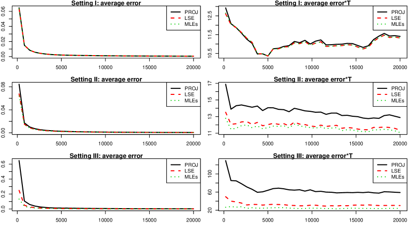
Figure 5: Comparison of the asymptotic efficiencies of three estimators, PROJ, LSE, and MLEs, under three settings. The left column shows the average error over 100 repetitions for $\|\hat{\boldsymbol{B}}\otimes\hat{\boldsymbol{A}}-{\boldsymbol{B}}\otimes{\boldsymbol{A}}\|_{F}^{2}$ and the right for $T\|\hat{\boldsymbol{B}}\otimes\hat{\boldsymbol{A}}-{\boldsymbol{B}}\otimes{\boldsymbol{A}}\|_{F}^{2}$.

In this section, we compare the performances of the aforementioned estimators and the stacked VAR(1) estimator under different settings for various choices of the matrix dimensions $m$ and $n$, as well as the length of the time series $T$.

Specifically, for given dimensions $m$ and $n$, the observed data ${\boldsymbol{X}}_{t}$ are simulated according to model (2), where the entries of ${\boldsymbol{A}}$ and ${\boldsymbol{B}}$ are generated randomly and then rescaled so that $\rho({\boldsymbol{A}})\rho({\boldsymbol{B}})=.5$ to guarantee the fulfillment of the causality condition and the constraint $||{\boldsymbol{A}}||_{F}=1$. For a particular simulation setting with multiple repetitions, the coefficient matrices ${\boldsymbol{A}}$ and ${\boldsymbol{B}}$ remain fixed.

In what follows, we perform six experiments: the first three experiments demonstrate the finite-sample comparisons under three settings of the covariance structure of the innovation matrix ${\boldsymbol{E}}_{t}$ respectively, the fourth one compares the asymptotic properties of all estimators when $T\rightarrow\infty$ under these three settings, the fifth one studies the finite-sample behavior of the asymptotic variance of the estimators, and the sixth one investigates the performance of the specification test.

• Setting I: The covariance matrix $\operatorname{Cov}(\mathrm{vec}({\boldsymbol{E}}_{t}))$ is set to $\Sigma=\mathbf{I}$.

• Setting II: The covariance matrix $\operatorname{Cov}(\mathrm{vec}({\boldsymbol{E}}_{t}))=\Sigma$ is randomly generated according to $\operatorname{Cov}(\mathrm{vec}({\boldsymbol{E}}_{t}))=\mathbf{Q}\Lambda\mathbf{Q}^{\prime}$, where the eigenvalues in the diagonal matrix $\Lambda$ are the absolute values of i.i.d. standard normal random variates, and the eigenvector matrix $\mathbf{Q}$ is a random orthonormal matrix.

• Setting III: The covariance matrix $\operatorname{Cov}(\mathrm{vec}({\boldsymbol{E}}_{t}))$ takes the Kronecker product form (4), where $\Sigma_{c}$ and $\Sigma_{r}$ are generated similarly as the $\Sigma$ in Setting II.

In addition to the three estimators (PROJ, LSE, and MLEs) discussed in Section 3, we also include the MLE under the stacked VAR(1) model in (1), with the acronym VAR, as a benchmark for comparison. For each configuration, we repeat the simulation 100 times, and show a box plot of

$$\log(\|\hat{\boldsymbol{B}}\otimes\hat{\boldsymbol{A}}-{\boldsymbol{B}}\otimes{\boldsymbol{A}}\|_{F}^{2}).$$

Figures 2 to 4 show the simulation results under three settings respectively for relatively small sample sizes. For each of these three figures, the dimensions $m,n$ increase from top to bottom, taking values in $(m,n)=(3,2),~{}(6,4)$ and $(9,6)$. The sample size $T$ increases from left to right at $T=100,200,400$ and $5000$, respectively. One common finding from these three figures is that all three estimators, PROJ, LSE, and MLEs, obtained under the MAR(1) model in (2) outperform the stacked VAR estimator.

In the first experiment under Setting I, Figure 2 shows that LSE is the best estimator when the covariance matrix is indeed a diagonal matrix. This is intuitive since LSE is the maximum likelihood estimator under this setting. The very close second best is the MLEs, which is comparable with LSE throughout different combinations of $m,~{}n,~{}T$ and only performs slightly worse when $m,~{}n$ are large and $T$ is small. This is expected since MLEs has to estimate the additional row and column covariance matrices of sizes $m\times m$ and $n\times n$ when it is not necessary. Both LSE and MLEs are superior over the PROJ, especially when the sample size is small and the dimensions are large as seen in the lower left corner of the figure. As sample size increases, the advantage becomes less obvious.

In the second experiment under Setting II, the overall pattern of Figure 3 is similar to that in Figure 2. The VAR estimator performs the worst; PROJ is the second worst, and LSE and MLEs are very much similar. Note that under Setting II, the covariance structure is arbitrary and does not follow the Kronecker structure, which is the underlying assumption for the MLEs. The LSE does not assume any covariance structure in the estimation process. Hence one would expect MLEs, obtained under the wrong assumption, should perform worse than LSE. However, the simulation results show that they perform similarly.

In the third experiment under Setting III, Figure 4 shows that MLEs dominates LSE for any choice of $m,~{}n,~{}T$, as Corollary 5 predicts. LSE in turn prevails PROJ, which in turn always leads the stacked VAR estimator.

In the fourth experiment, we compare the asymptotic efficiencies of PROJ, LSE, and MLEs by letting the length of the time series $T$ go to infinity. The main purpose of this experiment is to obtain qualitative understanding of the asymptotic covariances of different estimators. Although Theorems 2 to 4 provide the theoretical form of the asymptotic covariances and Corollary 5 ascertains the relative magnitude of the errors from LSE and MLEs under Setting III, we have little concrete insight on the relative performances of the three estimators under other settings. For this purpose, we fix the dimensions $(m,n)=(3,2)$ for all three settings in this experiment. Figure 5 shows the results. The left three panels show the average estimation errors over 100 repetitions of $\|\hat{\boldsymbol{B}}\otimes\hat{\boldsymbol{A}}-{\boldsymbol{B}}\otimes{\boldsymbol{A}}\|_{F}^{2}$ for different $T$. The right panels shows $T\|\hat{\boldsymbol{B}}\otimes\hat{\boldsymbol{A}}-{\boldsymbol{B}}\otimes{\boldsymbol{A}}\|_{F}^{2}$ as a function of $T$. The three rows correspond to the three settings respectively. In each of the six panels, the solid line, dashed line, and dotted line correspond to PROJ, LSE, and MLEs respectively. The three figures on the left show the decreasing trend of all three estimators as $T$ grows. The three figures on the right magnify the differences of the three estimators, with a clear ordering. PROJ estimator clearly has the lowest efficiency. Under Setting 1 (top panels), LSE and MLEs performs similarly, since LSE is the maximum likelihood estimators under the setting. MLEs estimates in total 4 more parameters in $\Sigma_{r}$ and $\Sigma_{c}$. The bottom panels in the figure show that MLEs is more efficient than LSE under Setting III, which is expected by Corollary 5. However, under Setting II (the middle panels), it is interesting to observe that MLEs outperforms LSE slightly but consistently, although MLEs is obtained under a wrong model assumption. This is probably due to the use of a regularized covariance structure (4), which is beneficial because of the dimension reduction from 21 parameters in an arbitrary $\Sigma$ to $8$ in $\Sigma_{c}\otimes\Sigma_{r}$. Note that the performance also depends on how close the Kronecker product approximation is to the arbitrary (random) covariance matrix used in the simulation.

In the fifth experiment, the finite-sample performance of the asymptotic covariance matrices is demonstrated. We fix the dimensions to be $m=3$ and $n=2$, and the results are similar for larger dimensions. Under each of the three aforementioned settings, combining the three estimators, PROJ, LSE, and MLEs, and their corresponding standard errors from Theorems 2 to 4, we create 95% confidence interval of each parameter based on the asymptotic normality distribution. In particular, two types of confidence intervals are constructed: one for the entries of the matrices ${\boldsymbol{A}}$ and ${\boldsymbol{B}}$ separately, and the other for the entries of $\mathrm{vec}({\boldsymbol{B}})\otimes\mathrm{vec}({\boldsymbol{A}})$. We repeat the experiment 1000 times. Table 1 shows the percentage that the true parameter falls within the marginal 95% confidence interval of each parameter for the three different estimators, under three different settings and different sample sizes. It can be seen from the table that the coverage is quite accurate, especially in large sample cases. The properties for other nominal confidence levels, for example, 90% and 99%, are similar in nature.

	Setting		I			II			III
	Estimator	PROJ	LSE	MLEs	PROJ	LSE	MLEs	PROJ	LSE	MLEs
	T=100	0.926	0.934	0.932	0.913	0.935	0.923	0.872	0.906	0.947
$(\mathrm{vec}^{\prime}(\hat{\boldsymbol{A}}),\mathrm{vec}^{\prime}(\hat{\boldsymbol{B}}))^{\prime}$	T=200	0.938	0.941	0.941	0.937	0.944	0.932	0.915	0.934	0.950
	T=1000	0.950	0.951	0.951	0.947	0.947	0.933	0.946	0.949	0.953
	T=100	0.915	0.923	0.921	0.905	0.922	0.911	0.860	0.885	0.936
$\mathrm{vec}(\hat{\boldsymbol{B}})\otimes\mathrm{vec}(\hat{\boldsymbol{A}})$	T=200	0.935	0.938	0.937	0.930	0.939	0.928	0.903	0.923	0.945
	T=1000	0.950	0.952	0.951	0.946	0.945	0.932	0.942	0.944	0.950

Table 1: Percentage of coverages of 95% confidence intervals.

In the sixth experiment, the performance of the specification test in Corollary 6 is investigated. To that end, the samples are generated according to the following models

$$\boldsymbol{X}_{t}=.5\boldsymbol{A}_{1}\boldsymbol{X}_{t-1}\boldsymbol{B}_{1}^{\prime}+.5\eta\boldsymbol{A}_{2}\boldsymbol{X}_{t-1}\boldsymbol{B}_{2}^{\prime}+\boldsymbol{E}_{t},$$

where $\rho({\boldsymbol{A}}_{1})=\rho({\boldsymbol{B}}_{1})=\rho({\boldsymbol{A}}_{2})=\rho({\boldsymbol{B}}_{2})=1,~{}\eta=0,~{}0.05,~{}0.10,~{}0.15,~{}...~{},~{}0.50$. When $\eta=0$, the null hypothesis is valid and when $\eta=0.05,~{}0.10,~{}...~{},~{}0.50$, the alternative is true. The larger the value of $\eta$ is, the more severe the deviation from the null hypothesis. Again, we fix the dimensions to be $m=3$ and $n=2$, and the results are similar for larger dimensions. The significance level is set to be 0.05 and we perform the specification test for 10,000 replications of the data with five choices of length $T$ in each of the three aforementioned settings. Figure 6 shows the empirical sizes and powers as a function of $\eta$. It can be seen that the when $\eta=0$, the empirical sizes are close to 0.05 and the powers increase to 1 as $\eta$ increases under all three settings. It is also shown that as $T$ increases, the powers increase from 0 to 1 more quickly as a function of $\eta$.

Figure 6: Power of the specification test for varying time series lengths in three settings. $\eta$ is a measure of how far the alternative hypothesis is away from the null hypothesis. The heights of the horizontal lines are 0.05.

5.2 Economic indicator from five countries

We now revisit the example shown in Figure 1. The data consists of quarterly observations of four economic indicators: 3-month interbank interest rate (first order differenced series), GDP growth (first order differenced log of GDP series), Total manufacture Production growth (first order differenced log of Production series) and total consumer price index (growth from the last period) from five countries: Canada, France, Germany, United Kingdom and United States. It ranges from 1990 to 2016. The data was obtained from Organisation for Economic Co-operation and Development (OECD) at https://data.oecd.org/. Before fitting the autoregressive models, we adjusted the seasonality of CPI by subtracting the sample quarterly means. All series are normalized so that the combined variance of each indicator (each row) is 1.

MAR(1) model was estimated using the three estimation methods. We also fitted a stacked VAR(1) model, and univariate AR(1) and AR(2) models for each individual time series. The residual sum of squares of each model and the sum of squares of the (normalized) original data are listed in Table 2. The MAR(1) estimated using the least squares method has the smallest residual sum of squares, among all models and methods, except the VAR(1) model. Note that MAR(1) model uses $16+25-1=40$ parameters in the two coefficient matrices, comparing to 20 and 40 parameters in fitting 20 univariate AR(1) and AR(2) models to each series, respectively. The VAR(1) model has total 400 parameters in the AR coefficient matrix. The large number of parameters results in a small residual sum of squares. It is deemed to be overfitting as we will show later in out-sample rolling forecasting performance evaluation.

MAR(1) PROJ	MAR(1) LSE	MAR(1) MLEs	VAR(1)	iAR(1)	iAR(2)	original
1572	1468	1487	1121	1724	1663	2116

Table 2: Residual sum of squares of MAR(1) model using three different estimators and the stacked VAR(1) estimator; and the total residual sum of squares of fitting univariate AR(1) and AR(2) to each individual time series; and the total sum of squares of the original (normalized) data.

Tables 3 and 4 show the estimated parameters and their corresponding standard errors (in the parentheses) of ${\boldsymbol{A}}$ and ${\boldsymbol{B}}$ using the least squares method. Due to ambiguity between the two matrices, the left matrix is scaled so that its Frobenius norm is one. On the right of the table we also indicate the positively significant, negatively significant and insignificant parameters (at 5% level) using symbols $(+,-,0)$, respectively.

	Int	GDP	Prod	CPI	Int	GDP	Prod	CPI
Int	0.272	0.304	0.066	0.018	$+$	$+$	$0$	$0$
	(0.063)	(0.079)	(0.097)	(0.05)
GDP	-0.164	0.447	0.32	-0.036	$-$	$+$	$+$	$0$
	(0.052)	(0.077)	(0.094)	(0.045)
Prod	-0.198	0.393	0.429	0.009	$-$	$+$	$+$	$0$
	(0.057)	(0.083)	(0.101)	(0.05)
CPI	-0.108	0.031	0.036	0.327	$0$	$0$	$0$	$+$
	(0.072)	(0.106)	(0.118)	(0.059)

Table 3: Estimated left coefficient matrix ${\boldsymbol{A}}$ of MAR(1) using LS method. Standard errors are shown in the parentheses. The right panel indicates the positively significant, negatively significant and insignificant parameters at 5% level using symbols $(+,-,0)$, respectively.

The left coefficient matrix shows an interesting pattern. For example, the first column in Table 3 shows the influence on the current economic indicators from the past quarter’s interest rate. The influence on the current GDP growth, Production growth and CPI are all negative, meaning that a higher interest rate will make the GDP growth and Production growth slower. Current CPI is also negatively related to a higher past interest rate. The second column in Table 3 shows that the influence on the current economic indicators from the past quarter’s GDP growth. They are all positive, except the insignificant influence on CPI. The last row of Table 3 shows that the past economic indicators do not have significant influence on the current CPI, except its own past; whilst the last column indicates that the past CPI does not have signifiant influence on all current indicators, except itself.

	USA	DEU	FRA	GBR	CAN	USA	DEU	FRA	GBR	CAN
USA	0.753	-0.132	0.159	0.462	-0.057	$+$	$0$	$0$	$+$	$0$
	(0.128)	(0.182)	(0.126)	(0.121)	(0.146)
DEU	0.45	0.179	0.678	0.359	-0.387	$+$	$0$	$+$	$+$	$-$
	(0.083)	(0.131)	(0.085)	(0.079)	(0.096)
FRA	0.363	0.073	0.292	0.254	0.041	$+$	$0$	$+$	$+$	$0$
	(0.128)	(0.198)	(0.139)	(0.126)	(0.154)
GBR	0.385	-0.098	0.099	0.686	0.069	$+$	$0$	$0$	$+$	$0$
	(0.115)	(0.159)	(0.109)	(0.115)	(0.132)
CAN	0.511	-0.083	0.054	0.634	0.308	$+$	$0$	$0$	$+$	$+$
	(0.098)	(0.145)	(0.1)	(0.094)	(0.115)

Table 4: Estimated right coefficient matrix ${\boldsymbol{B}}$ of MAR(1) using LS method. Standard errors are shown in parentheses. The right panel indicates the positively significant, negatively significant and insignificant parameters at 5% level using symbols $(+,-,0)$, respectively.

Table 4 shows the estimated ${\boldsymbol{B}}$. Its effect should be considered in the view of ${\boldsymbol{B}}{\boldsymbol{X}}_{t}^{\prime}$. It is seen that the influence of US’s last quarter’s indicators on the current quarter’s indicators of all countries (shown by the first column in $\hat{{\boldsymbol{B}}}$) are very significantly positive and all larger than those of all other countries. This is intuitively correct as US is the world’s largest economy. Although it is understandable that Canada has a relatively small influence on other countries (shown by the last column), it is surprising to see that Germany has almost no influence (shown by the second column). Most of the large coefficients are positive, showing positive influences among the countries. On the other hand, UK has a similar influence pattern as the US (the fourth column), a feature that is intuitively difficult to explain.

Figures 7, 8 and 9 show the shock-first impulse response functions with orthogonal innovations (s1-oIRF) with one standard deviation shock on US interest rate, US GDP and US CPI, respectively, using that given in Section 2.2. The dotted horizontal lines mark the values $(0.1,0,-0.1)$ and the dotted vertical lines marks the time $(0,2,4,6,8,10)$. It can be seen from Figure 7 that a US interest rate shock would be responded positively by the interest rates in other countries in similar patterns, and the impact lasts about a year. It is interesting to see that GDP of all countries responds positively to the interest rate shocks at first, and then negatively after two quarters, though very slightly. CPI does not have much response to interest rate shocks, but mostly in the negative direction.

From Figure 8, it is seen that the interest rate, GDP growth and Production growth of all countries respond positively to a US GDP shock, whose impacts last about 10 quarters. Again, CPI almost does not respond.

On the other hand, Figure 9 shows that a shock on US CPI generates strong positive responses from CPI of all other countries, while its impacts on interest rates, GDP growth and Production growth are also positive, but relatively small. These patterns are consistent with our interpretations on the matrix ${\boldsymbol{A}}$, reported in Table 3.

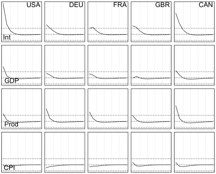
Figure 7: s1-oIRF of MAR(1) model with a unit variance shock on US interest rate.

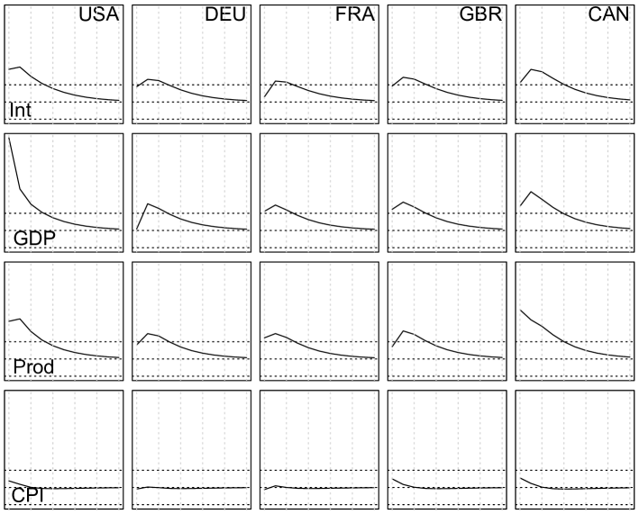
Figure 8: s1-oIRF of MAR(1) model with a unit variance shock on US GDP rate.

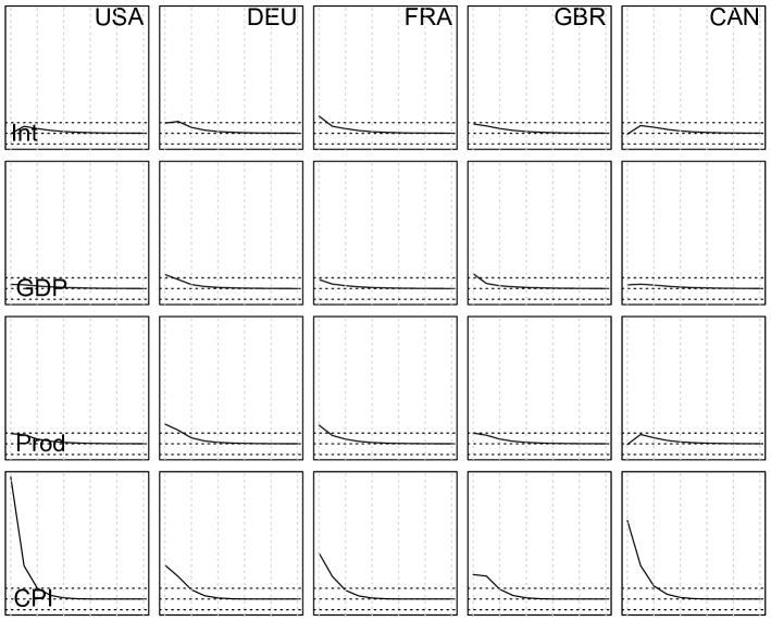
Figure 9: s1-oIRF function of MAR(1) model with a unit variance shock on US CPI rate.

Figure 10 shows the residual plots of the MAR(1) estimated using LS method. There are some outliers. Note that the analysis was done by scaling each indicator of all countries (each row) to unit sample variance. Hence the scale of the residuals (Figure 9) are different from the original data plot (Figure 1). As an illustration of the MAR(1) model, in this analysis we do not try to do any adjustment. In Figure 11 we plot the autocorrelation function (ACF) of the 20 residual series, after fitting the MAR(1) model using the least squares method. Figure 12 shows the ACF plots of the 20 original series. It is seen that the MAR(1) model is able to capture the serial correlations in the 20 time series simultaneously, and lead to relatively clean ACF plots of the residuals. Further model checking excises such as the standard portmanteau test may also be applied to assess the adequacy of the model, though more investigation needs to be done for its properties for high dimensional cases such as the model used. Note that this example is mainly for demonstration. A more thorough analysis of the data may require a model with more Kronecker production terms as in (5), or with higher AR orders.

Figure 10: Residual plot of the MAR(1) model.

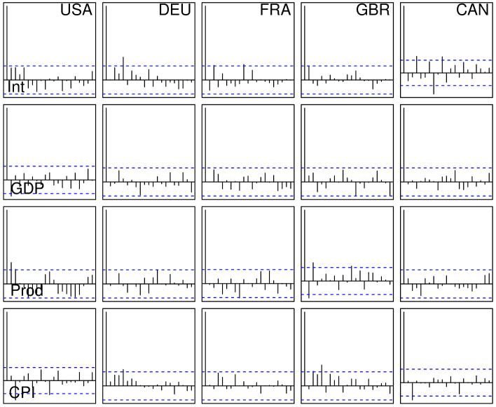
Figure 11: ACF of residuals after fitting MAR(1) model using least squares method.

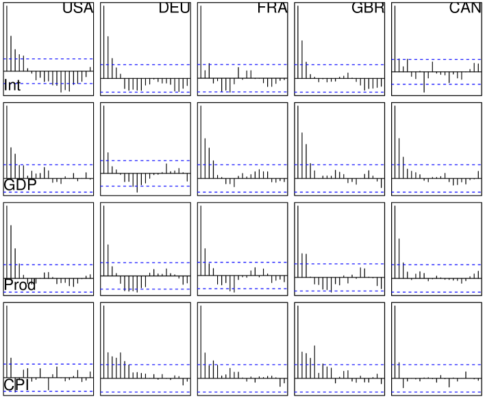
Figure 12: ACF of original series.

We also obtain out-sample rolling forecast performances of the MAR(1) model as well as univariate AR(1) and AR(2) models for comparison. Specifically, starting from the last quarter of 2011 ($t=87$) to the end of the series (the last quarter of 2016, $t=107$), we fit the corresponding models using all available data at time $t-1$ and obtained the one step ahead prediction $\hat{{\boldsymbol{X}}}_{t-1}(1)$ for ${\boldsymbol{X}}_{t}$ at time $t$. Sum of prediction error squares $||\hat{{\boldsymbol{X}}}_{t-1}(1)-{\boldsymbol{X}}_{t}||_{F}^{2}$ of all methods are shown in Table 5. It seems that MAR(1) with least squares estimation performs about 3% worse than the individual AR(1) models. It is commonly observed in multivariate time series that the joint model often performs worse than individual AR models in prediction. Figure 13 shows the difference between the sum of squares of prediction error (or all countries and all indicators) for each quarter between the MAR(1) model and the individual AR(1) model. It is seen that although MAR(1) model performs quite poorly in three out of the 20 quarters, it performs better in the later three years.

Table 5 also shows that the stacked VAR(1) model performed terribly in prediction, due to overfitting.

MAR(1) PROJ	MAR(1) LSE	MAR(1) MLEs	iAR(1)	iAR(2)	VAR(1)
146.89	141.82	136.69	136.00	135.72	296.62

Table 5: Sum of out-of-sample prediction error squares of MAR(1) model using three different estimators and the stacked VAR(1) estimator, and the total sum of out-of-sample prediction error squares of fitting univariate AR(1) and AR(2) to each individual time series.

Figure 13: The difference of the sum of prediction error squares between the MAR(1) model and individual AR(1) model at each quarter.

6 Conclusion

We proposed an autoregressive model for matrix-valued time series in a bilinear form. It respects the original matrix structure, and provides a much more parsimonious model, comparing with the direct VAR approach by stacking the matrix into a long vector. Several interpretations of the model, along with possible extensions are discussed. Different estimation methods are studied under different covariance structures of the error matrix. Asymptotic distributions of the estimators are established, which facilitate the statistical inferences.

On the other hand, when the matrix observation has large dimensions itself, our model still involves a large number of parameters, although much less than that of the corresponding stacked VAR model. Note that it is natural to have relatively large total number of parameters, due to the large number of time series involved. For example, fitting univariate AR(2) models to the $(mn)$ time series individually would require total $2mn$ AR coefficients, while MAR(1) involves $m^{2}+n^{2}-1$ AR coefficients. When $m\sim n$, they use about the same number of parameters. Also, the structured covariance (4) involves $m(m+1)/2+n(n+1)/2-1$ parameters while individual AR models involve $mn$ variance parameters, without considering any correlation among the series. Of course, regularized estimation approach can be used for MAR(1) model, potentially shrinking some of the insignificant parameters in the coefficient matrices to zero, as we have done in a rather ad hoc way in Tables 3 and 4 in the real example.

The impact of dimension $m$ and $n$ on the accuracy of the estimated parameters are hidden in the asymptotic variances of the estimators. Of course the larger the dimension, the larger the sample size $T$ is required to obtain accurate estimates. For very large dimensional matrix time series, Wang et al., (2018) proposed a factor model in a bilinear form. The MAR(1) can be used to model the factor matrix in that of Wang et al., (2018) to build a dynamic factor model in matrix form.

There are a number of directions to extend the scope of the proposed model. Sparsity, group sparsity or other structures might be imposed on ${\boldsymbol{A}}$ and ${\boldsymbol{B}}$ to reach a further dimension reduction, so that the model is better suited when both ${\boldsymbol{A}}$ and ${\boldsymbol{B}}$ are of large dimensions. We will also consider MAR models of order larger than one in the future. Furthermore, the idea of MAR can be applied for volatility modeling (Engle,, 1982; Bollerslev,, 1986) as well.

Appendix: Proofs of the Theorems

We collect the proofs of Proposition 1, Theorem 2, Theorem 3, Theorem 4, Corollary 5 and Corollary 6 in this section.

A.1 Basics

We begin by listing some basic properties of the Kronecker product and its relationship with linear matrix equations. Let $M_{m,n}$ be the set of all $m\times n$ matrices over the field of complex numbers $\mathbb{C}$. The Kronecker product of ${\boldsymbol{C}}=(c_{ij})\in M_{m,n}$, and ${\boldsymbol{D}}=(d_{ij})\in M_{p,q}$, denoted by ${\boldsymbol{C}}\otimes{\boldsymbol{D}}$, is defined to be the block matrix

$${\boldsymbol{C}}\otimes{\boldsymbol{D}}=\begin{pmatrix}c_{11}{\boldsymbol{D}}&\cdots&c_{1n}{\boldsymbol{D}}\\ \vdots&\ldots&\vdots\\ c_{m1}{\boldsymbol{D}}&\cdots&c_{mn}{\boldsymbol{D}}\end{pmatrix}\in M_{mp,nq}.$$

In the following proposition, we list some facts regarding the Kronecker product, which are used in this section at various places without specific references. Proofs of these facts can be found in Chapter 4 of Horn and Johnson, (1994).

Proposition 7.

Let ${\boldsymbol{C}}\in M_{m,n}$, ${\boldsymbol{D}}\in M_{p,q}$, ${\boldsymbol{F}}\in M_{n,k}$, ${\boldsymbol{G}}\in M_{q,l}$ and ${\boldsymbol{Z}}\in M_{n,p}$.

1. $({\boldsymbol{C}}\otimes{\boldsymbol{D}})^{\prime}={\boldsymbol{C}}^{\prime}\otimes{\boldsymbol{D}}^{\prime}$.

2. If both ${\boldsymbol{C}}$ and ${\boldsymbol{D}}$ are invertible square matrices, then ${\boldsymbol{C}}\otimes{\boldsymbol{D}}$ is also invertible, and $({\boldsymbol{C}}\otimes{\boldsymbol{D}})^{-1}={\boldsymbol{C}}^{-1}\otimes{\boldsymbol{D}}^{-1}$.

3. $({\boldsymbol{C}}\otimes{\boldsymbol{D}})({\boldsymbol{F}}\otimes{\boldsymbol{G}})=({\boldsymbol{C}}{\boldsymbol{F}})\otimes({\boldsymbol{D}}{\boldsymbol{G}})$.

4. $\mathrm{vec}({\boldsymbol{C}}{\boldsymbol{Z}}{\boldsymbol{D}})=({\boldsymbol{D}}^{\prime}\otimes{\boldsymbol{C}})\mathrm{vec}({\boldsymbol{Z}})$.

5. $\mathrm{rank}({\boldsymbol{C}}\otimes{\boldsymbol{D}})=\mathrm{rank}({\boldsymbol{D}}\otimes{\boldsymbol{C}})=\mathrm{rank}({\boldsymbol{C}})\cdot\mathrm{rank}({\boldsymbol{D}})$.

6. Let ${\boldsymbol{C}}\in M_{m,m}$ and ${\boldsymbol{D}}\in M_{n,n}$. Let $\{\lambda_{1},\lambda_{2},\ldots,\lambda_{m}\}$ be eigenvalues of ${\boldsymbol{C}}$ (including multiplicities), and $\{\eta_{1},\eta_{2},\ldots,\eta_{n}\}$ be eigenvalues of ${\boldsymbol{D}}$. The $mn$ eigenvalues (including multiplicities) of ${\boldsymbol{C}}\otimes{\boldsymbol{D}}$ are $\{\lambda_{i}\eta_{j}:\;1\leq i\leq m,\,1\leq j\leq n\}$.

Proof of Proposition 1.

It is known that the VAR(1) model in (1) admits a stationary and causal solution if the spectral radius of the coefficient matrix $\Phi$ is strictly less than 1 (See for example, §11.3 of Brockwell and Davis,, 1991). By Proposition 7$\sim$(vi), all the eigenvalues of ${\boldsymbol{B}}\otimes{\boldsymbol{A}}$ are of the form $\lambda_{i}\eta_{j}$, where $\lambda_{i}$ and $\eta_{j}$ are the eigenvalues of ${\boldsymbol{A}}$ and ${\boldsymbol{B}}$ respectively. As a consequence, $\rho({\boldsymbol{B}}\otimes{\boldsymbol{A}})=\rho({\boldsymbol{A}})\cdot\rho({\boldsymbol{B}})$. Since the MAR(1) model in (2) can be represented as a VAR model as given by (3), the proposition then follows. ∎

A.2 Proof of Theorem 2

Proof of Theorem 2.

Let ${\boldsymbol{\alpha}}=\mathrm{vec}({\boldsymbol{A}})$ and $\underline{{\boldsymbol{\beta}}}=\mathrm{vec}({\boldsymbol{B}})$. Note that the convention that $\|{\boldsymbol{A}}\|_{F}=1$ is equivalent to $\|{\boldsymbol{\alpha}}\|=1$. Also note that since ${\boldsymbol{\beta}}$ is used to denote $\mathrm{vec}({\boldsymbol{B}}^{\prime})$ in Theorem 3, we use $\underline{{\boldsymbol{\beta}}}$ here for $\mathrm{vec}({\boldsymbol{B}})$. Recall that ${\boldsymbol{\beta}}_{1}$ is the normalized version of $\underline{{\boldsymbol{\beta}}}$. The gradient condition of the NKP problem (9) is given by

$$\hat{\boldsymbol{\alpha}}\hat{}\underline{{\boldsymbol{\beta}}}^{\prime}\hat{}\underline{{\boldsymbol{\beta}}}-\tilde{\Phi}\hat{}\underline{{\boldsymbol{\beta}}} =0$$ (18)

$$\hat{}\underline{{\boldsymbol{\beta}}}\hat{\boldsymbol{\alpha}}^{\prime}\hat{\boldsymbol{\alpha}}-\tilde{\Phi}^{\prime}\hat{\boldsymbol{\alpha}} =0.$$

Recall that we require $\|\hat{\boldsymbol{A}}_{1}\|_{F}=1$, so we similarly also require that the solution of the NKP problem satisfies $\|\hat{\boldsymbol{\alpha}}\|=1$. Since both $\|{\boldsymbol{\alpha}}\|=1$ and $\|\hat{\boldsymbol{\alpha}}\|=1$ it follows that $(\hat{\boldsymbol{\alpha}}-{\boldsymbol{\alpha}})^{\prime}{\boldsymbol{\alpha}}=o_{P}(T^{-1/2})$. Replacing $\tilde{\Phi}$ by ${\boldsymbol{\alpha}}\underline{{\boldsymbol{\beta}}}^{\prime}+(\tilde{\Phi}-{\boldsymbol{\alpha}}\underline{{\boldsymbol{\beta}}}^{\prime})$ in the gradient conditions, we have

$$(\hat{\boldsymbol{\alpha}}-{\boldsymbol{\alpha}})\underline{{\boldsymbol{\beta}}}^{\prime}\underline{{\boldsymbol{\beta}}}+{\boldsymbol{\alpha}}(\hat{}\underline{{\boldsymbol{\beta}}}-\underline{{\boldsymbol{\beta}}})^{\prime}\underline{{\boldsymbol{\beta}}} =(\tilde{\Phi}-{\boldsymbol{\alpha}}\underline{{\boldsymbol{\beta}}}^{\prime})\underline{{\boldsymbol{\beta}}}+o_{P}(T^{-1/2})$$ (19)

$$\hat{}\underline{{\boldsymbol{\beta}}}-\underline{{\boldsymbol{\beta}}} =(\tilde{\Phi}-{\boldsymbol{\alpha}}\underline{{\boldsymbol{\beta}}}^{\prime})^{\prime}{\boldsymbol{\alpha}}+o_{P}(T^{-1/2}).$$

It follows that

$$\begin{pmatrix}\mathrm{vec}(\hat{\boldsymbol{A}}_{1}-{\boldsymbol{A}})\\ \mathrm{vec}(\hat{\boldsymbol{B}}_{1}-{\boldsymbol{B}})\end{pmatrix}={\boldsymbol{V}}_{0}\mathrm{vec}(\tilde{\Phi}-{\boldsymbol{\alpha}}\underline{{\boldsymbol{\beta}}}^{\prime})+o_{P}(T^{-1/2}),$$ (20)

and

$$\hat{\boldsymbol{\alpha}}\hat{}\underline{{\boldsymbol{\beta}}}^{\prime}-{\boldsymbol{\alpha}}\underline{{\boldsymbol{\beta}}}^{\prime}=(\tilde{\Phi}-{\boldsymbol{\alpha}}\underline{{\boldsymbol{\beta}}}^{\prime}){\boldsymbol{\beta}}_{1}{\boldsymbol{\beta}}_{1}^{\prime}+\alpha\alpha^{\prime}(\tilde{\Phi}-{\boldsymbol{\alpha}}\underline{{\boldsymbol{\beta}}}^{\prime})-\alpha\alpha^{\prime}(\tilde{\Phi}-{\boldsymbol{\alpha}}\underline{{\boldsymbol{\beta}}}^{\prime}){\boldsymbol{\beta}}_{1}{\boldsymbol{\beta}}_{1}^{\prime}+o_{P}(T^{-1/2}).$$ (21)

The first central limit theorem stated in Theorem 2 is an immediate consequence of (20). Taking vectorization on both sides of (21), we have

$$\hat{}\underline{{\boldsymbol{\beta}}}\otimes\hat{\boldsymbol{\alpha}}-\underline{{\boldsymbol{\beta}}}\otimes{\boldsymbol{\alpha}}={\boldsymbol{V}}_{1}\mathrm{vec}(\tilde{\Phi}-{\boldsymbol{\alpha}}\underline{{\boldsymbol{\beta}}}^{\prime})+o_{P}(T^{-1/2}),$$

and the second central limit theorem follows. ∎

A.3 Proof of Theorem 3

To prove Theorem 3, we first state and prove the following lemma.

Lemma 8.

Consider the VAR(1) representation of (3), and let $\Phi={\boldsymbol{B}}\otimes{\boldsymbol{A}}$. Assume the conditions of Theorem 3. Then for any sequence $\{c_{T}\}$ such that $c_{T}\rightarrow\infty$,

$$P\left[\inf_{\sqrt{T}\|\bar{\Phi}-\Phi\|_{F}\geq c_{T}}\sum_{t=2}^{T}\left\|\mathrm{vec}({\boldsymbol{X}}_{t})-\bar{\Phi}\mathrm{vec}({\boldsymbol{X}}_{t-1})\right\|^{2}\leq\sum_{t=2}^{T}\left\|\mathrm{vec}({\boldsymbol{E}}_{t})\right\|^{2}\right]\rightarrow 0.$$ (22)

Proof.

First of all, by the ergodic theorem

$$\frac{1}{T}\sum_{t=2}^{T}\mathrm{vec}({\boldsymbol{X}}_{t-1})\mathrm{vec}({\boldsymbol{X}}_{t-1})^{\prime}\rightarrow\Gamma_{0}\quad\hbox{a.s.}$$

It follows that for any constant $c>0$,

$$\sup_{\sqrt{T}\|\bar{\Phi}-\Phi\|_{F}\leq c} \left|\sum_{t=2}^{T}\operatorname{tr}\left[(\bar{\Phi}-\Phi)\mathrm{vec}({\boldsymbol{X}}_{t-1})\mathrm{vec}({\boldsymbol{X}}_{t-1})^{\prime}(\bar{\Phi}-\Phi)^{\prime}\right]\right.$$ (23)

$$\left.\phantom{\sum_{t=2}^{T}\!\!\!\!}-T\cdot\operatorname{tr}\left[(\bar{\Phi}-\Phi)\Gamma_{0}(\bar{\Phi}-\Phi)^{\prime}\right]\right|\rightarrow 0\quad\hbox{a.s.}$$

In (23), the superme is taken over $\bar{\Phi}$. As a consequence of (23), there exists a sequence $\{c_{T}^{\prime}\}$ such that $c_{T}^{\prime}\rightarrow\infty$, $c_{T}^{\prime}\leq c_{T}$, and

$$\sup_{\sqrt{T}\|\bar{\Phi}-\Phi\|_{F}\leq c_{T}^{\prime}} \left|\sum_{t=2}^{T}\operatorname{tr}\left[(\bar{\Phi}-\Phi)\mathrm{vec}({\boldsymbol{X}}_{t-1})\mathrm{vec}({\boldsymbol{X}}_{t-1})^{\prime}(\bar{\Phi}-\Phi)^{\prime}\right]\right.$$ (24)

$$\left.\phantom{\sum_{t=2}^{T}\!\!\!\!}-T\cdot\operatorname{tr}\left[(\bar{\Phi}-\Phi)\Gamma_{0}(\bar{\Phi}-\Phi)^{\prime}\right]\right|\rightarrow 0\quad\hbox{in probability}.$$

Now we write

$$\sum_{t=2}^{T}\left\|\mathrm{vec}({\boldsymbol{X}}_{t})-\bar{\Phi}\mathrm{vec}({\boldsymbol{X}}_{t-1})\right\|^{2}-\sum_{t=2}^{T}\left\|\mathrm{vec}({\boldsymbol{E}}_{t})\right\|^{2}$$ (25)

$$= -2\sum_{t=2}^{T}\operatorname{tr}\left[(\bar{\Phi}-\Phi)\mathrm{vec}({\boldsymbol{X}}_{t-1})\mathrm{vec}({\boldsymbol{E}}_{t})^{\prime}\right]+\sum_{t=2}^{T}\operatorname{tr}\left[(\bar{\Phi}-\Phi)\mathrm{vec}({\boldsymbol{X}}_{t-1})\mathrm{vec}({\boldsymbol{X}}_{t-1})^{\prime}(\bar{\Phi}-\Phi)^{\prime}\right].$$

On the boundary set $\sqrt{T}\|\bar{\Phi}-\Phi\|_{F}=c_{T}^{\prime}$, by calculating the variance, we know that

$$\sum_{t=2}^{T}\operatorname{tr}\left[(\bar{\Phi}-\Phi)\mathrm{vec}({\boldsymbol{X}}_{t-1})\mathrm{vec}({\boldsymbol{E}}_{t})^{\prime}\right]=O_{P}(c_{T}^{\prime}).$$ (26)

On the other hand, on the boundary set $\sqrt{T}\|\bar{\Phi}-\Phi\|_{F}=c_{T}^{\prime}$,

$$T\cdot\operatorname{tr}\left[(\bar{\Phi}-\Phi)\Gamma_{0}(\bar{\Phi}-\Phi)^{\prime}\right]\geq{\lambda_{\min}}(\Gamma_{0})(c_{T}^{\prime})^{2},$$ (27)

where ${\lambda_{\min}}(\Gamma_{0})$ is the minimum eigenvalue of $\Gamma_{0}$, which is strictly positive under the condition that ${\boldsymbol{A}}$, ${\boldsymbol{B}}$ and $\Sigma$ are nonsingular. Combining (24)$\sim$(27), and with fact that $c_{T}^{\prime}\rightarrow\infty$, we have

$$P\left[\inf_{\sqrt{T}\|\bar{\Phi}-\Phi\|_{F}=c_{T}^{\prime}}\sum_{t=2}^{T}\left\|\mathrm{vec}({\boldsymbol{X}}_{t})-\bar{\Phi}\mathrm{vec}({\boldsymbol{X}}_{t-1})\right\|^{2}\leq\sum_{t=2}^{T}\left\|\mathrm{vec}({\boldsymbol{E}}_{t})\right\|^{2}\right]\rightarrow 0.$$ (28)

Observe that $\sum_{t=2}^{T}\left\|\mathrm{vec}({\boldsymbol{X}}_{t})-\bar{\Phi}\mathrm{vec}({\boldsymbol{X}}_{t-1})\right\|^{2}$ is a convex function of $\bar{\Phi}$, so (22) is implied by (28) and the convexity. ∎

Now we are ready to give the proof of Theorem 3.

Proof of Theorem 3.

Let $\mathbb{S}=\{{\boldsymbol{C}}:\,{\boldsymbol{C}}\hbox{ is a }m\times m\hbox{ matrix, and }\|{\boldsymbol{C}}\|_{F}=1\}$. Let $\{c_{T}\}$ be any sequence such that $c_{T}\rightarrow\infty$, and $c_{T}/\sqrt{T}\rightarrow 0$. By the conditions that ${\boldsymbol{A}}$ and ${\boldsymbol{B}}$ are nonsingular, and ${\boldsymbol{A}}\in\mathbb{S}$, it can be show that if $\bar{\boldsymbol{A}}$ and $\bar{\boldsymbol{B}}$ are such that $\bar{\boldsymbol{A}}\in\mathbb{S}$, and $T\|\bar{\boldsymbol{A}}-{\boldsymbol{A}}\|_{F}^{2}+T\|\bar{\boldsymbol{B}}-{\boldsymbol{B}}\|_{F}^{2}\geq c_{T}^{2}$, then $\|\bar{\boldsymbol{B}}\otimes\bar{\boldsymbol{A}}-{\boldsymbol{B}}\otimes{\boldsymbol{A}}\|_{F}\geq C\cdot c_{T}$, where $C$ is a constant determined by ${\boldsymbol{A}}$ and ${\boldsymbol{B}}$. By Lemma 8, we have

$$P\left[\min_{T\|\bar{\boldsymbol{A}}-{\boldsymbol{A}}\|_{F}^{2}+T\|\bar{\boldsymbol{B}}-{\boldsymbol{B}}\|_{F}^{2}\geq c_{T}^{2}}\sum_{t=2}^{T}\left\|\mathrm{vec}({\boldsymbol{X}}_{t})-(\bar{\boldsymbol{B}}\otimes\bar{\boldsymbol{A}})\mathrm{vec}({\boldsymbol{X}}_{t-1})\right\|^{2}\leq\sum_{t=2}^{T}\left\|\mathrm{vec}({\boldsymbol{E}}_{t})\right\|^{2}\right]\rightarrow 0,$$

with the implicit requirement that $\bar{\boldsymbol{A}}\in\mathbb{S}$. It follows that

$$P\left[T\|\hat{\boldsymbol{A}}-{\boldsymbol{A}}\|_{F}^{2}+T\|\hat{\boldsymbol{B}}-{\boldsymbol{B}}\|_{F}^{2}\leq c_{T}^{2}\right]\rightarrow 1,$$ (29)

also with the implicit requirement that $\hat{\boldsymbol{A}}\in\mathbb{S}$. Since (29) holds for any sequence $\{c_{T}\}$ such that $c_{T}\rightarrow\infty$, and $c_{T}/\sqrt{T}\rightarrow 0$, we have

$$\hat{\boldsymbol{A}}={\boldsymbol{A}}+O_{P}(T^{-1/2}),\quad\hbox{and}\quad\hat{\boldsymbol{B}}={\boldsymbol{B}}+O_{P}(T^{-1/2}).$$

We now repeat the gradient condition (15) here:

$$\sum_{t}\hat{\boldsymbol{A}}_{2}{\boldsymbol{X}}_{t-1}\hat{\boldsymbol{B}}_{2}^{\prime}\hat{\boldsymbol{B}}_{2}{\boldsymbol{X}}_{t-1}^{\prime}-\sum_{t}{\boldsymbol{X}}_{t}\hat{\boldsymbol{B}}_{2}{\boldsymbol{X}}_{t-1}^{\prime} ={\boldsymbol{0}}$$ (30)

$$\sum_{t}\hat{\boldsymbol{B}}_{2}{\boldsymbol{X}}_{t-1}^{\prime}\hat{\boldsymbol{A}}_{2}^{\prime}\hat{\boldsymbol{A}}_{2}{\boldsymbol{X}}_{t-1}-\sum_{t}{\boldsymbol{X}}_{t}^{\prime}\hat{\boldsymbol{A}}_{2}{\boldsymbol{X}}_{t-1} ={\boldsymbol{0}}.$$

Replacing each ${\boldsymbol{X}}_{t}$ by ${\boldsymbol{A}}{\boldsymbol{X}}_{t-1}{\boldsymbol{B}}^{\prime}+{\boldsymbol{E}}_{t}$ in (30), we have

$$\sum_{t}(\hat{\boldsymbol{A}}_{2}-{\boldsymbol{A}}){\boldsymbol{X}}_{t-1}{\boldsymbol{B}}^{\prime}{\boldsymbol{B}}{\boldsymbol{X}}_{t-1}^{\prime}+\sum_{t}{\boldsymbol{A}}{\boldsymbol{X}}_{t-1}(\hat{\boldsymbol{B}}_{2}-{\boldsymbol{B}})^{\prime}{\boldsymbol{B}}{\boldsymbol{X}}_{t-1}^{\prime} =\sum_{t}{\boldsymbol{E}}_{t}{\boldsymbol{B}}{\boldsymbol{X}}_{t-1}^{\prime}+o_{P}(\sqrt{T})$$

$$\sum_{t}{\boldsymbol{X}}_{t-1}^{\prime}{\boldsymbol{A}}^{\prime}(\hat{\boldsymbol{A}}_{2}-{\boldsymbol{A}}){\boldsymbol{X}}_{t-1}{\boldsymbol{B}}^{\prime}+\sum_{t}{\boldsymbol{X}}_{t-1}^{\prime}{\boldsymbol{A}}^{\prime}{\boldsymbol{A}}{\boldsymbol{X}}_{t-1}(\hat{\boldsymbol{B}}_{2}-{\boldsymbol{B}})^{\prime} =\sum_{t}{\boldsymbol{X}}_{t-1}^{\prime}{\boldsymbol{A}}^{\prime}{\boldsymbol{E}}_{t}+o_{P}(\sqrt{T}).$$

Taking vectorization on both sides, we have

$$\begin{pmatrix}\left(\sum_{t}{\boldsymbol{X}}_{t-1}{\boldsymbol{B}}^{\prime}{\boldsymbol{B}}{\boldsymbol{X}}_{t-1}^{\prime}\right)\otimes{\boldsymbol{I}}&\sum_{t}({\boldsymbol{X}}_{t-1}{\boldsymbol{B}}^{\prime})\otimes({\boldsymbol{A}}{\boldsymbol{X}}_{t-1})\\ \sum_{t}({\boldsymbol{B}}{\boldsymbol{X}}_{t-1}^{\prime})\otimes({\boldsymbol{X}}_{t-1}^{\prime}{\boldsymbol{A}}^{\prime})&{\boldsymbol{I}}\otimes\left(\sum_{t}{\boldsymbol{X}}_{t-1}^{\prime}{\boldsymbol{A}}^{\prime}{\boldsymbol{A}}{\boldsymbol{X}}_{t-1}\right)\end{pmatrix}\begin{pmatrix}\mathrm{vec}(\hat{\boldsymbol{A}}_{2}-{\boldsymbol{A}})\\ \mathrm{vec}(\hat{\boldsymbol{B}}_{2}^{\prime}-{\boldsymbol{B}}^{\prime})\end{pmatrix}$$

$$= \sum_{t}\begin{pmatrix}({\boldsymbol{X}}_{t-1}{\boldsymbol{B}}^{\prime})\otimes{\boldsymbol{I}}\\ {\boldsymbol{I}}\otimes({\boldsymbol{X}}_{t-1}^{\prime}{\boldsymbol{A}}^{\prime})\end{pmatrix}\mathrm{vec}({\boldsymbol{E}}_{t})+o_{P}(\sqrt{T}),$$

which can be rewritten as

$$\left(\sum_{t}{\boldsymbol{W}}_{t-1}{\boldsymbol{W}}_{t-1}^{\prime}\right)\begin{pmatrix}\mathrm{vec}(\hat{\boldsymbol{A}}_{2}-{\boldsymbol{A}})\\ \mathrm{vec}(\hat{\boldsymbol{B}}_{2}^{\prime}-{\boldsymbol{B}}^{\prime})\end{pmatrix}=\sum_{t}{\boldsymbol{W}}_{t-1}\mathrm{vec}({\boldsymbol{E}}_{t})+o_{P}(\sqrt{T}).$$ (31)

By the ergodic theorem as ${\boldsymbol{X}}_{t}$ is strictly stationary with i.i.d. innovations under the conditions, we have

$$\frac{1}{T}\sum_{t}{\boldsymbol{W}}_{t-1}{\boldsymbol{W}}_{t-1}^{\prime}\rightarrow\mathbb{E}({\boldsymbol{W}}_{t}{\boldsymbol{W}}_{t}^{\prime}),\quad\hbox{a.s.}$$

Observe that $\mathbb{E}({\boldsymbol{W}}_{t}{\boldsymbol{W}}_{t}^{\prime})$ is not a full rank matrix, because $\mathbb{E}({\boldsymbol{W}}_{t}{\boldsymbol{W}}_{t}^{\prime})({\boldsymbol{\alpha}}^{\prime},-{\boldsymbol{\beta}}^{\prime})^{\prime}={\boldsymbol{0}}$. On the other hand, since we require $\|{\boldsymbol{A}}\|_{F}=1$ and $\|\hat{\boldsymbol{A}}_{2}\|_{F}=1$, it holds that ${\boldsymbol{\alpha}}^{\prime}(\mathrm{vec}(\hat{\boldsymbol{A}}_{2})-{\boldsymbol{\alpha}})=o_{P}(T^{-1/2})$. and consequently

$${\boldsymbol{H}}\begin{pmatrix}\mathrm{vec}(\hat{\boldsymbol{A}}_{2}-{\boldsymbol{A}})\\ \mathrm{vec}(\hat{\boldsymbol{B}}_{2}^{\prime}-{\boldsymbol{B}}^{\prime})\end{pmatrix}=\frac{1}{T}\sum_{t}{\boldsymbol{W}}_{t-1}\mathrm{vec}({\boldsymbol{E}}_{t})+o_{P}(T^{-1/2}),$$

where ${\boldsymbol{H}}:=\mathbb{E}({\boldsymbol{W}}_{t}{\boldsymbol{W}}_{t}^{\prime})+{\boldsymbol{\gamma}}{\boldsymbol{\gamma}}^{\prime}$. By martingale central limit theorem (Hall and Heyde,, 1980)

$$\sum_{t}{\boldsymbol{W}}_{t-1}\mathrm{vec}({\boldsymbol{E}}_{t})\Rightarrow N({\boldsymbol{0}},\mathbb{E}({\boldsymbol{W}}_{t}\Sigma{\boldsymbol{W}}_{t}^{\prime})).$$

It follows that

$$\sqrt{T}\begin{pmatrix}\mathrm{vec}(\hat{\boldsymbol{A}}_{2}-{\boldsymbol{A}})\\ \mathrm{vec}(\hat{\boldsymbol{B}}_{2}^{\prime}-{\boldsymbol{B}}^{\prime})\end{pmatrix}\Rightarrow N({\boldsymbol{0}},\Xi_{2}),$$

where $\Xi_{2}:={\boldsymbol{H}}^{-1}\mathbb{E}({\boldsymbol{W}}_{t}\Sigma{\boldsymbol{W}}_{t}^{\prime}){\boldsymbol{H}}^{-1}$. Furthermore, noting that

$$\mathrm{vec}(\hat{{\boldsymbol{B}}}_{2}^{\prime})\otimes\mathrm{vec}(\hat{{\boldsymbol{A}}}_{2})-\mathrm{vec}({\boldsymbol{B}}^{\prime})\otimes\mathrm{vec}({\boldsymbol{A}})$$

$$= \mathrm{vec}(\hat{\boldsymbol{B}}_{2}^{\prime}-{\boldsymbol{B}}^{\prime})\otimes{\boldsymbol{\alpha}}+{\boldsymbol{\beta}}\otimes\mathrm{vec}(\hat{\boldsymbol{A}}_{2}-{\boldsymbol{A}})$$

$$= {\boldsymbol{V}}\begin{pmatrix}\mathrm{vec}(\hat{\boldsymbol{A}}_{2}-{\boldsymbol{A}})\\ \mathrm{vec}(\hat{\boldsymbol{B}}_{2}^{\prime}-{\boldsymbol{B}}^{\prime})\end{pmatrix}+o_{P}(T^{-1/2}),$$

where ${\boldsymbol{V}}:=[{\boldsymbol{\beta}}\otimes{\boldsymbol{I}},{\boldsymbol{I}}\otimes{\boldsymbol{\alpha}}]$, the statement about ${\boldsymbol{B}}\otimes{\boldsymbol{A}}$ in the theorem follows. The proof is complete. ∎

A.4 Proof of Theorem 4

To prove Theorem 4, we first list some properties of the function:

$$h(\Omega,{\boldsymbol{S}})=-\log|\Omega|+\operatorname{tr}(\Omega{\boldsymbol{S}}),$$ (32)

where both $\Omega$ and ${\boldsymbol{S}}$ are positive definite matrices. The first property is adapted from Theorem 7.6.6 of Horn and Johnson, (2012); and the second one can be proved by straightforward arguments, so we skip the proof.

Proposition 9.

Assume both $\Omega$ and ${\boldsymbol{S}}$ are positive definite matrices of the same dimension.

1. Fix ${\boldsymbol{S}}$, the function $h(\Omega,{\boldsymbol{S}})$ is convex in $\Omega$ over the cone of positive definite matrices.

2. Fix ${\boldsymbol{S}}$, the second order Taylor expansion of $h(\Omega,{\boldsymbol{S}})$ around $\Omega$ is given by

   $$h(\bar{\Omega},{\boldsymbol{S}})\approx h(\Omega,{\boldsymbol{S}})-\operatorname{tr}\left[(\Omega^{-1}-{\boldsymbol{S}})(\bar{\Omega}-\Omega)\right]+\tfrac{1}{2}[\mathrm{vec}(\bar{\Omega}-\Omega)]^{\prime}(\Omega^{-1}\otimes\Omega^{-1})\mathrm{vec}(\bar{\Omega}-\Omega).$$

Proof of Theorem 4.

To avoid the unidentifiability regarding $\Sigma_{r}$ and $\Sigma_{c}$, we make the convention that $\|\Sigma_{r}\|_{F}=1$. We will only prove that $\hat{\boldsymbol{A}}_{3}={\boldsymbol{A}}+O_{P}(T^{-1/2})$, $\hat{\boldsymbol{B}}_{3}={\boldsymbol{B}}+O_{P}(T^{-1/2})$, $\hat{\Sigma}_{c}=\Sigma_{c}+o_{P}(1)$, and $\hat{\Sigma}_{r}=\Sigma_{r}+o_{P}(1)$; and omit the rest of the proof, which is very similar with that of Theorem 3.

We first set up the notations for the proof. The matrices ${\boldsymbol{A}}$, ${\boldsymbol{B}}$, $\Phi:={\boldsymbol{B}}\otimes{\boldsymbol{A}}$, $\Sigma_{r}$, $\Sigma_{c}$ and $\Sigma:=\Sigma_{c}\otimes\Sigma_{r}$ are used for the true parameters. We use $\hat{\boldsymbol{A}}_{3}$, $\hat{\boldsymbol{B}}_{3}$, $\hat{\Phi}_{3}=\hat{\boldsymbol{B}}_{3}\otimes\hat{\boldsymbol{A}}_{3}$, $\hat{\Sigma}_{r}$, $\hat{\Sigma}_{c}$, and $\hat{\Sigma}=\hat{\Sigma}_{c}\otimes\hat{\Sigma}_{r}$ to denote the MLE under (17). By the invariance property of MLE, finding the MLE of the covariance matrix $\Sigma=\Sigma_{c}\otimes\Sigma_{r}$ is equivalent as finding the MLE of the precision matrix $\Omega:=\Sigma^{-1}=\Omega_{c}\otimes\Omega_{r}$, where $\Omega_{r}=\Sigma_{r}^{-1}$ and $\Omega_{c}=\Sigma_{c}^{-1}$. Again $\hat{\Omega}$, $\hat{\Omega}_{r}$ and $\hat{\Omega}_{c}$ will denote the corresponding MLE under (17). Recall the definition of $\boldsymbol{\mathcal{X}}$ and $\boldsymbol{\mathcal{Y}}$ in (11). For the unrestriced VAR(1) model (1) for $\mathrm{vec}({\boldsymbol{X}}_{t})$, its log likelihood at the parameters $(\bar{\Phi},\bar{\Sigma})$, is

$$\ell(\bar{\Phi},\bar{\Sigma})=-\tfrac{T-1}{2}\cdot h(\bar{\Omega},{\boldsymbol{S}}(\bar{\Phi})),$$ (33)

where $\bar{\Omega}:=\bar{\Sigma}^{-1}$, and ${\boldsymbol{S}}(\bar{\Phi}):=(\boldsymbol{\mathcal{Y}}-\bar{\Phi}\boldsymbol{\mathcal{X}})(\boldsymbol{\mathcal{Y}}-\bar{\Phi}\boldsymbol{\mathcal{X}})^{\prime}/(T-1)$. Let $\check{\Phi}:=\boldsymbol{\mathcal{Y}}\boldsymbol{\mathcal{X}}^{\prime}(\boldsymbol{\mathcal{X}}\boldsymbol{\mathcal{X}}^{\prime})^{-1}$, and $\check{\boldsymbol{S}}:={\boldsymbol{S}}(\check{\Phi})=(\boldsymbol{\mathcal{Y}}-\check{\Phi}\boldsymbol{\mathcal{X}})(\boldsymbol{\mathcal{Y}}-\check{\Phi}\boldsymbol{\mathcal{X}})^{\prime}/(T-1)$. Note that $\hat{\Phi}$ and $\hat{\boldsymbol{S}}$ are MLE for the unrestricted VAR(1) model (1).

For a given $\bar{\Omega}$, the function $h(\bar{\Omega},\bar{\boldsymbol{S}})$ is minimized at $\bar{\boldsymbol{S}}=\check{\boldsymbol{S}}$, with the minimum value $h(\bar{\Omega},\check{\boldsymbol{S}})$. Let $\check{\Omega}:=\check{\boldsymbol{S}}^{-1}$ be the MLE of $\Omega$ under (1). We now prove that for any constant $c>0$

$$P\left[\inf_{\|\bar{\Omega}-\Omega\|_{F}\geq c}h(\bar{\Omega},\check{\boldsymbol{S}})\leq h(\Omega,{\boldsymbol{S}}(\Phi))\right]\rightarrow 0,$$ (34)

which implies that $\hat{\Sigma}_{c}$ and $\hat{\Sigma}_{r}$ are consistent for $\Sigma_{c}$ and $\Sigma_{r}$.

By Proposition 9, the multivariate Taylor expansion of the function $h(\bar{\Omega},\check{\boldsymbol{S}})$ around $\check{\Omega}$ gives

$$h(\bar{\Omega},\check{\boldsymbol{S}})=h(\check{\Omega},\check{\boldsymbol{S}})+\tfrac{1}{2}[\mathrm{vec}(\bar{\Omega}-\check{\Omega})]^{\prime}(\tilde{\Omega}^{-1}\otimes\tilde{\Omega}^{-1})\mathrm{vec}(\bar{\Omega}-\check{\Omega}),$$

where $\tilde{\Omega}=\check{\Omega}+\theta(\bar{\Omega}-\check{\Omega})$ for some $0<\theta<1$. By the ergodic theorem, ${\boldsymbol{S}}(\Phi)\stackrel{{\scriptstyle\hbox{\footnotesize a.s.}}}{{\longrightarrow}}\Sigma$, and $\check{\boldsymbol{S}}\stackrel{{\scriptstyle\hbox{\footnotesize a.s.}}}{{\longrightarrow}}\Sigma$, and consequently $\check{\Omega}\stackrel{{\scriptstyle\hbox{\footnotesize a.s.}}}{{\longrightarrow}}\Omega$. It follows that for any $c>0$ that is small enough, both the following two events hold with probability approaching one:

$$[\|\bar{\Omega}-\check{\Omega}\|\geq c/2\hbox{ for all }\bar{\Omega}\hbox{ on the circle }\|\bar{\Omega}-\Omega\|_{F}=c],$$

$$[\lambda_{\min}(\tilde{\Omega}^{-1}\otimes\tilde{\Omega}^{-1})>\tfrac{1}{2}\lambda_{\min}^{2}(\Omega^{-1})\hbox{ for all }\bar{\Omega}\hbox{ on the circle }\|\bar{\Omega}-\Omega\|_{F}=c],$$

where $\lambda_{\min}(\cdot)$ denotes the minimum eigenvalue of a symmetric matrix. On the intersection of these two events,

$$\tfrac{1}{2}\mathrm{vec}(\bar{\Omega}-\check{\Omega})(\tilde{\Omega}^{-1}\otimes\tilde{\Omega}^{-1})[\mathrm{vec}(\bar{\Omega}-\check{\Omega})]^{\prime}\geq\tfrac{1}{16}\lambda_{\min}^{2}(\Omega^{-1})\cdot c^{2}.$$

Since $h(\Omega,{\boldsymbol{S}}(\Phi))\stackrel{{\scriptstyle\hbox{\footnotesize a.s.}}}{{\longrightarrow}}h(\Omega,\Sigma)$ and $h(\check{\Omega},\check{\boldsymbol{S}})\stackrel{{\scriptstyle\hbox{\footnotesize a.s.}}}{{\longrightarrow}}h(\Omega,\Sigma)$, it follows that for any $c>0$ that is small enough

$$P\left[\sup_{\|\bar{\Omega}-\Omega\|_{F}=c}h(\bar{\Omega},\check{\boldsymbol{S}})\leq h(\Omega,{\boldsymbol{S}}(\Phi))\right]\rightarrow 0.$$

Therefore, (34) holds by the convexity of $h(\bar{\Omega},\check{\boldsymbol{S}})$, when viewed as a function of $\bar{\Omega}$ (see Proposition 9).

We now prove that $\hat{\boldsymbol{A}}_{3}={\boldsymbol{A}}+O_{P}(T^{-1/2})$, and $\hat{\boldsymbol{B}}_{3}={\boldsymbol{B}}+O_{P}(T^{-1/2})$. Define the set $\mathcal{H}$ to be the collection of all positive definite matrices of the Kronecker product form:

$$\mathcal{H}=\{\bar{\Omega}:\;\bar{\Omega}=\bar{\Omega}_{c}\otimes\bar{\Omega}_{r}\hbox{ for some $m\times m$ and $n\times n$ positive definite matrices }\bar{\Omega}_{r}\hbox{ and }\bar{\Omega}_{c}\}.$$

It suffices to show that for any seuqnce $c_{T}\rightarrow\infty$,

$$P\left[\inf_{\sqrt{T}\|\bar{\Phi}-\Phi\|_{F}\geq c_{T}}\inf_{\bar{\Omega}\in\mathcal{H}}h(\bar{\Omega},{\boldsymbol{S}}(\bar{\Phi}))\leq\inf_{\bar{\Omega}\in\mathcal{H}}h(\bar{\Omega},{\boldsymbol{S}}(\Phi))\right]\rightarrow 0.$$ (35)

Note that for any $\bar{\Phi}$,

$$(\boldsymbol{\mathcal{Y}}-\bar{\Phi}\boldsymbol{\mathcal{X}})(\boldsymbol{\mathcal{Y}}-\bar{\Phi}\boldsymbol{\mathcal{X}})^{\prime}=(\boldsymbol{\mathcal{Y}}-\check{\Phi}\boldsymbol{\mathcal{X}})(\boldsymbol{\mathcal{Y}}-\check{\Phi}\boldsymbol{\mathcal{X}})^{\prime}+(\bar{\Phi}-\hat{\Phi})\boldsymbol{\mathcal{X}}\boldsymbol{\mathcal{X}}^{\prime}(\bar{\Phi}-\check{\Phi})^{\prime}.$$

Let $\hat{\Gamma}_{0}:=\boldsymbol{\mathcal{X}}\boldsymbol{\mathcal{X}}^{\prime}/(T-1)$ be the sample covariance matrix of $\mathrm{vec}({\boldsymbol{X}}_{t})$, then the preceding equation can be written in the compact form

$${\boldsymbol{S}}(\bar{\Phi})=\check{\boldsymbol{S}}+(\bar{\Phi}-\hat{\Phi})\hat{\Gamma}_{0}(\bar{\Phi}-\check{\Phi})^{\prime},$$

which leads to

$$h[\bar{\Omega},{\boldsymbol{S}}(\bar{\Phi})] =h(\bar{\Omega},\check{\boldsymbol{S}})+\operatorname{tr}[\bar{\Omega}(\bar{\Phi}-\hat{\Phi})\hat{\Gamma}_{0}(\bar{\Phi}-\check{\Phi})^{\prime}]$$

$$\geq h(\bar{\Omega},\check{\boldsymbol{S}})+\lambda_{\min}(\bar{\Omega})\cdot\lambda_{\min}(\hat{\Gamma}_{0})\cdot\|\bar{\Phi}-\check{\Phi}\|_{F}^{2}.$$

According to (34), for any constant $c>0$, the following event holds with probability tending to 1:

$$\left[\inf_{\|\bar{\Omega}-\Omega\|_{F}\geq c}h(\bar{\Omega},\check{\boldsymbol{S}})>h(\Omega,{\boldsymbol{S}}(\Phi))\geq\inf_{\bar{\Omega}\in\mathcal{H}}h(\bar{\Omega},{\boldsymbol{S}}(\Phi))\right].$$ (36)

On the other hand, there exists a constant $C_{1}>0$, such that

$$\inf_{\{\bar{\Omega}\in\mathcal{H}:\,\|\bar{\Omega}-\Omega\|_{F}\leq C_{1}\}}\lambda_{\min}(\bar{\Omega})\geq\tfrac{1}{2}\lambda_{\min}(\Omega).$$

It follows that

$$\inf_{\{\bar{\Omega}\in\mathcal{H}:\,\|\bar{\Omega}-\Omega\|_{F}\leq C_{1}\}}h[\bar{\Omega},{\boldsymbol{S}}(\bar{\Phi})]\geq\inf_{\{\bar{\Omega}\in\mathcal{H}:\,\|\bar{\Omega}-\Omega\|_{F}\leq C_{1}\}}h[\bar{\Omega},\check{\boldsymbol{S}}]+\tfrac{1}{2}\lambda_{\min}(\Omega)\cdot\lambda_{\min}(\hat{\Gamma}_{0})\cdot\|\bar{\Phi}-\check{\Phi}\|_{F}^{2}.$$ (37)

Since $\hat{\Gamma}_{0}\stackrel{{\scriptstyle\hbox{\footnotesize a.s.}}}{{\longrightarrow}}\Gamma_{0}$ and $\check{\Phi}=\Phi+O_{P}(1/\sqrt{T})$, we know

$$P\left[\inf_{\sqrt{T}\|\bar{\Phi}-\Phi\|_{F}\geq c_{T}}\lambda_{\min}(\hat{\Gamma}_{0})\cdot\|\bar{\Phi}-\check{\Phi}\|_{F}^{2}\geq\tfrac{1}{2}\lambda_{\min}(\Gamma_{0})\cdot c_{T}^{2}/T\right]\rightarrow 1.$$ (38)

Consider the function $h(\bar{\Omega},{\boldsymbol{S}}(\Phi))$. Since

$${\boldsymbol{S}}(\Phi)=\check{\boldsymbol{S}}+(\Phi-\hat{\Phi})\hat{\Gamma}_{0}(\Phi-\check{\Phi})^{\prime},$$

it holds that

$$\inf_{\{\bar{\Omega}\in\mathcal{H}:\,\|\bar{\Omega}-\Omega\|_{F}\leq C_{1}\}}h[\bar{\Omega},{\boldsymbol{S}}(\Phi)] =\inf_{\{\bar{\Omega}\in\mathcal{H}:\,\|\bar{\Omega}-\Omega\|_{F}\leq C_{1}\}}\left\{h(\bar{\Omega},\check{\boldsymbol{S}})+\operatorname{tr}[\bar{\Omega}(\Phi-\check{\Phi})\hat{\Gamma}_{0}(\Phi-\check{\Phi})^{\prime}]\right\}$$ (39)

$$=\inf_{\{\bar{\Omega}\in\mathcal{H}:\,\|\bar{\Omega}-\Omega\|_{F}\leq C_{1}\}}h(\bar{\Omega},\check{\boldsymbol{S}})+O_{P}(T^{-1}).$$

Combining (37) (38) and (39), and noting that $c_{T}\rightarrow\infty$, we have established that with probability converging to 1,

$$\inf_{\sqrt{T}\|\bar{\Phi}-\Phi\|_{F}\geq c_{T}}\inf_{\{\bar{\Omega}\in\mathcal{H}:\,\|\bar{\Omega}-\Omega\|_{F}\leq C_{1}\}}h[\bar{\Omega},{\boldsymbol{S}}(\bar{\Phi})]>\inf_{\{\bar{\Omega}\in\mathcal{H}:\,\|\bar{\Omega}-\Omega\|_{F}\leq C_{1}\}}h[\bar{\Omega},{\boldsymbol{S}}(\Phi)].$$

The preceding equation, together with (36), implies (35); and the proof is therefore complete. ∎

A.5 Proof of Corollaries

Proof of Corollary 5.

From Theorem 3 and Theorem 4, we have

$$\Xi_{2} =[\mathbb{E}({\boldsymbol{W}}_{t}{\boldsymbol{W}}_{t}^{\prime})+{\boldsymbol{\gamma}}{\boldsymbol{\gamma}}^{\prime}]^{-1}\mathbb{E}({\boldsymbol{W}}_{t}\Sigma{\boldsymbol{W}}_{t}^{\prime})[\mathbb{E}({\boldsymbol{W}}_{t}{\boldsymbol{W}}_{t}^{\prime})+{\boldsymbol{\gamma}}{\boldsymbol{\gamma}}^{\prime}]^{-1},$$

$$\Xi_{3} =[\mathbb{E}({\boldsymbol{W}}_{t}\Sigma^{-1}{\boldsymbol{W}}_{t}^{\prime})+{\boldsymbol{\gamma}}{\boldsymbol{\gamma}}^{\prime}]^{-1}\mathbb{E}({\boldsymbol{W}}_{t}\Sigma^{-1}{\boldsymbol{W}}_{t}^{\prime})[\mathbb{E}({\boldsymbol{W}}_{t}\Sigma^{-1}{\boldsymbol{W}}_{t}^{\prime})+{\boldsymbol{\gamma}}{\boldsymbol{\gamma}}^{\prime}]^{-1}.$$

Let $\Sigma={\boldsymbol{Q}}\mbox{diag}\{\lambda_{1},\lambda_{2},\ldots,\lambda_{mn}\}{\boldsymbol{Q}}^{\prime}$ be the spectral decomposition of $\Sigma$, and use ${\boldsymbol{u}}_{1},{\boldsymbol{u}}_{2},\ldots,{\boldsymbol{u}}_{mn}$ to denote the $mn$ columns of the matrix ${\boldsymbol{W}}_{t}{\boldsymbol{Q}}$. We further let $\Theta_{i}=\mathbb{E}({\boldsymbol{u}}_{i}{\boldsymbol{u}}_{i}^{\prime})$, and note that $\Theta_{i}$ is a symmetric positive semi-definite matrix. Then the preceding equation becomes

$$\Xi_{2} =\left(\sum_{i=1}^{mn}\Theta_{i}+{\boldsymbol{\gamma}}{\boldsymbol{\gamma}}^{\prime}\right)^{-1}\left(\sum_{i=1}^{mn}\lambda_{i}\Theta_{i}\right)\left(\sum_{i=1}^{mn}\Theta_{i}+{\boldsymbol{\gamma}}{\boldsymbol{\gamma}}^{\prime}\right)^{-1},$$

$$\Xi_{3} =\left(\sum_{i=1}^{mn}\lambda_{i}^{-1}\Theta_{i}+{\boldsymbol{\gamma}}{\boldsymbol{\gamma}}^{\prime}\right)^{-1}\left(\sum_{i=1}^{mn}\lambda_{i}^{-1}\Theta_{i}\right)\left(\sum_{i=1}^{mn}\lambda_{i}^{-1}\Theta_{i}+{\boldsymbol{\gamma}}{\boldsymbol{\gamma}}^{\prime}\right)^{-1}.$$

Since ${\boldsymbol{W}}_{t}^{\prime}{\boldsymbol{\gamma}}={\boldsymbol{0}}$, it holds that $\Theta_{i}{\boldsymbol{\gamma}}={\boldsymbol{0}}$ for all $1\leq i\leq mn$. It follows that

$$\Xi_{2}+{\boldsymbol{\gamma}}{\boldsymbol{\gamma}}^{\prime} =\left(\sum_{i=1}^{mn}\Theta_{i}+{\boldsymbol{\gamma}}{\boldsymbol{\gamma}}^{\prime}\right)^{-1}\left(\sum_{i=1}^{mn}\lambda_{i}\Theta_{i}+{\boldsymbol{\gamma}}{\boldsymbol{\gamma}}^{\prime}\right)\left(\sum_{i=1}^{mn}\Theta_{i}+{\boldsymbol{\gamma}}{\boldsymbol{\gamma}}^{\prime}\right)^{-1}$$ (40)

$$\Xi_{3}+{\boldsymbol{\gamma}}{\boldsymbol{\gamma}}^{\prime} =\left(\sum_{i=1}^{mn}\lambda_{i}^{-1}\Theta_{i}+{\boldsymbol{\gamma}}{\boldsymbol{\gamma}}^{\prime}\right)^{-1}.$$

To simplify the long equations, we let $\Theta_{mn+1}={\boldsymbol{\gamma}}{\boldsymbol{\gamma}}^{\prime}$, $\lambda_{mn+1}=1$, and make the convention that all the sums over $i$ runs from $i=1$ to $i=mn+1$. The equation (40) becomes

$$\Xi_{2}+{\boldsymbol{\gamma}}{\boldsymbol{\gamma}}^{\prime} =\left(\sum_{i}\Theta_{i}\right)^{-1}\left(\sum_{i}\lambda_{i}\Theta_{i}\right)\left(\sum_{i}\Theta_{i}\right)^{-1},$$ (41)

$$\Xi_{3}+{\boldsymbol{\gamma}}{\boldsymbol{\gamma}}^{\prime} =\left(\sum_{i}\lambda_{i}^{-1}\Theta_{i}\right)^{-1}.$$

From (41), we see that in order to show that $\Xi_{2}\geq\Xi_{3}$, it suffices to show that

$$\sum_{i}\lambda_{i}^{-1}\Theta_{i}-\left(\sum_{i}\Theta_{i}\right)\left(\sum_{i}\lambda_{i}\Theta_{i}\right)^{-1}\left(\sum_{i}\Theta_{i}\right)$$ (42)

is positive semi-definite. For this purpose, we construct the matrix

$$\begin{pmatrix}\sum_{i}\lambda_{i}^{-1}\Theta_{i}&\sum_{i}\Theta_{i}\\ \sum_{i}\Theta_{i}&\sum_{i}\lambda_{i}\Theta_{i}\end{pmatrix}=\sum_{i}\begin{pmatrix}\lambda_{i}^{-1}\Theta_{i}&\Theta_{i}\\ \Theta_{i}&\lambda_{i}\Theta_{i}\end{pmatrix}.$$ (43)

Since $\Theta_{i}$ is positive semi-definite, each term on the right hand side of (43) is also positive semi-definite, and so is the sum in (43). If we view the matrix in (43) as a covariance matrix, then the matrix in (42) is the conditional covariance matrix of the first half given the second half, so it is positive semi-definite, and the proof is complete. ∎

Proof of Corollary 6.

Following standard theory of multivariate ARMA models (Hannan,, 1970; Dunsmuir and Hannan,, 1976), the conditions of Theorem 2 guarantees that $\hat{\Phi}$ converges to a multivariate normal distribution:

$$\sqrt{T}\,\mathrm{vec}(\hat{\Phi}-{\boldsymbol{B}}\otimes{\boldsymbol{A}})\Rightarrow N({\boldsymbol{0}},\Gamma_{0}^{-1}\otimes\Sigma),$$

where $\Sigma$ is the covariance matrix of $\mathrm{vec}({\boldsymbol{E}}_{t})$, and $\Gamma_{0}$ is given in (7). Recall that ${\boldsymbol{\alpha}}=\mathrm{vec}({\boldsymbol{A}})$ is a unit vector, $\underline{{\boldsymbol{\beta}}}=\mathrm{vec}({\boldsymbol{B}})$, and ${\boldsymbol{\beta}}_{1}$ is the normalized version of $\underline{{\boldsymbol{\beta}}}$. Since $\tilde{\Phi}$ is the rearranged version of $\hat{\Phi}$, it follows that

$$\sqrt{T}\,\mathrm{vec}(\tilde{\Phi}-{\boldsymbol{\alpha}}\underline{{\boldsymbol{\beta}}}^{\prime})\Rightarrow N({\boldsymbol{0}},\Xi_{1}).$$

According to (21), it holds that

$$\hat{\boldsymbol{D}}=\tilde{\Phi}-\hat{\boldsymbol{\alpha}}\hat{}\underline{{\boldsymbol{\beta}}}^{\prime}=({\boldsymbol{I}}-{\boldsymbol{\alpha}}{\boldsymbol{\alpha}}^{\prime})(\tilde{\Phi}-{\boldsymbol{\alpha}}\underline{{\boldsymbol{\beta}}}^{\prime})({\boldsymbol{I}}-{\boldsymbol{\beta}}_{1}{\boldsymbol{\beta}}_{1}^{\prime})+o_{P}(T^{-1/2}).$$

Recall that ${\boldsymbol{P}}$ is defined as $({\boldsymbol{I}}-{\boldsymbol{\beta}}_{1}{\boldsymbol{\beta}}_{1}^{\prime})\otimes({\boldsymbol{I}}-{\boldsymbol{\alpha}}{\boldsymbol{\alpha}}^{\prime})$, so after taking vectorization on both sides,

$$\mathrm{vec}(\hat{\boldsymbol{D}})={\boldsymbol{P}}\,\mathrm{vec}(\tilde{\Phi}-{\boldsymbol{\alpha}}\underline{{\boldsymbol{\beta}}}^{\prime})+o_{P}(T^{-1/2}),$$

and consequently

$$\sqrt{T}\,\mathrm{vec}(\hat{\boldsymbol{D}})\Rightarrow N({\boldsymbol{0}},{\boldsymbol{P}}\,\Xi_{1}{\boldsymbol{P}}).$$

Note that the matrix ${\boldsymbol{P}}_{1}$ is an orthogonal projection matrix with rank $(m^{2}-1)(n^{2}-1)$, therefore it follows that

$$T\cdot\mathrm{vec}(\hat{\boldsymbol{D}})^{\prime}\;({\boldsymbol{P}}\,\Xi_{1}\,{\boldsymbol{P}})^{+}\;\mathrm{vec}(\hat{\boldsymbol{D}})\Rightarrow\chi^{2}_{(m^{2}-1)(n^{2}-1)},$$

and the proof is complete. ∎

References

• Anderson, (1951) Anderson, T. W. (1951). Estimating linear restrictions on regression coefficients for multivariate normal distributions. Ann. Math. Statistics, 22:327–351.
• Bai and Ng, (2002) Bai, J. and Ng, S. (2002). Determining the number of factors in approximate factor models. Econometrica, 70(1):191–221.
• Basu and Michailidis, (2015) Basu, S. and Michailidis, G. (2015). Regularized estimation in sparse high-dimensional time series models. Ann. Statist., 43(4):1535–1567.
• Bollerslev, (1986) Bollerslev, T. (1986). Generalized autoregressive conditional heteroskedasticity. J. Econometrics, 31(3):307–327.
• Brockwell and Davis, (1991) Brockwell, P. J. and Davis, R. A. (1991). Time series: theory and methods. Springer Series in Statistics. Springer-Verlag, New York, second edition.
• Cox et al., (2015) Cox, D. A., Little, J., and O’Shea, D. (2015). Ideals, varieties, and algorithms. Undergraduate Texts in Mathematics. Springer, Cham, fourth edition. An introduction to computational algebraic geometry and commutative algebra.
• Davis and Song, (2012) Davis, R. and Song, L. (2012). Noncausal vector ar processes with application to economic time series. DP Columbia University.
• Davis et al., (2012) Davis, R. A., Zang, P., and Zheng, T. (2012). Sparse Vector Autoregressive Modeling. ArXiv e-prints.
• Deistler et al., (1978) Deistler, M., Dunsmuir, W., and Hannan, E. J. (1978). Vector linear time series models: corrections and extensions. Adv. in Appl. Probab., 10(2):360–372.
• Diebold et al., (2008) Diebold, F. X., Li, C., and Yue, V. Z. (2008). Global yield curve dynamics and interactions: a dynamic nelson–siegel approach. Journal of Econometrics, 146(2):351–363.
• Dunsmuir and Hannan, (1976) Dunsmuir, W. and Hannan, E. J. (1976). Vector linear time series models. Advances in Appl. Probability, 8(2):339–364.
• Engle, (1982) Engle, R. F. (1982). Autoregressive conditional heteroscedasticity with estimates of the variance of United Kingdom inflation. Econometrica, 50(4):987–1007.
• Fan et al., (2013) Fan, J., Liao, Y., and Mincheva, M. (2013). Large covariance estimation by thresholding principal orthogonal complements. J. R. Stat. Soc. Ser. B. Stat. Methodol., 75(4):603–680.
• Forni et al., (2005) Forni, M., Hallin, M., Lippi, M., and Reichlin, L. (2005). The generalized dynamic factor model: one-sided estimation and forecasting. J. Amer. Statist. Assoc., 100(471):830–840.
• Giannone et al., (2008) Giannone, D., Reichlin, L., and Small, D. (2008). Nowcasting: The real-time informational content of macroeconomic data. Journal of Monetary Economics, 55(4):665–676.
• Golub and Pereyra, (1973) Golub, G. H. and Pereyra, V. (1973). The differentiation of pseudo-inverses and nonlinear least squares problems whose variables separate. SIAM Journal on Numerical Analysis, 10(2):413–432.
• Guo et al., (2015) Guo, S., Wang, Y., and Yao, Q. (2015). High Dimensional and Banded Vector Autoregressions. ArXiv e-prints.
• Hall and Heyde, (1980) Hall, P. and Heyde, C. C. (1980). Martingale limit theory and its application. Academic Press Inc. [Harcourt Brace Jovanovich Publishers], New York. Probability and Mathematical Statistics.
• Hallin and Liška, (2011) Hallin, M. and Liška, R. (2011). Dynamic factors in the presence of blocks. Journal of Econometrics, 163(1):29–41.
• Han et al., (2015) Han, F., Lu, H., and Liu, H. (2015). A direct estimation of high dimensional stationary vector autoregressions. J. Mach. Learn. Res., 16:3115–3150.
• Han et al., (2016) Han, F., Xu, S., and Liu, H. (2016). Rate-optimal estimation of high dimensional time series. Technical report, Washington University, Department of Statistics.
• Hannan, (1970) Hannan, E. J. (1970). Multiple time series. John Wiley and Sons, Inc., New York-London-Sydney.
• Horn and Johnson, (1994) Horn, R. A. and Johnson, C. R. (1994). Topics in matrix analysis. Cambridge University Press, Cambridge. Corrected reprint of the 1991 original.
• Horn and Johnson, (2012) Horn, R. A. and Johnson, C. R. (2012). Matrix analysis. Cambridge university press.
• Hosking, (1980) Hosking, J. R. M. (1980). The multivariate portmanteau statistic. J. Amer. Statist. Assoc., 75(371):602–608.
• (26) Hosking, J. R. M. (1981a). Equivalent forms of the multivariate portmanteau statistic. J. Roy. Statist. Soc. Ser. B, 43(2):261–262.
• (27) Hosking, J. R. M. (1981b). Lagrange-multiplier tests of multivariate time-series models. J. Roy. Statist. Soc. Ser. B, 43(2):219–230.
• Izenman, (1975) Izenman, A. J. (1975). Reduced-rank regression for the multivariate linear model. J. Multivariate Anal., 5:248–264.
• Kaufman, (1975) Kaufman, L. (1975). A variable projection method for solving separable nonlinear least squares problems. BIT Numerical Mathematics, 15(1):49–57.
• Kock and Callot, (2015) Kock, A. B. and Callot, L. (2015). Oracle inequalities for high dimensional vector autoregressions. J. Econometrics, 186(2):325–344.
• Lam and Yao, (2012) Lam, C. and Yao, Q. (2012). Factor modeling for high-dimensional time series: inference for the number of factors. Ann. Statist., 40(2):694–726.
• Lam et al., (2011) Lam, C., Yao, Q., and Bathia, N. (2011). Estimation of latent factors for high-dimensional time series. Biometrika, 98(4):901–918.
• Lanne and Saikkonen, (2013) Lanne, M. and Saikkonen, P. (2013). Noncausal vector autoregression. Econometric Theory, 29(3):447–481.
• Li and McLeod, (1981) Li, W. K. and McLeod, A. I. (1981). Distribution of the residual autocorrelations in multivariate ARMA time series models. J. Roy. Statist. Soc. Ser. B, 43(2):231–239.
• Lütkepohl, (2005) Lütkepohl, H. (2005). New introduction to multiple time series analysis. Springer-Verlag, Berlin.
• Moench et al., (2013) Moench, E., Ng, S., and Potter, S. (2013). Dynamic hierarchical factor models. Review of Economics and Statistics, 95(5):1811–1817.
• Nardi and Rinaldo, (2011) Nardi, Y. and Rinaldo, A. (2011). Autoregressive process modeling via the Lasso procedure. J. Multivariate Anal., 102(3):528–549.
• Negahban and Wainwright, (2011) Negahban, S. and Wainwright, M. J. (2011). Estimation of (near) low-rank matrices with noise and high-dimensional scaling. Ann. Statist., 39(2):1069–1097.
• Nicholson et al., (2015) Nicholson, W., Matteson, D., and Bien, J. (2015). VARX-L: Structured Regularization for Large Vector Autoregressions with Exogenous Variables. ArXiv e-prints.
• Poskitt and Tremayne, (1982) Poskitt, D. S. and Tremayne, A. R. (1982). Diagnostic test for multiple time series models. Ann. Statist., 10(1):114–120.
• Raskutti et al., (2015) Raskutti, G., Yuan, M., and Chen, H. (2015). Convex Regularization for High-Dimensional Multi-Response Tensor Regression. Technical report.
• Song and Bickel, (2011) Song, S. and Bickel, P. J. (2011). Large Vector Auto Regressions. ArXiv e-prints.
• Tiao and Box, (1981) Tiao, G. C. and Box, G. E. P. (1981). Modeling multiple time series with applications. J. Amer. Statist. Assoc., 76(376):802–816.
• Tsai and Tsay, (2010) Tsai, H. and Tsay, R. S. (2010). Constrained factor models. J. Amer. Statist. Assoc., 105(492):1593–1605. Supplementary materials available online.
• Tsay, (2014) Tsay, R. S. (2014). Multivariate time series analysis. Wiley Series in Probability and Statistics. John Wiley & Sons, Inc., Hoboken, NJ.
• Van Loan, (2000) Van Loan, C. (2000). The ubiquitous kronecker product. Journal of Computational and Applied Mathematics, 123(1):85 – 100. Numerical Analysis 2000. Vol. III: Linear Algebra.
• Van Loan and Pitsianis, (1993) Van Loan, C. and Pitsianis, N. (1993). Approximation with kronecker products. In Moonen, M. and Golub, G., editors, Linear Algebra for Large Scale and Real Time Applications, pages 293–314. Kluwer Publications, Dordrecht.
• Wang et al., (2019) Wang, D., Liu, X., and Chen, R. (2019). Factor models for matrix-valued high-dimensional time series. Journal of Econometrics, 208(1):231 – 248.
• Wang et al., (2018) Wang, D., Yang, D., Shen, H., and Zhu, H. (2018). On scalar-on-matrix bilinear regression analysis. Technical report.
• Zhao and Leng, (2014) Zhao, J. and Leng, C. (2014). Structured lasso for regression with matrix covariates. Statist. Sinica, 24:799–814.
• Zhou et al., (2013) Zhou, H., Li, L., and Zhu, H. (2013). Tensor Regression with Applications in Neuroimaging Data Analysis. J. Amer. Statist. Assoc., 108(502):540–552.